Asymptotics for Markov chain mixture detection

Abstract

Sufficient conditions are provided under which the log-likelihood ratio test statistic fails to have a limiting chi-squared distribution under the null hypothesis when testing between one and two components under a general two-component mixture model, but rather tends to infinity in probability. These conditions are verified when the component densities describe continuous-time, discrete-state-space Markov chains and the results are illustrated via a parametric bootstrap simulation on an analysis of the migrations over time of a set of corporate bonds ratings. The precise limiting distribution is derived in a simple case with two states, one of which is absorbing which leads to a right-censored exponential scale mixture model. In that case, when centred by a function growing logarithmically in the sample size, the statistic has a limiting distribution of Gumbel extreme-value type rather than chi-squared.

1 Introduction.

Finite mixture models provide an appealling middle ground between simple but narrow parametric models and broad but complex nonparametric models. We posit a finite number of simple parametric subpopulations or “components” and model that each observation is drawn from one of the components via a random labelling mechanism, but the labels are not observed. This idea is the basis of model-based clustering, for which a central and still challenging aspect is the question: “how many clusters?”. The simplest version of this model selection problem may be framed as a test of the null hypothesis of one component versus the alternative of two components. A very important aspect of such a procedure is how one would calibrate the test, given that usual regularity conditions which guarantee asymptotic chi-squared distributions for standard test statistics are violated.

The present work is motivated by Frydman (2005) where a two-component mixture of Markov chains was used as a potential model for changes in rating level for financial entities over time. This work itself was proposed as a generalization of the “mover-stayer” model, itself a special case of a two-component mixture of Markov chains where one of the components represents no movement between states at all (see Frydman (2005) for references to applications of the mover-stayer model). The methodology is applied to the migration of bond ratings of 848 corporate bond issuers between 7 different rating levels (Aaa, Aa, A, Baa, Ba, B and C) and 2 absorbing states (“default” and “rating withdrawal”). A log-likelihood ratio test (LRT) between a 1-component and 2-component mixture is performed and crucially an approximate p-value is computed assuming a limiting chi-squared distribution under the null hypothesis.

Hartigan (1985) was the first to point out the non-standard limiting behaviour of the LRT statistic $\Lambda_{n}$ for testing between one and two components in a simple normal location mixture model where there is no a priori restriction on the possible parameter values. He showed that $\Lambda_{n}$ does not have a limiting chi-squared distribution under the null hypothesis, but rather tends to infinity in probability, conjecturing the rate to be $\log\log n$ where $n$ is the sample size. Using results in Bickel & Chernoff (1993), Liu & Shao (2004) verified Hartigan’s conjecture by showing that $\Lambda_{n}-\log\log n$ has a limiting Gumbel (extreme-value) distribution. Liu et al. (2003) showed the analogous result for a gamma scale mixture model which includes an exponential scale mixture model as a special case.

Fukumizu (2003) generalized the result of Hartigan (1985) to a very general class of locally conic models as introduced by Dacunha-Castelle & Gassiat (1997). These models have a parametrization similar to Euclidean polar coordinates. A fixed distribution corresponds to the origin, while other members of the model are parameterised by two parameters: a non-negative “distance” away from the origin and a “direction”; the set of directions can be quite general. In particular these models allow for a non-unique parametrisation of the “origin”, since setting the distance equal to zero, for any direction, returns the null hypothesis. This nonidentifiability violates conventional regularity conditions and leads to the non-standard asymptotics seen in the simple mixture model tests cited above.

If one may reasonably restrict the parameter values of the mixture components to a compact subset of the parameter space, different asymptotic behaviour is obtained. Notable results for such cases were obtained by, among others, Ghosh & Sen (1985), Garel (2001, 2005), Dacunha-Castelle & Gassiat (1997), Gassiat (2002), Liu & Shao (2003), Azaïs et al. (2006), Azaïs et al. (2009). In these cases $\Lambda_{n}$ no longer tends to infinity in probability under the null hypothesis, rather its limiting distribution is that of the square of the maximum of a Gaussian process indexed by the (compact) parameter space, or the difference of such maxima if the null hypothesis is composite. While this restriction somewhat facilitates analysis, justifying it in practice is not always possible. This issue is discussed further in section 2.2 below.

The non-regular limiting behaviour of maximised log-likelihoods when testing between one and two mixture components leads to similar non-standard asymptotics in cases where up to three or more mixture components are being considered. Hui et al. (2015) show that AIC (Akaike’s Information Criterion) tends to overestimate the number of components, while Schwarz’s BIC (Bayesian Information Criterion, and their novel adjusted version of AIC which they call “AIC_mix” perform well. This somewhat mirrors the case in regular regression models where AIC tends to do better at prediction, while BIC tends to do better at model selection (see for example Yang (2005)). However, the non-identifiability mentioned above introduces a subtle problem for these methods, which is further discussed in subsection 3.2.

The present paper contains two main results. The first provides a convenient sufficient condition implying the result of Fukumizu (2003) in the particular setting of testing one versus two components in a parametric mixture model. We derive this and apply it to the Markov chain mixture model of Frydman (2005), showing that in that case the LRT statistic tends to infinity in probability. Our second result derives the precise limiting distribution in the simplest version of this model where the Markov chain only has two states, one of which is absorbing and all observations start in the nonabsorbing state. When there is a finite observation window this leads to a censored version of the exponential scale mixture model from Liu et al. (2003); as in that case we have $\Lambda_{n}-\log\log n$ tending to a Gumbel distribution.

The structure of the paper is as follows: in section 2 we specify the general test of homogeneity in a two-component mixture model and provide our first main result which gives sufficient conditions for the LRT statistic to tend to infinity in probability. In section 3 we show how these conditons may be verified when the mixture components are continuous-time Markov chains, which may have an absorbing state. In section 4 we indicate how the exact limiting distribution of the LRT statistic may be derived in the simplest case where the Markov chain has two states, one of which is absorbing and all observations start in the non-absorbing state, so that times until absorption are censored exponential random variables. Section 5 has some concluding remarks and recommendations.

2 Formulation of the general problem

2.1 Two-component mixture models; tests of homogeneity

We are interested in the behaviour of the LRT when testing homogeneity in a two-component mixture model and the null hypothesis of homogeneity is true. We require that the component distributions are taken from a parametric family which is suitably regular at the true distribution. To be specific, suppose we have a parametric family $\mathcal{F}=\{f(\cdot;\theta,\gamma)\colon\theta\in\Theta,\gamma\in\Gamma\}$ of densities with respect to a $\sigma$-finite measure on a measurable space. For our first main result the family is otherwise quite general although in section 3 we shall specialise to the case where each $f(\cdot;{\theta},\gamma)$ describes a continuous-time Markov chain.

We shall specify regularity in terms of the limiting behaviour of certain test statistics. Suppose that our observations are modelled as independent random elements $\boldsymbol{X}_{1},\ldots,\boldsymbol{X}_{n}$ with common density some $f(\cdot;\theta_{0},\gamma_{0})\in\mathcal{F}$. Define the one-component log-likelihood as

$$L_{n}^{(1)}(\theta,\gamma)=\sum_{i=1}^{n}\log f(\boldsymbol{X}_{i};{\theta},\gamma)\,.$$

Definition (Regular Point).

We say that the density $f(\cdot;\theta_{0},\gamma_{0})$ is a regular point of the family $\mathcal{F}$ if the LRT statistic for testing the simple hypothesis $(\theta,\gamma)=(\theta_{0},\gamma_{0})$ within $\mathcal{F}$, given by

$$\Lambda_{n}^{(1)}=\Lambda_{n}^{(1)}(\theta_{0},\gamma_{0})=\sup_{\begin{subarray}{c}\theta\in\Theta\\ \gamma\in\Gamma\end{subarray}}L_{n}^{(1)}(\theta,\gamma)-L_{n}^{(1)}(\theta_{0},\gamma_{0})=O_{p}(1)\,,$$ (1)

as $n\to\infty$.

Here we use $O_{p}(1)$ to denote a generic sequence of random variables that remain bounded in probability. Conditions implying (1) are given in many places in the literature. Special cases include where $\Lambda_{n}^{(1)}$ is asymptotically $\chi^{2}$ (see Lehmann & Romano, 2005, Theorem 12.4.2) or a mixture of $\chi^{2}$s, (see Chernoff, 1954).

Define the two-component mixture density

$$g(\cdot;p,\eta,\theta,\gamma)=(1-p)f(\cdot;\eta,\gamma)+pf(\cdot;\theta,\gamma)\,,$$

where $\eta,\theta\in\Theta$ are potentially different across different components, $\gamma\in\Gamma$ is the same across different components and $0\leq p\leq 1$. We consider the following two different versions of a test between 1 and 2 components: the simple-null-hypothesis version

$$H_{0}^{s}\colon \boldsymbol{X}_{1}\sim f(\cdot;{\eta_{0}},\gamma_{0})\ \ \ \ \ \ \ \text{ for known $\eta_{0}\in\Theta$, $\gamma_{0}\in\Gamma$ vs. }$$

$$H_{1}^{s}\colon \boldsymbol{X}_{1}\sim g(\cdot;p,\eta_{0},\theta,\gamma_{0})\ \text{ for unknown $0<p<1$, $\theta\in\Theta$ and $\theta\neq\eta_{0}$;}$$

and the composite-null-hypothesis version

$$H_{0}^{c}\colon \boldsymbol{X}_{1}\sim f(\cdot;{\eta},\gamma)\ \ \ \ \ \ \ \text{ for $\eta\in\Theta$, $\gamma\in\Gamma$ vs.}$$

$$H_{1}^{c}\colon \boldsymbol{X}_{1}\sim g(\cdot;{p,\eta,\theta,\gamma})\ \text{ for $0<p<1$, $\theta\in\Theta$, $\theta\neq\eta$, }$$

and all parameters are considered unknown.

Define the two-component log-likelihood as and

$$L_{n}^{(2)}(p,\eta,\theta,\gamma)=\sum_{i=1}^{n}\log g(\boldsymbol{X}_{i};p,\eta,\theta,\gamma)\,.$$

The LRT statistic for testing $H_{0}^{s}$ versus $H_{1}^{s}$ is

$$\Lambda_{n}^{s} =\sup_{\begin{subarray}{c}0\leq p\leq 1\\ \theta\in\Theta\end{subarray}}L_{n}^{(2)}(p,\eta_{0},\theta,\gamma_{0})-L_{n}^{(1)}(\eta_{0},\gamma_{0})\,,$$ (2)

while the LRT statistic for testing $H_{0}^{c}$ versus $H_{1}^{c}$ is

$$\Lambda_{n}^{c} =\sup_{\begin{subarray}{c}0\leq p\leq 1\\ \eta,\theta\in\Theta\\ \gamma\in\Gamma\end{subarray}}L_{n}^{(2)}(p,\eta,\theta,\gamma)-\sup_{\eta\in\Theta}L_{n}^{(1)}(\eta)\,.$$

We shall provide conditions below under which $\Lambda_{n}^{s}\stackrel{{\scriptstyle P}}{{\to}}\infty$, that is for each $0<M<\infty$,

$$P\left\{\Lambda_{n}^{s}\leq M\right\}\to 0\,.$$ (3)

We shall also be interested in the rate at which $\Lambda_{n}^{s}$ tends to infinity in probability.

Definition (Asymptotic Bounds; Rate of Divergence).

We say that a sequence $r_{n}\to\infty$ provides an asymptotic upper bound to $\Lambda_{n}^{s}$ if

$$\Lambda_{n}^{s}/r_{n}=O_{p}(1)\,,$$

and an asymptotic lower bound to $\Lambda_{n}^{s}$ if

$$r_{n}/\Lambda_{n}^{s}=O_{p}(1)\,.$$

We say that $\Lambda_{n}^{s}$ diverges to infinity in probability at rate $r_{n}$ if $r_{n}$ is both an upper and lower asymptotic bound to $\Lambda_{n}^{s}$.

Our regularity assumption means that if $r_{n}\to\infty$ is an asymptotic lower bound for $\Lambda_{n}^{s}$ it is also an asymptotic lower bound to $\Lambda_{n}^{c}$. To see this, note that if $f(\cdot;\eta_{0},\gamma_{0})$ is a regular point of $\mathcal{F}$,

$$\Lambda_{n}^{c}\geq\sup_{0\leq p\leq 1,\theta\in\Theta}L_{n}^{(2)}(p,\eta_{0},\theta,\gamma_{0})-\sup_{\eta\in\Theta}L_{n}^{(1)}(\eta)=\Lambda_{n}^{s}+O_{p}(1)\,.$$ (4)

We shall henceforth focus on $\Lambda_{n}^{s}$, noting that results we obtain are also applicable to $\Lambda_{n}^{c}$, via (4).

The profile likelihood

$$\Lambda_{n}^{p}(\theta)=\sup_{0\leq p\leq 1}L_{n}^{(2)}(p,\eta_{0},\theta,\gamma_{0})\,,$$

is the LRT statistic for testing $H_{0}^{s}$ within the one-dimensional submodel

$$\{g(\cdot;p,\eta_{0},\theta,\gamma_{0})\colon 0\leq p\leq 1\}\,,$$ (5)

where the parameter corresponding to the second component $\theta\neq\eta_{0}$ is regarded as known.

Under certain conditions $\Lambda_{n}^{p}(\theta)$ is, under $H_{0}^{s}$, asymptotically equivalent to half the square of the positive part of the standardised scores with respect to $p$ at $p=0$. To make this precise, define the density ratio as

$$r(\cdot;{\theta}) =f(\cdot;{\theta},\gamma_{0})/f(\cdot;{\eta_{0}},\gamma_{0})\,,$$

and note that

$$\left.\frac{\partial L_{n}^{(2)}(p,\eta_{0},\theta,\gamma_{0})}{\partial p}\right|_{p=0} =\sum_{i=1}^{n}\left[r(\boldsymbol{X}_{i};{\theta})-1\right]\,.$$

Define also

$$v_{\theta} =E_{0}\left[r(\boldsymbol{X}_{1};\theta)^{2}\right]-1=\mathrm{Var}_{0}\left[r(\boldsymbol{X}_{1};{\theta})\right]\,,$$

and

$$\Theta_{v} =\left\{\theta\colon v_{\theta}<\infty\right\}\,.$$

Here the zero subscript indicates expectation and variance when $\boldsymbol{X}_{1}\sim f(\cdot;\theta_{0},\gamma_{0})$. For $\theta\in\Theta_{v}$, the standardised scores are

$$S_{n}(\theta) =(nv_{\theta})^{-1/2}\sum_{i=1}^{n}\left[r_{\theta}(\boldsymbol{X}_{i})-1\right]\,.$$ (6)

Definition (Asymptotically Normal Submodel).

We say the one-dimensional submodel (5) is asymptotically normal at $p=0$ if for each fixed $\theta\in\Theta_{v}$ we have

$$2\Lambda_{n}^{p}(\theta) =\max\left[0,S_{n}(\theta)\right]^{2}+o_{p}(1)\,.$$ (7)

The asymptotic equivalence (7) relating to models where the true value is on the boundary of the parameter space was first discussed in Chernoff (1954) and regularity conditions implying (7) are given there. Weaker conditions specific to locally conic models were given in Dacunha-Castelle & Gassiat (1997) and Fukumizu (2003).

Theorem 1.

Suppose that for each fixed $\theta\in\Theta\cap\Theta_{v}$, (7) holds and that there exists a sequence $\{\theta_{i}\}$ with each $\theta_{i}\in\Theta\cap\Theta_{v}$ such that

$$v_{\theta_{i}}\to\infty\,.$$ (8)

Then $\Lambda_{n}^{s}\stackrel{{\scriptstyle P}}{{\to}}\infty$.

Proof.

We first show that if $\boldsymbol{X}\sim f(\cdot;\theta_{0})$ then the sequence of random variables

$$v_{\theta_{i}}^{-1/2}\left[r(\boldsymbol{X};{\theta_{i}})-1\right]\stackrel{{\scriptstyle P}}{{\to}}0\,.$$ (9)

Fix $\varepsilon>0$. Then for large enough $i$, $-\varepsilon\leq-v_{\theta_{i}}^{-1/2}\leq v_{\theta_{i}}^{-1/2}\left[r(\boldsymbol{X};{\theta_{i}})-1\right]$ and so

$$\left\{\left|v_{\theta_{i}}^{-1/2}\left[r(\boldsymbol{X};{\theta_{i}})-1\right]\right|>\varepsilon\right\}=\left\{v_{\theta_{i}}^{-1/2}\left[r(\boldsymbol{X};{\theta_{i}})-1\right]>\varepsilon\right\}=\left\{r(\boldsymbol{X};{\theta_{i}})>1+v_{\theta_{i}}^{1/2}\varepsilon\right\}\,.$$

However by Markov’s inequality, since $E_{0}\left[r(\boldsymbol{X};{\theta_{i}})\right]\equiv 1$,

$$P_{0}\left\{r(\boldsymbol{X};{\theta_{i}})>1+v_{\theta_{i}}^{1/2}\varepsilon\right\}\leq\frac{1}{1+v_{\theta_{i}}^{1/2}\varepsilon}\to 0\,,$$

and thus (9) holds. The proof is completed by using the same argument as Theorem 1 of Fukumizu (2003). ∎

2.2 Comparison with results obtained under a compactness assumption

For each $\theta\in\Theta\cap\Theta_{v}$, $S_{n}(\theta)$ given by (6) is asymptotically standard normal and so $2\Lambda_{n}^{p}(\theta)$ has asymptotic distribution of $\max\left[0,Z\right]^{2}$ where $Z$ is standard normal. If the parameter space $\Theta$ is not too large in a certain sense, the empirical process $\{S_{n}(\theta)\colon\theta\in\Theta_{v}\cap\Theta\}$ converges in distribution to a tight Gaussian process indexed by $\Theta\cap\Theta_{v}$ (that part of the parameter space $\Theta$ for which the likelihood ratio $r_{\theta}(\cdot)$ is square integrable). This is implied in those results mentioned in the Introduction making compactness assumptions, for example Dacunha-Castelle & Gassiat (1997); Garel (2001, 2005) and Liu & Shao (2003).

In such cases, the class of functions indexing the score process $\{S_{n}(\theta)\colon\theta\in\Theta_{v}\cap\Theta\}$ is a Donsker class and the rich literature on empirical processes, established by many authors including van der Vaart & Wellner (1996) and van de Geer (2000), can be brought to bear on the problem. In particular the maximum of the approximating Gaussian process is bounded in probability, and under further conditions so too is $\Lambda_{n}^{s}$. However, in such cases the condition (8) does not hold.

When (8) does hold, the parameter space indexing the empirical process is “too large” so that a tight Gaussian process with the same covariance structure does not exist. In that case quite different methods are needed to analyse the limiting behaviour of $\Lambda_{n}^{s}$. Examples where $\Theta$ is one-dimensional are provided by Liu et al. (2003), Liu & Shao (2004) and our Theorem 2 below. In each of these, for a certain increasing sequence of compact subsets (intervals) of the parameter space $\{\Theta_{n}\}$ with each $\Theta_{n}\subset\Theta_{n+1}$ and $\cup_{n=1}^{\infty}\Theta_{n}=\Theta$, the score process $\{S_{n}(\theta)\colon\theta\in\Theta_{n}\}$ may be approximated by a Gaussian process $\{G_{n}(\theta)\colon\theta\in\Theta_{n}\}$ with the same covariance structure. Extremal theory for Gaussian processes (see for instance Cramér & Leadbetter (1967), Leadbetter et al. (1983) or Piterbarg (1996)) then implies that the sequence of random variables $\max_{\theta\in\Theta_{n}}\left[0,G_{n}(\theta)\right]^{2}$ tends to infinity in probability but when suitably normalised has a limiting Gumbel distribution. The approximation is accurate enough that with the same normalisation, $2\Lambda_{n}^{s}$ has the same limiting distribution.

It is interesting to point out that Azaïs et al. (2006, Theorem 4) showed that in general cases of this kind, for any sequence $\{\Theta_{n}\}$ of increasing subsets, the corresponding Gaussian process functional $\max_{\theta\in\Theta_{n}}\left[0,G_{n}(\theta)\right]^{2}$ has a limiting Gumbel distribution (once appropriately normalised), however they did not identify the particular rate which gives the limiting distribution of $\Lambda_{n}^{s}$, rather it was used to show that under certain local alternatives the test has no limting power.

3 Mixtures of continuous-time Markov chains

In this section we focus on the case where each component density $f(\cdot;\theta,\gamma)$ describes a stationary, continuous-time Markov chain observed over a finite time window $(0,T]$ with a finite state space $\mathcal{W}=\{1,\ldots,w\}$. We may parametrise such a process via 3 parameters:

• ${\alpha}=\{\alpha(j)\colon j=1,\ldots,w\}$, the vector of probabilities describing the distribution of the initial state;

• ${\beta}=\{\beta(j)=\beta_{j}\colon j=1,\ldots,w\}$, the vector of rates determining the average time the process stays in each state;

• ${\gamma}=\{\gamma(j,k)\colon j,k=1,\ldots,w\}$, the matrix (with zeroes on the diagonal) of transition probabilities governing movements between states.

Following Frydman (2005) we consider two-component mixtures of such processes, allowing for different rates $\beta$ between the mixture components, but given that a transition occurs, the probabilities of each transition $\gamma$ are the same across all mixture components. Thus in the notation of the previous section, the parameter which has possibly different values across the two mixture components is $\theta=(\alpha,\beta)$ and $\gamma$ retains its meaning as the parameter which has the same value across both mixture components.

A typical sample point for a realisation of such a process is a step-function $\{\boldsymbol{X}(t)\colon 0\leq t\leq T\}$ whose jump heights and jump locations may be characterised by a sequence of $m+1$ pairs $\{(z_{0},t_{0}),(z_{1},t_{1}),\ldots,(z_{m},t_{m})\}$ for $m\geq 0$:

• the process spends time $t_{0}\leq T$ in the initial state $z_{0}$;

• if $t_{0}<T$, it transitions to state $z_{1}\neq z_{0}$ and spends time $t_{1}\leq T-t_{0}$ there,

and so on until $t_{0}+\ldots+t_{m}=T$.

To derive the appropriate density function we may interpret the $z_{j}$s as the first $m+1$ observations on a discrete-time Markov chain $Z_{0},Z_{1},\ldots$ with transition matrix $\gamma$ and given $Z_{0}=z_{0},Z_{1}=z_{1},\ldots$, conditionally independent random variables $\tilde{T}_{0},\tilde{T}_{1},\ldots$, with $\tilde{T}_{j}$ exponential with rate $\beta_{z_{j}}$. The (random) number of transitions $M$ is determined via

$$M=\min\left\{m\colon\sum_{j=0}^{m}\tilde{T}_{j}\geq T\right\}\,,$$

and the actual sojourn times in each state are given by

$$T_{j} =\tilde{T}_{j}\ \text{ for $j<M$}$$

and

$$T_{M} =T-\sum_{j=0}^{M-1}T_{j}\,.$$

Write $m$ for the observed value of $M$,

$$\tau_{j}=\sum_{i=0}^{m}t_{i}1\left\{z_{i}=j\right\}\,,$$ (10)

for the total time spent in state $j$ and if $m>0$,

$$n_{jk}=\sum_{i=1}^{m}1\left\{z_{i-1}=j,z_{i}=k\right\}\,,$$ (11)

for the total number of transitions from state $j$ to state $k$. The value of the density function at the point $\left\{\boldsymbol{x}(\cdot)\right\}$ with initial state $z_{0}$ and sufficient statistics $\{\tau_{j}\}$ and $\{n_{jk}\}$ is then given by

$$f(\boldsymbol{x}(\cdot);(\alpha,\beta),\gamma)$$ (12)

$$=\begin{cases}\alpha(z_{0})e^{-\beta({z_{0}})T}&\text{ if $m=0$,}\\ \displaystyle{\alpha(z_{0})\prod_{j=1}^{w}e^{-\beta_{j}\tau_{j}}\prod_{\begin{subarray}{c}k=1\\ \gamma_{j,k}>0\end{subarray}}^{w}\beta_{j}^{n_{jk}}\gamma_{j,k}^{n_{jk}}}&\text{ if $m>0$ and $\sum_{j=0}^{m}t_{j}=T$ and }\\ 0&\text{ otherwise.}\end{cases}$$ (13)

This is precisely the form of the density as given in Albert (1962, Theorem 3.2), re-expressed in terms of the sufficient statistics (10) and (11); see also that paper for a description of the dominating measure associated with this density. The restriction of the second product to indices $k$ for which $\gamma_{j,k}>0$ accounts for both the zero diagonal elements of $\gamma$ as well as the case when any of the states are absorbing.

We wish to apply Theorem 1 from the previous section to the version of $\Lambda_{n}^{s}$ obtained when the class of densities $\mathcal{F}$ is given by (12). We write the two-component density as

$$g(\,\cdot\,;p,(\alpha_{0},\beta_{0}),(\alpha_{1},\beta_{1}),\gamma_{0})=(1-p)f(\cdot;(\alpha_{0},\beta_{0}),\gamma_{0})+pf(\cdot;(\alpha_{1},\beta_{1}),\gamma_{0})\,.$$

Note that the transition probability matrix $\gamma_{0}$ is the same for both and is considered known.

We first show that condition (8) from Theorem 1 is satisfied. Consider a sequence of parameter values $\{(\alpha_{i},\beta_{i})\}$ defined by $\alpha_{i}\equiv\alpha_{0}$ and $\beta_{i}=c_{i}\beta_{0}$ for a positive real sequence $c_{i}\to\infty$. It is straightfoward to see that the distributions corresponding to $((\alpha_{i},\beta_{i}),\gamma_{0})$ and $((\alpha_{0},\beta_{0}),\gamma_{0})$ have the same support. Consequently, the corresponding score variance $v_{\theta_{i}}=v_{(\alpha_{i},\beta_{i})}$ is the integral with respect to the dominating measure of the function

$$\frac{\left[f(\cdot;(\alpha_{0},c_{i}\beta_{0}),\gamma_{0})\right]^{2}}{f(\cdot;(\alpha_{0},\beta_{0}),\gamma_{0})}-1\,.$$

The first term evaluated at a sample point $\boldsymbol{x}(\cdot)$ with intial state $z_{0}$, $m$ transitions and sufficient statistics $\{\tau_{j}\}$ and $\left\{n_{jk}\right\}$ is equal to

$$\frac{\left[f(\boldsymbol{x}(\cdot);(\alpha_{0},c_{i}\beta_{0}),\gamma_{0})\right]^{2}}{f(\boldsymbol{x}(\cdot);(\alpha_{0},\beta_{0}),\gamma_{0})}$$

$$=\begin{cases}\alpha_{0}(z_{0})e^{-(2c_{i}-1)\beta_{0}(z_{0})}&\text{ for $m=0$,}\\ \displaystyle{\alpha_{0}(z_{0})\prod_{j=1}^{w}e^{-(2c_{i}-1)\beta_{0}(j)\tau_{j}}\prod_{\begin{subarray}{c}k=1\\ \gamma_{0}(j,k)>0\end{subarray}}^{w}\left[c_{i}^{2}\beta_{0}(j)\right]^{n_{jk}}\gamma_{0}(j,k)^{n_{jk}}}&\text{ otherwise,}\end{cases}$$

$$=\left(\frac{c_{i}^{2}}{2c_{i}-1}\right)^{m}f(\boldsymbol{x}(\cdot);\alpha_{0},(2c_{i}-1)\beta_{0},\gamma_{0})$$ (14)

and

$$\geq\left(\frac{c_{i}^{2}}{2c_{i}-1}\right)1\left\{m>0\right\}f(\boldsymbol{x}(\cdot);\alpha_{0},(2c_{i}-1)\beta_{0},\gamma_{0})\,.$$

The integral of this last right-hand side is

$$\left(\frac{c_{i}^{2}}{2c_{i}-1}\right)\left[1-P_{((\alpha_{0},(2c_{i}-1)\beta_{0}),\gamma_{0})}(M=0)\right]$$

$$=\left(\frac{c_{i}^{2}}{2c_{i}-1}\right)\left[1-\sum_{j=1}^{w}\alpha_{0}(j)e^{-(2c_{i}-1)\beta_{0}(j)T}\right]\,.$$

As $c_{i}\to\infty$ the first factor tends to infinity while the second tends to 1. Also note that for fixed $c_{i}$ the integral of (3) is always finite since it is

$$E_{(\alpha_{0},\beta_{0}),\gamma_{0}}\left\{e^{M\left[2\log c_{i}-\log(2c_{i}-1)\right]}\right\}\,,$$

but $E_{(\alpha_{0},\beta_{0}),\gamma_{0}}\left(e^{tM}\right)<\infty$ for all real $t$ as $M$ is stochastically smaller than what would be obtained if all rates were equal to $(2c_{i}-1)\left[\max_{j}\beta_{0}(j)\right]$, in which case $M$ would be a Poisson random variable. This verifies (8).

We do not verify condition (7) but instead refer the reader to Fitzpatrick (2016, Section 4.3.3) where it is demonstrated that the asymptotic normality conditions of Fukumizu (2003) are satisfied in the present case.

3.1 Frydman’s log-likelihood ratio test

Frydman (2005) fits a two-component mixture of continuous-time Markov chains to some bonds ratings data and tests the null hypothesis that the true distribution is a single Markov chain. The state space consists of 9 states, one of which (“default”) is an absorbing state. We note here that a different parametrisation of the two-component Markov chain is used, however the model is indeed equivalent to the one we have formulated here; see Fitzpatrick (2016, Section 4.2) for explanatory details. The log-likelihood ratio statistic took the value 276.96, and was judged to be highly significant when compared to the $\chi^{2}_{8}$ distribution. However, our development above shows that the $\chi^{2}$ distribution is not appropriate; under the null hypothesis of a single Markov chain our theory tells us that the LRT statistic tends to infinity in probability. However, our results do not give any indication of the rate of divergence (in the next section we see that an asymptotic lower bound is $\log\log n$, where $n$ is the sample size).

To better judge the significance of the observed value of the LRT statistic, we performed a parametric bootstrap test of the same hypothesis, obtaining an approximate p-value via simulation. The parameters of the one-component fit were given in Frydman (2005) so we simulated from the one-component fit 10,000 times, fitting a one- and two-component Markov chain mixture to each such sample and obtained the LRT statistic each time. The proportion of simulated statistics exceeding the observed value of 276.96 was 0.528 (see Figure 1). This indicates that using the $\chi^{2}_{8}$ as an approximate sampling distribution of the LRT statistic leads to extreme false significance. The R source code for reproducing the parametric bootstrap simulation is supplied as supplementary material.

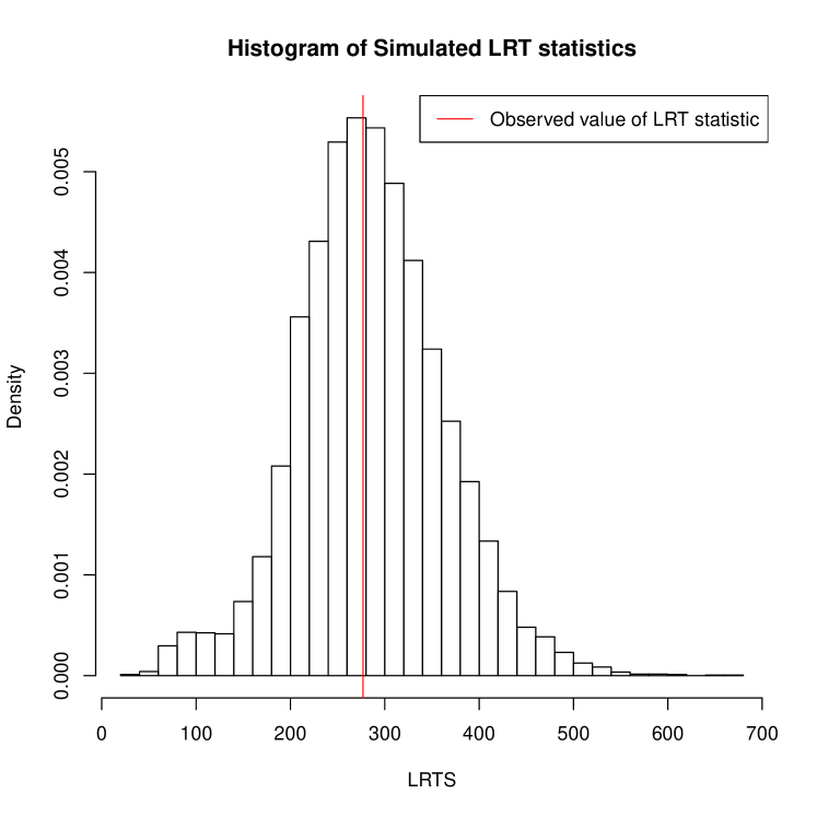
Figure 1: Histogram of LRT statistics obtained by simulating from the fitted one-component Markov chain from Frydman (2005). The approximate parametric bootstrap p-value is 0.528, suggesting the data is consistent with a single Markov chain as opposed to a mixture of two.

3.2 Selecting the number of mixture components using standard information criteria

Well-known model selection methods, particularly AIC, BIC and many other variants, all have the same general form: choose the model with the largest value of the difference

$$\Lambda_{k}-\pi_{k}\,,$$

where $\Lambda_{k}$ is the maximised log-likelihood over model $k$ and $\pi_{k}$ is a non-negative penalty which measures, in some sense, the “complexity” of model $k$.

Any such method is determined by the the pairwise differences $\pi_{\ell}-\pi_{k}$ for each $k\neq\ell$. For many methods, including AIC and BIC, this difference is a function of $d$, the “difference in number of free parameters” between the two models, alternatively the “number of parametric constraints” imposed on the larger model to give the smaller model. For AIC it is $2d$, for BIC it is $d\log n$, where $n$ is the sample size.

These methods suffer from an operational problem when trying to select the number of components in finite mixture models, because smaller models with fewer components are not uniquely identified within the larger models with more components. For example, consider a $k$-dimensional parametric family of densities $\{f(\cdot;\boldsymbol{\theta})\colon\boldsymbol{\theta}\in\mathbb{R}^{k}\}$ and define the two-component mixture model

$$g(\cdot;p,\boldsymbol{\theta})=(1-p)f(\cdot;\boldsymbol{\theta}_{0})+pf(\cdot;\boldsymbol{\theta})\,,$$

for some known reference value $\boldsymbol{\theta}_{0}$. Take as the smaller model the singleton $\{f(\cdot;\boldsymbol{\theta}_{0})$ and take as the larger model $\{g(\cdot;p,\boldsymbol{\theta})\colon 0\leq p\leq 1,\,\boldsymbol{\theta}\in\mathbb{R}^{k}\}$. The smaller model may be obtained from the larger model by imposing the $k$ constraints $\boldsymbol{\theta}=\boldsymbol{\theta}_{0}$, but it may also be obtained by imposing the single constraint $p=0$. Thus the value of $d$ here is ambiguous, so it is not clear how penalties for AIC and BIC are determined in this or similar cases.

We therefore caution against using information criteria of this form, which only depend on this value $d$, like AIC and BIC. More complicated methods are needed which take into account the non-standard behaviour of maximised likelihoods in these mixture models, for example AIC_mix introduced in Hui et al. (2015). A more detailed examination of this and similar methods is beyond the scope of the current paper, where the focus is on choosing between one and two components under the null hypothesis of one component. Once the limiting null distribution of the log-likelihood ratio statistic is determined, the limiting probability of selecting either model, using any form of complexity penalty when the null hyothesis is true can also be determined.

4 Exact asymptotics for detection of a two-state Markov chain mixture

We showed in the previous section that when fitting a mixture of two Markov chains (even if one of the states is absorbing) the LRT statistic for testing between one and two components tends to infinity in probability. Our simulation also showed that the rate of divergence is such that an observed statistic which seems highly significant when compared to a $\chi^{2}$ distribution may not be significant at all.

In this section we consider the simplest possible special case: where there are only two states, one of which is absorbing and all observations start in the non-absorbing state. Suppose that defaults occur with rate $\theta$. Then the time to default has an exponential distribution but if the observation window is limited to an interval $(0,T]$ there is a positive probability of defaulting after time $T$. Thus we may take each observation $X_{i}=\min(Y_{i},T)$ where $Y_{i}$ has exponential distribution with rate $\theta$ so that $X_{i}$ has a right-censored exponential distribution satisfying

$$P_{\theta}(X_{i}\leq x)=\begin{cases}0&\text{ for $x\leq 0$,}\\ 1-e^{-\theta x}&\text{ for $0<x<T$ and}\\ 1&\text{ for $x=T$.}\end{cases}$$

We may take as dominating measure the sum of Lebesgue measure on the interval $(0,T)$ and counting measure on $\{T\}$. The corresponding density is then given by

$$f(x;\theta)=\theta e^{-\theta x}1\left\{0<x<T\right\}+e^{-\theta T}1\left\{x=T\right\}\,.$$

Without loss of generality we assume that $X_{1},\ldots,X_{n}$ are independent with common density $f(\cdot;1)$. The statistic (2) becomes

$$\Lambda_{n}^{s}=\sup_{\begin{subarray}{c}0\leq p\leq 1\\ \theta>0\end{subarray}}\sum_{i=1}^{n}\log\left\{1+p\left[\frac{f(X_{i};\theta)}{f(X_{i};1)}-1\right]\right\}\,.$$ (15)

Theorem 2.

The statistic $\Lambda_{n}^{s}$ given by (15) satisfies

$$\Lambda_{n}^{s}=\log\log n+G_{n}-\log 4\pi\,,$$

where $G_{n}$ has an asymptotic Gumbel distribution, that is

$$P\{G_{n}\leq x\}\to e^{-e^{-x}}\,.$$ (16)

The method of proof closely follows that of the corresponding result in the one-sided, uncensored case, Liu et al. (2003, Theorem 2) whose steps we outline in subsection 4.1. In subsection 4.2, we describe the modifications required for proving the corresponding result in the two-sided censored case.

4.1 The one-sided, uncensored case of Liu et al. (2003).

Liu et al. (2003) derived the limiting null distribution of the statistic $\Lambda_{n}^{s}$ in the case of gamma scale mixtures (which includes uncensored exponential scale mixtures), but the test was one-sided in that the mean in the unknown second component was restricted to be smaller than the mean in the known, null component. We follow the same general approach for our censored case but with several notable differences, in particular that we are able to relax the one-sided restriction, mainly due to the censoring, as we shall see.

The main idea behind their method is to obtain a uniform version of the approximation (7) with careful control of the rate of the error term. The main tool used to achieve this is the approximation (on a suitable probability space) a version of the process $\{S_{n}(\theta)\}$ with a mean-zero Gaussian process $\{H_{n}(\theta)\}$ which has the property that the scale-transformed process $\left\{H_{n}\left(e^{s}+\frac{1}{2}\right)\right\}$ is stationary, satisfying

$$\rho(s,t)=E\left[H_{n}\left(e^{s}+\frac{1}{2}\right)H_{n}\left(e^{t}+\frac{1}{2}\right)\right]=2\left(e^{\frac{s-t}{2}}+e^{\frac{t-s}{2}}\right)^{-1}\,,$$

only depending on $(s,t)$ via $|s-t|$; moreover as $\Delta\to 0$,

$$\rho(t,t+\Delta)=1-\frac{\Delta^{2}}{8}+o\left(\Delta^{2}\right)\,,$$ (17)

while as $\Delta\to\infty$,

$$\rho(t,t+\Delta)\sim 2e^{-\frac{\Delta}{2}}\,.$$ (18)

The short-range condition (17) and long-range condition (18) mean that according to Leadbetter et al. (1983, Theorem 8.2.7), for any $L_{n}\to\infty$,

$$\sup_{0\leq s\leq L_{n}}H_{n}\left(e^{s}+\frac{1}{2}\right)=\sqrt{2\log L_{n}}+\frac{G_{n}-\log(4\pi)}{\sqrt{2\log L_{n}}}\,,$$ (19)

where $G_{n}$ denotes a generic random variable with an asymptotic Gumbel distribution, satisfying (16) above. By stationarity, the same applies to any interval of length $L_{n}$.

The remaining steps in their proof may be summarised as follows. Writing

$$I_{n}=\left(\log n,n(\log n)^{-4}\right)\,,$$

they show that

$$\sup_{\theta\in[1,\infty)\setminus I_{n}}S_{n}(\theta) =O_{p}\left\{(\log\log\log n)^{1/2}\right\}\,$$

and

$$\sup_{\theta\in I_{n}}\left|S_{n}(\theta)-H_{n}(\theta)\right| =O_{p}\left\{(\log n)^{-1}\right\}\,.$$

These two results together with (19) imply that with probability tending to 1,

$$M_{n} =\sup_{\theta\geq 1}S_{n}(\theta)=\sup_{\theta\in I_{n}}S_{n}(\theta)=\sup_{\theta\in I_{n}}H_{n}(\theta)+O_{p}\left\{(\log n)^{-1}\right\}\,.$$

This immediately yields

$$M_{n}=\sqrt{2\log\log n}+\frac{G_{n}-\log 4\pi}{\sqrt{2\log\log n}}\,,$$

where again $G_{n}$ satisfies (16), and the same is true replacing $M_{n}$ with $\sup_{\theta\in I_{n}}S_{n}(\theta)$.

The final steps involve showing that the profile likelihood $\Lambda_{n}^{p}(\theta)$ satisfies

$$\sup_{\theta\in[1,\infty)\setminus I_{n}}\Lambda_{n}^{p}(\theta) =O_{p}\left\{(\log\log\log n)^{1/2}\right\}$$

and

$$\sup_{\theta\in I_{n}}\Lambda_{n}^{p}(\theta) =\frac{1}{2}\left\{\sup_{\theta\in I_{n}}S_{n}(\theta)\right\}^{2}+o_{p}(1)\,.$$

These imply that

$$\Lambda_{n}^{s}=\sup_{\theta\geq 1}\Lambda_{n}^{p}(\theta)=\log\log n+G_{n}-\log 4\pi\,,$$

with $G_{n}$ satisfying (16).

4.2 The two-sided censored case

Liu et al. (2003) only considered $\theta\geq 1$ in their second mixture component because the same strategy cannot be applied for $0<\theta<1$; in particular for $0<\theta<\frac{1}{2}$ the score process has infinite variance and so the Gaussian process approximation fails. In short, the method fails if the second mixture component has a mean which is too large. However in our case, the censoring has the result of attenuating that problem and so it becomes possible to approximate the score process $\{S_{n}(\theta)\}$ with a Gaussian process $\{H_{n}(\theta)\}$ throughout the whole range $\theta>0$. The main modification required is to manage the fact that this Gaussian process is such that using the same change of scale,

$$\rho(t,t+\Delta) =E\left[H_{n}\left(e^{t}+\frac{1}{2}\right)H_{n}\left(e^{t+\Delta}+\frac{1}{2}\right)\right]$$

and

$$=\frac{2}{e^{\frac{\Delta}{2}}+e^{-\frac{\Delta}{2}}}\,\frac{1-e^{-T(e^{t}+e^{t+\Delta})}}{\sqrt{(1-e^{-2Te^{t}})(1-e^{-2Te^{t+\Delta}})}}$$

which is not free of $t$ as in the uncensored case. Thus the process $\left\{H_{n}\left(e^{t}+\frac{1}{2}\right)\right\}$ is not stationary. However, we show that it is locally stationary in the sense of Berman (1974) and Hüsler (1990), meaning that as $\Delta\to 0$,

$$\rho(t,t+\Delta)=1-V(t)\Delta^{2}+o\left(\Delta^{2}\right)\,,$$

for a continuous positive function $V(t)$ which is bounded away from zero and infinity and the $o\left(\Delta^{2}\right)$ term is uniform in $t$ (see Fitzpatrick, 2016, subsection 5.3.1 for details). Under an analogue of the long-range condition (18), namely

$$\sup_{t}\rho(t,t+\Delta)=o\left(\frac{1}{\log\Delta}\right)\,,$$

as $\Delta\to\infty$ (which is comfortably satisfied), a parallel theory of extremes for locally stationary Gaussian processes (see Hüsler, 1990, 1995) provides analogous limiting results.

The rest of the proof follows the same steps as for Liu et al. (2003, Theorem 2), with various technical modifications needed. We do not provide all the details here, but refer the reader to Fitzpatrick (2016, Chapter 5).

5 Concluding remarks

We have provided some general conditions which indicate when the standard $\chi^{2}$ approximation to the LRT statistic fails and may lead to false significance; our simulations in subsection 3.1 show that this discrepancy can be substantial. Our general advice is to always verify asymptotic approximations to p-values by simulation whenever possible. The precise limiting distribution we provide in section 4 for the case of two states indicates a very slow rate of divergence of $\log\log n$, however our simulation in section 3.1 shows that for a larger number of states the rate of divergence may be substantially faster. The rate is related to the complexity of the family of standardised score functions and both the dimensionality and effective range of maximisation (respectively 1 and $L_{n}\approx\log n$ in our example) of a corresponding approximating locally stationary Gaussian process. The dimensionality reflects the number of states while the effective range of maximisation reflects how the size of the convex hull of the sample is transformed under the appropriate local-stationarity-inducing transformation. Some indications of this are given in some elementary univariate exponential family mixture model examples in Stewart & Robinson (2003); see also Ingster (1997, 2001, 2002), Donoho & Jin (2004), Cai et al. (2011); Cai & Wu (2014); Hall & Stewart (2005) and Porter & Stewart (2020) for more on rates of convergence of the LRT statistic under both the null hypothesis and local alternatives in various two-component mixture models.

Appendix A R Code for parametric bootstrap

References

- Albert (1962) Albert, A. (1962). Estimating the infinitesimal generator of a continuous time, finite state Markov process. Ann. Math. Statist., 33, 727–753.
- Azaïs et al. (2006) Azaïs, J.-M., Gassiat, E., & Mercadier, C. (2006). Asymptotic distribution and local power of the log-likelihood ratio test for mixtures: bounded and unbounded cases. Bernoulli, 12, 775–799. URL: https://doi.org/10.3150/bj/1161614946. doi:10.3150/bj/1161614946.
- Azaïs et al. (2009) Azaïs, J.-M., Gassiat, E., & Mercadier, C. (2009). The likelihood ratio test for general mixture models with or without structural parameter. ESAIM Probab. Stat., 13, 301–327. URL: https://doi.org/10.1051/ps:2008010. doi:10.1051/ps:2008010.
- Berman (1974) Berman, S. M. (1974). Sojourns and extremes of Gaussian processes. Ann. Probability, 2, 999–1026.
- Bickel & Chernoff (1993) Bickel, P., & Chernoff, H. (1993). Asymptotic distribution of the likelihood ratio statistic in a prototypical non regular problem. In J. K. Ghosh, S. K. Mitra, K. R. Parthasararthy, & B. L. S. Prakasa Rao (Eds.), Statistics and Probability: A Raghu Raj Bahadur Festschrift (pp. 83–96). Wiley Eastern Limited.
- Cai et al. (2011) Cai, T. T., Jeng, X. J., & Jin, J. (2011). Optimal detection of heterogeneous and heteroscedastic mixtures. J. R. Stat. Soc. Ser. B Stat. Methodol., 73, 629–662.
- Cai & Wu (2014) Cai, T. T., & Wu, Y. (2014). Optimal detection of sparse mixtures against a given null distribution. IEEE Trans. Inform. Theory, 60, 2217–2232. URL: https://doi.org/10.1109/TIT.2014.2304295. doi:10.1109/TIT.2014.2304295.
- Chernoff (1954) Chernoff, H. (1954). On the distribution of the likelihood ratio. Annals of Mathematical Statistics, 25, 573–578.
- Cramér & Leadbetter (1967) Cramér, H., & Leadbetter, M. R. (1967). Stationary and related stochastic processes. Sample function properties and their applications. New York: John Wiley & Sons Inc.
- Dacunha-Castelle & Gassiat (1997) Dacunha-Castelle, D., & Gassiat, E. (1997). Testing in locally conic models, and application to mixture models. ESAIM: Probability and Statistics, 1, 285–317.
- Donoho & Jin (2004) Donoho, D., & Jin, J. (2004). Higher criticism for detecting sparse heterogeneous mixtures. Ann. Statist., 32, 962–994.
- Fitzpatrick (2016) Fitzpatrick, M. A. (2016). Multi-regime models involving Markov chains. Ph.D. thesis University of Sydney. URL: http://hdl.handle.net/2123/14530.
- Frydman (2005) Frydman, H. (2005). Estimation in the mixture of Markov chains moving with different speeds. J. Amer. Statist. Assoc., 100, 1046–1053. URL: http://dx.doi.org/10.1198/016214505000000024. doi:10.1198/016214505000000024.
- Fukumizu (2003) Fukumizu, K. (2003). Likelihood ratio of unidentifiable models and multilayer neural networks. Ann. Statist., 31, 833–851. URL: https://doi.org/10.1214/aos/1056562464. doi:10.1214/aos/1056562464.
- Garel (2001) Garel, B. (2001). Likelihood ratio test for univariate gaussian mixtures. Journal of Statistical Planning and Inference, 96, 325–350.
- Garel (2005) Garel, B. (2005). Asymptotic theory of the likelihood ratio test for the identification of a mixture. J. Statist. Plann. Inference, 131, 271–296. URL: https://doi.org/10.1016/j.jspi.2004.01.006. doi:10.1016/j.jspi.2004.01.006.
- Gassiat (2002) Gassiat, E. (2002). Likelihood ratio inequalities with applications to various mixtures. (pp. 897–906). volume 38. URL: https://doi.org/10.1016/S0246-0203(02)01125-1. doi:10.1016/S0246-0203(02)01125-1 en l’honneur de J. Bretagnolle, D. Dacunha-Castelle, I. Ibragimov.
- van de Geer (2000) van de Geer, S. A. (2000). Empirical Processes in M-estimation volume 6. Cambridge university press.
- Ghosh & Sen (1985) Ghosh, J. K., & Sen, P. K. (1985). On the asymptotic performance of the log likelihood ratio statistic for the mixture model and related results. In Proceedings of the Berkeley conference in honor of Jerzy Neyman and Jack Kiefer, Vol. II (Berkeley, Calif., 1983) Wadsworth Statist./Probab. Ser. (pp. 789–806). Wadsworth, Belmont, CA.
- Hall & Stewart (2005) Hall, P., & Stewart, M. (2005). Theoretical analysis of power in a two-component normal mixture model. J. Statist. Plann. Inference, 134, 158–179.
- Hartigan (1985) Hartigan, J. A. (1985). A failure of likelihood asymptotics for normal mixtures. In Proceedings of the Berkeley conference in honor of Jerzy Neyman and Jack Kiefer, Vol. II (Berkeley, Calif., 1983) Wadsworth Statist./Probab. Ser. (pp. 807–810). Wadsworth, Belmont, CA.
- Hui et al. (2015) Hui, F. K. C., Warton, D. I., & Foster, S. D. (2015). Order selection in finite mixture models: complete or observed likelihood information criteria? Biometrika, 102, 724–730. URL: https://doi.org/10.1093/biomet/asv027. doi:10.1093/biomet/asv027.
- Hüsler (1990) Hüsler, J. (1990). Extreme values and high boundary crossings of locally stationary Gaussian processes. Ann. Probab., 18, 1141–1158.
- Hüsler (1995) Hüsler, J. (1995). A note on extreme values of locally stationary Gaussian processes. J. Statist. Plann. Inference, 45, 203–213. Extreme value theory and applications (Villeneuve d’Ascq, 1992).
- Ingster (1997) Ingster, Y. I. (1997). Some problems of hypothesis testing leading to infinitely divisible distributions. Math. Methods Statist., 6, 47–69.
- Ingster (2001) Ingster, Y. I. (2001). Adaptive detection of a signal of growing dimension. I. Math. Methods Statist., 10, 395–421 (2002). Meeting on Mathematical Statistics (Marseille, 2000).
- Ingster (2002) Ingster, Y. I. (2002). Adaptive detection of a signal of growing dimension. II. Math. Methods Statist., 11, 37–68.
- Leadbetter et al. (1983) Leadbetter, M., Lindgren, G., & Rootzén, H. (1983). Extremes and Related Properties of Random Sequences and Processes. Springer-Verlag.
- Lehmann & Romano (2005) Lehmann, E. L., & Romano, J. P. (2005). Testing statistical hypotheses. Springer Texts in Statistics (3rd ed.). Springer, New York.
- Liu et al. (2003) Liu, X., Pasarica, C., & Shao, Y. (2003). Testing homogeneity in gamma mixture models. Scand. J. Statist., 30, 227–239.
- Liu & Shao (2003) Liu, X., & Shao, Y. (2003). Asymptotics for likelihood ratio tests under loss of identifiability. Annals of Statistics, 31.
- Liu & Shao (2004) Liu, X., & Shao, Y. (2004). Asymptotics for the likelihood ratio test in a two-component normal mixture model. J. Statist. Plann. Inference, 123, 61–81.
- Piterbarg (1996) Piterbarg, V. I. (1996). Asymptotic Methods in the Theory of Gaussian Processes and Fields. American Mathematical Society.
- Porter & Stewart (2020) Porter, T., & Stewart, M. (2020). Beyond hc: More sensitive tests for rare/weak alternatives. Ann. Statist., 48, 2230–2252. doi:10.1214/19-AOS1885.
- Stewart & Robinson (2003) Stewart, M., & Robinson, J. (2003). Extremes of normed empirical moment generating function processes. Extremes, 6, 319–333 (2005).
- van der Vaart & Wellner (1996) van der Vaart, A. W., & Wellner, J. A. (1996). Weak Convergence and Empirical Processes. Springer Series in Statistics. Springer.
- Yang (2005) Yang, Y. (2005). Can the strengths of AIC and BIC be shared? A conflict between model indentification and regression estimation. Biometrika, 92, 937–950. URL: http://biomet.oxfordjournals.org/content/92/4/937.abstract. doi:10.1093/biomet/92.4.937. arXiv:http://biomet.oxfordjournals.org/content/92/4/937.full.pdf+html.