Computing the solutions of the van der Pol equation to arbitrary precision

Abstract

We describe an extension of the Taylor method for the numerical solution of ODEs that uses Padé approximants to obtain extremely precise numerical results. The accuracy of the results is essentially limited only by the computer time and memory, provided that one works in arbitrary precision. In this method the stepsize is adjusted to achieve the desired accuracy (variable stepsize), while the order of the Taylor expansion can be either fixed or changed at each iteration (variable order).

As an application, we have calculated the periodic solutions (limit cycle) of the van der Pol equation with an unprecedented accuracy for a large set of couplings (well beyond the values currently found in the literature) and we have used these numerical results to validate the asymptotic behavior of the period, of the amplitude and of the Lyapunov exponent reported in the literature. We have also used the numerical results to infer the formulas for the asymptotic behavior of the fast component of the period and of the maximum velocity, which have never been calculated before.

1 Introduction

The Taylor method is one of the oldest methods for the numerical solution of ODEs: in fact the well–known Euler method is essentially a Taylor method of order one. Higher order Taylor methods have been explored in the literature, but their use is still not widespread. From our (partial) exploration of the literature, we have found refs. [1, 2, 3, 4, 5, 6, 7, 8] to be the most relevant to our discussion.

The paper by Deprit and Zahar [1] is possibly the first to show the advantages of using the Taylor method compared to a more standard Runge-Kutta-Nystrom algorithm: these authors found that the latter needs to use step size about $4000$ smaller to reach the same accuracy of the former. Corliss and Chang [2, 3] have applied the Taylor method to a series of problems (using fortran). The remaining papers, ref. [4] by Jorba and Zou and refs. [5, 6, 7, 8] by Barrio and collaborators, are particularly important because of their emphasis on achieving high precision. In general it is found that the high-order Taylor method is very competitive with other numerical methods when high accuracy is needed; moreover this method can be used to calculate the numerical solutions to certain class of ODEs with unprecedented accuracy (from the abstract of ref. [7]: "this methodology is the only one capable of reaching precision up to thousands of digits for ODEs").

At the same time, Jorba and Zou clearly state a limitation to the Taylor method: "The main drawback is that the Taylor method is an explicit method, so it has all the limitations of these kind of schemes. For instance, it is not suitable for stiff systems.". A discussion of the applicability of Taylor method for stiff ODEs is also contained in [5] .

The main goal of our paper is to describe an extension of the Taylor method that allows to obtain arbitrarily accurate numerical solutions even for stiff differential equations, such as the van der Pol equation that will be used in this paper as the ideal testing ground. The method that we propose is based on the use of Padé approximants rather than Taylor polynomials; we will show that the performance of the standard Taylor method is drastically improved both by enlarging the class of problems that can be attacked (e.g. stiff ODEs) and also by increasing the accuracy of the solutions with respect to the Taylor method with the same number of coefficients.

We will illustrate our method by applying it to the van der Pol oscillator, the most famous example of ODE supporting a limit cycle. For this problem there is an extensive literature, but surprisingly enough numerical solutions have never been calculated to a high level of accuracy, particularly for the stiff regime. Moreover the behavior of the period and amplitude of the limit cycle has been studied in depth both for small coupling (using perturbation theory, i.e. the Lindstedt-Poincaré method) and for large coupling (using asymptotic methods): by producing extremely accurate numerical solutions for a wide range of couplings we plan to show that it is possible to reproduce the known analytical results, but also to predict the asymptotic behavior of quantities not yet studied.

In our opinion, the quest for extremely precise numerical solutions is not a mere exercise of virtuosity but it has real applications: one cannot overstate the importance of predicting the behavior of a dynamical system while keeping under control the precision of the results. We believe that the technique described in this paper may be applied to a large number of problems for which accuracy is important.

The paper is organized as follows: in Section 2 we introduce our Padé – Taylor method (PTM) and discuss its main features; in Section 3 we consider the van der Pol oscillator and discuss the application of the Padé–Taylor method to it; in the subsections 3.1 and 3.2 we present the numerical results and apply appropriate extrapolation method to extract the leading asymptotic behavior for different quantities (particularly the period and the amplitude of the oscillator); finally, in Section 4 we draw our conclusions and discuss the possible directions of future work.

2 The Padé – Taylor method

Consider the ODE

$$\frac{d{\bf X}}{dt}=F(t,{\bf X}(t))\hskip 28.45274pt,\hskip 5.69046pt{\bf X}\in\mathbb{R}^{d}\hskip 5.69046pt,\hskip 5.69046ptt\in\mathbb{R}$$ (1)

with initial conditions

$${\bf X}(t_{0})={\bf X}_{0}$$ (2)

At $t>t_{0}$ the solution of eq. (1) can be approximated by a Taylor polynomial of order $N$

$${\bf X}(t)\approx{\bf X}(t_{0})+\left.\frac{d{\bf X}}{dt}\right|_{t_{0}}(t-t_{0})+\dots+\frac{1}{N!}\left.\frac{d^{N}{\bf X}}{dt^{N}}\right|_{t_{0}}(t-t_{0})^{N}$$ (3)

The Taylor coefficients in eq. (3) can be obtained by repeated derivations of eq. (1) and by subsequently setting $t=t_{0}$. Let $T_{0}$ be the radius of convergence of the power series obtained by taking the limit $N\rightarrow\infty$: clearly we are justified to use the polynomial (3) only for $t_{0}<t\ll t_{0}+T_{0}$. Without going to the extreme case where the power series is divergent ($T_{0}=0$), the reader may recognize that a finite value of $T_{0}$ sets an upper limit to the stepsize in the numerical integration of eq. (1). As a time step $\tau_{0}\ll T_{0}$ is chosen (in some way – we will discuss this point soon), a new approximation to the function at $t_{1}\equiv t_{0}+\tau_{0}$: from this approximate solution one can estimate the new Taylor coefficients corresponding to eq. (3) expanded arout $t_{1}$ and repeat the same arguments. In general we will have $\tau_{1}\neq\tau_{0}$ (variable stepsize): additionally, at each step one can use polynomials of different order if needed (variable order).

Of course we run into trouble if the power series becomes divergent (vanishing radius of convergence) at any finite time $t_{i}$: in this case $\tau_{i}=0$ is the only allowed stepsize.

The natural choice to extend the range of applicability of the power expansion is to substitute the Taylor expansion with a Padé approximant of appropriate order:

$$\mathcal{P}\left[{\bf X}(t)\right]_{[m,n]}=\frac{P_{m}(t-t_{0})}{Q_{n}(t-t_{0})}$$ (4)

where $P_{m}(t-t_{0})$ and $Q_{n}(t-t_{0})$ are polynomials of order $m$ and $n$ and the expansion of eq. (4) reproduces the first $N+1$ Taylor coefficients ($m+n=N$). Let $\tau_{i}^{(0)}$, with $i=1,\dots,n$, be the (complex) roots of the polynomial $Q_{n}(\tau)$: the smallest positive real root (if any) will limit the region of applicability of (4) to smaller values of the stepsize.

Let us now how come to the important question: how do we select a suitable stepsize $\tau_{0}$? The only limitations on $\tau_{0}$ that we have discussed so far are related to the radius of convergence of the power series at $t=t_{0}$ and to the possible presence of spurious singularities of the Padé approximant on the positive real axis. As a matter of fact one needs to select time-steps that are far enough from this spurious pole of the Padé approximant to avoid catastrophic loss of precision.

To determine the stepsize in a suitable way, we consider the residual

$$\mathcal{R}[\tilde{\bf X}]\equiv\left|\frac{d{\bf\tilde{\bf X}}}{dt}-F(t,{\bf\tilde{X}}(t))\right|\geq 0$$ (5)

obtained by substituting the approximate solution $\tilde{\bf X}(t)\equiv\mathcal{P}\left[{\bf X}(t)\right]_{[m,n]}$ inside eq. (1). Since the residual vanishes at $t=t_{0}$, $\mathcal{R}[\tilde{\bf X}]_{t=t_{0}}=0$, we expect it to grow in size at later times $t>t_{0}$, unless $\tilde{\bf X}$ is a solution of eq. (1) (in this case it vanishes identically). In other words, the residual grows monotonically in a sufficiently small region to the right of $t_{0}$ and we can constrain the loss of precision of the numerical solution for $t_{0}<t<t_{0}+\tau_{0}$, by choosing $\tau_{0}$ in a suitable way.

This is done by introducing a real parameter $\delta$, with $0<\delta\ll 1$, such that $\mathcal{R}[\tilde{\bf X}]\leq\delta$ for $t_{0}\leq t\leq t_{0}+dt_{0}$ . The value of the time step $dt_{0}$ found in this way ensures that the error made in approximating the exact solution with ${\bf\tilde{X}}$ is bounded at all times $t_{0}\leq t\leq t_{0}+dt_{0}$.

The process can now be iterated: moving at the time $t_{1}=t_{0}+dt_{0}$ we can repeat the previous steps by considering eq. (1) with initial conditions ${\bf X}(t_{1})={\bf\tilde{X}}(t_{1})$ and find a new time step and consequently new initial conditions at a time $t_{2}=t_{1}+dt_{1}$.

At each stepsize there is the freedom of changing the order of the Padé approximant used in the calculation, so that we can regard our method as a variable stepsize variable order Padé-Taylor (VSVO-PT) method.

In the next section we illustrate the method by applying it to the van der Pol equation.

3 The van der Pol oscillator

The van der Pol equation [9]

$$\ddot{x}(t)+x(t)=\mu\dot{x}(t)\left(1-x^{2}(t)\right)\hskip 28.45274pt,\hskip 28.45274pt\mu\geq 0$$ (6)

is an example of nonlinear ordinary differential equation that supports a limit cycle: for $\mu>0$, regardless of the initial conditions (with the exclusion of $x(0)=\dot{x}(0)=0$), the system evolves in time towards a limit cycle with fixed period and amplitude (both functions of the parameter $\mu$). The trajectory that the solution describes in phase space spirals in or out (depending on the initial conditions) towards a close orbit that for $0<\mu\ll 1$ closely resembles that of a harmonic oscillator while for $\mu\gg 1$ results in a highly deformed loop (reflecting the presence of two very different – slow and fast – regimes).

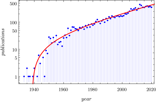
Figure 1: Publications per year found with a search of the keyword "van der Pol equation" in google scholar. The solid line is the fit $N(t)=-28.17+6.31\times e^{0.034t-64.66}$.

The van der Pol equation constitutes the perfect testing ground for our method, because it represents a challenging problem, which has attracted (and continues to attract) much interest in the literature. This interest is reflected in Fig. 1 where we report the number of publications per year found in google scholar under the keyword "van der Pol equation". The recent paper by Ginoux and Letellier provides an historical account on the origins of the van der Pol equation [10].

Following [11] we classify the strategies for studying the limit cycle of the vdP equation into three categories:

• numerical studies [12, 13, 14, 15, 16, 17], where the eq. (6) is solved numerically for some finite value of $\mu$ (apparently the largest value of $\mu$ for which the period and amplitude have been calculated is $\mu=200$ in ref. [14]); the accuracy of the results progressively worsens as $\mu$ gets larger ;

• asymptotic studies [23, 24, 25, 26, 27, 28, 29, 14, 30, 31, 32], where the behavior of the solution (particularly the period and the amplitude of the limit cycle) is established for $\mu\rightarrow\infty$; it is remarkable that as early as in 1944 Haag [25] and then in 1947 Dorodnitsyn [26] were able to approximate the asymptotic behavior of the period and the amplitude of the limit cycle of the van der Pol oscillator. For a discussion of the work of Dorodnitsyn, see ref. [33], written to celebrate the centenary of the birth of A.A. Dorodnitsyn.

• perturbative studies [35, 36, 37, 38, 39, 40, 41, 42, 11], where the behavior of the solution is established for $\mu\rightarrow 0$ (the perturbative series is a power series in $\mu$ with finite radius of convergence);

In the first category we find the works of Krogdahl [12], Urabe [13], Zonnenfeld [15], Clenshaw [16] and Greenspan [17] (all published between 1960 and 1972!). Note that the second method used by Greenspan in [17] to solve numerically eq. (6) is a Taylor method of order $8$.

Later works on the van der Pol oscillator are mainly interested in the study of the perturbation series for the solution, which is most efficiently obtained by applying the Lindstedt-Poincaré method. The numerical results of refs. [12, 13, 15, 16, 17] are used in those works to validate the accuracy of the resummation schemes adopted (see for instance Table 4 of [38], Table 2 of [39] and Table 2 of [40]). Strictly speaking, the use of the perturbation series for the period (amplitude) of the oscillator is limited to the region $\mu\leq\mu_{T}$ ($\mu\leq\mu_{A}$), where $\mu_{T}$ is the radius of convergence of the series . For $\mu>\mu_{T,A}$, different techniques can be applied to improve the convergence of the series, with some success (see [38, 40, 11]). In this regime however the numerical results are far more precise than the results based on perturbation theory, which can explain only in part the lack of interest in deriving far more precise numerical results. In our view another reason for the scarcity of numerical results is the difficulty in obtaining accurate numerical solutions of eq. (6) in the stiff regime ($\mu\gg 1$).

We will now apply to the van der Pol equation the procedures explained in the previous section for the general case.

We start at $t=t_{0}$, where the initial conditions $x(t_{0})=x_{0}$ and $\dot{x}(t_{0})=x^{\prime}_{0}$ are provided and consider the power series solution

$$x(t)=\sum_{k=0}^{\infty}c_{k}(t-t_{0})^{k}$$ (7)

with $c_{0}=x(t_{0})$ and $c_{1}=\dot{x}(t_{0})$. The coefficients $c_{k}$ with $k\geq 2$ can be obtained in terms of the nonlinear recurrence relation

$$\begin{split}c_{k+2}&=\frac{-c_{k}+\mu(k+1)c_{k+1}-\mu\sum_{k_{1}=1}^{k+1}\sum_{k_{2}=0}^{k-k_{1}+1}k_{1}\ c_{k_{1}}\ c_{k_{2}}\ c_{k-k_{1}-k_{2}+1}}{(k+1)(k+2)}\end{split}$$ (8)

This equation allows one to calculate exactly a large number of coefficients of the power series and thus estimate its radius of convergence. In Fig. 2 we estimate the radius of convergence of the power series (7) for $\mu=100$, $x_{0}=2$ and $x^{\prime}_{0}=0$, which turns out to be $\approx 1/26$.

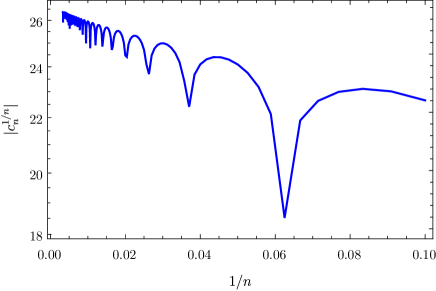
Figure 2: Approximate radius of convergence of the power series obtained from eq. (8), for $\mu=100$, $x_{0}=2$ and $x^{\prime}_{0}=0$. We plot $1/R\approx|c_{n}^{1/n}|$ as a function of the order $n$ of the Taylor coefficient (root test). A similar estimate can be obtained using the Padé approximants.

In Fig. 3 we plot the real poles of the Padé approximant of order $[n,n]$ for $\mu=100$, $x_{0}=2$ and $x^{\prime}_{0}=0$: we see that Padé of order $3$,$5$,$7$ and $9$ have a positive real root. For example for $n=3$ the root is approximately $\tau\approx 0.03091366759$, which constitutes an upper limit to the stepsize. Similar behaviors are also observed for smaller values of $\mu$, but in that case the real positive roots are much larger (thus allowing to span a much greater interval of time).

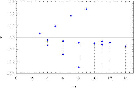
Figure 3: Real poles of the Padé approximant of order $[n,n]$ for $\mu=100$, $x_{0}=2$ and $x^{\prime}_{0}=0$. Multiple real roots of the same order are joined by a dashed line.

In Fig. 4 we plot the residual for $\mu=100$, $x_{0}=2$ and $x^{\prime}_{0}=0$, again using only the first $13$ coefficients: the residual obtained using a diagonal Padé approximant is about $10^{6}$ smaller than the corresponding residual built on the Taylor polynomial with the same number of coefficients. To get an idea, in this case the region for which $\mathcal{R}<10^{-30}$ is about $3$ times larger when the Padé approximants are used.

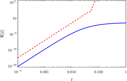
Figure 4: Residual obtained using the first $13$ Taylor coefficients for $\mu=100$, $x_{0}=2$ and $x^{\prime}_{0}=0$. The solid line is the result obtained using diagonal Padé approximants while the dashed line uses the polynomial of order $12$.

There is an important advantage in using our method (or the Taylor method) for the calculation of the period and amplitude of the limit cycle (or more in general of any periodic solution): although these methods work by performing discrete time steps, $t_{0}\rightarrow t_{1}\rightarrow t_{2}\rightarrow\dots$, the solution is also known at any arbitrary time between any two consecutive times steps, in terms of a Padé approximant (in our case) or of a Taylor polynomial (for the Taylor method). In our method, when moving from time $t_{i}$ to time $t_{i+1}$, we expect that the maximum error occurs at $t=t_{i+1}$, where the residual takes the maximum value $\delta$. In this way we can estimate within the same accuracy both the location of a maximum or a minimum and the value of the solution at this point.

The situation is be completely different using the Runge-Kutta method: for example, Odani [43] has estimated the amplitude of the van der Pol oscillator for a limited set of values of the coupling using the Runge-Kutta method with a stepsize of $2^{-20}$! Even so the results reported by Odani contain only $5$ decimals. Notice that refs. [43, 44, 45, 46, 47] deal with the problem of determining the maximum amplitude of the limit cycle.

In our case the procedure to estimate the period and the amplitude of the oscillator is straightforward: we pick the initial conditions (typically we choose $x_{0}=2$ and $x^{\prime}_{0}=0$) and iterate our method until a change in the sign of the velocity is detected; at this point we know that a minimum of the solution can be found between the two last time steps and we can look for the zero of the derivative of the Padé approximant contained in this region. The value of the solution at this point (changed of sign) is then used as the new $x_{0}$ in the initial conditions (we set the time to zero at this point) and the whole procedure is repeated. The time elapsed from $t=0$ to the instant where the derivative changes sign is essentially the half–period. This process is iterated until the amplitude and the period have converged to a sufficiently large number of digits (alternatively the same process can be carried out by looking for two changes of sign in the derivative, which in turn would provide directly the period).

Importantly, we have the nice bonus that the number of iterations that are needed to reach the desired level of accuracy is much smaller in the stiff regime, where the transient behavior of the solution decays more rapidly with time (the number of time steps however increases, both because of the larger period, which grows with $\mu$, and because of the need for smaller steps in the regions where the derivative is large).

The accuracy that we can hope to reach for the period and the amplitude is essentially determined by $\delta$ (provided that the number of digits used in the calculation is sufficiently large): in this way, one can expect to improve the numerical estimates by using a sufficiently small $\delta$ and working with large enough digits. In the next section we provide an independent check of this claim can be done by comparing the purely numerical results with the analytical results both for $\mu\ll 1$ (perturbative) and for $\mu\gg 1$ (asymptotic – stiff).

3.1 Numerical results

We have obtained numerical results for the period and the amplitude of the limit cycle of the vdP oscillator for a series of values of $\mu$, starting at $\mu=1$ and going up to $\mu=500$ (well beyond the range of values studied in the literature). In the tables 1 and 2 we report the period and the amplitude of the limit cycle, obtained by working with the Padé-Taylor method, for $\mu=100$ (stiff), with different values of $\delta$. From these tables we see that the results appear to converge quite fast (we expect that the best results in the table, corresponding to $\delta=10^{-100}$, have more than $100$ digits correct).

In separate tables we have reported the values of the period (tables 3, 4, 5), of the amplitude (tables 6, 7, 8), of the maximum velocity (tables 9, 10,11), of the fast component of the period  (tables 12, 13, 14) and of $-\lambda_{2}/\mu$, $\lambda_{2}$ being the Lyapunov exponent (tables 15, 16, 17) .

Although Tables 1 and 2 provide an indication of the accuracy of our results, it is possible to perform an independent check by comparing these numerical results with the perturbative results obtained with the Lindstedt-Poincaré method (in ref. [11] we have worked out analytically the LP to order $308$ and numerically to order $859$ – in this case the coefficients are calculated with $1000$ digits).

This comparison can be done directly only for $\mu<\mu_{T,A}\approx 1.85$ (radius of convergence of the perturbative series): for $\mu=1$ the sum of the first $308$ terms of the LP series for the period and the amplitude are in excellent agreement with the numerical results obtained with the PTm:

$$T^{({\rm num})}-T^{(LP)}\approx 3.57\times 10^{-87}$$ (9)

and

$$A^{({\rm num})}-A^{(LP)}\approx 1.97\times 10^{-87}$$ (10)

The perturbative results, however, can be extended beyond the radius of convergence of the series, by using a Padé approximant (we opted for a diagonal Padé $[150,150]$). For $\mu=1$, the agreement between the Padé approximant and the numerical results is now extended to more than $100$ decimals:

$$T^{({\rm num})}-T^{(LP-Pade)}\approx-8.2\times 10^{-104}$$ (11)

and

$$A^{({\rm num})}-A^{(LP-Pade)}\approx-5.17\times 10^{-107}$$ (12)

Even for $\mu>\mu_{T,A}$, where the LP series does not converge, there is a remarkable agreement between the numerical results and those obtained using the Padé approximants, for $\mu\leq 10$.

This comparison is performed in Fig. 5, where we appreciate that, for $\mu\leq 4$, the results agree to more than $20$ decimals. This observation justifies using the Padé approximant for the amplitude to estimate quite precisely the maximum amplitude of limit cycle of the van der Pol equation, that has been studied in a series of papers, ref. [43, 44, 45, 46, 47], but never calculated with high precision. In Fig. 6 we plot the Padé approximant for the amplitude (solid line) and compare it with the upper bound conjectured by Odani  [43]. Our estimated value for the maximum amplitude is $A^{(max)}=2.0234222556061133094$ for $\mu=3.2940126635728034197$ (which complies with Odani’s conjectured upper bound $2.0235$).

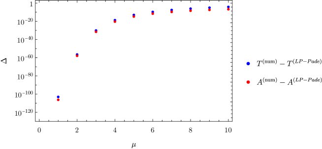
Figure 5: $\Delta_{T}=|T^{({\rm num})}-T^{(LP-Pade)}|$ and $\Delta_{A}=|A^{({\rm num})}-A^{(LP-Pade)}|$ as functions of $\mu$. Diagonal Padé approximants of order $[150,150]$ are used.

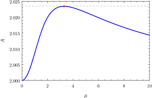
Figure 6: Amplitude of the limit cycle of the van der Pol oscillator obtained from the Padé approximant of order $[150,150]$ of the perturbative (LP) expansion. The horizontal dashed line corresponds to the upper bound conjectured by Odani [43], $A^{\rm(Odani)}=2.0235$. The red dot is the maximum value taken by the Padé approximant, $A^{(max)}=2.0234222556061133094$ for $\mu=3.2940126635728034197$.

In Fig. 7 we compare the stepsize of the PTm (normalized to the period) for different values of $\mu$; observe that the number of steps required to cover the whole period appears to scale as $\propto\mu^{5/3}$ (see Fig. 8). The corresponding solutions are displayed in Fig. 9.

Figure 7: Stepsize of the Padé-Taylor method with $\delta=10^{-100}$, using $201$ coefficients, for $\mu=1,10,100,500$.

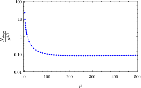
Figure 8: Number of steps used by the Padé-Taylor method with $\delta=10^{-100}$, and $201$ coefficients, as function of $\mu$.

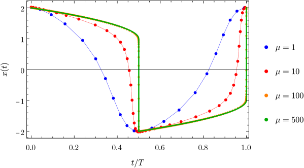
Figure 9: Solutions to the vdP equation for $\mu=1,10,100,500$ using the Padé-Taylor method with $\delta=10^{-100}$, and $201$ coefficients.

The reader may be skeptical on the necessity of calculating the period, the amplitude and more in general the limit cycle with such large precision as we claim having reached, but we hope that our next application will convince the most critical reader.

3.2 Extrapolation

In this section we adapt the discussion of Ref. [48], where the Richardson extrapolation was applied to the finite difference calculation of the Laplacian eigenvalues on complicated non-tensor domains in two dimensions.

In the previous section we have obtained very precise numerical results for different quantities (period, amplitude, maximum velocity, Lyapunov exponent, etc) related to the limit cycle of the van der Pol equation for different values of $\mu$. Let $\mathcal{O}$ be such quantity and consider a sequence of values $\mathcal{O}_{1}$, $\mathcal{O}_{2}$, …, corresponding to different values of the parameter, $\mu_{1}$, $\mu_{2}$, ….

For $\mu\gg 1$, the behavior of $\mathcal{O}(\mu)$ may be approximated as

$$\mathcal{O}(\mu)\approx\sum_{k=0}^{\infty}c_{k}f_{k}(\mu)=c_{0}f_{0}(\mu)+c_{1}f_{1}(\mu)+\dots$$ (13)

where $f_{0}(\mu)\gg f_{1}(\mu)\gg f_{2}(\mu)\gg\dots$, for $\mu\rightarrow\infty$. For the case $\mathcal{O}(\mu)=T(\mu)$, for example, several terms of the asymptotic formula has been derived in [23, 24, 25, 26, 27, 28, 29] and correspond to choosing

$$\begin{split}f_{0}(\mu)&=\mu\\ f_{1}(\mu)&=\mu^{-1/3}\\ f_{2}(\mu)&=\frac{\log\mu}{\mu}\\ f_{3}(\mu)&=\frac{1}{\mu}\end{split}$$ (14)

If we dispose of $N$ values of $\mathcal{O}$, for different values of $\mu$, and restrict our calculation to the first $N$ functions $f_{i}(\mu)$, we can write the system of equations

$$\begin{split}\mathcal{O}_{1}&=c_{0}f_{0}(\mu_{1})+c_{1}f_{1}(\mu_{1})+\dots+c_{N-1}f_{N-1}(\mu_{1})\\ \mathcal{O}_{2}&=c_{0}f_{0}(\mu_{2})+c_{1}f_{1}(\mu_{2})+\dots+c_{N-1}f_{N-1}(\mu_{2})\\ &\dots\\ \mathcal{O}_{N}&=c_{0}f_{0}(\mu_{N})+c_{1}f_{1}(\mu_{N})+\dots+c_{N-1}f_{N-1}(\mu_{N})\\ \end{split}$$ (15)

which can be cast in matrix form as

$$\mathbf{R}\left(\begin{array}[]{c}c_{0}\\ c_{1}\\ \dots\\ c_{N-1}\\ \end{array}\right)=\left(\begin{array}[]{c}\mathcal{O}_{1}\\ \mathcal{O}_{2}\\ \dots\\ \mathcal{O}_{N-1}\\ \end{array}\right)$$ (16)

where

$$\mathbf{R}\equiv\left(\begin{array}[]{cccc}f_{0}(\mu_{1})&f_{1}(\mu_{1})&\dots&f_{N-1}(\mu_{1})\\ f_{0}(\mu_{2})&f_{1}(\mu_{2})&\dots&f_{N-1}(\mu_{2})\\ \dots&\dots&\dots&\dots\\ f_{0}(\mu_{N})&f_{1}(\mu_{N})&\dots&f_{N-1}(\mu_{N})\\ \end{array}\right)$$ (17)

The solution to eq. (15) can be obtained either by using the inverse matrix $\mathbf{R}^{-1}$

$$\left(\begin{array}[]{c}c_{0}\\ c_{1}\\ \dots\\ c_{N-1}\\ \end{array}\right)=\mathbf{R}^{-1}\left(\begin{array}[]{c}\mathcal{O}_{1}\\ \mathcal{O}_{2}\\ \dots\\ \mathcal{O}_{N-1}\\ \end{array}\right)$$ (18)

or by using Cramer’s rule.

A further improvement can be obtained by performing a Richardson-Padé extrapolation, as done in ref. [48]; in this case we assume

$$\mathcal{O}(\mu)\approx\frac{\sum_{k=0}^{N}c_{k}f_{k}(\mu)}{1+\sum_{k=1}^{M}d_{k}g_{k}(\mu)}$$ (19)

where $\lim_{\mu\rightarrow\infty}g_{k}(\mu)=0$ (a convenient choice is $g_{k}(\mu)=\frac{1}{\mu^{k}}$, $k=1,2,\dots$). By using a rational extrapolation, we may be able to describe more precisely also the behavior of the observable for smaller values of $\mu$.

Using $N+M+1$ numerical results one can write the system of equations

$$\begin{split}\mathcal{O}_{1}&=c_{0}f_{0}(\mu_{1})+c_{1}f_{1}(\mu_{1})+\dots+c_{N-1}f_{N-1}(\mu_{1})\\ &-\left[d_{1}g_{1}(\mu_{1})+\dots+d_{M}g_{M}(\mu_{1})\right]\mathcal{O}_{1}\\ \mathcal{O}_{2}&=c_{0}f_{0}(\mu_{2})+c_{1}f_{1}(\mu_{2})+\dots+c_{N-1}f_{N-1}(\mu_{2})\\ &-\left[d_{1}g_{1}(\mu_{2})+\dots+d_{M}g_{M}(\mu_{2})\right]\mathcal{O}_{1}\\ &\dots\\ \mathcal{O}_{N+M+1}&=c_{0}f_{0}(\mu_{N+M+1})+\dots+c_{N-1}f_{N-1}(\mu_{N+M+1})\\ &-\left[d_{1}g_{1}(\mu_{N+M+1})+\dots+d_{M}g_{M}(\mu_{N+M+1})\right]\mathcal{O}_{1}\\ \end{split}$$ (20)

which can be cast in matrix form as

$$\tilde{\mathbf{R}}\left(\begin{array}[]{c}c_{0}\\ \dots\\ c_{N}\\ d_{1}\\ \dots\\ d_{M}\\ \end{array}\right)=\left(\begin{array}[]{c}\mathcal{O}_{1}\\ \mathcal{O}_{2}\\ \dots\\ \mathcal{O}_{N+M+1}\\ \end{array}\right)$$ (21)

where

$$\begin{split}\tilde{\mathbf{R}}\equiv\left(\begin{array}[]{cccccc}f_{0}(\mu_{1})&\dots&f_{N-}(\mu_{1})&-g_{1}(\mu_{1})\mathcal{O}_{1}&\dots&-g_{M}(\mu_{1})\mathcal{O}_{1}\\ f_{0}(\mu_{2})&\dots&f_{N-}(\mu_{2})&-g_{1}(\mu_{2})\mathcal{O}_{1}&\dots&-g_{M}(\mu_{2})\mathcal{O}_{2}\\ \dots&\dots&\dots&\dots&\dots&\dots\\ f_{0}(\mu_{N+M+1})&\dots&f_{N-}(\mu_{N+M+1})&-g_{1}(\mu_{N+M+1})\mathcal{O}_{N+M+1}&\dots&-g_{M}(\mu_{N+M+1})\mathcal{O}_{N+M+1}\\ \end{array}\right)\end{split}$$ (22)

Once again we can solve these equations either by using the inverse of $\tilde{\mathbf{R}}$ or by applying Cramer’s rule.

Of course the implementation of the Richardson and Richardson-Padé extrapolation requires to identify as many $f_{i}(\mu)$ as possible, which may be a difficult task in general. Some of these functions may be provided by previous asymptotic calculations, as for the case of the period and the amplitude of the limit cycle, but the remaining functions need to be "guessed". In an empirical approach one may select functions that lead to a faster convergence of the extrapolated results and discard functions whose coefficients are abnormally small.

Determining these functions rigorously is most likely a very difficult task: for the case of the Dirichlet eigenvalues of the Laplacian on a L-shaped membrane, for which the first correction to the lowest eigenvalue has been proved to behave as $h^{4/3}$ ($h$ is the grid spacing), the next few non-integer exponents have not been derived rigorously and, quoting Kuttler and Sigillito [51], “the exact form of the first several terms in the asymptotic formula for specific regions where no boundary interpolation is required is a nice problem at about the level of a doctoral thesis”. The fact that this problem is still open can be taken as an indication of its difficulty.

The extrapolation carried out in [48], where we tried to guess these exponents, resulted in obtaining very precisely the lowest eigenvalues of the L-shaped membrane (later confimed by the results obtained in ref. [52] using a different method) and the most precise estimate to date of the lowest eigenvalues of the pair of isospectral domains of ref. [53] (see also Refs. [49, 50] for further example of applications of the Richardson and Richardson-Padé extrapolations).

In Tables 12, 13 and 14 we report the precise numerical values of the times $T_{\rm fast}$ for different values of $\mu$.

We perform a Richardson extrapolation using the functions

$$\begin{split}f_{0}(\mu)=\frac{\log\mu}{\mu}\hskip 8.5359pt,\hskip 8.5359ptf_{1}(\mu)&=\frac{1}{\mu}\hskip 8.5359pt,\hskip 8.5359ptf_{2}(\mu)=\frac{1}{\mu^{2}}\hskip 28.45274pt\dots\\ \end{split}$$ (23)

and use the last $50$ numerical values to estimate the leading behavior of $T_{\rm fast}(\mu)$ for $\mu\gg 1$.

Our analysis shows that

$$T_{\rm fast}(\mu)\approx 1.33333333333333333334\ \frac{\log\mu}{\mu}+\frac{3.5305579106695527878}{\mu}+\dots$$ (24)

where one can observe that $1.33333333333333333334-4/3\approx 6.6\times 10^{-21}$ and $3.5305579106695527878-\left(\frac{4}{3}+\log 9\right)\approx 7.2\times 10^{-17}$.

We then have

$$T_{\rm fast}(\mu)\approx\frac{4}{3}\ \frac{\log\mu}{\mu}+\left(\frac{4}{3}+\log 9\right)\frac{1}{\mu}+\dots$$ (25)

The slow component of the period, $T_{\rm slow}$ is obtained from the condition $T_{\rm slow}=T-T_{\rm fast}$. In this case the Richardson extrapolation provides

$$\begin{split}T_{\rm slow}(\mu)&\approx 1.6137056388801093811656\ \mu+\frac{7.0143222313792851710947}{\mu^{1/3}}\\ &-1.99999999955\frac{\log(\mu)}{\mu}-\frac{4.853823019}{\mu}+\dots\end{split}$$ (26)

The accuracy of the first $3$ numerical coefficients allows to guess their exact values

$$\begin{split}T_{\rm slow}(\mu)\approx(3-\log 4)\mu-\frac{3\alpha}{\mu^{1/3}}-2\frac{\log\mu}{\mu}-\frac{4.853823019}{\mu}+\dots{}\end{split}$$ (27)

where $\alpha$ is the first zero of the Airy function ${\rm Ai}(x)$.

We can improve the estimate of the last coefficient by performing the Richardson extrapolation on the data where the contributions of the three first terms is taken out: in this case we obtain the slightly better value $-4.85382301173$.

By combining the formulas for the fast and slow periods, we obtain the asymptotic formula for the period of the vdP oscillator in the form

$$\begin{split}T(\mu)\approx(3-\log 4)\mu-\frac{3\alpha}{\mu^{1/3}}-\frac{2}{3}\frac{\log\mu}{\mu}-\frac{1.323265101}{\mu}+\dots{}\end{split}$$ (28)

which coincides with eq. (4) of Ref. [14], apart from last term that reads $-\frac{1.3246}{\mu}$. The coefficient $-1.3246$ used by Ponzo and Wax had been estimated earlier by Urabe [13].

It is interesting to observe that the formulas for the period given by Dorodnitcyn [26, 27] and Urabe [13] contain a different coefficient for the term $\log\mu/\mu$, $-22/9$ and $-1/3$ respectively. Ponzo and Wax were able to establish what is now accepted as the correct coefficient $-2/3$ by performing a numerical calculation up to $\mu=200$ (see Table 1 of ref. [14]).

By performing a Richardson-Padé extrapolation we are able to describe the numerical values for the amplitude in an excellent way, up to $\mu\approx 2$ (see Fig. 10). In fact the Richardson-Padé extrapolation is so accurate that it reproduces the first $10$ decimals of the value of the maximum amplitude obtained using the Padé approximant of order $[150,150]$ for the Lindstedt-Poincaré expansion! Similarly the value of $\mu$ corresponding to this maximum agrees within $8$ decimals with the value previously obtained.

While the expression for the amplitude obtained with Richardson-Padé is too lengthy to be reported here, it is useful to approximate it for $\mu\gg 1$, where it reads:

$$\begin{split}A&\approx 2.000000000000000000000084+\frac{0.77936913681989}{\mu^{4/3}}\\ &-\frac{0.5925925919\log(\mu)}{\mu^{2}}-\frac{0.8761741716}{\mu^{2}}\\ &-\frac{0.1988699974}{\mu^{8/3}}+\frac{0.1914226901}{\mu^{3}}-\frac{0.01149412656\log(\mu)}{\mu^{3}}+\dots\end{split}$$ (29)

It is easy to guess the exact form for the first three coefficients and obtain

$$\begin{split}A&\approx 2-\frac{\alpha}{3\mu^{4/3}}-\frac{27}{16}\frac{\log\mu}{\mu^{2}}-\frac{0.8761741716}{\mu^{2}}\\ &-\frac{0.1988699974}{\mu^{8/3}}+\frac{0.1914226901}{\mu^{3}}-\frac{0.01149412656\log(\mu)}{\mu^{3}}+\dots\end{split}$$ (30)

which agrees with the asymptotic formula for the amplitude, while adding few extra terms.

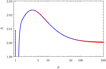
Figure 10: Richardson-Padé extrapolation for the amplitude of the limit cycle of the vdP oscillator (solid line). The dots are the numerical values for the amplitude reported in Tables 6, 7 and 8.

In the case of the maximum of $\dot{x}$ (corresponding to the numerical results in Tables 9, 10 and 11) using Richardson extrapolation we have found, on purely numerical grounds, the behavior

$$\max\left\{\dot{x}\right\}\approx\frac{4}{3}\mu-\frac{\alpha}{\mu^{1/3}}+\frac{4}{9}\frac{\log\mu}{\mu}+\dots$$ (31)

This formula has not been obtained before.

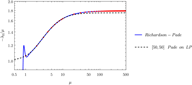
Figure 11: $-\lambda_{2}/\mu$ as a function of $\mu$ ($\lambda_{2}$ is the Lyapunov exponent). The dots are the precise numerical results obtained with the TPm; the solid blue line is the Richardson-Padé extrapolation of the numerical results, whereas the dashed line is the $[50,50]$ Padé approximant of the Lindstedt-Poincaré series.

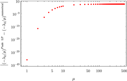
Figure 12: $\left|(-\lambda_{2}/\mu)^{Pade\ {\rm LP}}-(-\lambda_{2}/\mu)^{{\rm numerical}}\right|$ as a function of $\mu$.

Finally we consider the Lyapunov exponent, for which the asymptotic behavior has been established in ref. [34]. By performing the Richardson-Padé extrapolation of the numerical results, we have found that, for $\mu\gg 1$, the quantity $-\lambda_{2}/\mu$ behaves approximately as

$$\begin{split}-\lambda_{2}/\mu&\approx 1.7886126760534475020333538-3.427876368721168125\mu^{-4/3}\\ &-0.913585588576346183705582275127144801985703792607697195\frac{\log(\mu)}{\mu^{2}}\\ &-\frac{1.016871272807540550530978993562345482080521280}{\mu^{2}}+\dots\end{split}$$ (32)

The coefficient of the term $\mu^{0}$ agrees to $24$ digits with the predicted coefficient of [34], $\frac{3+\log(16)}{6-\log(16)}$; the coefficient of the term $\mu^{-4/3}$ agrees to $15$ digits with the predicted coefficient of [34], $-\frac{3(\log(256)-3)\alpha}{2(\log(4)-3)^{2}}$.

Alternatively one can obtain a perturbative expression for $-\lambda_{2}/\mu$ using the Lindstedt-Poincaré method; using the results previous obtained in [11] we can write the first few terms read 

$$\left.-\frac{\lambda_{2}}{\mu}\right|_{\rm LP}=1+\frac{\mu^{2}}{16}-\frac{11\mu^{4}}{4608}-\frac{4859\mu^{6}}{5308416}+\frac{12921629\mu^{8}}{76441190400}+\frac{22269589099\mu^{10}}{1100753141760000}+O\left(\mu^{12}\right)$$ (33)

Notice that our coefficient of order $\mu^{4}$ does not agree with the corresponding coefficient of eq.(14) of [34]. In Fig. 11 we plot the numerical results for $-\lambda_{2}/\mu$ and compare them with the Padé approximant of order $[50,50]$ built on the perturbative LP series (dashed line) and the Richardson-Padé extrapolation of the numerical results (solid line). In Fig. 12 we plot the quantity $\left|(-\lambda_{2}/\mu)^{Pade\ {\rm LP}}-(-\lambda_{2}/\mu)^{{\rm numerical}}\right|$. We observe a remarkable agreement between the perturbative Padé approximant and the numerical results for $\mu\leq 5$. The numerical results presented in [34] appear to have limited accuracy (even for $\mu=1$, the result reported in table I of [34], $-\frac{\lambda_{2}}{\mu}\approx 1.0648$, appears to have only two digits correct).

4 Conclusions

The sentence that stiff ODE cannot be solved by means of explicit methods, such as the Taylor method, is sometimes used as a definition of stiffness (pag.2 of ref. [18]). In particular, refs. [4] and [5], that describe explicit Taylor methods, also state this limitation and consider only non–stiff applications.

In this paper we have devised a different explicit method, that uses Padé approximants rather than Taylor series; our method does not suffer from this limitation and in fact it can be used to obtain arbitrarily accurate numerical solutions both for stiff and non–stiff problems. The accuracy of the solutions is limited only by the computing time and by the computer memory, provided that one works with a sufficiently large number of digits.

To illustrate the virtues and potentialities of our method we have applied it to the van der Pol equation, that is often used as an example of stiff ODE. The advantage of considering this equation lies on the fact that there it has been widely studied, both numerically and analytically: in particular, the perturbative Lindstedt-Poincaré expansion has been calculated to very high order in our previous paper [11], while the asymptotic behavior for large coupling has been established with the pioneer work of Dorodnitcyn [26, 27] and subsequent improvements by Urabe [13] and by Ponzo and Wax [14]. All the numerical calculations of both period and amplitude of the vdP oscillator are quite old and with a limited precision. Despite the fact that the vdP equation is a standard example in many textbooks, we are unaware of recent attempts in improving these numerical results. With the exception of ref. [14], where the numerical experiment has lead to the determination of the correct coefficient of the term $1/\mu^{2}$ in the expression for the period, the numerical approximations have only been used to provide a qualitative validation of the asymptotic behaviors of the period and amplitude.

By disposing with our method of extremely precise numerical results (roughly $100$ digits) we have been able to infer the asymptotic behaviors of the period and of the amplitude of the vdp oscillator by means of both Richardson and Richardson-Padé extrapolations. The expressions for the period and the amplitude reproduce the asymptotic formulas of [26, 27, 13, 14]. Similarly our extrapolation of the Lyapunov exponent agrees with the formula of ref. [34].

Additionally, we have been able to infer the asymptotic behavior of the portion of the period corresponding to fast (slow) motion, and of the maximum amplitude of the velocity, which have never been derived before. It would be nice that our numerical work could stimulate the interest in deriving such behaviors from an asymptotic analysis.

We plan to apply our method to discuss further examples in future work.

Table 1: Period of the limit cycle of the vdP oscillator calculated with the PTM for $\mu=100$ for different values of $\delta$, using Padé approximants of order $[100,100]$. We are working with $400$ digits of accuracy. Underlined digits have converged to the result for $\delta=10^{-100}$.

$-\log\delta$	$T$
10	162.837071092370012132463707167168616680181839251756941333330629148899313424297715660870141334674
30	162.837071092370012132463707167168616680181839103855961135766672854022692827637159152988577327590
50	162.837071092370012132463707167168616680181839103855961135766672854022692827637159990178783311025
	25644658408351681621609412185598512187657024
70	162.837071092370012132463707167168616680181839103855961135766672854022692827637159990178783311025
	25646575277630779083053709785049344630790442
90	162.837071092370012132463707167168616680181839103855961135766672854022692827637159990178783311025
	25646575277630779083052928966050853977303374
100	162.837071092370012132463707167168616680181839103855961135766672854022692827637159990178783311025
	25646575277630779083052928966050853977303377

Table 2: Amplitude of the limit cycle of the vdP oscillator calculated with the PTM for $\mu=100$ for different values of $\delta$, using Padé approximants of order $[100,100]$. We are working with $400$ digits of accuracy. Underlined digits have converged to the result for $\delta=10^{-100}$.

$-\log\delta$	$A$
10	2.001318681177224161237412765674824826667922262551957901610567138094890079994152788556570113501359
30	2.0013186811772241612374127656748248266679222625521860829478606636459447185412570758748292891139
50	2.001318681177224161237412765674824826667922262552186082947860663645944718541257075874824291065133
	5970990091517397119495895612305437072973177
70	2.001318681177224161237412765674824826667922262552186082947860663645944718541257075874824291065133
	5970990091517401667571422742334320536187643
90	2.001318681177224161237412765674824826667922262552186082947860663645944718541257075874824291065133
	597099009151740166757142274233432053605137307005018891708761643
100	2.001318681177224161237412765674824826667922262552186082947860663645944718541257075874824291065133
	597099009151740166757142274233432053605137307005018891708741188

Table 3: Period of the limit cycle of the vdP oscillator calculated with the PTM with $\delta=10^{-100}$ and using Padé approximants of order $[100,100]$. We are working with $400$ digits of accuracy.

$\mu$	$T$
1	6.663286859323130189699682030482328706812646316883876655114863182080925864845606864868966620053271223
2	7.629874479674841631969395257463658522428587629692901447701015386657008410006341189416420810954316218
3	8.859095499719917151051514310463877906020714102264039268895369779521275441233406049867411814504144379
4	10.20352369099367422324899444326529091932898562514092695707663779128889460634210527904382560843475084
5	11.61223066771957003455506622973852318262711328074405333346140310979401962620255595598026664353518727
6	13.06187474255027210113752236149315139265846873873044360016428664371608166229543648433625630756910465
7	14.53974774448424937257021485659788884491227135001325280022234023529434557878813603167335765513955300
8	16.03817623218046573464954653234692073100521038686081165776010304458797832279349566390537465014875784
9	17.55218413562059696674065075709756465487236738456195028205656607301822261169285330210848834642978791
10	19.07836956693901407043011282581517232694950913194955157265580656843824505331274115773388716007112246
20	34.68232331165268356712000011068043241399560335452075397983964255953220814833151481417843551741048142
30	50.54368648274051207028273864668370468382482785860735065389475279356222926957662902442086062638175210
40	66.50136904280447699869719249433878375984381172820748685457193715914988465513250863494756199855998212
50	82.50833389323078218683336869749987459374059085861862778675385441021240035170950232648047837387499695
60	98.54478895887890341182365683019522186958016650440952312516595456004299353306650563194910715150571525
70	114.6006663004441624691712023317540856185451162034576279580190523911294876452269860606383216961761215
80	130.6701966309285473096077258773381797819703833326686760165963074383845409405823897922106445547563429
90	146.7497896543084106513374421250368854262190114879122183612587391565662535580686126367442628577020044
100	162.8370710923700121324637071671686166801818391038559611357666728540226928276371599901787833110252565

Table 4: Period of the limit cycle of the vdP oscillator calculated with the PTM with $\delta=10^{-100}$ and using Padé approximants of order $[100,100]$. We are working with $400$ digits of accuracy.

$\mu$	$T$
110	178.9303956907033679871688310695657159323417168135937922472711936862634798797065910073778443003100491
120	195.0285802556076526910160058643286113856413040774148397015025046291085887859870658756179389085971797
130	211.1307477804160260130832331863590232741382508015255437999265521274563460940912363700317134456024906
140	227.2362316910533012521444863792345519317926635296215340947212434470538699636331704863156601505403007
150	243.3445145087953931135502082098788891571273471387131884042823631594633493846569879423539468834013124
160	259.4551871552089954913517277272206473199985957741243565799737323251409484803982037303780223559037179
170	275.5679211327523211576511486355320960580031645969284306833900520902209914645207652127999437789348208
180	291.6824490104429176636024212529204140524163494516962540912121426736499348947208292897874488332050626
190	307.7985504241069457922015591780920378614606316407770889761198474674473028851653136541693381088651136
200	323.9160418323323196052744334743514572330591352304211850032764200605474695617827325555219016088358064
210	340.0347688880652243490443513460132673695170014737344893976990248738694057571245968207911050023418718
220	356.154600668410400306729858632752533198225570464710167911682149586955622615539789822531926450644064
230	372.2754252482098363564602268458485149789880169166789785925357810440972561748225119598807497831772816
240	388.3971462610618011013038198916975395522677722189419414224652127005211074077504912273720584228538532
250	404.5196801965184163871870483252417534129149893308985855734118257674185692704093695250596637461397278
260	420.642954253411715287201586295020032714895077340505247244349853711424204153908462757750556288205757
270	436.7669046183784061997777264506815647938055223685815973519157893021809412437496513849994688098179347
280	452.8914750730853333239771225564670217954080152594118401826623836805454265359833714379551739495594771
290	469.0166158581516320832875103415375882683397513540431583325719881015948320585564394337012616182121935
300	485.1422827394258644411994738128162929528511728967565610619365505973036022082905924814438907274623181

Table 5: Period of the limit cycle of the vdP oscillator calculated with the PTM with $\delta=10^{-100}$ and using Padé approximants of order $[100,100]$. We are working with $400$ digits of accuracy.

$\mu$	$T$
310	501.2684362351727278043262197886224674534152153985523980152199838682809188502353717678108534815970038
320	517.3950409722499517962169558534433819784295128655886321961149836442728358619817664738133788941608835
330	533.5220651464685439093770993809975226199501092612890489460184777692815090361258658346616492522214782
340	549.6494800676934839949154867656319140696297368261640221561901546724731094473412552942021120600295546
350	565.777259774325139575458418804489197232441836205966285287831574516585916404473258793966102439117355
360	581.9053807049371611599899409528464197025076079369324177055544818049076752372353891929765193185005965
370	598.0338214172741708554742746463809787178465713710050924741281459722903096565639805226055835636146146
380	614.1625623467065316667294887459766934907192942444561368480601789297721379562415973388869487329968018
390	630.2915855977279002588325318270425179584336562242802573981195152721692507775053825636924507305593747
400	646.4208747632589801817235754087546670050667520695370442192859197917172073891282189403517007231212122
410	662.5504147674587935472268172823212596053856889929061113486650534518559143908813267950837851161107143
420	678.6801917284962811716715427761830037224858485711644890650826028465201225367955937090758859653062049
430	694.8101928383406651011117404415935456713454473520735101239397598381973576287877899341686382922655295
440	710.9404062571197622304402500844361021088511568057723287903810936635278920433865554930231362263023076
450	727.0708210199951894034096387862684901871433733460526811373298258977410795037769608257479752148460392
460	743.2014269548306432660248072532951912484203422214028006802759653947115260819969130621543319895466478
470	759.3322146091985929587520824066647575473765056190071596350044144396300656133940892613873226111758234
480	775.4631751854931013470343234244302326331407339369619665047832135462539340067800370265770753832435831
490	791.5943004831010125943528547313571368118302188840571420579003377635408654933040581277861246171618416
500	807.7255828467374855142099344594401073186279176290097708714275059764518212981435675295237786722997872

Table 6: Amplitude of the limit cycle of the vdP oscillator calculated with the PTM with $\delta=10^{-100}$ and using Padé approximants of order $[100,100]$. We are working with $400$ digits of accuracy.

$\mu$	$A$
1	2.008619860874843136509640188362640366192026137720714461127703247615558726584991155953057790709097765
2	2.019891384667136024114287489105850930508254812000941664549543712485830284626252034906272251568995642
3	2.023304141682214306513786130455064525739013679872760990999936976560586572275276092802646061447915499
4	2.022962500968811846082061224390385183025813549039480501113893539375551541011962157657937092917287882
5	2.021508061562321323838742024599621246152537461624864225861969635127894986168530050183097939110542784
6	2.019830213891253240477287224737578444042958201799808980661786084367009274112937817502956660484568965
7	2.018215300068836265908942731134283705382531204763517722012146205824350791436123416051201516053594633
8	2.016747479245613790416849586519869058970854114589853082447278090788224517016011905821777373488753969
9	2.015440797962394961832076120470580842408048777323535235111024076919292007549052285584544263913898855
10	2.014285360926405285327639819151920183122053633536581375785514775840505595191629394412431198122197533
20	2.007789970865430297274867350090457336303719272622512696580222467839163820644590094385995046731852068
30	2.005164254840654557051777186680049721988490763259078944821305865733440807262686417365186060483853802
40	2.003789381619443789571203145287844923089135343779111957674707624353600707572222969176109242784488704
50	2.002955933757648402826109718945871764979914720146069491639268919228280941255065893414456892214808004
60	2.002401919063881473920962090208714663235156271998258030687422113141268600481080681056348881636454035
70	2.002009596082639609289697462083514119112813772856077413775296699647238878049627998777911871776993943
80	2.001718652710708668905375467432853701724717282116218318894524355022607543603472606814812673333891301
90	2.001495168861862908252915078070973635620733425887828025607985838234406501535795329520921218813904855
100	2.001318681177224161237412765674824826667922262552186082947860663645944718541257075874824291065133597

Table 7: Amplitude of the limit cycle of the vdP oscillator calculated with the PTM with $\delta=10^{-100}$ and using Padé approximants of order $[100,100]$. We are working with $400$ digits of accuracy.

$\mu$	$A$
110	2.001176150664201236511554898162392329309803631919700088396165021635090622731953166376363185345190468
120	2.001058896554125927029392927438080919331098636531505741935700786658637918519040964812470011465259065
130	2.000960927844888534197421329197213513163533964064997696319356875362523084014342159495491081566374533
140	2.000877983652867070899563966628262022269236536408068634986331923205730266248081399764040778573457873
150	2.000806955271625817278643513939997236295393278928069489496739293779680272206361514498205112393886658
160	2.000745524338127997986533399402526338459501029215022413403802471156496719380286552841303498699166454
170	2.000691928650507049010444693810276888632234923699748845764204325369807162600992668870049753693914348
180	2.000644806183587289954560918219707872421639629764757465033098886830120895062335564168746005183167098
190	2.000603088546078420297503695261372256400644888894879382845043708598328299403205400741349039400898667
200	2.000565926576760211522417824772932917267562790191698912402919850289563593680876332599753138742066905
210	2.000532637350753826167807899544044099402616675472884782815702328994100650744957001382965323763051867
220	2.000502665763518248325354257921241551809517650968823097692036278979440318254163946014190489411599806
230	2.000475556236848568636954324017185605467137320938779282327081023791577576731757080734492140855109316
240	2.000450931578303478694537510744220248976114354365642128210382176047146010114604394305189436058795741
250	2.00042847697772345185029040695739632649701562629941177029801599465199850162343322646453194120400036
260	2.000407927747058093988748823717862181612795541998090284257389144325547078829092172149764902564719009
270	2.000389059824524017306726894783981061575986906859073578895751544091178277158764196266029696601424629
280	2.000371682345317609157227907905005606795933433938383565745122081496027981775545646109723946722435718
290	2.000355631774790119931882114768567816619242450522793582699291719911732054675995403444109331703946892
300	2.000340767235358440381118336572999553385449901440431020937886115010068300706803207636643738494352265

Table 8: Amplitude of the limit cycle of the vdP oscillator calculated with the PTM with $\delta=10^{-100}$ and using Padé approximants of order $[100,100]$. We are working with $400$ digits of accuracy.

$\mu$	$A$
310	2.000326966754318491752882158288726666347822269174555888819685335381219042241539507445589914126673444
320	2.000314124228514365047590787480224800388011045630717020905323049774289130633510670020231543638910683
330	2.000302146951734816161384032376729083130293740082412165493512016110882487677683585416959621768557526
340	2.000290953587329248234887345448502018306154097277200952370316129354246338636069275694592131936921866
350	2.000280472495673520147801804304281450222834146751154194402383792845458390614590018139282388728999713
360	2.000270640346418482727432796549274334807090723809457625301021912279926785202157716023007066231316422
370	2.000261400960778407272014150919879490328851961702490111973205517604442731436470785107417568540835796
380	2.000252704340780169883024954575103776332039887880106187365966367674615954233486090162340690156807203
390	2.000244505851341729254186335289587647349025191125715300019568047920146842751944159064234618604729996
400	2.000236765527963692701424636298007565995335294141201369885707909024705207984905021905264276738379989
410	2.000229447488199892183365006648876507936133576964447728989832214520071784090497965595824113229859935
420	2.000222519429289704999922115937529332436405089602733553210761715084325381901726400869191966041257453
430	2.000215952197659532174091044980369619020676193843196225450138050837614077484865400111023077591425039
440	2.000209719418637855073353468847162792740151388072266145846231279294924400850726940839455543996263235
450	2.000203797176831785484489994634091962887707480896472133778935604952800033427160310818087648760106876
460	2.000198163739300046960156775279678371962466920303239147813726832400200911102449590548664241320247353
470	2.000192799315017326821486381385659974607662167178038199023400878993930245266767520737835363462367545
480	2.000187685845226716315931997510390663860906566981771710897933276683167515206752217716063468330289276
490	2.000182806820173743333076404516509646425847607747067792646395379510237248236860107757251919041250839
500	2.000178147118448723671856525505949565588507795231205946274908215891589874712255970865077462000262459

Table 9: Maximum value of $\dot{x}$ for the limit cycle of the vdP oscillator calculated with the PTM with $\delta=10^{-100}$ and using Padé approximants of order $[100,100]$. We are working with $400$ digits of accuracy.

$\mu$	$\dot{x}$
1	2.6784414796069779492758218717041165621077368697191220964124546113071122686772143437815944
2	3.8172216408312205563965799781101066245898607996904959302878480206566251386554161251558923
3	5.0648773819723163313094116853524203220619739803178721036819802328561052810978640741388417
4	6.3441577400432038683444489495718089498685902242889595120372918990750631357798315295800320
5	7.6371588273860254484953749805726801885948506076972919488005689076979283843546367829063331
6	8.9379265819413622486569095061412886656746615148297593254782758864921186294387690286246242
7	10.243794656977241172415068397372709368729830364880316887707229147049879457120948591090658
8	11.553323755040956833345776180236344622718497189835206692188077822200414279169925365982556
9	12.865635574375770209066226538411846913192667209823476911233067532624282122142459813282810
10	14.180147287056470109063968143632562534202857436059307253774820857605903106639033810558353
20	27.390332563171141322681384744174433642333982124083832955063378840095591726423886649706583
30	40.653836135205017065709893210160124329955806379520772725310870032465171605910130941182905
40	53.939480146757428322281180378086305396823975975294897351542494679584494962135154624339179
50	67.237148179968240764712810837764727882207236265536465693912439204011815698169042985428902
60	80.542299931770918117476860190131047136151733857026820765008360560464480772050828880468764
70	93.852522046193537276316206926104416268177579448390775027959973501001465942801592916712924
80	107.16638617332237771851982538617271057517574967536246444479152365251483641747573929637063
90	120.48298094138217517882608897256362833109552229133719092225459533635819634172119234500904
100	133.80169145553263028831023868627805726314887728137538640478489874691868312722921925081722

Table 10: Maximum value of $\dot{x}$ for the limit cycle of the vdP oscillator calculated with the PTM with $\delta=10^{-100}$ and using Padé approximants of order $[100,100]$. We are working with $400$ digits of accuracy.

$\mu$	$\dot{x}$
110	147.12208452923183079223354494148704870316218792442327102974136328427411539330912071137610
120	160.44384427331336092670444558497163203146280727621822158311421948760631510643918746755420
130	173.76673374163240752927680778384291805738198058832372192179225854331997267287055093523806
140	187.09057097213406649211204994641882735294006592457523986103634256782484946191678590775974
150	200.41521341594866362109745804500324331356527133156493638336252591661747429011656568823433
160	213.74054747506859932847051940969531349622987851567298175192750066813601687006062717611692
170	227.06648126973966070467142510074722986470281460478410567928262460893681984892022145780853
180	240.39293951412513904239597521758691504009488921717616045602561106988731904995178999393722
190	253.71985980691115194157229177340267325291091272796703094681620418153480326170944646450976
200	267.04718989488479834002673374274464706993337572325474692208178275058654460941091737537682
210	280.37488562008138856270709478203920101376233653607792481070462817142667813970759023393572
220	293.70290935643811499880844866760625529541675548552525479683956772793422567135167155086473
230	307.03122880303500190335586310402507162032216417479822183680177835036681285362235565895880
240	320.35981604113367281983446853728008884514945216723055112727362380760473281611539018771505
250	333.68864678911596726618558582797079510050009698679388087429628011416805583845363693950139
260	347.01769980778696146493011278628799152796435071913272132550229342559919895026410513503665
270	360.34695642126174726909554725439822485694195246758205536208967730049293082820812183408460
280	373.67640012765429281730704326421937148612986460682029446327593779479439738928376880508176
290	387.00601628022729728709677301715860802499206616289671859832051152934792256860737660857592
300	400.33579182433259013427316975846527931562438027791521849707629780978885026488846159552034

Table 11: Maximum value of $\dot{x}$ for the limit cycle of the vdP oscillator calculated with the PTM with $\delta=10^{-100}$ and using Padé approximants of order $[100,100]$. We are working with $400$ digits of accuracy.

$\mu$	$\dot{x}$
310	413.66571507890014386006250291257692578257075635215110402035920641848601379112149247928003
320	426.99577555377900095286233316020342562536319171461843296415468741232115203698955685014774
330	440.32596379614279083992572283454818966379847649093282347590544564733712983239326930531950
340	453.65627126061890845953267903252101913196885669749908849995144879267654170297506646452663
350	466.98669019890611973039684388515400333114386227041618316698028253113432559419873822267697
360	480.31721356549783356906991267038344982568663609377113694924670048035834303819499183430127
370	493.64783493679079769122667321628778280687310487121984986466244925956821515082933928703536
380	506.97854844137774513451984164556948773123276671664129503113879661135599057205862549645229
390	520.30934869973161216566298861834324452117499936926731174319055948823137910566162425916609
400	533.64023077181371247846633994461798496480179062908470143012628279727636257504522955478361
410	546.97119011139770121185871186421229079972372663431742564709797335625632887296689028790331
420	560.30222252610967178010398544821226485793463408448051829657214534480409060442232165315607
430	573.63332414235325042824748424156107395867830271862862006430174111368297803846118429787629
440	586.96449137442548972469096038693945400277581323438252319611735946295828417937049857184323
450	600.29572089724120214994550648282891200261397796961381936807944988451179447473201759040243
460	613.62700962217516264917044730584123641961570410927994332350856985868990894808390417740241
470	626.95835467560728915698130350144748019910018319274329817901155143002606915486727249704658
480	640.28975337981858544006760734119909966859865078487705795822283027038568626497091488716420
490	653.62120323593775518061552644205195029590277083980123239603349702479389694488322842403780
500	666.95270190868192124866527156295040370726365974421093980155055591304868276944533414166998

Table 12: $T_{\rm fast}$ for the limit cycle of the vdP oscillator calculated with the PTM with $\delta=10^{-100}$ and using Padé approximants of order $[100,100]$. We are working with $400$ digits of accuracy.

$\mu$	$T_{\rm fast}$
1	2.316802059232911233439124995615143484133199971906039815597790582443718317051451389443049992223249902
2	1.777713493687930228693080909813198522206478850618103270642063691764857236876743558361848573069014008
3	1.434713670252197367942884953956690225383078933406793439861715958876264146279784216058747272189405444
4	1.205488824913180452128110106137254471424619708157288530518049487630065704803466312508798102605123689
5	1.042385826116529616294742230604444158424209600220010600236918843458039150955926470937009981808343964
6	0.9203711272321695914418075274270152808920816275412675448287713379208258479987592111795952224407453848
7	0.8255257047804702162940733671545269671130752310491652286640745426815504146367190814510472226819979058
8	0.74957092426707007504677262410273154429702263910323297054904630581557125166834951472313058227776429
9	0.6872890373963839619984049707112223821375817647520512801955074242591256485241401206307631421350847956
10	0.6352304981733229705221265355959715616294081137472675272451252611531209598529070714713593970734422273
20	0.3700517114131607725303032457137734456674085058123833103466836467601039358776259199881695557925490004
30	0.2661647559294058983195734514406499895060505427128870340111393756172988422864389378985703508894970482
40	0.2097544033992348395743063069335438114523348211501552182331645069578351542964384111384370423210270942
50	0.1740116387481188338090420640851550289909218423568297625120289676633181910726332961613471976694907271
60	0.1492027651949420262833172732014503662767979817121420229861714087666780353540376812030497413358159289
70	0.1309098442211953756863757835898331692550660308855217594274411698547075429102098309476668550945587847
80	0.116827095590314924552874784608225378747676441100706416021203117426544677542541060639158502067443325
90	0.1056291253057036502848574109204996528410558751987790010487601928892872187049639691283217588080588711
100	0.0964979826308564096212857964676339416835886778477010364996693042574994139792286310313956590068728237

Table 13: $T_{\rm fast}$ for the limit cycle of the vdP oscillator calculated with the PTM with $\delta=10^{-100}$ and using Padé approximants of order $[100,100]$. We are working with $400$ digits of accuracy.

$\mu$	$T_{\rm fast}$
110	0.08890054758676575739933973795461472571207215224321633559263795073064215877018871310561743652508994131
120	0.08247395265540504975817853948585174758150519928167544215849240119025223492892223674842377763542014062
130	0.07696234390911981091787943357987737911010769492576336146688799798092560998947686990367596754362940068
140	0.07217995977427006115215892646685531792135953477586364372803009257513850194981792840956772362097937678
150	0.06798855386204053436484005954152793414022905944616926081114782953557145848352220682620795863860553181
160	0.06428304269112547493553633342667431331510680493475639546043965692234626152760227195632052010919849036
170	0.06098207541842125986517863159899378549787830274391685384632849817699680525150109507492409863966865421
180	0.05802165854690050579029786322928208924263531735443867336563163187094654481754243056683610198108244012
190	0.05535073760764241159312602821530074826260753925240320135601788109002056506492112473591755632207775979
200	0.05292806751914627672369764488005262035092004955655317461386711862058998586114511207685822209148608999
210	0.05071995244252124024822468750289744519548484018179146143096773238567171286751074069361155486990566307
220	0.04869858512094769787934572484352777196978234390791729822803649693412768614896995792343554985673148832
230	0.04684080761087943783108571666495809425481768773421005944706212170243143812056243673571390912623301244
240	0.04512717342011540421308814427488347094528005739164059418133552990569805541148529373775867221828625996
250	0.0435412286543546440596761583155298283755490460653916431548799547151224985962877938535920475406579617
260	0.04206895459576740421710531067405207141375135100376591928898349852817095820564931607592108099677060587
270	0.04069833084088671708323401020782956111601149570942363800443461541932786695083704494359750734273017557
280	0.03941898956049937214356947610386262435988277990111656015873480174963487348240238455345853208312462283
290	0.03822193939693922485234190703958107015824523523670799072860870245129122955286855874421375093308360217
300	0.03709934312545045421570367284167161358297777705296003272965967121356923310470068787691652535451559648

Table 14: $T_{\rm fast}$ for the limit cycle of the vdP oscillator calculated with the PTM with $\delta=10^{-100}$ and using Padé approximants of order $[100,100]$. We are working with $400$ digits of accuracy.

$\mu$	$T_{\rm fast}$
310	0.03604433721864130813034264003643260999412566196618118211950008926088598224538898025791531658193299878
320	0.03505088435774031663857187763770377083965546689994104783356081926215403434470014976032877274265438587
330	0.03411365206142391990236395378981995808342130711134988235286132730153509728758940277985447487918791224
340	0.03322791217730221673267326332685888163020191299551568748912807007781543147207252145833064350196303277
350	0.03238945715802491863891844940561590977740085370411422115400346724809306483970231183399627269635960467
360	0.03159452993197212438812964993613476629230199085396150100024210491270676405298246323326916034406963885
370	0.03083976485440747000965403995981194099857709035389994235386059161641087972371636570117130813121993403
380	0.03012213774368818252377085474158552574177084607189769933761124184139336478884700098564121681769864462
390	0.02943892340829243428612033647353043304552570622568968755781411947036265728285154925599885264302368431
400	0.02878765938294597163977772635237857912179269891946167327360827043623908429488566733392315057343383515
410	0.02816611483727510730736941616758955385192552639383640996814464895663041650474225258042747239113474034
420	0.0275722638139629257921487838486741719455881755522336748354394044824890886624781423742017181088626046
430	0.02700426210714431260573257377310805030582255954475488634956230346854255949376924032736101529681147961
440	0.02646042721464038513881351777829810909181927516349626287694729867135912727879189903480935294231397692
450	0.02593922089635869348793883695531127519692230290938982845584726724201488573803576871152073423283386174
460	0.0254392339509354677837973397939151219554958513522711867201408831668325095338373015550424779983068977
470	0.02495917288744291768778307266904557735895293522819018974877863744278277838685754313803582857624017321
480	0.02449784822180383531876698346992944286160841740021207249533097856794421880505320070948742930404486578
490	0.02405416417084288660585935815023390854958454164716020112494014453659348770394492765901134644828355651
500	0.02362710955253510555549371153382972768459511168489054990560767836010998889848894002345766774852635714

Table 15: $-\lambda_{2}/\mu$ for the limit cycle of the vdP oscillator calculated with the PTM with $\delta=10^{-100}$ and using Padé approximants of order $[100,100]$. We are working with $400$ digits of accuracy.

$\mu$	$-\lambda_{2}/\mu$
1	1.059376994841854892700403949338049481957020648372259955756465472536805561282965199891004946447931001
2	1.191280245015429832634801219084992602555987495901929785416197241010264364520523313504648975995014355
3	1.313036827642448510307624855182919001385607909683629066933147586842521678962347520915813767460325009
4	1.404448873378790759718579148766875456066757513825968814919695490152201505630332608599767178554790909
5	1.471758889227520934456604638534863976948547891972705047241953908170682903815834983042903928663031673
6	1.52214411621512969910941982913582749376733959428564402783933515736610345365499037059894456466232475
7	1.560716682574959343937952193600900451400925042380450856598239957582346950627536220378464844395001546
8	1.590898442984244587906591546650111128409345173903300768848151198927108921400039888846034941782889802
9	1.614984707150109742044802782906511875013313466132843411125073706400635468630590270929565212004124396
10	1.634543340782244633737452978422855845593454956242903739095118631368197795051991852882706070372940806
20	1.722439943215048604560426095471226646618067577034101988905091127372192868333411180079223220912250248
30	1.749480232379767914492545039837800508276854829492984632612447597022648010708704161729233330759058748
40	1.761859321198200014299605833239624080908380527784372355531263737247914081724045460050488339278384774
50	1.7687483241232140509598593651478800697087563956447734439340080354348283569383416391856046766055076
60	1.773056829698572169218660456801393137857290498848373576228815536080871261177198135796328822000174224
70	1.775969601945597352354204099935671239834793159462966113706958208916076933541459143558966677072888234
80	1.778051519226189073707012901163427897456102909840577364334639275960877980140044867184742915476446536
90	1.779603106434321333179373250845245933723786540633952069391023609779631970199986673322440731457916575
100	1.780797717789814324505111213833634637169341499665322580329707533781620319604374725252941547690871148

Table 16: $-\lambda_{2}/\mu$ for the limit cycle of the vdP oscillator calculated with the PTM with $\delta=10^{-100}$ and using Padé approximants of order $[100,100]$. We are working with $400$ digits of accuracy.

$\mu$	$-\lambda_{2}/\mu$
110	1.78174177611711785619288827587863025730938224399643781920953899565850647339299267453047447341775541
120	1.782503929370829416107244800115417078891648329444677706117929911990126054519944306605824388684606679
130	1.783130280000057627766732659336996063047019701679233093379142494238534719463590010406658115773094781
140	1.783652843384642536212044166926501834296201376239104998411362463090874637778940709756535630353929235
150	1.784094489474281384775781089735677536861981176623433450021721638599529601577652025870138700433793632
160	1.784471955031130100135393545267883564339384278665052177577483323688834746468818585590506758351012645
170	1.784797747389768931746889300509792863352538938138177427762437380233887329032634672652905655073469093
180	1.78508138575536651357316878455041473733113048989789314914889887328813270301242215789153109170061227
190	1.785330232856269839045173716801627311313602067838367019361120762648997832671422501488887959497406314
200	1.785550065617615830325000436866601061088945887796444415850663749442755893628189952707295809058828599
210	1.785745475139290187619060100732447627533747529916540590540065273981802480093244046733413101369089923
220	1.785920152389285458758187025156333614517370214185824788315531316888193000089223659347521009976936451
230	1.786077095764333480508413209255625010100723267896790757021380628922002156137142644043780069388592768
240	1.786218764218880432666141602650328455887770282492350624224686466843520235974538789701816059957864711
250	1.786347191822507657860263018010957365719695877575972310258294366824673573470078599821537278119116799
260	1.786464074557974685652103827166213869044666083595504607101598804109671770927137939768306998842820506
270	1.786570836856577956085807542528207289484483680724589544858875935189026812384711094819648946604728776
280	1.786668683149796316538855065852865869474244951373266320571991388048047267435701299541665384552485657
290	1.78675863820775447191896368443481200475150287205048794648255403233723959062692099705715996617525039
300	1.786841578993139423476252515213511891583858172664916064973795221667260472689934421913201377666690037

Table 17: $-\lambda_{2}/\mu$ for the limit cycle of the vdP oscillator calculated with the PTM with $\delta=10^{-100}$ and using Padé approximants of order $[100,100]$. We are working with $400$ digits of accuracy.

$\mu$	$-\lambda_{2}/\mu$
310	1.78691826002927673597152003923831414730216898318076648842973224979232446064090615790200414200407189
320	1.786989333762945593166104931964156491048179082572303192393045870355323466057570745057405434255062053
330	1.787055367030217304377336997180721396384405647716801198833480512776829400220010871093591890001124151
340	1.787116854463042554977194105150964006054424937055872986748162774681485479221412973068857837595516424
350	1.787174229475594962227081379512504657482863475893642504026391167196886874692111504303315697767991469
360	1.787227873321973688424660568203179763471850852741150371872427173568253057780052237610503129306600055
370	1.787278122606506049350383004355189359311694781240185295918951241904814428491761244116367604332245166
380	1.787325275544539468140766095549073505460457138093721401903077170426774143417520637753305576399661407
390	1.787369597208141295020175549763917328519462963091142673040983315391092792637724438750655705967000721
400	1.787411323942417466270049947468143290908933659128835974986432456181534171228523332673112879429068705
410	1.787450667100508488455778812942116424086362427920748538023274495073201991195781681181840460396373946
420	1.78748781621601263121176561071223007699482711134378573919500300848142429586114030265442062286400958
430	1.787522941708622460410273191372541462738456114313258451946870938679693980639889010159500063230616684
440	1.787556197200656147093695332892021139742119945826491904716798402091028061627663758359330359483157125
450	1.787587721507806599779528997754031252663504134592667153611703894251799888412617813802116762523874582
460	1.787617640355979995510073549485759603908037526063997057738198637092526633367604113210622984058074461
470	1.787646067866913179064815378444754022460060691477132436954868200579432038066252269583321241201568027
480	1.787673107847859245009140585644646478616157542233691654721331591922088178138574503318819354650598944
490	1.78769885491463745032907833725229437884488958530445603843186894595499362688388494704563626528344106
500	1.787723395472467251065110696980644664108394193152283582383655991387804113862476695523341720712451181

References

- [1] Deprit, André, and R. V. M. Zahar, "Numerical integration of an orbit and its concomitant variations by recurrent power series." Zeitschrift für angewandte Mathematik und Physik ZAMP 17.3 (1966): 425-430.
- [2] Corliss, George, and Y. F. Chang, "Solving ordinary differential equations using Taylor series." ACM Transactions on Mathematical Software (TOMS) 8.2 (1982): 114-144.
- [3] Chang, Y. F., and George Corliss, "ATOMFT: solving ODEs and DAEs using Taylor series." Computers & Mathematics with Applications 28.10-12 (1994): 209-233.
- [4] Jorba, Àngel, and Maorong Zou, "A software package for the numerical integration of ODEs by means of high-order Taylor methods." Experimental Mathematics 14.1 (2005): 99-117.
- [5] Barrio, R., F. Blesa, and M. Lara, "VSVO formulation of the Taylor method for the numerical solution of ODEs." Computers & mathematics with Applications 50.1-2 (2005): 93-111.
- [6] Barrio, Roberto, "Performance of the Taylor series method for ODEs/DAEs." Applied Mathematics and Computation 163.2 (2005): 525-545.
- [7] Abad, Alberto, Roberto Barrio, and Angeles Dena, "Computing periodic orbits with arbitrary precision." Physical review E 84.1 (2011): 016701.
- [8] Abad, Alberto, et al, "Algorithm 924: TIDES, a Taylor series integrator for differential equations." ACM Transactions on Mathematical Software (TOMS) 39.1 (2012): 1-28.
- [9] van Der Pol, Balth, and Jan van Der Mark. "LXXII. The heartbeat considered as a relaxation oscillation, and an electrical model of the heart." The London, Edinburgh, and Dublin Philosophical Magazine and Journal of Science 6.38 (1928): 763-775.
- [10] J.M. Ginoux and C. Letellier, “van der Pol and the history of relaxation oscillations: Toward the emergence of a concept", Chaos 22, 023120 (2012)
- [11] Amore, Paolo, John P. Boyd, and Francisco M. Fernández. "High order analysis of the limit cycle of the van der Pol oscillator." Journal of Mathematical Physics 59.1 (2018): 012702
- [12] Krogdahl, Wasley S. "Numerical solutions of the van der Pol equation." Zeitschrift für angewandte Mathematik und Physik ZAMP 11.1 (1960): 59-63.
- [13] Urabe, Minoru. "Periodic Solutions of van der Pol’s Equations with Large Damping Coefficient ." IRE Transactions on Circuit Theory 7.4 (1960): 382-386.
- [14] Ponzo, P., and N. Wax. "On the periodic solution of the van der Pol equation." IEEE Transactions on Circuit Theory 12.1 (1965): 135-136.
- [15] Zonneveld, Jacob Anton. "Periodic solutions of the van der Pol equation." Indag. Math 28 (1966): 620-622.
- [16] Clenshaw, C. W. "The solution of van der Pol’s equation in Chebyshev series." Numerical Solution of Nonlinear Differential Equations (Greenspan, D., Hrsg.), S (1966): 55-63.
- [17] Greenspan, Donald. "Numerical approximation of periodic solutions of van der Pol’s equation." Journal of Mathematical Analysis and Applications 39.3 (1972): 574-579.
- [18] Wanner, Gerhard, and Ernst Hairer. Solving ordinary differential equations II. Vol. 375. Springer Berlin Heidelberg, 1996.
- [19] Kværnø, Anne. "Singly diagonally implicit Runge–Kutta methods with an explicit first stage." BIT Numerical Mathematics 44.3 (2004): 489-502.
- [20] Eriksson, Kenneth, Claes Johnson, and Anders Logg. "Explicit time-stepping for stiff ODEs." SIAM Journal on Scientific Computing 25.4 (2004): 1142-1157.
- [21] Fazio, Riccardo. "Numerical scaling invariance applied to the van der Pol model." Acta Applicandae Mathematicae 104.1 (2008): 107-114.
- [22] Boom, Pieter D., and David W. Zingg. "Optimization of high-order diagonally-implicit Runge–Kutta methods." Journal of Computational Physics 371 (2018): 168-191.
- [23] Haag, Jules. "Étude asymptotique des oscillations de relaxation (suite et fin)." Annales scientifiques de l’École Normale Supérieure 60 (1943): 65-111;
- [24] Haag, Jules. "Étude asymptotique des oscillations de relaxation." Annales scientifiques de l’École Normale Supérieure 60 (1943): 289-289;
- [25] Haag, Jules. "Exemples concrets d’étude asymptotique d’oscillations de relaxation." Annales scientifiques de l’École Normale Supérieure 61 (1944): 73-117
- [26] A. A. Dorodnitsyn, “Asymptotic Solution of the van der Pol Equation,” Prikl. Mat. Mekh. 11, 313–328 (1947) [translated to English in "Asymptotic solution of van der Pol’s equation". No. 88. American Mathematical Society, 1953.
- [27] A. A. Dorodnitsyn, Asymptotic laws of distribution of the characteristic values for certain special forms of differential equations of the second order, Uspekhi Mat. Nauk (1952), 7, 6 (52), 3–96
- [28] Urabe, Minoru. "Numerical study of periodic solutions of the van der Pol equation." International Symposium on Nonlinear Differential Equations and Nonlinear Mechanics. Academic Press, 1963.
- [29] Ponzo, Peter J., and Nelson Wax. "On certain relaxation oscillations: Asymptotic solutions." Journal of the Society for Industrial and Applied Mathematics 13.3 (1965): 740-766.
- [30] O’Malley Jr, Robert E. "Topics in singular perturbations." Advances in Mathematics 2.4 (1968): 365-470.
- [31] MacGillivray, A. D. "On the leading term of the inner asymptotic expansion of van Der Pol’s equation." SIAM Journal on Applied Mathematics 43.3 (1983): 594-612.
- [32] MacGillivray, A. D. "On the leading term of the outer asymptotic expansion of van Der Pol’s equation." SIAM Journal on Applied Mathematics 43.6 (1983): 1221-1239.
- [33] Kerimov, Movlud Kerimovich. "Special functions in Academician AA Dorodnicyn’s scientific legacy: Special functions associated with the van der Pol equation." Computational Mathematics and Mathematical Physics 51.5 (2011): 781-802.
- [34] Grasman, Johan, Ferdinand Verhulst, and Shagi-Di Shih. "The Lyapunov exponents of the Van der Pol oscillator." Mathematical methods in the applied sciences 28.10 (2005): 1131-1139.
- [35] A. Deprit and A. Rom, "Asymptotic Representation of the Cycle of van der Pol’s Equation for Small Damping Coefficients", ZAMP, 18 (1967), 736-747
- [36] A. Deprit and A. Rom, Lindstedt’s series on a computer, The astronomical journal, 73 (1968), 210-213
- [37] A. Deprit and D. S. Schmidt, Exact coefficients of the limit cycle in the van der Pol’s equation, Journal of Research of the National Bureau of standards, 84 (1979), 293-298
- [38] Andersen, C. M., and James F. Geer. "Power series expansions for the frequency and period of the limit cycle of the van der Pol equation." SIAM Journal on Applied Mathematics 42.3 (1982): 678-693.
- [39] Dadfar, Mohammad B., James Geer, and Carl M. Andersen. "Perturbation analysis of the limit cycle of the free van der Pol equation." SIAM Journal on Applied Mathematics 44.5 (1984): 881-895.
- [40] Buonomo, Antonio. "The periodic solution of van der Pol’s equation." SIAM Journal on Applied Mathematics 59.1 (1998): 156-171.
- [41] Amore, Paolo, and Héctor Montes Lamas. "High order analysis of nonlinear periodic differential equations." Physics Letters A 327.2-3 (2004): 158-166.
- [42] S.P. Suetin, Numerical Analysis of Some Characteristics of the Limit Cycle of the Free van der Pol Equation, Proceedings of the Steklov Institute of Mathematics, 2012, Vol. 278, Suppl. 1, pp. S1–S54.
- [43] Odani, Kenzi. "On the limit cycle of the Liénard equation." Archivum mathematicum 36.1 (2000): 25-31.
- [44] Lijun, Yang, and Zeng Xianwu. "An upper bound for the amplitude of limit cycles in Liénard systems with symmetry." Journal of Differential Equations 258.8 (2015): 2701-2710.
- [45] Turner, Norman, Peter VE McClintock, and Aneta Stefanovska. "Maximum amplitude of limit cycles in Liénard systems." Physical Review E 91.1 (2015): 012927.
- [46] Cao, Yuli, and Changjian Liu. "The estimate of the amplitude of limit cycles of symmetric Liénard systems." Journal of Differential Equations 262.3 (2017): 2025-2038.
- [47] Ignat’ev, A. O. "Estimate for the amplitude of the limit cycle of the Liénard equation." Differential equations 53.3 (2017): 302-310.
- [48] Amore, Paolo, et al. "High order eigenvalues for the Helmholtz equation in complicated non-tensor domains through Richardson extrapolation of second order finite differences." Journal of Computational Physics 312 (2016): 252-271.
- [49] Amore, Paolo, John P. Boyd, and Natalia Tene Sandoval. "Isospectral heterogeneous domains: A numerical study." Journal of Computational Physics: X 1 (2019): 100018.
- [50] Amore, Paolo, and Martin Jacobo. "Thomson problem in one dimension: Minimal energy configurations of N charges on a curve." Physica A: Statistical Mechanics and its Applications 519 (2019): 256-266.
- [51] Kuttler, James R., and Vincent G. Sigillito. "Eigenvalues of the Laplacian in two dimensions." Siam Review 26.2 (1984): 163-193.
- [52] Jones, Robert Stephen. "Computing ultra-precise eigenvalues of the Laplacian within polygons." Advances in Computational Mathematics 43.6 (2017): 1325-1354.
- [53] Gordon, Carolyn, David L. Webb, and Scott Wolpert. "One cannot hear the shape of a drum." Bulletin of the American Mathematical Society 27.1 (1992): 134-138.
- [54] Szabolcs Horvát, "LaTeX typesetting in Mathematica", http://szhorvat.net/pelican/latex-typesetting-in-mathematica.html
- [55] Wolfram Research, Inc., Mathematica, Version 12.3.1, Champaign, IL (2021).