Abstract

The best arm identification problem in the multi-armed bandit setting is an excellent model of many real-world decision-making problems, yet it fails to capture the fact that in the real-world, safety constraints often must be met while learning. In this work we study the question of best-arm identification in safety-critical settings, where the goal of the agent is to find the best safe option out of many, while exploring in a way that guarantees certain, initially unknown safety constraints are met. We first analyze this problem in the setting where the reward and safety constraint takes a linear structure, and show nearly matching upper and lower bounds. We then analyze a much more general version of the problem where we only assume the reward and safety constraint can be modeled by monotonic functions, and propose an algorithm in this setting which is guaranteed to learn safely. We conclude with experimental results demonstrating the effectiveness of our approaches in scenarios such as safely identifying the best drug out of many in order to treat an illness.

1 INTRODUCTION

Consider a dosing trial where a scientist is trying to determine, out of $d$ different drugs, which is most effective at treating a particular illness. For each drug, the scientist can run an experiment where they administer a particular dose of a drug to a patient and observe the effectiveness. After repeating this process on multiple patients for each drug, the scientist must then give a recommendation as to which drug is most effective. Critically, in the experimental process, the safety of the participants must be ensured. While we may know a low, baseline safe dosage for each drug, the drug may only become effective at higher doses, some of which may be above a certain dose threshold in which the treatment begins to become unsafe, and could cause negative side effects. The goal of the experimenter is not only to determine which drug is most effective, but to also guarantee that only safe dosage levels are applied to the patients in the experiments.

We can cast this problem as a best-arm identification problem with safety constraints. In the classical multi-armed bandit (MAB) setting, at each round, the agent may choose from one of $d$ options and obtains a noisy realization of the option’s reward. The goal of best-arm identification (BAI) is to determine which of the $d$ options has the largest mean reward using the minimum number of samples. This problem has been extensively studied and is an effective model of many real-world problems. However, the standard MAB setting is unable to incorporate either different “doses” or safety constraints.

In this work we set out to address this question and answer how an agent ought to sample in a multi-armed bandit model where the goal is to safely identify the best option. At each timestep, the learner must choose both the “dosing level” for the arm pulled, and ensure that this dosing level is “safe”. Critically, we assume that the range of safe dosing levels is unknown, and this must be learned as well.

We first study this problem in the setting where the relationship between the reward obtained—the effectiveness—and the dosing level, as well as the safety of a dosing level, are linear. We propose a near-optimal action elimination-style algorithm, SafeBAI-Linear, which successively refines its estimates of the safe dosing levels to ensure safety throughout execution, and gradually increases the dose applied to each option until it is able to determine the best option. We next consider the much more general setting where we only assume that the effectiveness and the safety are monotonic functions of the dosing level—a more realistic assumption for modeling a drug response than the linear assumption. We propose an algorithm in this setting, SafeBAI-Monotonic, which we show explores efficiently—guaranteeing only safe dose levels are applied while determining the optimal drug.

2 RELATED WORK

Best-Arm Identification in Multi-Armed Bandits.

The BAI problem in multi-armed bandits has been extensively studied for decades, beginning with the works of Bechhofer (1958) and Paulson (1964). A variety of different approaches have been proposed, including action-elimination style algorithms (Even-Dar et al., 2002; Karnin et al., 2013) and upper confidence bound-style algorithms (Bubeck et al., 2009; Kalyanakrishnan et al., 2012; Jamieson et al., 2014). Furthermore, lower bounds have been proposed (Mannor & Tsitsiklis, 2004; Kaufmann et al., 2016) which have been shown to be near-tight. The linear response setting we consider is somewhat related to the BAI problem in the linear bandit setting (Soare et al., 2014) and the monotonic function setting we study is related to the continuous-armed bandit setting, also known as zeroth-order or derivative-free optimization (Flaxman et al., 2005; Jamieson et al., 2012; Valko et al., 2013; Rios & Sahinidis, 2013).

Perhaps the most comparable work to ours is Sui et al. (2015, 2018), which considers the problem of finding the value $x\in D$ such that $f(x)$ is maximized, for some $f$ and $D$, where at each time step they observe $f(x_{t})+\eta_{t}$, and must guarantee that $g(x_{t})\geq h$ during exploration. In essence, this is a constrained BAI problem, but these works do not provide a tight upper bound (indeed, their algorithms are unverifiable in style—they provide no stopping condition guaranteeing the optimal value has been found), or an information-theoretic lower bound. Furthermore, their algorithms use a potentially wasteful exploration strategy which could overexplore suboptimal arms. Our work improves on all these facets—our algorithm is verifiable, providing a stopping criteria with an optimality guarantee, utilizes a much more efficient exploration scheme, and we prove an upper bound with nearly matching lower bound. To our knowledge, this is the only existing work which studies a problem akin to BAI where safety constraints are present.

Regret Minimization in Bandits with Safety Constraints.

A related line of work is that of regret minimization in bandits with safety constraints. The majority of work in this setting considers the more general linear bandits problem where now the agent at each timestep must choose a vector $x_{t}\in\mathcal{X}\subseteq\mathbb{R}^{d}$ and observes $y_{t}=\theta^{\top}x_{t}+\eta_{t}$. A variety of different formulations of the safety constraint have been proposed, but in general they require that $\mu^{\top}x_{t}\leq\gamma$ either almost surely or in expectation. Various algorithmic approaches have been applied, such as Thompson Sampling (Moradipari et al., 2020, 2021), as well as optimistic UCB-style approaches (Kazerouni et al., 2016; Amani et al., 2019; Pacchiano et al., 2021). The key difference between our problem and the existing work in this setting is that we are interested in best-arm identification, while existing works tend to focus on regret minimization, where the goal is to achieve large online reward, not simply to identify the best arm. In addition, we seek to obtain instance-dependent (gap-dependent) results while existing works only target minimax (worst-case) bounds.

Dose-Finding and Thresholding Bandits.

Dose-finding is a long-standing problem in the biomedical sciences where the goal is to determine the optimal dose of a drug to give a patient (Thall & Russell, 1998; Thall & Cook, 2004; Rogatko et al., 2005; Musuamba et al., 2017; Riviere et al., 2018). Much work has been done on developing statistically justified procedures to address this. Recently, the bandits community has begun to approach this problem from the perspective of structured multi-armed bandits—a setting which has become known as the thresholding bandit problem. Chen et al. (2014) consider a general version of the thresholding bandit problem, while several follow-up works (Locatelli et al., 2016; Garivier et al., 2017; Cheshire et al., 2020; Aziz et al., 2021) consider the particular application of this setting to the problem of identifying safe dosing levels in Phase 1 clinical trials. In contrast to our setting, this setting does not consider safety constraints—at any time, any dose level may be tested with no penalty—and, in addition, does not consider the identification of the best drug out of many, rather it can be seen as simply determining the largest safe dose level for a particular drug. In a sense, our setup then extends this dose-finding problem to its multi-dimensional analogue.

3 PRELIMINARIES

Notation.

Throughout, $[n]=\{1,2,3,\ldots,n\}$. We will use $\widetilde{\mathcal{O}}(\cdot)$ to hide logarithmic terms and absolute constants. We let $\mathbb{R}^{d}_{+}=\{x\in\mathbb{R}^{d}:x_{i}\geq 0,\forall i\in[d]\}$.

Problem Setting: Linear.

In the linear response case, we are interested in the setting where at every time step $t$, the learner chooses a coordinate $i_{t}\in[d]$ and a value $a_{t}\in[a_{0,i_{t}},M_{i_{t}}]$, and observes

$$y_{t}=a_{t}\theta_{i_{t}}+\eta_{t},\quad z_{t}=a_{t}\mu_{i_{t}}+w_{t}$$

for $\eta_{t}$ and $w_{t}$ both $\sigma^{2}$-sub-Gaussian. We assume that $\theta\in\mathbb{R}_{+}^{d}$ and $\mu\in\mathbb{R}_{+}^{d}$ are initially unknown and, furthermore, that the learner must always choose, with high probability, $a_{t}$ and $i_{t}$ satisfying $a_{t}\mu_{i_{t}}\leq\gamma$, for some known $\gamma$. To make this tractable, we assume that the learner is given $a_{0,i}>0$ and $M_{i}>0$, $a_{0,i}\leq M_{i}$, and that $a_{0,i}\mu_{i}\leq\gamma$ for all $i$.

The goal of the learner is to identify the optimal coordinate; that is, to find $i^{*}\in[d]$ defined as:

$$i^{*}:=\operatorname*{arg\,max}_{i}\max_{a\in[a_{0,i},M_{i}]}a\theta_{i}\quad\text{s.t.}\quad a\mu_{i}\leq\gamma.$$

In other words, we want to find the coordinate that has the largest safe value. Here we will only be concerned with identifying this coordinate, not determining what that largest safe value is (once the optimal coordinate is identified, it can be repeatedly played until the largest safe value is identified). For simplicity we assume that there is a unique optimal coordinate.

We will let $\mathcal{S}_{i}$ denote the set of all safe values for coordinate $i$: $\mathcal{S}_{i}=\{a\in[a_{0,i},M_{i}]\ :\ a_{0,i}\mu_{i}\leq\gamma\}$. We will define the gap for coordinate $i$ as:

$$\Delta_{i}:=\min\left\{\frac{\gamma\theta_{i^{*}}}{\mu_{i^{*}}},\theta_{i^{*}}M_{i^{*}}\right\}-\min\left\{\frac{\gamma\theta_{i}}{\mu_{i}},\theta_{i}M_{i}\right\}.$$

Note that $\gamma\theta_{i}/\mu_{i}=\max_{a\in\mathcal{S}_{i}}a\theta_{i}$ is the largest safe effect for coordinate $i$, in the case when $M_{i}\not\in\mathcal{S}_{i}$, and $\theta_{i}M_{i}$ is the largest safe effect when $M_{i}\in\mathcal{S}_{i}$. Our definition of the gap then corresponds to the difference in maximum safe value for the optimal coordinate and the maximum safe value for coordinate $i$.

Problem Setting: Monotonic.

While the linear setting is useful for precisely quantifying the complexity of learning, often in real-world settings the actual structure is nonlinear. To address this, we introduce the following more general version of the problem, where now we assume our observations take the form

$$y_{t}=f_{i_{t}}(a_{t})+\eta_{t},\quad z_{t}=g_{i_{t}}(a_{t})+w_{t}$$

for some functions $\{(f_{i},g_{i})\}_{i\in[d]}$. We assume that $f_{i}$ and $g_{i}$ are defined over all $\mathbb{R}$ and, to simplify the analysis, allow the learner to play any values $a\in\mathbb{R}$ (provided they are safe). To guarantee safety while learning, we must make additional assumptions on the structure of $f_{i}$ and $g_{i}$. Henceforth, we will assume that $f_{i}$ and $g_{i}$ satisfy the following.

Assumption 1.

For all $i\in[d]$, $g_{i}(\cdot)$ is 1-Lipschitz and strictly monotonically increasing. Furthermore, for all $i\in[d]$ and $a\in\mathbb{R}$, $f_{i}(a)\in[0,1]$ and $f_{i}(\cdot)$ is nondecreasing.

Note that this assumption implies that $g_{i}$ is invertible. We assume that $f_{i}$ and $g_{i}$ are initially unknown to the learner, but that the learner is told that they are 1-Lipschitz. In this setting, our safety constraint is:

$$g_{i_{t}}(a_{t})\leq\gamma$$

and we assume that for each $i$, the learner is given an initial value $a_{0,i}$ such that $g_{i}(a_{0,i})\leq\gamma$. To guarantee that we find the best arm, we need a slightly stronger query model which allows arms to be queried that are marginally above this threshold. To this end, we introduce a value $\epsilon_{\mathrm{safe}}$, and allow our learner to query points $a_{t}$ which satisfy:

$$g_{i_{t}}(a_{t})\leq\gamma+\epsilon_{\mathrm{safe}}.$$

However, we are still interested in finding the best value satisfying $g_{i}(a_{t})\leq\gamma$, and define the best coordinate as (note that $f_{i}(g_{i}^{-1}(\gamma))$ is the maximum achievable safe value for coordinate $i$):

$$i^{*}:=\operatorname*{arg\,max}_{i}f_{i}(g_{i}^{-1}(\gamma))$$

Similar to the linear case, our goal is only to identify the best coordinate, not the value of $f_{i^{*}}(g_{i^{*}}^{-1}(\gamma))$. We can define a notion of the gap as the difference between the maximum safe reward achievable by the best arm and the maximum safe reward achievable by arm $i$:

$$\Delta_{i}:=f_{i^{*}}(g_{i^{*}}^{-1}(\gamma))-f_{i}(g_{i}^{-1}(\gamma)).$$

Algorithm Classes.

Formally, we will define “safe” algorithms in the following way.

Definition 1 ($\delta$-Safe Algorithm).

We say that an algorithm $\mathcal{A}$ is $\delta$-safe if, with probability $1-\delta$, $\mathcal{A}$ only pulls arms $a_{t}$ satisfying $g_{i_{t}}(a_{t})\leq\gamma$.

In the linear case, the above condition $g_{i_{t}}(a_{t})\leq\gamma$ is equivalent to $a_{t}\mu_{i_{t}}\leq\gamma$.

Definition 2 ($\delta$-PAC Algorithm).

We say that an algorithm $\mathcal{A}$ is $\delta$-PAC if it outputs an arm $\widehat{i}$ such that $\mathbb{P}[\widehat{i}=i^{*}]\geq 1-\delta$.

Definition 3 ($\delta$-PAC Safe Algorithm).

We say that an algorithm $\mathcal{A}$ is a $\delta$-PAC Safe algorithm if $\mathcal{A}$ is both $\delta$-Safe and $\delta$-PAC.

Our goal will be to obtain an algorithm that is $\delta$-PAC Safe with the minimum possible sample complexity.

4 LOWER BOUND

We first present a lower bound on the complexity of safe BAI. For simplicity, we assume here that $\sigma^{2}=1$ and that $\eta_{t}\sim\mathcal{N}(0,\sigma^{2}),w_{t}\sim\mathcal{N}(0,\sigma^{2})$. We will consider a slightly different class of algorithms to prove our lower bound. Rather than learning which arms are safe, we give the algorithm a set of arms it can pull throughout execution.

Definition 4 ($(\delta,\{\mathcal{X}_{i}\}_{i\in[d]})$-PAC Algorithm).

We say an algorithm is $(\delta,\{\mathcal{X}_{i}\}_{i\in[d]})$-PAC if it is $\delta$-PAC and with probability 1 only chooses values $a_{t}\in\mathcal{X}_{i_{t}}$.

A $(\delta,\{\mathcal{X}_{i}\}_{i\in[d]})$-PAC algorithm is then given a set of values, $\mathcal{X}_{i}$, by an oracle that it can pull for each arm, and is only allowed to pull these arms throughout execution (critically, it is not told if these values are safe—it is only told that it is allowed to pull them). Note that, if $\mathcal{X}_{i}=\mathcal{S}_{i}$, a $(\delta,\{\mathcal{X}_{i}\}_{i\in[d]})$-PAC learner is a strictly more powerful learner than a $\delta$-PAC Safe learner—it is able to query any safe arm at any time, while a $\delta$-PAC Safe learner may only query arms it has verified are safe. Thus, the task of learning the optimal safe coordinate for a $(\delta,\{\mathcal{S}_{i}\}_{i\in[d]})$-PAC learner is easier than for a $\delta$-PAC Safe learner.

Theorem 1.

Fix an instance $\theta\in\mathbb{R}_{+}^{d}$ and $\mu\in\mathbb{R}_{+}^{d}$, $\gamma>0$, and $M_{i}=\infty$ for all $i$, and let $\mathcal{S}_{i}(\mu,\gamma)$ denote the safe values for coordinate $i$ on this instance. Let $\tau$ denote the stopping time for any $(\delta,\{\mathcal{S}_{i}(\mu,\gamma)\}_{i\in[d]})$-PAC algorithm. Then on this instance we will have that

$$\mathbb{E}_{\theta,\mu}[\tau]\geq\frac{2}{3}\log\frac{1}{2.4\delta}\cdot\sum_{i\neq i^{*}}\frac{1+\theta_{i^{*}}^{2}/\mu_{i^{*}}^{2}+\theta_{i}^{2}/\mu_{i}^{2}}{\Delta_{i}^{2}}.$$

Theorem 1 states that the lower bound in the safe BAI setting scales as the familiar “sum over inverse gaps squared” lower bound of the standard multi-armed bandit setting. The key difference here is the $\theta_{i^{*}}^{2}/\mu_{i^{*}}^{2}+\theta_{i}^{2}/\mu_{i}^{2}$ term. For each $i$, we can break up the cost associated with coordinate $i$ into terms $\frac{1}{\Delta_{i}^{2}}$ and $\frac{\theta_{i^{*}}^{2}/\mu_{i^{*}}^{2}+\theta_{i}^{2}/\mu_{i}^{2}}{\Delta_{i}^{2}}$. The first term is due to showing that coordinate $i$ is suboptimal and is present in the standard multi-armed bandit lower bound. The second term, in contrast, is not present in the standard multi-armed bandit lower bound and arises in this setting as the cost of learning where the safety threshold is for coordinate $i$.

5 LINEAR RESPONSE

1:input: Confidence $\delta$, noise variance $\sigma^{2}$, safety tolerance $\gamma$, value bounds $\{(a_{0,i},M_{i})\}_{i\in[d]}$

2:initialize $\widehat{a}_{s}^{0}(i)\leftarrow a_{0,i},\widehat{a}_{u}^{0}(i)\leftarrow M_{i},i\in[d]$, $\mathcal{X}_{0}\leftarrow[d]$, $\ell\leftarrow 1$

3:while $|\mathcal{X}_{\ell-1}|>1$ do

4:    $\epsilon_{\ell}\leftarrow 2^{-\ell}$

5:    for $i\in\mathcal{X}_{\ell-1}$ do

6:        $N_{\ell}\leftarrow\lceil 2\sigma^{2}\log\frac{8d\ell^{2}}{\delta}\cdot\epsilon_{\ell}^{-2}\rceil$

7:        Pull $\widehat{a}_{s}^{\ell-1}(i)$ $N_{\ell}$ times, observe:

8:            $y_{t}=\widehat{a}_{s}^{\ell-1}(i)\theta_{i}+\eta_{t},z_{t}=\widehat{a}_{s}^{\ell-1}(i)\mu_{i}+w_{t}$

9:        $\widehat{\theta}_{i,\ell}\leftarrow\frac{1}{\widehat{a}_{s}^{\ell-1}(i)N_{\ell}}\sum_{t=1}^{N_{\ell}}y_{t}$,

10:        $\widehat{\mu}_{i,\ell}\leftarrow\frac{1}{\widehat{a}_{s}^{\ell-1}(i)N_{\ell}}\sum_{t=1}^{N_{\ell}}z_{t}$

11:        if $\widehat{a}_{s}^{\ell-1}(i)<M_{i}$ then

12:            $\widehat{a}_{s}^{\ell}(i)\leftarrow\min\{\max\{\frac{\gamma}{\widehat{\mu}_{i,\ell}+\epsilon_{\ell}/\widehat{a}_{s}^{\ell-1}(i)},a_{0,i}\},M_{i}\}$

13:            $\widehat{a}_{u}^{\ell}(i)\leftarrow\min\{\frac{\gamma}{\widehat{\mu}_{i,\ell}-\epsilon_{\ell}/\widehat{a}_{s}^{\ell-1}(i)},M_{i}\}$

14:        else

15:            $\widehat{a}_{s}^{\ell}(i)\leftarrow M_{i},\widehat{a}_{u}^{\ell}(i)\leftarrow M_{i}$             

16:    $\mathcal{X}_{\ell}\leftarrow\{i\in\mathcal{X}_{\ell-1}\ :\ \widehat{a}_{u}^{\ell}(i)(\widehat{\theta}_{i,\ell}+\tfrac{\epsilon_{\ell}}{\widehat{a}_{s}^{\ell-1}(i)})\geq$

17:                $\max_{j}\widehat{a}_{s}^{\ell}(j)(\widehat{\theta}_{j,\ell}-\tfrac{\epsilon_{\ell}}{\widehat{a}_{s}^{\ell-1}(j)})\}$

18:    $\ell\leftarrow\ell+1$

19:return $\mathcal{X}_{\ell-1}$

Algorithm 1 Safe Best-Arm Identification for Linear Functions (SafeBAI-Linear)

Given this lower bound, we next propose an algorithm, SafeBAI-Linear, in the linear response case. SafeBAI-Linear proceeds in epochs. At every epoch it maintains an estimate of the largest value it can guarantee is safe, $\widehat{a}_{s}^{\ell}(i)$, and the smallest value it can guarantee is unsafe, $\widehat{a}_{u}^{\ell}(i)$, for each active coordinate. It then uses these estimates to construct a lower bound on the maximum safe value of coordinate $i$, $\widehat{a}_{s}^{\ell}(i)(\widehat{\theta}_{i,\ell}-\tfrac{\epsilon_{\ell}}{\widehat{a}_{s}^{\ell-1}(i)})$, and an upper bound, $\widehat{a}_{u}^{\ell}(i)(\widehat{\theta}_{i,\ell}+\tfrac{\epsilon_{\ell}}{\widehat{a}_{s}^{\ell-1}(i)})$, and eliminates coordinates that are provably suboptimal. By only pulling the provably safe values, $\widehat{a}_{s}^{\ell}(i)$, and halving the tolerance at every epoch, SafeBAI-Linear is able to safely refine its estimates of the problem parameters. Furthermore, by playing the largest verifiably safe value, it is able to effectively reduce the signal-to-noise ratio, guaranteeing efficient, safe convergence to the optimal coordinate.

5.1 Sample Complexity

Towards presenting the sample complexity of Algorithm 1, we define the function:

$$\xi_{a}(x):=2^{a\sqrt{\log_{2}\max\{x,2\}}}.$$

For $a>0$, $\xi_{a}(x)$ grows sub-polynomially yet super-logarithmically in $x$. The following result gives a quantification of its growth.

Proposition 1.

For $a>0$, we can bound $\xi_{a}(x)\leq\min_{z}\max\{x,2\}^{z}+2^{a^{2}/z}$ and $\xi_{a}(x)\geq 1$.

We are now ready to give our sample complexity result.

Theorem 2.

Recall that $\mathcal{S}_{i}$ denotes the safe values for coordinate $i$, and $M_{i}$ denotes the maximum playable value for coordinate $i$. Let $C_{\gamma}:=\xi_{\sqrt{32}}(2\gamma)$ and define the following:

1. Case 1 ($M_{i}\not\in\mathcal{S}_{i}$ and $M_{i^{*}}\not\in\mathcal{S}_{i^{*}}$):

   $$N_{1,i} :=\frac{1+\theta_{i^{*}}^{2}/\mu_{i^{*}}^{2}+\theta_{i}^{2}/\mu_{i}^{2}}{\Delta_{i}^{2}}$$

   $$\qquad+C_{\gamma}\max\Big{\{}\xi_{4}(\tfrac{1}{a_{0,i}\mu_{i}}),\xi_{4}(\tfrac{1}{a_{0,i^{*}}\mu_{i^{*}}})\Big{\}}.$$

2. Case 2 ($M_{i}\in\mathcal{S}_{i}$ and $M_{i^{*}}\not\in\mathcal{S}_{i^{*}}$):

   $$N_{2,i} :=\frac{1+M_{i}^{2}\theta_{i}^{2}/\gamma^{2}}{\Delta_{i}^{2}}+\frac{M_{i}^{2}\mu_{i}^{2}/\gamma^{2}}{(\gamma-M_{i}\mu_{i})^{2}}$$

   $$+C_{\gamma}\max\Big{\{}\xi_{4}(\tfrac{1}{a_{0,i}\mu_{i}})\xi_{4}(\tfrac{M_{i}\mu_{i}}{\gamma-M_{i}\mu_{i}}),\xi_{4}(\tfrac{1}{a_{0,i^{*}}\mu_{i^{*}}})\Big{\}}.$$

3. Case 3 ($M_{i}\not\in\mathcal{S}_{i}$ and $M_{i^{*}}\in\mathcal{S}_{i^{*}}$):

   $$N_{3,i} :=\frac{1+M_{i^{*}}^{2}\theta_{i^{*}}^{2}/\gamma^{2}}{\Delta_{i}^{2}}+\frac{M_{i^{*}}^{2}\mu_{i^{*}}^{2}/\gamma^{2}}{(\gamma-M_{i^{*}}\mu_{i^{*}})^{2}}$$

   $$+C_{\gamma}\max\Big{\{}\xi_{4}(\tfrac{1}{a_{0,i^{*}}\mu_{i^{*}}})\xi_{4}(\tfrac{M_{i^{*}}\mu_{i^{*}}}{\gamma-M_{i^{*}}\mu_{i^{*}}}),\xi_{4}(\tfrac{1}{a_{0,i}\mu_{i}})\Big{\}}.$$

4. Case 4 ($M_{i}\in\mathcal{S}_{i}$ and $M_{i^{*}}\in\mathcal{S}_{i^{*}}$):

   $$N_{4,i} :=\frac{1}{\Delta_{i}^{2}}+\frac{M_{i^{*}}^{2}\mu_{i^{*}}^{2}/\gamma^{2}}{(\gamma-M_{i^{*}}\mu_{i^{*}})^{2}}+\frac{M_{i}^{2}\mu_{i}^{2}/\gamma^{2}}{(\gamma-M_{i}\mu_{i})^{2}}$$

   $$+C_{\gamma}\max_{j\in\{i,i^{*}\}}\xi_{4}(\tfrac{1}{a_{0,j}\mu_{j}})\xi_{4}(\tfrac{M_{j}\mu_{j}}{\gamma-M_{j}\mu_{j}}).$$

Let $\mathsf{c}(i)\in\{1,2,3,4\}$ denote the case coordinate $i$ falls in. Then, with probability at least $1-\delta$, Algorithm 1 will output $i^{*}$, only pull safe arms, and terminate after collecting at most

$$\widetilde{\mathcal{O}}\bigg{(}\log\tfrac{d}{\delta}\cdot\sum_{i\neq i^{*}}N_{\mathsf{c}(i),i}+\log\tfrac{d}{\delta}\cdot\tfrac{d}{\gamma^{8}}\bigg{)}$$

samples.

We present the full version of Theorem 2 as Theorem 4 in the appendix. While we only state the result for best-coordinate identification, SafeBAI-Linear could also be applied to obtain an $\epsilon$-good coordinate identification-style guarantee. When $M_{i}$ is unsafe for all $i$ (for example, if the maximum possible value $M_{i}$ is unbounded and $\mu_{i}>0$), we obtain the following.

Corollary 1.

Assume that $M_{i}$ is unsafe for all $i$. Then, with probability at least $1-\delta$, Algorithm 1 will output $i^{*}$, only pull safe arms, and terminate after collecting at most

$$\widetilde{\mathcal{O}}\bigg{(} \log\tfrac{d}{\delta}\cdot\sum_{i\neq i^{*}}\frac{1+\theta_{i^{*}}^{2}/\mu_{i^{*}}^{2}+\theta_{i}^{2}/\mu_{i}^{2}}{\Delta_{i}^{2}}$$

$$+\log\tfrac{d}{\delta}\cdot\sum_{i\neq i^{*}}\max\Big{\{}\tfrac{1}{\gamma^{8}},C_{\gamma}\xi_{4}(\tfrac{1}{a_{0,i}\mu_{i}}),C_{\gamma}\xi_{4}(\tfrac{1}{a_{0,i^{*}}\mu_{i^{*}}})\Big{\}}\bigg{)}$$

samples.

We note that the sample complexity stated in Corollary 1 exactly matches the lower bound given in Theorem 1, up to constants and the lower order term scaling inversely in $a_{0,i}$ and $\gamma$, despite the fact that Theorem 1 was proved for a more powerful class of learners. It follows that SafeBAI-Linear achieves the near-optimal sample complexity for the problem, and does so while guaranteeing only safe arms are pulled.

5.2 Proof Sketch

At every epoch $\ell$, for all coordinates $i\in\mathcal{X}_{\ell-1}$ we have not yet shown are suboptimal, we collect $N_{\ell}=\lceil 2\sigma^{2}\log\frac{8d\ell^{2}}{\delta}\cdot\epsilon_{\ell}^{-2}\rceil$ samples at value $\widehat{a}_{s}^{\ell-1}(i)$. Standard concentration then gives that, with high probability,

$$\widehat{a}_{s}^{\ell-1}(i)|\mu_{i}-\widehat{\mu}_{i,\ell}|\leq\epsilon_{\ell},\quad\widehat{a}_{s}^{\ell-1}(i)|\theta_{i}-\widehat{\theta}_{i,\ell}|\leq\epsilon_{\ell}.$$

Note then that

$$\frac{\gamma}{\widehat{\mu}_{i,\ell}+\epsilon_{\ell}/\widehat{a}_{s}^{\ell-1}(i)}\leq\frac{\gamma}{\mu_{i}-\epsilon_{\ell}/\widehat{a}_{s}^{\ell-1}(i)+\epsilon_{\ell}/\widehat{a}_{s}^{\ell-1}(i)}=\frac{\gamma}{\mu_{i}}$$

so it follows that $\gamma/(\widehat{\mu}_{i,\ell}+\epsilon_{\ell}/\widehat{a}_{s}^{\ell-1}(i))$ is safe. As this is what we set $\widehat{a}_{s}^{\ell}(i)$ to (ignoring the range $[a_{0,i},M_{i}]$), it follows that $\widehat{a}_{s}^{\ell}(i)$ is always safe, so we only ever play safe values. A similar argument shows that $\widehat{a}_{u}^{\ell}(i)$ is always unsafe. Given the accuracy of our estimate of $\theta_{i}$, it follows that $\widehat{a}_{u}^{\ell}(i)(\widehat{\theta}_{i,\ell}+\epsilon_{\ell}/\widehat{a}_{s}^{\ell-1}(i))$ is an upper bound on the maximum safe value of coordinate $i$, while $\widehat{a}_{s}^{\ell}(i)(\widehat{\theta}_{i,\ell}-\epsilon_{\ell}/\widehat{a}_{s}^{\ell-1}(i))$ is a lower bound. As we only eliminate coordinates that have upper bounds less than the largest lower bound, it follows that we only eliminate suboptimal coordinates.

To bound the sample complexity, we first obtain a deterministic lower bound on $\widehat{a}_{s}^{\ell}(i)$ by solving a recursion (the dependence on $\xi_{a}(x)$ results from solving this recursion), and then, using this, obtain deterministic upper and lower bounds on $\widehat{a}_{u}^{\ell}(i)(\widehat{\theta}_{i,\ell}+\epsilon_{\ell}/\widehat{a}_{s}^{\ell-1}(i))$ and $\widehat{a}_{s}^{\ell}(i)(\widehat{\theta}_{i,\ell}-\epsilon_{\ell}/\widehat{a}_{s}^{\ell-1}(i))$. Noting that these are separated at most by the true gap, we show that if $\widehat{a}_{s}^{\ell}(i)$ is close enough to the maximum safe value, in order to eliminate arm $i$ it suffices to collect roughly $1/\Delta_{i}^{2}$ samples. Full details of the proof are given in Appendix A.

6 MONOTONIC RESPONSE

We turn now to our second setting, where we assume that our response is a monotonic function. In order to show that a coordinate is suboptimal, you must obtain an upper bound on the maximum safe function value. Without assuming more than monotonicity and smoothness, we cannot guarantee such an upper bound if we only allow the learner to sample points $a$ such that $g_{i}(a)\leq\gamma$—points that are safe. To address this, we allow the learner to sample points $a$ such that $g_{i}(a)\leq\gamma+\epsilon_{\mathrm{safe}}$, where $\epsilon_{\mathrm{safe}}>0$ is a parameter that may be specified as desired. However, the goal is still to determine the coordinate $i^{*}:=\operatorname*{arg\,max}_{i}f_{i}(g_{i}^{-1}(\gamma))$ that achieves the largest safe value.

6.1 Algorithm Description

1:input: Confidence $\delta$, safety gap $\epsilon_{\mathrm{safe}}$

2:initialize: $\widehat{a}_{s}^{0,0}(i)\leftarrow a_{0,i},\widehat{a}_{u}^{0,0}(i)\leftarrow a_{0,i},\mathrm{unsafe}(i)\leftarrow 0$, $\mathcal{X}_{0}\leftarrow[d]$, $\ell\leftarrow 1$, $t\leftarrow 1$, $\epsilon_{\ell}\leftarrow 2^{-\ell}$, $n_{i}\leftarrow 1$, $m_{i}\leftarrow 1$

3:while $|\mathcal{X}_{\ell-1}|>1$ do

4:    $N_{\ell,t}\leftarrow\lceil 2\sigma^{2}\log\frac{8t^{2}}{\delta}\cdot\epsilon_{\ell}^{-2}\rceil$

5:    for $i\in\mathcal{X}_{\ell-1}$ do

6:        $\widehat{a}_{s}^{0,\ell}(i)\leftarrow\widehat{a}_{s}^{n_{i}-1,\ell-1}(i)$, $n_{i}\leftarrow 1$

7:        $\widehat{a}_{u}^{0,\ell}(i)\leftarrow\widehat{a}_{u}^{m_{i}-1,\ell-1}(i)$, $m_{i}\leftarrow 1$

8:        $\texttt{Estimate}_{i}(\widehat{a}_{s}^{0,\ell}(i),N_{\ell,t}$), $t\leftarrow t+1$

9:        while $\gamma-\widehat{g}_{i}(\widehat{a}_{s}^{n_{i}-1,\ell}(i))>2\epsilon_{\ell}$ do

10:            // increase safe value to $g_{i}^{-1}(\gamma)$

11:            $\widehat{a}_{s}^{n_{i},\ell}(i)\leftarrow\gamma+\widehat{a}_{s}^{n_{i}-1,\ell}(i)$

12:                      $-\widehat{g}_{i}(\widehat{a}_{s}^{n_{i}-1,\ell}(i))-\epsilon_{\ell}$

13:            $\texttt{Estimate}_{i}(\widehat{a}_{s}^{n_{i},\ell}(i),N_{\ell,t})$, $t\leftarrow t+1$

14:            $n_{i}\leftarrow n_{i}+1$         

15:        if $\mathrm{unsafe}(i)=0$ then

16:            // increase unsafe value to $g_{i}^{-1}(\gamma+\epsilon_{\mathrm{safe}})$

17:            $\texttt{Estimate}_{i}(\widehat{a}_{u}^{0,\ell}(i),N_{\ell,t})$, $t\leftarrow t+1$

18:            while $\gamma+\epsilon_{\mathrm{safe}}-\widehat{g}_{i}(\widehat{a}_{u}^{m_{i}-1,\ell}(i))>2\epsilon_{\ell}$ do

19:                $\widehat{a}_{u}^{m_{i},\ell}(i)\leftarrow\gamma+\epsilon_{\mathrm{safe}}+\widehat{a}_{u}^{m_{i}-1,\ell}(i)$

20:                      $-\widehat{g}_{i}(\widehat{a}_{u}^{m_{i}-1,\ell}(i))-\epsilon_{\ell}$

21:                $\texttt{Estimate}_{i}(\widehat{a}_{u}^{m_{i},\ell}(i),N_{\ell,t})$, $t\leftarrow t+1$

22:                if $\widehat{g}_{i}(\widehat{a}_{u}^{m_{i},\ell}(i))-\epsilon_{\ell}\geq\gamma$  then

23:                    $\mathrm{unsafe}(i)\leftarrow 1$, break                 

24:                $m_{i}\leftarrow m_{i}+1$             

25:        else

26:            // decrease unsafe value to $g_{i}^{-1}(\gamma)$

27:            $\widehat{a}_{u}^{1,\ell}(i)\leftarrow\widehat{a}_{u}^{0,\ell}(i)/2+\widehat{a}_{s}^{n_{i}-1,\ell}(i)/2$, $m_{i}\leftarrow 2$

28:            $\texttt{Estimate}_{i}(\widehat{a}_{u}^{1,\ell}(i),N_{\ell,t})$, $t\leftarrow t+1$

29:            while $\widehat{g}_{i}(\widehat{a}_{u}^{m_{i}-1,\ell}(i))-\epsilon_{\ell}<\gamma$ do

30:                $\widehat{a}_{u}^{m_{i},\ell}(i)\leftarrow\widehat{a}_{u}^{0,\ell}(i)/2+\widehat{a}_{u}^{m_{i}-1,\ell}(i)/2$

31:                if $\widehat{a}_{u}^{0,\ell}(i)-\widehat{a}_{u}^{m_{i},\ell}(i)\leq\epsilon_{\ell}$ then

32:                    $\widehat{a}_{u}^{m_{i},\ell}(i)\leftarrow\widehat{a}_{u}^{0,\ell}(i)$, break                 

33:                $\texttt{Estimate}_{i}(\widehat{a}_{u}^{m_{i},\ell}(i),N_{\ell,t})$, $t\leftarrow t+1$

34:                $m_{i}\leftarrow m_{i}+1$                         

35:    // eliminate suboptimal coordinate

36:    $\mathcal{X}_{\ell}\leftarrow\mathcal{X}_{\ell-1}\backslash\{i\in\mathcal{X}_{\ell-1}\ :\ \mathrm{unsafe}(i)=1$,

37:       $\widehat{f}_{i}(\widehat{a}_{u}^{m_{i}-1,\ell}(i))+2\epsilon_{\ell}\leq\max_{j}\widehat{f}_{j}(\widehat{a}_{s}^{n_{j}-1,\ell}(j))\}$

38:    $\ell\leftarrow\ell+1$

39:return $\mathcal{X}_{\ell-1}$

Algorithm 2 Safe Best-Arm Identification for Monotonic Functions (SafeBAI-Monotonic)

1:function ${\texttt{Estimate}}_{i}(a,N)$

2:    for $t=1,\ldots,N$ do

3:        Pull coordinate $i$ at $a$, observe

4:             $y_{t}=f_{i}(a)+\eta_{t},z_{t}=g_{i}(a)+w_{t}$     

5:    $\widehat{f}_{i}(a)\leftarrow N^{-1}\sum_{t=1}^{N}y_{t}$, $\widehat{g}_{i}(a)\leftarrow N^{-1}\sum_{t=1}^{N}z_{t}$

We propose a modification of SafeBAI-Linear that takes into account the Lipschitz, monotonic nature of the function to guarantee safe learning, SafeBAI-Monotonic. Similar to SafeBAI-Linear, SafeBAI-Monotonic proceeds in epochs, maintaining estimates of the largest verifiably safe values for each coordinate, and refining the tolerance at each epoch to learn better estimates of the function values. However, due to the structural differences present in the monotonic setting, SafeBAI-Monotonic deviates from SafeBAI-Linear in several important ways.

Safe Value Updates. SafeBAI-Monotonic updates the estimates of the safe values, $\widehat{a}_{s}^{n_{i},\ell}(i)$, as

$$\widehat{a}_{s}^{n_{i},\ell}(i)\leftarrow\gamma+\widehat{a}_{s}^{n_{i}-1,\ell}(i)-\widehat{g}_{i}(\widehat{a}_{s}^{n_{i}-1,\ell}(i))-\epsilon_{\ell}.$$

At epoch $\ell$, we collect enough samples to guarantee that with high probability $|\widehat{g}_{i}(\widehat{a}_{s}^{n_{i}-1,\ell}(i))-g_{i}(\widehat{a}_{s}^{n_{i}-1,\ell}(i))|\leq\epsilon_{\ell}$. Thus, using that $g_{i}$ is 1-Lipschitz,

$$g_{i}(\widehat{a}_{s}^{n_{i},\ell}(i)) \leq g_{i}(\widehat{a}_{s}^{n_{i}-1,\ell}(i))+\gamma-\widehat{g}_{i}(\widehat{a}_{s}^{n_{i}-1,\ell}(i))-\epsilon_{\ell}$$

$$\leq g_{i}(\widehat{a}_{s}^{n_{i}-1,\ell}(i))+\gamma-g_{i}(\widehat{a}_{s}^{n_{i}-1,\ell}(i))$$

$$=\gamma$$

so it follows that $\widehat{a}_{s}^{n_{i},\ell}(i)$ is also safe.

Epoch Update Schedule.

Note that we can increase the value of $\widehat{a}_{s}^{n_{i},\ell}(i)$ by at most a factor of roughly $\gamma-g_{i}(\widehat{a}_{s}^{n_{i},\ell}(i))$ at every iteration of the update to $\widehat{a}_{s}^{n_{i},\ell}(i)$. Assume that $\gamma-g_{i}(\widehat{a}_{s}^{n_{i},\ell}(i))\gg\epsilon_{\ell}$. In this regime it follows the dominant term in the update

$$\widehat{a}_{s}^{n_{i}+1,\ell}(i)\leftarrow\gamma+\widehat{a}_{s}^{n_{i},\ell}(i)-\widehat{g}_{i}(\widehat{a}_{s}^{n_{i},\ell}(i))-\epsilon_{\ell}$$

is not $\epsilon_{\ell}$—our update increment is well above the “noise floor”. As such, increasing $\ell$ will not help us, we should instead keep incrementing $\widehat{a}_{s}^{n_{i},\ell}(i)$ until we arrive at a value where $\gamma-g_{i}(\widehat{a}_{s}^{n_{i},\ell}(i))\approx\epsilon_{\ell}$. At this point, we are close enough to the noise floor that decreasing $\epsilon_{\ell}$ will help us further increase $\widehat{a}_{s}^{n_{i},\ell}(i)$. This is precisely the procedure SafeBAI-Monotonic implements, only increasing $\ell$ once the updates in each coordinate have reached the noise floor.

Unsafe Value Updates.

As noted, to guarantee a coordinate is suboptimal in the monotonic setting, we need to find a sample point $a$ such that $g_{i}(a)\geq\gamma$ and $g_{i}(a)\leq\gamma+\epsilon_{\mathrm{safe}}$. Once we have found this value, we have an upper bound on the maximum safe value for coordinate $i$, yet this value may need to be refined, for example if the gap for coordinate $i$ is small. As such, once we find $a$ with $g_{i}(a)\geq\gamma$, we must decrease the $a$ value to get as close as possible to the threshold $g_{i}(a)=\gamma$. SafeBAI-Monotonic implements this by updating the “unsafe” estimate, $\widehat{a}_{u}^{m_{i},\ell}(i)$, in two stages. In the first stage, while $\mathrm{unsafe}(i)=0$, it applies an update analogous to the safe update, but which instead guarantees it will stay below the threshold $\gamma+\epsilon_{\mathrm{safe}}$. Once it can guarantee it has crossed the safety threshold, $g_{i}(\widehat{a}_{u}^{m_{i},\ell}(i))\geq\gamma$, it sets $\mathrm{unsafe}(i)=1$ and decreases $\widehat{a}_{u}^{m_{i},\ell}(i)$ while ensuring $g_{i}(\widehat{a}_{u}^{m_{i},\ell}(i))\geq\gamma$ via a binary search procedure.

The elimination criteria of SafeBAI-Monotonic is similar to that of SafeBAI-Linear but differs in that it only eliminates a coordinate after it has crossed the safety threshold, allowing it to obtain an upper bound on that coordinate’s value.

6.2 Sample Complexity

Before stating the sample complexity of SafeBAI-Monotonic, we make an additional assumption.

Assumption 2.

For all $x\in[\gamma,\gamma+\epsilon_{\mathrm{safe}}]$ and each $i\in[d]$, there exists some $a\in\mathbb{R}$ such $g_{i}(a)=x$. As such, the inverse $g_{i}^{-1}(x)$ is well defined for all $x\in[\gamma,\gamma+\epsilon_{\mathrm{safe}}]$.

This assumption is primarily for technical reasons and allows us to simplify the results somewhat.

Let $\widetilde{x}_{i}:=\inf_{x}x\text{ s.t. }\exists a,g_{i}(a)=x$ and define $\widetilde{g}^{-1}_{i}$ as:

$$\widetilde{g}^{-1}_{i}(x)=\left\{\begin{matrix}a_{0,i}&x\leq\widetilde{x}_{i}\\ g_{i}^{-1}(x)&\widetilde{x}_{i}<x\leq\gamma+\epsilon_{\mathrm{safe}}\\ g_{i}^{-1}(\gamma+\epsilon_{\mathrm{safe}})&x>\gamma+\epsilon_{\mathrm{safe}}\end{matrix}\right..$$

In words, $\widetilde{g}^{-1}_{i}$ extends the inverse of $g_{i}^{-1}$ to outside its range. Now define the following:

$$\bar{n}_{i,\ell} :=\left\{\begin{matrix}\frac{\widetilde{g}_{i}^{-1}(\gamma-\epsilon_{\ell})-\widetilde{g}_{i}^{-1}(\gamma-6\epsilon_{\ell})}{\epsilon_{\ell}}&\ell\geq 2\\ 2(\widetilde{g}_{i}^{-1}(\gamma-\tfrac{1}{2})-a_{0,i})&\ell=1\end{matrix}\right.,$$

$$\bar{m}_{i,\ell} :=\left\{\begin{matrix}\frac{\widetilde{g}_{i}^{-1}(\gamma+\epsilon_{\mathrm{safe}}-\epsilon_{\ell})-\widetilde{g}_{i}^{-1}(\gamma+\epsilon_{\mathrm{safe}}-6\epsilon_{\ell})}{\epsilon_{\ell}}&\ell\geq 2\\ 2(\widetilde{g}_{i}^{-1}(\gamma+\epsilon_{\mathrm{safe}}-\tfrac{1}{2})-a_{0,i})&\ell=1\end{matrix}\right.,$$

$$\bar{a}_{u}^{\ell}(i) :=\sum_{s=1}^{\ell}\frac{g_{i}^{-1}(\min\{\gamma+2\epsilon_{s},\gamma+\epsilon_{\mathrm{safe}}\})}{2^{\ell-s+1}}$$

$$\qquad\qquad+\left(\ell+\frac{4g_{i}^{-1}(\gamma+\epsilon_{\mathrm{safe}})}{\epsilon_{\mathrm{safe}}}\right)2^{-\ell},$$

$$\bar{\ell}(i) :=\operatorname*{arg\,min}_{\ell\in\mathbb{N}}\ell\text{ s.t. }f_{i}(\bar{a}_{u}^{\ell}(i))+4\epsilon_{\ell}\leq f_{i^{*}}(\widetilde{g}_{i^{*}}^{-1}(\gamma-3\epsilon_{\ell}))$$

and let $\bar{\ell}(i^{*}):=\max_{i\neq i^{*}}\bar{\ell}(i)$. We the have the following result.

Theorem 3.

Under Assumption 1 and 2, with probability $1-\delta$, Algorithm 2 will terminate and output $i^{*}$ after collecting at most

$$\widetilde{\mathcal{O}}\bigg{(} \log\tfrac{1}{\delta}\cdot\sum_{i=1,i\neq i^{*}}^{d}\sum_{\ell=1}^{\bar{\ell}(i)}(\bar{m}_{i,\ell}+\bar{n}_{i,\ell}+\ell+2)2^{2\ell}\bigg{)}$$

samples, and will only pull safe arms during execution.

While this is a closed-form and deterministic expression, it is difficult to interpret in general. To obtain a more interpretable expression, we make the following additional assumption.

Assumption 3.

For all $i\in[d]$, $g_{i}$ is differentiable on $\mathbb{R}$, and $g_{i}^{-1}(x)$ is well-defined for all $x\in[\gamma-3/2,\gamma+\epsilon_{\mathrm{safe}}]$. Furthermore, $g_{i}^{\prime}(a)\geq L^{-1}$ for all $a\in[g_{i}^{-1}(\gamma-3/2),g_{i}^{-1}(\gamma+\epsilon_{\mathrm{safe}})]$ and some $L>0$.

We do not assume that the learner knows either the value of $L$ or that $g_{i}$ satisfies Assumption 3. Under this assumption, we obtain the following corollary.

Corollary 2.

Assume that Assumption 3 holds. Then, with probability $1-\delta$, Algorithm 2 will terminate and output $i^{*}$ after collecting at most

$$\widetilde{\mathcal{O}}\Bigg{(} \log\tfrac{1}{\delta}\cdot\sum_{i\neq i^{*}}\frac{1+L^{3}+(1+L)g_{i}^{-1}(\gamma)^{2}/\epsilon_{\mathrm{safe}}^{2}}{\Delta_{i}^{2}}$$

$$+\sum_{i=1}^{d}\Big{(}g_{i}^{-1}(\gamma+\epsilon_{\mathrm{safe}}-\tfrac{1}{2})+g_{i}^{-1}(\gamma-\tfrac{1}{2})-2a_{0,i}\Big{)}\Bigg{)}$$

samples, and will only pull safe arms during execution.

Corollary 2 provides the familiar “sum over inverse gap squared” complexity, with the additional polynomial dependence on $L$, as well as the terms $g_{i}^{-1}(\gamma+\epsilon_{\mathrm{safe}}-\frac{1}{2})+g_{i}^{-1}(\gamma-\frac{1}{2})-2a_{0,i}$ and $g_{i}^{-1}(\gamma)^{2}/\epsilon_{\mathrm{safe}}^{2}$. The former term, $g_{i}^{-1}(\gamma+\epsilon_{\mathrm{safe}}-\frac{1}{2})+g_{i}^{-1}(\gamma-\frac{1}{2})-2a_{0,i}$, results from the initial phase of learning needed to guarantee that we are in the “neighborhood” of the safety boundary, $g_{i}^{-1}(\gamma)$, and increases as $a_{0,i}$ starts farther from the safety boundary. The latter term results from the complexity needed to learn a value above the safety threshold—if $\epsilon_{\mathrm{safe}}$ is small, we must explore more conservatively, which will increase our complexity.

7 EXPERIMENTAL RESULTS

In this section, we present experimental results on our algorithms and compare them with two existing models: the safe linear Thompson Sampling (Safe-LTS) algorithm of Moradipari et al. (2021), and the SafeOpt algorithm of Sui et al. (2015). We note that the StageOpt algorithm proposed in Sui et al. (2018) relies on similar design principles to SafeOpt, which will cause its failure modes on the instances we present to be similar to that of SafeOpt. As such, we only plot results for SafeOpt.

7.1 Algorithm Setup

We demonstrate the superior performance of our algorithm in both a linear function model and a drug response model. We must point out that in both Moradipari et al. (2021) and Sui et al. (2015), the problem setups do not aim to identify a best arm with high confidence— Moradipari et al. (2021) seeks to minimize regret, and Sui et al. (2015) is unverifiable, their algorithm does not provide a stopping condition. For effective comparison with our algorithms, we must choose proper stopping criteria for these models. For Safe-LTS, we adopt a similar stopping criteria as SafeBAI-Linear, with the confidence interval expression following Safe-LTS’s definition. For SafeOpt, we discretize the continuous values each arm can take into 50 evenly spaced values. We stop when SafeOpt suggests all possibly optimal safe values have been found and there is an arm whose reward lower confidence bound is above all the reward upper confidence bounds of the remaining arms. In all our experiments, every algorithm always found the best arm, and none pulled any unsafe arms. More details on the experimental setup can be found in Appendix D.

7.2 Linear Response Model

In our first experiment, we consider a setup with $d\in\{5,10,20\}$ arms. We choose $\theta_{1}=1,\theta_{2}=0.9,\theta_{i>2}=1$ and $\mu_{1}=1,\mu_{2}=1.5,\mu_{i>2}=5$, and set the safety threshold $\gamma$ to 1. With this setting, the minimum gap is $\Delta=0.4$, and the remaining gaps are all $0.8$. The sample observations are perturbed by Gaussian noise with mean 0 and variance $\sigma^{2}=0.5$. The average simple regret values at $d=10$ are also computed to illustrate how fast the choice of arms in each pull is improving. We define the simple regret as $r_{t}=\theta_{i^{*}}a_{i^{*}}-\theta_{\widehat{i}_{t}}\widehat{a}_{s}^{t}(\widehat{i}_{t})$, for $\widehat{i}_{t}=\ \operatorname*{arg\,max}_{i}\widehat{\theta}_{i,t}\widehat{a}_{s}^{t}(i)$, where $\widehat{\theta}_{i,t}$ is each algorithm’s estimate of $\theta_{i}$ at time $t$, and $\widehat{a}_{s}^{t}(i)$ is the largest verifiably safe value for arm $i$ at time $t$. In this setting, we run SafeOpt with a linear kernel. All data points are the average of 10 trials.

From Figure 1, we observe that the number of arm pulls scales linearly with $d$, and SafeBAI-Linear outperforms other two algorithms significantly. Next, as seen from Figure 2, SafeBAI-Linear shows the fastest decrease in simple regret as the number of arm pulls increases, and attains near zero regret after the best arm is identified. On the other hand, both Safe-LTS and SafeOpt show a slower rate of decrease in simple regret. Intuitively the worse performances of the other two algorithms may be attributed to unnecessary pulls wasted to find the largest safe value for suboptimal coordinates. In contrast, SafeBAI-Linear can quickly identify and remove the suboptimal arms before their largest safe values is reached, preventing overexploration.

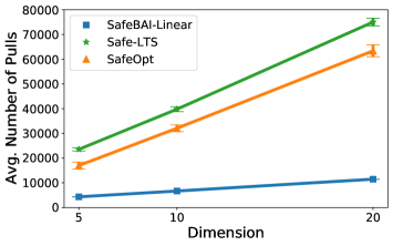
Figure 1: Total arm pulls to termination vs. dimension in the linear model. Error bars give 1 standard deviation.

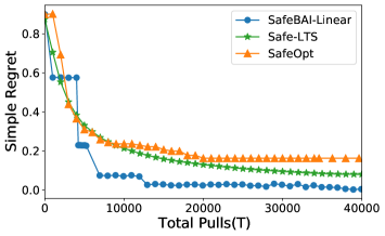
Figure 2: Simple regret in linear model with $d=10$.

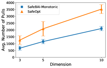
Figure 3: Total arm pulls to termination vs. dimension in drug response model. Error bars give 1 standard deviation.

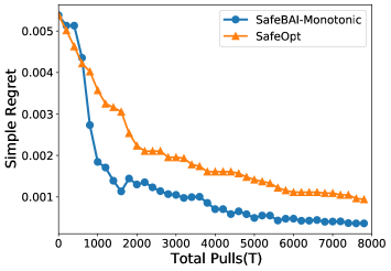
Figure 4: Simple regret in drug response model with $d=20$.

7.3 Application to Best Drug Identification

In the second experiment, we investigate the performance of SafeBAI-Monotonic in comparison to SafeOpt on a nonlinear drug response model. In the dose-finding literature, it is often assumed that higher dosage leads to stronger drug response and efficacy, while also increasing toxicity (Mandrekar et al., 2007; Yuan & Yin, 2009; Cai et al., 2014). A common assumption (see e.g. Thall & Russell (1998) and aforementioned works) has been to rely on a logistic function to model both the efficacy and toxicity: for the $i$th drug and dose $a$, the efficacy is modeled as $f_{i}(a)=\frac{1}{1+e^{-\theta_{i}\cdot a}}$ and toxicity as $g_{i}(a)=\frac{1}{1+e^{-\mu_{i}\cdot a}}$. Note that this choice of $f_{i}$ and $g_{i}$ is monotonic and fits within our setting. Applying this model, we can effectively consider a drug selection setup where our goal is to identify the drug with highest utility among a set of candidate drugs, while ensuring none of the dosages tested lead to toxic response, i.e. all drug tests satisfy a safety constraint. We design drug sets with a number of $d\in\{3,5,10,20\}$ drugs, efficacy model parameters $\theta_{1}=0.01,\theta_{i>1}=10$, toxicity model parameters $\mu_{i}=1$. This gives a minimum gap $\Delta\approx 0.497$. The safety threshold $\gamma$ is set to 0.3. For SafeOpt, we use an RBF kernel. The sample observations are perturbed by Gaussian noise with mean 0 and variance $\sigma^{2}=0.1$. Similar to the linear case, we will also plot the simple regret values, where here we define the simple regret as $r_{t}=f_{i^{*}}(a_{i^{*}})-f_{\widehat{i}_{t}}(\widehat{a}_{s}^{t}(\widehat{i}_{t}))$, for $\widehat{i}_{t}=\ \operatorname*{arg\,max}_{i}\widehat{f}_{i}(\widehat{a}_{s}^{t}(i)).$ We run SafeOpt with an RBF kernel in this setting. All data points are the average of 20 trials.

The result in Figure 3 suggests SafeBAI-Monotonic is able to much more effectively identify the best safe drug than SafeOpt. The total number of drug evaluations required for SafeBAI-Monotonic is roughly half of SafeOpt in all instances. Furthermore, the expensive posterior update in SafeOpt makes it slow to run with samples $>5000$, while SafeBAI-Monotonic can be efficiently run when many more samples are required, allowing it to easily scale to trials with more drugs. Figure 4 illustrates that SafeBAI-Monotonic also performs much better in terms of the simple regret. Not only is it able to identify and verify the optimal coordinate more quickly, even before verifying it has found the optimal coordinate, its sampling strategy allows it to obtain better intermediate estimates of the best coordinate.

Acknowledgements

The work of AW is supported by an NSF GFRP Fellowship DGE-1762114. The work of KJ is supported in part by grants NSF CCF 2007036 and NSF TRIPODS 2023166.

Appendix A Linear Response Functions Proof

A.1 Correctness of SafeBAI-Linear

Lemma 1.

For any $i\in[d]$ and $\ell\in\mathbb{N}^{+}$, define the events

$$\mathcal{E}_{i,\ell}(\theta)=\left\{|\widehat{\theta}_{i,\ell}-\theta_{i}|\leq\frac{2^{-\ell}}{\widehat{a}_{s}^{\ell-1}(i)}\right\},\quad\mathcal{E}_{i,\ell}(\mu)=\left\{|\widehat{\mu}_{i,\ell}-\mu_{i}|\leq\frac{2^{-\ell}}{\widehat{a}_{s}^{\ell-1}(i)}\right\}$$ (1)

and let

$$\mathcal{E}:=\left(\bigcap_{i=1}^{d}\bigcap_{\ell=1}^{\infty}\mathcal{E}_{i,\ell}(\theta)\right)\cap\left(\bigcap_{i=1}^{d}\bigcap_{\ell=1}^{\infty}\mathcal{E}_{i,\ell}(\mu)\right).$$

Then it holds that $\mathbb{P}(\mathcal{E})\geq 1-\delta$.

Proof of Lemma 1.

Given that at $\ell$-th iteration, $N_{\ell}=\lceil 2\sigma^{2}\log\frac{8d\ell^{2}}{\delta}\cdot\epsilon_{\ell}^{-2}\rceil$ and

$$\widehat{a}_{s}^{\ell-1}(i)\widehat{\theta}_{i,\ell}=\frac{1}{N_{\ell}}\sum_{t=1}^{n_{i}}(\widehat{a}_{s}^{\ell-1}(i)\theta_{i}+\eta_{t})=\widehat{a}_{s}^{\ell-1}(i)\theta_{i}+\frac{1}{n_{i}}\sum_{t=1}^{N_{\ell}}\eta_{t}.$$

By Hoeffding’s inequality, $|\widehat{a}_{s}^{\ell-1}(i)\theta_{i}-\widehat{a}_{s}^{\ell-1}(i)\widehat{\theta}_{i,\ell}|\leq\sqrt{\frac{2\sigma^{2}\log(\frac{8d\ell^{2}}{\delta})}{N_{\ell}}}=2^{-\ell}$ with probability $1-\frac{\delta}{4d\ell^{2}}$. Thus we have that $\mathbb{P}(\mathcal{E}^{c}_{i,\ell}(\theta))=\mathbb{P}(\mathcal{E}^{c}_{i,\ell}(\mu))\leq\frac{\delta}{4d\ell^{2}}$. Taking union bound over all coordinates and rounds we have:

$$\mathbb{P}(\bigcup^{d}_{i=1}\bigcup^{\infty}_{\ell=1}\mathcal{E}^{c}_{i,\ell}(\mu))\leq\sum^{d}_{i=1}\sum^{\infty}_{\ell=1}\frac{\delta}{4d\ell^{2}}=d\cdot\frac{\delta}{4d}\cdot\frac{\pi^{2}}{6}\leq\delta/2.$$ (2)

Using the same inequality on the union bound we can obtain the inequality result for $\theta$ as well, and union bounding over both gives the result. ∎

Lemma 2.

On the event $\mathcal{E}$, for all $\ell$ and $i\in\mathcal{X}_{\ell-1}$, we will have that $\widehat{a}_{s}^{\ell}(i)\in\mathcal{S}_{i}$.

Proof.

On the event $\mathcal{E}$, $|\widehat{\mu}_{i,\ell}-\mu_{i}|\leq\frac{2^{-\ell}}{\widehat{a}_{s}^{\ell-1}(i)},|\widehat{\theta}_{i,\ell}-\theta_{i}|\leq\frac{2^{-\ell}}{\widehat{a}_{s}^{\ell-1}(i)}$. Then using our choice of $\widehat{a}_{s}^{\ell}(i)$, it follows that $\widehat{a}_{s}^{\ell}(i)\mu_{i}\leq\widehat{a}_{s}^{\ell}(i)(\widehat{\mu}_{i,\ell}+\tfrac{\epsilon_{\ell}}{\widehat{a}_{s}^{\ell-1}(i)})=\gamma$. Thus, by construction, $\widehat{a}_{s}^{\ell}(i)$ will be safe. ∎

Lemma 3.

On the event $\mathcal{E}$, coordinate $i$ is suboptimal if the event

$$\{\exists j\in[n],\ell>0:\widehat{a}_{u}^{\ell}(i)(\widehat{\theta}_{i,\ell}+\frac{2^{-\ell}}{\widehat{a}_{s}^{\ell-1}(i)})<\widehat{a}_{s}^{\ell}(j)(\widehat{\theta}_{j,\ell}-\frac{2^{-\ell}}{\widehat{a}_{s}^{\ell-1}(j)})\}$$ (3)

holds, so $i^{*}\in\mathcal{X}_{\ell}$ for all $\ell$.

Proof of Lemma 3.

Fix coordinate $i$ and its largest safe value $a_{s}(i)$. By Lemma 2, we will have that $\widehat{a}_{s}^{\ell}(i)$ is safe. Further, applying our choice of $\widehat{a}_{u}^{\ell}(i)$, we obtain

$$\widehat{a}_{s}^{\ell}(i)=M_{i}\wedge\gamma/(\widehat{\mu}_{i,\ell}+\tfrac{\epsilon_{\ell}}{\widehat{a}_{s}^{\ell-1}(i)})\leq a_{s}(i)=M_{i}\wedge\gamma/\mu_{i}\leq M_{i}\wedge\gamma/(\widehat{\mu}_{i,\ell}-\tfrac{\epsilon_{\ell}}{\widehat{a}_{s}^{\ell-1}(i)})=\widehat{a}_{u}^{\ell}(i).$$

Applying this set of inequalities $\widehat{a}_{s}^{\ell}(i)\leq a_{s}(i)\leq\widehat{a}_{u}^{\ell}(i)$, it follows that

$$\widehat{a}_{u}^{\ell}(i)(\widehat{\theta}_{i,\ell}+\frac{2^{-\ell}}{\widehat{a}_{s}^{\ell-1}(i)})<\widehat{a}_{s}^{\ell}(j)(\widehat{\theta}_{j,\ell}-\frac{2^{-\ell}}{\widehat{a}_{s}^{\ell-1}(j)})$$

$$\implies a_{s}(i)(\widehat{\theta}_{i,\ell}+\frac{2^{-\ell}}{\widehat{a}_{s}^{\ell-1}(i)})<\widehat{a}_{s}^{\ell}(j)(\widehat{\theta}_{j,\ell}-\frac{2^{-\ell}}{\widehat{a}_{s}^{\ell-1}(j)})$$

$$\implies a_{s}(i)\theta_{i}<a_{s}(j)\theta_{j}.$$

The last inequality suggests $i$ being suboptimal by definition. That $i^{*}\in\mathcal{X}_{\ell}$ for all $\ell$ follows directly since (3) is identical to the condition in Algorithm 1 to remove a coordinate, and so, since (3) implies $i$ is suboptimal, it follows that $i^{*}$ can never be removed. ∎

A.2 Coordinate Elimination Criteria

Lemma 4.

Assume $\widehat{a}_{s}^{\ell}(i)<M_{i}$ and $\widehat{a}_{s}^{\ell}(i^{*})<M_{i^{*}}$ and that $\mathcal{E}$ holds. Let $\underline{a}(i,\ell)$ be a lower bound for $\widehat{a}_{s}^{\ell}(i)$, then any suboptimal coordinate $i$ will be eliminated after the $\ell$-th iteration where $\ell$ satisfies:

$$\frac{\theta_{i}\underline{a}(i,\ell-1)+2^{1-\ell}}{\mu_{i}\underline{a}(i,\ell-1)-2^{1-\ell}}\leq\frac{\theta_{i^{*}}\underline{a}(i^{*},\ell-1)-2^{1-\ell}}{\mu_{i^{*}}\underline{a}(i^{*},\ell-1)+2^{1-\ell}}.$$ (4)

Proof of Lemma 4.

Since on $\mathcal{E}$, $i^{*}\in\mathcal{X}_{\ell}$ for all $\ell$ as shown in Lemma 3, a sufficient condition to eliminate coordinate $i$ is that $i^{*}$ has a larger estimated maximum safe value, and we can therefore reduce the elimination criteria to simply a comparison between $i$ and $i^{*}$. First we transform this inequality via:

$$\frac{\theta_{i}\underline{a}(i,\ell-1)+2^{1-\ell}}{\mu_{i}\underline{a}(i,\ell-1)-2^{1-\ell}}\leq\frac{\theta_{i^{*}}\underline{a}(i^{*},\ell-1)-2^{1-\ell}}{\mu_{i^{*}}\underline{a}(i^{*},\ell-1)+2^{1-\ell}}\implies\frac{\gamma(\theta_{i}+\frac{2^{1-\ell}}{\underline{a}(i,\ell-1)})}{\mu_{i}-\frac{2^{1-\ell}}{\underline{a}(i,\ell-1)}}\leq\frac{\gamma(\theta_{i^{*}}-\frac{2^{1-\ell}}{\underline{a}(i^{*},\ell-1)})}{\mu_{i^{*}}+\frac{2^{1-\ell}}{\underline{a}(i^{*},\ell-1)}}$$ (5)

Note that, by their definition and on $\mathcal{E}$, $\widehat{a}_{s}^{\ell}(i^{*})\geq\frac{\gamma}{\mu_{i^{*}}+\frac{2^{1-\ell}}{\underline{a}(i^{*},\ell-1)}}$, $\widehat{a}_{u}^{\ell}(i)\leq\frac{\gamma}{\mu_{i}-\frac{2^{1-\ell}}{\underline{a}(i,\ell-1)}}$. Using this and that $\underline{a}(i,\ell)\leq\widehat{a}_{s}^{\ell}(i)$ and $|\widehat{\theta}_{i,\ell}-\theta_{i}|\leq\frac{2^{-\ell}}{\widehat{a}_{s}^{\ell-1}(i)}$, we have that (5) implies:

$$\widehat{a}_{u}^{\ell}(i)(\theta_{i}+\frac{2^{1-\ell}}{\underline{a}(i,\ell-1)})<\widehat{a}_{s}^{\ell}(i^{*})(\theta_{i^{*}}-\frac{2^{1-\ell}}{\underline{a}(i^{*},\ell-1)})$$

$$\implies\widehat{a}_{u}^{\ell}(i)(\theta_{i}+2\frac{2^{-\ell}}{\widehat{a}_{s}^{\ell-1}(i)})<\widehat{a}_{s}^{\ell}(i^{*})(\theta_{i^{*}}-2\frac{2^{-\ell}}{\widehat{a}_{s}^{\ell-1}(i^{*})})$$

$$\implies\widehat{a}_{u}^{\ell}(i)(\widehat{\theta}_{i,\ell}+\frac{2^{-\ell}}{\widehat{a}_{s}^{\ell-1}(i)})<\widehat{a}_{s}^{\ell}(i^{*})(\widehat{\theta}_{i^{*},\ell}-\frac{2^{-\ell}}{\widehat{a}_{s}^{\ell-1}(i^{*})})$$

From the last inequality and Lemma 3, we have that $i$ stops getting sampled at such $\ell$. ∎

Lemma 5.

On $\mathcal{E}$, for any saturated coordinate $i$ (i.e. $a_{s}(i)=M_{i}$), when $i^{*}$ is not saturated, we will eliminate $i$ after the $\ell$-th iteration when $\ell$ satisfies:

$$M_{i}\theta_{i}+2^{1-\ell}<\gamma\cdot\frac{\theta_{i^{*}}\underline{a}({i^{*}},\ell-1)-2^{1-\ell}}{\mu_{i^{*}}\underline{a}({i^{*}},\ell-1)+2^{1-\ell}}$$ (6)

Proof of Lemma 5.

Since on $\mathcal{E}$, $i^{*}\in\mathcal{X}_{\ell}$ for all $\ell$ as shown in Lemma 3, a sufficient condition to eliminate coordinate $i$ is that $i^{*}$ has a larger estimated maximum safe value, and we can therefore reduce the elimination criteria to simply a comparison between $i$ and $i^{*}$. First we transform this inequality via:

$$M_{i}\theta_{i}+2^{1-\ell}<\gamma\cdot\frac{\theta_{i^{*}}\underline{a}({i^{*}},\ell-1)-2^{1-\ell}}{\mu_{i^{*}}\underline{a}({i^{*}},\ell-1)+2^{1-\ell}}\implies M_{i}(\theta_{i}+\frac{2^{1-\ell}}{M_{i}})<\frac{\gamma\cdot(\theta_{i^{*}}-\frac{2^{1-\ell}}{\underline{a}({i^{*}},\ell-1)})}{\mu_{i^{*}}+\frac{2^{1-\ell}}{\underline{a}({i^{*}},\ell-1)}}$$ (7)

Note that $\widehat{a}_{s}^{\ell}(i)=M_{i}=\widehat{a}_{s}^{\ell-1}(i)$, $\widehat{a}_{s}^{\ell}(i^{*})\geq\frac{\gamma}{\mu_{i^{*}}+\frac{2^{1-\ell}}{\underline{a}(i^{*},\ell-1)}}$. Using $\underline{a}(i,\ell)\leq\widehat{a}_{s}^{\ell}(i)$ and $|\widehat{\theta}_{i,\ell}-\theta_{i}|\leq\frac{2^{-\ell}}{\widehat{a}_{s}^{\ell-1}(i)}$, we have that (7) implies:

$$M_{i}(\theta_{i}+\frac{2^{1-\ell}}{M_{i}})<\widehat{a}_{s}^{\ell}(i^{*})(\theta_{i^{*}}-2\frac{2^{-\ell}}{\widehat{a}_{s}^{\ell-1}(i^{*})})$$

$$\implies\widehat{a}_{u}^{\ell}(i)(\theta_{i}+2\frac{2^{-\ell}}{\widehat{a}_{s}^{\ell-1}(i)})<\widehat{a}_{s}^{\ell}(i^{*})(\theta_{i^{*}}-2\frac{2^{-\ell}}{\widehat{a}_{s}^{\ell-1}(i^{*})})$$

$$\implies\widehat{a}_{u}^{\ell}(i)(\widehat{\theta}_{i,\ell}+\frac{2^{-\ell}}{\widehat{a}_{s}^{\ell-1}(i)})<\widehat{a}_{s}^{\ell}(i^{*})(\widehat{\theta}_{i^{*},\ell}-\frac{2^{-\ell}}{\widehat{a}_{s}^{\ell-1}(i^{*})}).$$

From the last inequality and Lemma 3, we have that $i$ stops getting sampled at such $\ell$. ∎

Lemma 6.

On $\mathcal{E}$, when $i^{*}$ is a saturated coordinate (i.e. $a_{s}(i^{*})=M_{i^{*}}$), then for any unsaturated suboptimal coordinate $i$, we will eliminate $i$ after the $\ell$-th iteration where $\ell$ satisfies:

$$\gamma\cdot\frac{\theta_{i}\underline{a}(i,\ell-1)+2^{1-\ell}}{\mu_{i}\underline{a}(i,\ell-1)-2^{1-\ell}}<M_{i^{*}}\theta_{i^{*}}-2^{1-\ell}$$ (8)

Proof of Lemma 6.

Since on $\mathcal{E}$, $i^{*}\in\mathcal{X}_{\ell}$ for all $\ell$ as shown in Lemma 3, a sufficient condition to eliminate coordinate $i$ is that $i^{*}$ has a larger estimated maximum safe value, and we can therefore reduce the elimination criteria to simply a comparison between $i$ and $i^{*}$. First we transform this inequality via:

$$\gamma\cdot\frac{\theta_{i}\underline{a}(i,\ell-1)+2^{1-\ell}}{\mu_{i}\underline{a}(i,\ell-1)-2^{1-\ell}}<M_{i^{*}}\theta_{i^{*}}-2^{1-\ell}\implies\frac{\gamma\cdot(\theta_{i}+\frac{2^{1-\ell}}{\underline{a}(i,\ell-1)})}{\mu_{i}-\frac{2^{1-\ell}}{\underline{a}(i,\ell-1)}}<M_{i^{*}}(\theta_{i^{*}}-\frac{2^{1-\ell}}{M_{i^{*}}})$$ (9)

Note that $\widehat{a}_{s}^{\ell}(i^{*})=M_{i^{*}}=\widehat{a}_{s}^{\ell-1}(i^{*})$, $\widehat{a}_{u}^{\ell}(i)\leq\frac{\gamma}{\mu_{i}-\frac{2^{1-\ell}}{\underline{a}(i,\ell-1)}}$. Using $\underline{a}(i,\ell)\leq\widehat{a}_{s}^{\ell}(i)$ and $|\widehat{\theta}_{i,\ell}-\theta_{i}|\leq\frac{2^{-\ell}}{\widehat{a}_{s}^{\ell-1}(i)}$, we have (9) implies:

$$\widehat{a}_{u}^{\ell}(i)(\theta_{i}+\frac{2^{1-\ell}}{\underline{a}(i,\ell-1)})<M_{i^{*}}(\theta_{i^{*}}-\frac{2^{1-\ell}}{M_{i^{*}}})$$

$$\implies\widehat{a}_{u}^{\ell}(i)(\theta_{i}+2\frac{2^{-\ell}}{\widehat{a}_{s}^{\ell-1}(i)})<\widehat{a}_{s}^{\ell}(i^{*})(\theta_{i^{*}}-2\frac{2^{-\ell}}{\widehat{a}_{s}^{\ell-1}(i^{*})})$$

$$\implies\widehat{a}_{u}^{\ell}(i)(\widehat{\theta}_{i,\ell}+\frac{2^{-\ell}}{\widehat{a}_{s}^{\ell-1}(i)})<\widehat{a}_{s}^{\ell}(i^{*})(\widehat{\theta}_{i^{*},\ell}-\frac{2^{-\ell}}{\widehat{a}_{s}^{\ell-1}(i^{*})})$$

From the last inequality and Lemma 3, we have that $i$ stops getting sampled at such $\ell$. ∎

A.3 Lower Bounding Safe Value Estimate

Lemma 7.

Define

$$\underline{a}_{s}^{\ell}(i):=\frac{\gamma^{\ell}2^{\ell(\ell+1)/2}}{\mu_{i}\sum^{\ell}_{k=1}2^{\ell-k}\gamma^{k-1}2^{k(k+1)/2}+\frac{2^{\ell}}{a_{0,i}}}.$$

Let $\ell_{0}:=\operatorname*{arg\,min}_{\ell}\ell\text{ s.t. }\underline{a}_{s}^{\ell}(i)\geq M_{i}$. Then, on $\mathcal{E}$:

$$\widehat{a}_{s}^{\ell}(i)\geq\left\{\begin{matrix}\min\{\max\{\underline{a}_{s}^{\ell}(i),\ a_{0,i}\},M_{i}\}&\ell<\ell_{0}\\ M_{i}&\ell\geq\ell_{0}\end{matrix}\right..$$

Proof of Lemma 7.

Recall our choice of $\widehat{a}_{s}^{\ell}(i)=\min\{\max\{\gamma/(\widehat{\mu}_{i,\ell}+\frac{2^{-\ell}}{\widehat{a}_{s}^{\ell-1}(i)}),a_{0,i}\},M_{i}\}$. Let $\ell_{0}:=\operatorname*{arg\,min}_{\ell}\ell\text{ s.t. }\underline{a}_{s}^{\ell}(i)\geq M_{i}$. We will first show that for $\ell<\ell_{0}$, we can lower bound $\widehat{a}_{s}^{\ell}(i)\geq\max\{\underline{a}_{s}^{\ell}(i),\ a_{0,i}\}$. We prove this lemma via induction.

In the base case, since on $\mathcal{E}$, $|\widehat{\mu}_{i,\ell}-\mu_{i}|\leq\frac{2^{-\ell}}{\widehat{a}_{s}^{\ell-1}(i)}$, we have

$$\widehat{a}_{s}^{1}(i)=\max\{\frac{\gamma}{\widehat{\mu}_{i,1}+\frac{2^{-1}}{a_{0,i}}},a_{0,i}\}\geq\max\{\frac{\gamma^{1}}{\mu_{i}+2\frac{2^{-1}}{a_{0,i}}},a_{0,i}\}=\max\{\frac{\gamma^{1}\cdot 2}{2\mu_{i}+\frac{2}{a_{0,i}}},a_{0,i}\}=\max\{\underline{a}_{s}^{\ell}(i),a_{0,i}\},$$

hence the base case holds. Next, suppose the inequality holds for $\ell-1$, i.e. $\widehat{a}_{s}^{\ell-1}(i)\geq\max\{\underline{a}_{s}^{\ell-1}(i),a_{0,i}\}$, then we obtain, on $\mathcal{E}$,

$$\frac{\gamma}{\widehat{\mu}_{i,\ell}+\frac{2^{-\ell}}{\widehat{a}_{s}^{\ell-1}(i)}} \geq\frac{\gamma}{\mu_{i}+2\cdot\frac{2^{-\ell}}{\widehat{a}_{s}^{\ell-1}(i)}}$$

$$=\frac{\gamma}{\mu_{i}+2\cdot\frac{2^{-\ell}}{\max\{\gamma/(\widehat{\mu}_{i,\ell-1}+\frac{2^{1-\ell}}{\widehat{a}_{s}^{\ell-2}(i)}),a_{0,i}\}}}$$

$$\geq\frac{\gamma}{\mu_{i}+2\cdot\frac{2^{-\ell}}{\gamma/(\widehat{\mu}_{i,\ell-1}+\frac{2^{1-\ell}}{\widehat{a}_{s}^{\ell-2}(i)})}}$$

$$\geq\frac{\gamma}{\mu_{i}+2\cdot 2^{-\ell}\frac{\mu_{i}\sum^{\ell-1}_{k=1}2^{\ell-1-k}\gamma^{k-1}2^{\sum^{k}_{s=1}s}+\frac{2^{\ell-1}}{a_{0,i}}}{\gamma^{\ell-1}2^{\sum^{\ell-1}_{k=1}k}}}$$

$$=\frac{\gamma\cdot\gamma^{\ell-1}2^{\sum^{\ell-1}_{k=1}k}}{\mu_{i}\cdot\gamma^{\ell-1}2^{\sum^{\ell-1}_{k=1}k}+2\cdot 2^{-\ell}(\mu_{i}\sum^{\ell-1}_{k=1}2^{\ell-1-k}\gamma^{k-1}2^{\sum^{k}_{s=1}s}+\frac{2^{\ell-1}}{a_{0,i}})}$$

$$=\frac{\gamma^{\ell}2^{\sum^{\ell-1}_{k=1}k}2^{\ell}}{\mu_{i}\cdot\gamma^{\ell-1}2^{\sum^{\ell-1}_{k=1}k}2^{\ell}+2\mu_{i}\sum^{\ell-1}_{k=0}2^{\ell-1-k}\gamma^{k-1}2^{\sum^{k}_{s=1}s}+\frac{2^{\ell}}{a_{0,i}}}$$

$$=\frac{\gamma^{\ell}2^{\sum^{\ell}_{k=1}k}}{\mu_{i}\sum^{\ell}_{k=1}2^{\ell-k}\gamma^{k-1}2^{\sum^{k}_{s=1}s}+\frac{2^{\ell}}{a_{0,i}}}.$$

Since $\sum^{k}_{s=1}s=s(s+1)/2$, it follows then that

$$\widehat{a}_{s}^{\ell}(i) =\min\bigg{\{}\max\bigg{\{}\frac{\gamma}{\widehat{\mu}_{i,\ell}+\frac{2^{1-\ell}}{\widehat{a}_{s}^{\ell-1}(i)}},a_{0,i}\bigg{\}},M_{i}\bigg{\}}\geq\min\{\max\{\underline{a}_{s}^{\ell}(i),a_{0,i}\},M_{i}\}.$$

Since $\ell<\ell_{0}$, by definition $\underline{a}_{s}^{\ell}(i)<M_{i}$, which implies that $\max\{\underline{a}_{s}^{\ell}(i),a_{0,i}\}\leq M_{i}$ (since $a_{0,i}\leq M_{i}$ by assumption), so $\widehat{a}_{s}^{\ell}(i)\geq\max\{\underline{a}_{s}^{\ell}(i),a_{0,i}\}$, proving the inductive step. We conclude that for any $\ell<\ell_{0}$, we can lower bound $\widehat{a}_{s}^{\ell}(i)\geq\max\{\underline{a}_{s}^{\ell}(i),a_{0,i}\}=\min\{\max\{\underline{a}_{s}^{\ell}(i),a_{0,i}\},M_{i}\}$.

Now take $\ell=\ell_{0}$. In this case we can use that $\widehat{a}_{s}^{\ell_{0}-1}(i)\geq\max\{\underline{a}_{s}^{\ell_{0}-1}(i),a_{0,i}\}$ and repeat the above calculation to get that

$$\frac{\gamma}{\widehat{\mu}_{i,\ell_{0}}+\frac{2^{1-\ell_{0}}}{\widehat{a}_{s}^{\ell_{0}-1}(i)}}\geq\underline{a}_{s}^{\ell_{0}}(i).$$

Since by definition $\underline{a}_{s}^{\ell_{0}}(i)\geq M_{i}$, we conclude

$$\widehat{a}_{s}^{\ell_{0}}(i) =\min\bigg{\{}\max\bigg{\{}\frac{\gamma}{\widehat{\mu}_{i,\ell_{0}}+\frac{2^{1-\ell_{0}}}{\widehat{a}_{s}^{\ell_{0}-1}(i)}},a_{0,i}\bigg{\}},M_{i}\bigg{\}}\geq\min\{\max\{\underline{a}_{s}^{\ell_{0}}(i),a_{0,i}\},M_{i}\}\geq\min\{\max\{M_{i},a_{0,i}\},M_{i}\}=M_{i}.$$

Since we set $\widehat{a}_{s}^{\ell}(i)$ to $M_{i}$ for all epochs after the first epoch for which $\widehat{a}_{s}^{\ell}(i)=M_{i}$, it follows that $\widehat{a}_{s}^{\ell}(i)=M_{i}$ for $\ell\geq\ell_{0}$. ∎

Lemma 8.

We will have that

$$\underline{a}_{s}^{\ell}(i):=\frac{\gamma^{\ell}2^{\ell(\ell+1)/2}}{\mu_{i}\sum^{\ell}_{k=1}2^{\ell-k}\gamma^{k-1}2^{k(k+1)/2}+\frac{2^{\ell}}{a_{0,i}}}\geq\frac{\gamma}{(1+\alpha)\mu_{i}}$$

as long as

$$\ell\geq\Phi_{i}(\alpha):=\max\left\{8,\sqrt{8\log_{2}\frac{2\gamma}{\alpha}},\sqrt{4\log_{2}\frac{2\gamma}{a_{0,i}\mu_{i}\alpha}},4\log_{2}\frac{2^{1/2}}{\gamma},\log_{2}\frac{4}{\gamma\alpha}+2\log_{2}\left(\log_{2}\frac{4}{\gamma\alpha}\right)\right\}.$$

Proof.

We first want to find a lower bound on $\ell$ that will guarantee

$$2^{\ell}/a_{0,i}\leq\frac{\alpha}{2}\cdot\mu_{i}\gamma^{\ell-1}2^{\ell(\ell+1)/2}$$ (10)

since in this case we can lower bound

$$\frac{\gamma^{\ell}2^{\ell(\ell+1)/2}}{\mu_{i}\sum^{\ell}_{k=1}2^{\ell-k}\gamma^{k-1}2^{k(k+1)/2}+\frac{2^{\ell}}{a_{0,i}}} \geq\frac{\gamma^{\ell}2^{\ell(\ell+1)/2}}{\mu_{i}\sum^{\ell}_{k=1}2^{\ell-k}\gamma^{k-1}2^{k(k+1)/2}+\frac{\alpha}{2}\cdot\mu_{i}\gamma^{\ell-1}2^{\ell(\ell+1)/2}}$$

$$=\frac{\gamma}{\mu_{i}}\cdot\frac{1}{\sum^{\ell}_{k=1}\frac{2^{\ell-k}\gamma^{k-1}2^{k(k+1)/2}}{\gamma^{\ell-1}2^{\ell(\ell+1)/2}}+\alpha/2}.$$

To show (10), we can rearrange it as

$$(2^{1/2}/\gamma)^{\ell}\leq\frac{a_{0,i}\mu_{i}\alpha}{2\gamma}2^{\ell^{2}/2}.$$

Note that $(2^{1/2}/\gamma)^{\ell}\leq 2^{\ell^{2}/4}$ for

$$\ell\geq 4\log_{2}(2^{1/2}/\gamma).$$

So for $\ell$ satisfying this, we will have that $(2^{1/2}/\gamma)^{\ell}\leq\frac{a_{0,i}\mu_{i}\alpha}{2\gamma}2^{\ell^{2}/2}$ as long as

$$2^{\ell^{2}/4}\leq\frac{a_{0,i}\mu_{i}\alpha}{2\gamma}2^{\ell^{2}/2}\implies\frac{2\gamma}{a_{0,i}\mu_{i}\alpha}\leq 2^{\ell^{2}/4}\implies\sqrt{4\log_{2}\frac{2\gamma}{a_{0,i}\mu_{i}\alpha}}\leq\ell$$

so a sufficient condition to meet (10) is

$$\ell\geq\max\left\{\sqrt{4\log_{2}\frac{2\gamma}{a_{0,i}\mu_{i}\alpha}},4\log_{2}\frac{2^{1/2}}{\gamma}\right\}.$$

Our goal now is to find $\ell$ such that

$$1+\frac{\alpha}{2}\geq\sum^{\ell}_{k=1}\frac{2^{\ell-k}\gamma^{k-1}2^{k(k+1)/2}}{\gamma^{\ell-1}2^{\ell(\ell+1)/2}}=1+\sum^{\ell-1}_{k=1}\frac{2^{\ell-k}\gamma^{k-1}2^{k(k+1)/2}}{\gamma^{\ell-1}2^{\ell(\ell+1)/2}}.$$

If we can find such an $\ell$, the desired conclusion will follow. Note that

$$2^{\ell-k}\gamma^{k-1}2^{k(k+1)/2}\leq\max\{2^{\ell},2\gamma^{\ell-2}2^{\frac{(\ell-1)\ell}{2}}\},\quad\forall k\leq\ell-1.$$ (11)

To see this, consider

$$\log_{2}(2^{\ell-k}\gamma^{k-1}2^{k(k+1)/2})=\ell-k+(k-1)\log_{2}\gamma+k^{2}/2+k/2.$$

Taking the derivative of this with respect to $k$ we get

$$-1/2+\log_{2}\gamma+k.$$

As this is negative for $k<1/2-\log_{2}\gamma$ and otherwise positive, it follows that the maximum of $2^{\ell-k}\gamma^{k-1}2^{k(k+1)/2}$ over the range $k\in[1,\ell-1]$ must either occur at $k=1$, or $k=\ell-1$.

It follows that

$$\sum^{\ell-1}_{k=1}\frac{2^{\ell-k}\gamma^{k-1}2^{k(k+1)/2}}{\gamma^{\ell-1}2^{\ell(\ell+1)/2}}\leq\frac{(\ell-1)\max\{2^{\ell},2\gamma^{\ell-2}2^{\frac{(\ell-1)\ell}{2}}\}}{\gamma^{\ell-1}2^{\ell(\ell+1)/2}}=(\ell-1)\max\{\gamma^{1-\ell}2^{\ell/2-\ell^{2}/2},\gamma^{-1}2^{1-\ell}\}.$$

Now

$$(\ell-1)\gamma^{-1}2^{1-\ell}\leq\alpha/2\iff\log_{2}(\ell-1)-\log_{2}\frac{\gamma\alpha}{4}\leq\ell.$$

Assume that $-\log_{2}\frac{\gamma\alpha}{4}>0$, as otherwise we are trivially done. We claim that the above inequality is satisfied as long as

$$\ell\geq\max\{-\log_{2}\frac{\gamma\alpha}{4},3\}+2\log\left(\max\{-\log_{2}\frac{\gamma\alpha}{4},3\}\right).$$

To see this, note that with $\ell=\max\{-\log_{2}\frac{\gamma\alpha}{4},3\}+2\log\left(\max\{-\log_{2}\frac{\gamma\alpha}{4},3\}\right)$, we have

$$\log_{2}(\ell-1)-\log_{2}\frac{\gamma\alpha}{4} =\log_{2}\left(\max\{-\log_{2}\frac{\gamma\alpha}{4},3\}+2\log\left(\max\{-\log_{2}\frac{\gamma\alpha}{4},3\}\right)-1\right)-\log_{2}\frac{\gamma\alpha}{4}$$

$$\leq\log_{2}\left(3\max\{-\log_{2}\frac{\gamma\alpha}{4},3\}\right)-\log_{2}\frac{\gamma\alpha}{4}$$

$$\leq\max\{-\log_{2}\frac{\gamma\alpha}{4},3\}+2\log\left(\max\{-\log_{2}\frac{\gamma\alpha}{4},3\}\right)$$

$$=\ell$$

where the last inequality follows since

$$\log_{2}\left(3\max\{-\log_{2}\frac{\gamma\alpha}{4},3\}\right) =\log_{2}3+\log_{2}\left(\max\{-\log_{2}\frac{\gamma\alpha}{4},3\}\right)$$

$$\leq 2\log_{2}\left(\max\{-\log_{2}\frac{\gamma\alpha}{4},3\}\right).$$

To guarantee that

$$(\ell-1)\gamma^{1-\ell}2^{\ell/2-\ell^{2}/2}\leq\alpha/2\iff\log_{2}(\ell-1)+\ell\log_{2}(2^{1/2}/\gamma)-\log_{2}\frac{\alpha}{2\gamma}\leq\ell^{2}/2$$

it suffices to take

$$\ell\geq\max\{8,\sqrt{-8\log_{2}\frac{\alpha}{2\gamma}},4\log_{2}\frac{2^{1/2}}{\gamma}\}.$$

Putting all of this together, we have shown that

$$\frac{\gamma^{\ell}2^{\ell(\ell+1)/2}}{\mu_{i}\sum^{\ell}_{k=1}2^{\ell-k}\gamma^{k-1}2^{k(k+1)/2}+\frac{2^{\ell}}{a_{0,i}}}\geq\frac{\gamma}{(1+\alpha)\mu_{i}}$$

as long as

$$\ell\geq\max\left\{8,\sqrt{-8\log\frac{\alpha}{2\gamma}},\sqrt{4\log_{2}\frac{2\gamma}{a_{0,i}\mu_{i}\alpha}},4\log_{2}\frac{2^{1/2}}{\gamma},\max\{-\log_{2}\frac{\gamma\alpha}{4},3\}+2\log\left(\max\{-\log_{2}\frac{\gamma\alpha}{4},3\}\right)\right\}.$$

Note that if $\max\{-\log_{2}\frac{\gamma\alpha}{4},3\}=3$, then the condition

$$\ell\geq\max\{-\log_{2}\frac{\gamma\alpha}{4},3\}+2\log\left(\max\{-\log_{2}\frac{\gamma\alpha}{4},3\}\right)$$

is implied by $\ell\geq 8$. The stated conclusion follows. ∎

A.4 Sample Complexity of SafeBAI-Linear

We will define the following:

$$\Psi^{1}_{i}(x) :=\log_{2}\frac{4(2+\frac{\theta_{i^{*}}}{\mu_{i^{*}}}+\frac{\theta_{i}}{\mu_{i}})}{x}$$

$$\Psi^{2}_{i}(x) :=\max\left\{\log_{2}\frac{4(2+M_{i}\theta_{i}/\gamma)}{x},\log_{2}\frac{4}{\gamma}\right\}$$

$$\Psi^{3}_{i}(x) :=\log_{2}\frac{4}{x}$$

$$\alpha_{i} :=\frac{\gamma}{\mu_{i}M_{i}}-1$$

Lemma 9.

On $\mathcal{E}$, when running Algorithm 1:

1. If $M_{i}\not\in\mathcal{S}_{i}$ and $M_{i^{*}}\not\in\mathcal{S}_{i^{*}}$, then we will have eliminated coordinate $i$ once

   $$\ell\geq\max\Big{\{}\Psi^{1}_{i}(\Delta_{i}),\Phi_{i}(1),\Phi_{i^{*}}(1)\Big{\}}.$$

2. If $M_{i}\in\mathcal{S}_{i}$ and $M_{i^{*}}\not\in\mathcal{S}_{i^{*}}$, then we will have eliminated coordinate $i$ once

   $$\ell\geq\max\Big{\{}\Psi^{2}_{i}(\Delta_{i}),\Phi_{i}(\alpha_{i}),\Phi_{i^{*}}(1)\Big{\}}\quad\text{or}\quad\ell\geq\max\left\{\Psi^{1}_{i}\left(\frac{\gamma\theta_{i^{*}}}{\mu_{i^{*}}}-\frac{\gamma\theta_{i}}{\mu_{i}}\right),\Phi_{i}(1),\Phi_{i^{*}}(1)\right\}.$$

3. If $M_{i}\not\in\mathcal{S}_{i}$ and $M_{i^{*}}\in\mathcal{S}_{i^{*}}$, then we will have eliminated coordinate $i$ once

   $$\ell\geq\max\Big{\{}\Psi^{2}_{i^{*}}(\Delta_{i}),\Phi_{i}(1),\Phi_{i^{*}}(\alpha_{i^{*}})\Big{\}}\quad\text{or}\quad\ell\geq\max\left\{\Psi^{1}_{i}\left(\frac{\gamma\theta_{i^{*}}}{\mu_{i^{*}}}-\frac{\gamma\theta_{i}}{\mu_{i}}\right),\Phi_{i}(1),\Phi_{i^{*}}(1)\right\}.$$

4. If $M_{i}\in\mathcal{S}_{i}$ and $M_{i^{*}}\in\mathcal{S}_{i^{*}}$, then we will have eliminated coordinate $i$ once any of the following conditions is met

   $$\ell\geq\max\Big{\{}\Psi^{3}_{i}(\Delta_{i}),\Phi_{i}(\alpha_{i}),\Phi_{i^{*}}(\alpha_{i^{*}})\Big{\}},\quad\ell\geq\max\left\{\Psi^{1}_{i}\left(\frac{\gamma\theta_{i^{*}}}{\mu_{i^{*}}}-\frac{\gamma\theta_{i}}{\mu_{i}}\right),\Phi_{i}(1),\Phi_{i^{*}}(1)\right\}$$

   $$\ell\geq\max\left\{\Psi^{2}_{i}\left(\frac{\gamma\theta_{i^{*}}}{\mu_{i^{*}}}-M_{i}\theta_{i}\right),\Phi_{i}(\alpha_{i}),\Phi_{i^{*}}(1)\right\},\quad\ell\geq\max\left\{\Psi^{2}_{i^{*}}\left(M_{i^{*}}\theta_{i^{*}}-\frac{\gamma\theta_{i}}{\mu_{i}}\right),\Phi_{i}(1),\Phi_{i^{*}}(\alpha_{i^{*}})\right\}.$$

Proof.

We prove each case individually.

Case 1 ($M_{i}\not\in\mathcal{S}_{i}$ and $M_{i^{*}}\not\in\mathcal{S}_{i^{*}}$).

By Lemma 7, on $\mathcal{E}$,

$$\widehat{a}_{s}^{\ell}(i)\geq\max\bigg{\{}\frac{\gamma^{\ell}2^{\ell(\ell+1)/2}}{\mu_{i}\sum^{\ell}_{k=1}2^{\ell-k}\gamma^{k-1}2^{k(k+1)/2}+\frac{2^{\ell}}{a_{0,i}}},\ a_{0,i}\bigg{\}}$$

since by Lemma 2 we know that $\widehat{a}_{s}^{\ell}(i)\in\mathcal{S}_{i}$, and $M_{i}\not\in\mathcal{S}_{i}$ by assumption, so we are in the first case given in Lemma 7. By Lemma 8, we can therefore lower bound

$$\widehat{a}_{s}^{\ell}(i)\geq\frac{\gamma^{\ell}2^{\ell(\ell+1)/2}}{\mu_{i}\sum^{\ell}_{k=1}2^{\ell-k}\gamma^{k-1}2^{k(k+1)/2}+\frac{2^{\ell}}{a_{0,i}}}\geq\frac{\gamma}{2\mu_{i}}$$

as long as $\ell\geq\Phi_{i}(1)$, and similarly

$$\widehat{a}_{s}^{\ell}(i^{*})\geq\frac{\gamma}{2\mu_{i^{*}}}$$

as long as $\ell\geq\Phi_{i^{*}}(1)$.

By Lemma 4, we will then have eliminated coordinate $i$ once

$$\frac{\theta_{i}\frac{\gamma}{2\mu_{i}}+2^{1-\ell}}{\mu_{i}\frac{\gamma}{2\mu_{i}}-2^{1-\ell}}\leq\frac{\theta_{i^{*}}\frac{\gamma}{2\mu_{i^{*}}}-2^{1-\ell}}{\mu_{i^{*}}\frac{\gamma}{2\mu_{i^{*}}}+2^{1-\ell}} \iff 2\cdot 2^{1-\ell}(2+\frac{\theta_{i^{*}}}{\mu_{i^{*}}}+\frac{\theta_{i}}{\mu_{i}})\leq\gamma(\frac{\theta_{i^{*}}}{\mu_{i^{*}}}-\frac{\theta_{i}}{\mu_{i}})$$

$$\iff 2^{-\ell}\leq\frac{\Delta_{i}}{4(2+\frac{\theta_{i^{*}}}{\mu_{i^{*}}}+\frac{\theta_{i}}{\mu_{i}})}$$

where the last expression follows since we have assumed $M_{i}\not\in\mathcal{S}_{i}$ and $M_{i^{*}}\not\in\mathcal{S}_{i^{*}}$, so $\Delta_{i}=\gamma(\frac{\theta_{i^{*}}}{\mu_{i^{*}}}-\frac{\theta_{i}}{\mu_{i}})$.

Case 2 ($M_{i}\in\mathcal{S}_{i}$ and $M_{i^{*}}\not\in\mathcal{S}_{i^{*}}$).

Note that $M_{i}=\frac{\gamma}{(1+\alpha_{i})\mu_{i}}$ for $\alpha_{i}=\frac{\gamma}{\mu_{i}M_{i}}-1$. Since $M_{i}\in\mathcal{S}_{i}$ by assumption, we will have $\alpha_{i}\geq 0$. By Lemma 7 and Lemma 8, we will have that $\widehat{a}_{s}^{\ell}(i)=M_{i}$ once $\ell\geq\Phi_{i}(\alpha_{i})$ Also assume that $\ell\geq\Phi_{i^{*}}(1)$ so that $\widehat{a}_{s}^{\ell}(i^{*})\geq\gamma/(2\mu_{i^{*}})$. We can then apply Lemma 5 to get that we will eliminate coordinate $i$ once:

$$M_{i}\theta_{i}+2^{1-\ell}<\gamma\cdot\frac{\theta_{i^{*}}\frac{\gamma}{2\mu_{i^{*}}}-2^{1-\ell}}{\mu_{i^{*}}\frac{\gamma}{2\mu_{i^{*}}}+2^{1-\ell}} \iff 2^{2-\ell}(\frac{3}{2}+\frac{M_{i}\theta_{i}}{\gamma}+\frac{2^{1-\ell}}{\gamma})<(\gamma\frac{\theta_{i^{*}}}{\mu_{i^{*}}}-M_{i}\theta_{i})=\Delta_{i}$$

A sufficient condition to meet this is that

$$\ell\geq\max\left\{\log_{2}\frac{4(2+M_{i}\theta_{i}/\gamma)}{\Delta_{i}},\log_{2}\frac{4}{\gamma}\right\}.$$

While we are guaranteed to terminate for this choice of $\ell$, it is possible that we will also terminate and eliminate coordinate $i$ for an $\ell$ value where we have not yet guaranteed that $M_{i}$ is safe. In that case we can revert to the first case, with the only difference being that $\gamma(\frac{\theta_{i^{*}}}{\mu_{i^{*}}}-\frac{\theta_{i}}{\mu_{i}})\neq\Delta_{i}$, so we replace the $\Delta_{i}$ in the complexity derived in the first case by $\gamma(\frac{\theta_{i^{*}}}{\mu_{i^{*}}}-\frac{\theta_{i}}{\mu_{i}})$. Nonetheless, our sufficient condition above still works.

Case 3 ($M_{i}\not\in\mathcal{S}_{i}$ and $M_{i^{*}}\in\mathcal{S}_{i^{*}}$).

This case is nearly identical to the previous case. To guarantee that $\widehat{a}_{s}^{\ell}(i^{*})=M_{i^{*}}$, we can take $\ell\geq\Phi_{i^{*}}(\alpha_{i^{*}})$, where $\alpha_{i^{*}}$ is defined as in the previous case. Assume also that $\ell\geq\Phi_{i}(1)$ so that we can guarantee $\widehat{a}_{s}^{\ell}(i)\geq\gamma/(2\mu_{i})$. By Lemma 6 we will then eliminate coordinate $i$ once

$$\gamma\cdot\frac{\theta_{i}\frac{\gamma}{2\mu_{i}}+2^{1-\ell}}{\mu_{i}\frac{\gamma}{2\mu_{i}}-2^{1-\ell}}<M_{i^{*}}\theta_{i^{*}}-2^{1-\ell}\iff 2^{2-\ell}(\frac{3}{2}+\frac{M_{i^{*}}\theta_{i^{*}}}{\gamma}-\frac{2^{1-\ell}}{\gamma})<M_{i^{*}}\theta_{i^{*}}-\gamma\frac{\theta_{i}}{\mu_{i}}=\Delta_{i}$$

and a sufficient condition to meet this is

$$\ell\geq\log_{2}\frac{4(3/2+M_{i^{*}}\theta_{i^{*}}/\gamma)}{\Delta_{i}}.$$

As in the previous case, we may reach the termination criteria before identifying that $M_{i^{*}}$ is safe, so we can also derive a sufficient condition analogous to case 1. This time, we have $\Delta_{i}<\gamma(\frac{\theta_{i^{*}}}{\mu_{i^{*}}}-\frac{\theta_{i}}{\mu_{i}})$, so the case 1 condition holds naturally without replacing $\Delta_{i}$.

Case 4 ($M_{i}\in\mathcal{S}_{i}$ and $M_{i^{*}}\in\mathcal{S}_{i^{*}}$).

In this case, if $\ell$ is large enough that $\ell\geq\Phi_{i^{*}}(\alpha_{i^{*}})$ and $\ell\geq\Phi_{i}(\alpha_{i})$ hold, on $\mathcal{E}$, a sufficient condition to eliminate $i$ is that

$$M_{i}\theta_{i}+2^{1-\ell}<M_{i^{*}}\theta_{i^{*}}-2^{1-\ell}\iff 2^{-\ell}<4(M_{i^{*}}\theta_{i^{*}}-M_{i}\theta_{i})=\Delta_{i}.$$

The result then follows from this and by noting that we might terminate earlier than this by meeting any of the conditions in Case 1-3. ∎

Lemma 10.

With probability at least $1-\delta$, Algorithm 1 will output $i^{*}$, only pull safe arms, and terminate after collecting at most

$$8\sigma^{2}\sum_{i\neq i^{*}}\log\frac{8d\mathcal{L}_{i}^{2}}{\delta}\cdot 2^{2\mathcal{L}_{i}}+2\sum_{i\neq i^{*}}\mathcal{L}_{i}$$

samples, where $\mathcal{L}_{i}$ denotes the minimum feasible $\ell$ value given in Lemma 9 for the case coordinate $i$ falls in.

Proof of Lemma 10.

Lemma 1 implies that $\mathbb{P}[\mathcal{E}]\geq 1-\delta$. We will assume that $\mathcal{E}$ holds for the remainder of the proof.

By Lemma 3, on $\mathcal{E}$, $i^{*}\in\mathcal{X}_{\ell}$ for all $\ell$. Since Algorithm 1 will only terminate when $|\mathcal{X}_{\ell}|=1$, we will return $i^{*}$. By Lemma 2, we will only pull safe arms on $\mathcal{E}$.

We can then bound the number of samples taken by arm $i$ using Lemma 9. Every $i$ with $i^{*}$ will fall into one of the four cases given in Lemma 9. We let $\mathcal{L}_{i}$ denote the minimum sufficient $\ell$ value in the relevant case for coordinate $i$. Then we can bound the sample complexity as (since we will pull $i^{*}$ as many times as the next best arm)

$$2\sum_{i\neq i^{*}}\sum_{\ell=1}^{\mathcal{L}_{i}}(2\sigma^{2}\log\frac{8d\ell^{2}}{\delta}2^{2\ell}+1) \leq 8\sigma^{2}\sum_{i\neq i^{*}}\log\frac{8d\mathcal{L}_{i}^{2}}{\delta}\cdot 2^{2\mathcal{L}_{i}}+2\sum_{i\neq i^{*}}\mathcal{L}_{i}.$$

∎

Lemma 11.

We can upper bound

$$2^{2\Phi_{i}(\alpha)}\leq\widetilde{\mathcal{O}}\left(\max\left\{2^{16},\xi_{\sqrt{32}}(2\gamma)\xi_{\sqrt{32}}(1/\alpha),\xi_{4}(\frac{1}{a_{0,i}\mu_{i}})\xi_{4}(2\gamma)\xi_{4}(1/\alpha),\frac{16}{\gamma^{8}},\frac{16}{\gamma^{2}\alpha^{2}}\right\}\right).$$

Proof.

Recall that

$$\Phi_{i}(\alpha)=\max\left\{8,\sqrt{8\log_{2}\frac{2\gamma}{\alpha}},\sqrt{4\log_{2}\frac{2\gamma}{a_{0,i}\mu_{i}\alpha}},4\log_{2}\frac{2^{1/2}}{\gamma},\log_{2}\frac{4}{\gamma\alpha}+2\log_{2}\left(\log_{2}\frac{4}{\gamma\alpha}\right)\right\}.$$

Using that $\sqrt{a+b}\leq\sqrt{a}+\sqrt{b}$, we can then upper bound

$$2^{2\sqrt{8\log_{2}\frac{2\gamma}{\alpha}}}\leq 2^{2\sqrt{8\log_{2}2\gamma}}2^{2\sqrt{8\log_{2}1/\alpha}}\leq\xi_{\sqrt{32}}(2\gamma)\xi_{\sqrt{32}}(1/\alpha)$$

$$2^{2\sqrt{4\log_{2}\frac{2\gamma}{a_{0,i}\mu_{i}\alpha}}}\leq 2^{4\sqrt{\log_{2}\frac{1}{a_{0,i}\mu_{i}}}}2^{4\sqrt{\log_{2}(2\gamma)}}2^{4\sqrt{\log_{2}(1/\alpha)}}\leq\xi_{4}(\frac{1}{a_{0,i}\mu_{i}})\xi_{4}(2\gamma)\xi_{4}(1/\alpha)$$

$$2^{2\cdot 4\log_{2}\frac{2^{3/2}}{\gamma}}=\frac{16}{\gamma^{8}}$$

$$2^{2(\log_{2}\frac{4}{\gamma\alpha}+2\log_{2}\left(\log_{2}\frac{4}{\gamma\alpha}\right))}\leq\widetilde{\mathcal{O}}(\frac{16}{\gamma^{2}\alpha^{2}}).$$

The result follows from these. ∎

Theorem 4 (Full version of Theorem 2).

We define the following values:

1. Case 1 ($M_{i}\not\in\mathcal{S}_{i}$ and $M_{i^{*}}\not\in\mathcal{S}_{i^{*}}$):

   $$N_{1,i}:=\frac{1+\theta_{i^{*}}^{2}/\mu_{i^{*}}^{2}+\theta_{i}^{2}/\mu_{i}^{2}}{\Delta_{i}^{2}}+\max\left\{\frac{1}{\gamma^{8}},\xi_{\sqrt{32}}(2\gamma),\xi_{4}(\frac{1}{a_{0,i}\mu_{i}})\xi_{4}(2\gamma),\xi_{4}(\frac{1}{a_{0,i^{*}}\mu_{i^{*}}})\xi_{4}(2\gamma)\right\}.$$

2. Case 2 ($M_{i}\in\mathcal{S}_{i}$ and $M_{i^{*}}\not\in\mathcal{S}_{i^{*}}$):

   $$N_{2,i} :=\frac{1+M_{i}^{2}\theta_{i}^{2}/\gamma^{2}}{\Delta_{i}^{2}}+\max\bigg{\{}\frac{1}{\gamma^{8}},\xi_{\sqrt{32}}(2\gamma),\xi_{\sqrt{32}}(2\gamma)\xi_{\sqrt{32}}(\frac{M_{i}\mu_{i}}{\gamma-M_{i}\mu_{i}}),$$

   $$\qquad\xi_{4}(\frac{1}{a_{0,i}\mu_{i}})\xi_{4}(2\gamma)\xi_{4}(\frac{M_{i}\mu_{i}}{\gamma-M_{i}\mu_{i}}),\xi_{4}(\frac{1}{a_{0,i^{*}}\mu_{i^{*}}})\xi_{4}(2\gamma),\frac{M_{i}^{2}\mu_{i}^{2}}{\gamma^{2}(\gamma-M_{i}\mu_{i})^{2}}\bigg{\}}.$$

3. Case 3 ($M_{i}\not\in\mathcal{S}_{i}$ and $M_{i^{*}}\in\mathcal{S}_{i^{*}}$):

   $$N_{3,i} :=\frac{1+M_{i^{*}}^{2}\theta_{i^{*}}^{2}/\gamma^{2}}{\Delta_{i}^{2}}+\max\bigg{\{}\frac{1}{\gamma^{8}},\xi_{\sqrt{32}}(2\gamma),\xi_{\sqrt{32}}(2\gamma)\xi_{\sqrt{32}}(\frac{M_{i^{*}}\mu_{i^{*}}}{\gamma-M_{i^{*}}\mu_{i^{*}}}),$$

   $$\qquad\xi_{4}(\frac{1}{a_{0,i^{*}}\mu_{i^{*}}})\xi_{4}(2\gamma)\xi_{4}(\frac{M_{i^{*}}\mu_{i^{*}}}{\gamma-M_{i^{*}}\mu_{i^{*}}}),\xi_{4}(\frac{1}{a_{0,i}\mu_{i}})\xi_{4}(2\gamma),\frac{16M_{i^{*}}^{2}\mu_{i^{*}}^{2}}{\gamma^{2}(\gamma-M_{i^{*}}\mu_{i^{*}})^{2}}\bigg{\}}.$$

4. Case 4 ($M_{i}\in\mathcal{S}_{i}$ and $M_{i^{*}}\in\mathcal{S}_{i^{*}}$):

   $$N_{4,i} :=\frac{1}{\Delta_{i}^{2}}+\max\bigg{\{}\frac{1}{\gamma^{8}},\xi_{\sqrt{32}}(2\gamma)\xi_{\sqrt{32}}(\frac{M_{i}\mu_{i}}{\gamma-M_{i}\mu_{i}}),\xi_{\sqrt{32}}(2\gamma)\xi_{\sqrt{32}}(\frac{M_{i^{*}}\mu_{i^{*}}}{\gamma-M_{i^{*}}\mu_{i^{*}}}),$$

   $$\qquad\qquad\xi_{4}(\frac{1}{a_{0,i}\mu_{i}})\xi_{4}(2\gamma)\xi_{4}(\frac{M_{i}\mu_{i}}{\gamma-M_{i}\mu_{i}}),\xi_{4}(\frac{1}{a_{0,i^{*}}\mu_{i^{*}}})\xi_{4}(2\gamma)\xi_{4}(\frac{M_{i^{*}}\mu_{i^{*}}}{\gamma-M_{i^{*}}\mu_{i^{*}}}),$$

   $$\qquad\qquad\frac{M_{i^{*}}^{2}\mu_{i^{*}}^{2}}{\gamma^{2}(\gamma-M_{i^{*}}\mu_{i^{*}})^{2}},\frac{M_{i}^{2}\mu_{i}^{2}}{\gamma^{2}(\gamma-M_{i}\mu_{i})^{2}}\bigg{\}}.$$

Let $\mathsf{c}(i)$ denote the case coordinate $i$ falls in. Then, with probability at least $1-\delta$, Algorithm 1 will output $i^{*}$, only pull safe arms, and terminate after collecting at most

$$\widetilde{\mathcal{O}}\bigg{(}\log\frac{d}{\delta}\cdot\sum_{i\neq i^{*}}N_{\mathsf{c}(i),i}\bigg{)}$$

samples.

Proof.

We apply Lemma 11 to simplify each of the cases. While for cases 2-4 there exist multiple termination criteria, as we are concerned with interpretability, we consider only the first.

Case 1 ($M_{i}\not\in\mathcal{S}_{i}$ and $M_{i^{*}}\not\in\mathcal{S}_{i^{*}}$).

Here we need $\ell\geq\max\{\Psi^{1}_{i}(\Delta_{i}),\Phi_{i}(1),\Phi_{i^{*}}(a)\}$. By Lemma 11, and noting that $\xi_{a}(1)=1$, we can upper bound

$$\max\{2^{2\Psi^{1}_{i}(\Delta_{i})},2^{2\Phi_{i}(1)},2^{2\Phi_{i^{*}}(1)}\}$$

$$\qquad\leq\widetilde{\mathcal{O}}\left(\max\left\{\frac{1+\theta_{i^{*}}^{2}/\mu_{i^{*}}^{2}+\theta_{i}^{2}/\mu_{i}^{2}}{\Delta_{i}^{2}},2^{16},\frac{16}{\gamma^{8}},\xi_{\sqrt{32}}(2\gamma),\xi_{4}(\frac{1}{a_{0,i}\mu_{i}})\xi_{4}(2\gamma),\xi_{4}(\frac{1}{a_{0,i^{*}}\mu_{i^{*}}})\xi_{4}(2\gamma)\right\}\right).$$

Case 2 ($M_{i}\in\mathcal{S}_{i}$ and $M_{i^{*}}\not\in\mathcal{S}_{i^{*}}$).

We now need $\ell\geq\max\Big{\{}\Psi^{2}_{i}(\Delta_{i}),\Phi_{i}(\alpha_{i}),\Phi_{i^{*}}(1)\Big{\}}$. Applying the same simplifications, we can bound

$$\max\{2^{2\Psi^{2}_{i}(\Delta_{i})},2^{2\Phi_{i}(\alpha_{i})},2^{2\Phi_{i^{*}}(1)}\}$$

$$\qquad\leq\widetilde{\mathcal{O}}\bigg{(}\max\bigg{\{}\frac{1+M_{i}^{2}\theta_{i}^{2}/\gamma^{2}}{\Delta_{i}^{2}},2^{16},\frac{16}{\gamma^{8}},\xi_{\sqrt{32}}(2\gamma),\xi_{\sqrt{32}}(2\gamma)\xi_{\sqrt{32}}(\frac{M_{i}\mu_{i}}{\gamma-M_{i}\mu_{i}}),$$

$$\qquad\qquad\xi_{4}(\frac{1}{a_{0,i}\mu_{i}})\xi_{4}(2\gamma)\xi_{4}(\frac{M_{i}\mu_{i}}{\gamma-M_{i}\mu_{i}}),\xi_{4}(\frac{1}{a_{0,i^{*}}\mu_{i^{*}}})\xi_{4}(2\gamma),\frac{16M_{i}^{2}\mu_{i}^{2}}{\gamma^{2}(\gamma-M_{i}\mu_{i})^{2}}\bigg{\}}\bigg{)}.$$

Case 3 ($M_{i}\not\in\mathcal{S}_{i}$ and $M_{i^{*}}\in\mathcal{S}_{i^{*}}$).

We now need $\ell\geq\max\{\Psi^{2}_{i^{*}}(\Delta_{i}),\Phi_{i}(1),\Phi_{i^{*}}(\alpha_{i^{*}})\}$. We can bound

$$\max\{2^{2\Psi^{2}_{i^{*}}(\Delta_{i})},2^{2\Phi_{i}(1)},2^{2\Phi_{i^{*}}(\alpha_{i^{*}})}\}$$

$$\qquad\leq\widetilde{\mathcal{O}}\bigg{(}\max\bigg{\{}\frac{1+M_{i^{*}}^{2}\theta_{i^{*}}^{2}/\gamma^{2}}{\Delta_{i}^{2}},2^{16},\frac{16}{\gamma^{8}},\xi_{\sqrt{32}}(2\gamma),\xi_{\sqrt{32}}(2\gamma)\xi_{\sqrt{32}}(\frac{M_{i^{*}}\mu_{i^{*}}}{\gamma-M_{i^{*}}\mu_{i^{*}}}),$$

$$\qquad\qquad\xi_{4}(\frac{1}{a_{0,i^{*}}\mu_{i^{*}}})\xi_{4}(2\gamma)\xi_{4}(\frac{M_{i^{*}}\mu_{i^{*}}}{\gamma-M_{i^{*}}\mu_{i^{*}}}),\xi_{4}(\frac{1}{a_{0,i}\mu_{i}})\xi_{4}(2\gamma),\frac{16M_{i^{*}}^{2}\mu_{i^{*}}^{2}}{\gamma^{2}(\gamma-M_{i^{*}}\mu_{i^{*}})^{2}}\bigg{\}}\bigg{)}.$$

Case 4 ($M_{i}\in\mathcal{S}_{i}$ and $M_{i^{*}}\in\mathcal{S}_{i^{*}}$).

In the final case, we need $\ell\geq\max\Big{\{}\Psi^{3}_{i}(\Delta_{i}),\Phi_{i}(\alpha_{i}),\Phi_{i^{*}}(\alpha_{i^{*}})\Big{\}}$. We can then upper bound

$$\max\{2^{2\Psi^{3}_{i^{*}}(\Delta_{i})},2^{2\Phi_{i}(\alpha_{i})},2^{2\Phi_{i^{*}}(\alpha_{i^{*}})}\}$$

$$\qquad\leq\widetilde{\mathcal{O}}\bigg{(}\max\bigg{\{}\frac{1}{\Delta_{i}^{2}},2^{16},\frac{16}{\gamma^{8}},\xi_{\sqrt{32}}(2\gamma)\xi_{\sqrt{32}}(\frac{M_{i}\mu_{i}}{\gamma-M_{i}\mu_{i}}),\xi_{\sqrt{32}}(2\gamma)\xi_{\sqrt{32}}(\frac{M_{i^{*}}\mu_{i^{*}}}{\gamma-M_{i^{*}}\mu_{i^{*}}}),$$

$$\qquad\qquad\xi_{4}(\frac{1}{a_{0,i}\mu_{i}})\xi_{4}(2\gamma)\xi_{4}(\frac{M_{i}\mu_{i}}{\gamma-M_{i}\mu_{i}}),\xi_{4}(\frac{1}{a_{0,i^{*}}\mu_{i^{*}}})\xi_{4}(2\gamma)\xi_{4}(\frac{M_{i^{*}}\mu_{i^{*}}}{\gamma-M_{i^{*}}\mu_{i^{*}}}),$$

$$\qquad\qquad\frac{16M_{i^{*}}^{2}\mu_{i^{*}}^{2}}{\gamma^{2}(\gamma-M_{i^{*}}\mu_{i^{*}})^{2}},\frac{16M_{i}^{2}\mu_{i}^{2}}{\gamma^{2}(\gamma-M_{i}\mu_{i})^{2}}\bigg{\}}\bigg{)}.$$

Obtaining a final complexity.

To obtain the final result, we apply Lemma 10 with the upper bounds given here. For the simplified case presented in the main text, we note that $\xi_{a}(\gamma)$ can be thought of as an absolute constant for $a$ and $\gamma$ not too large. ∎

Proof of Proposition 1.

Let $\widetilde{x}:=\max\{2,x\}$. Note that, for $z>0$,

$$2^{a\sqrt{\log_{2}\widetilde{x}}}\leq\widetilde{x}^{z}\iff a\sqrt{\log_{2}\widetilde{x}}\leq z\log_{2}\widetilde{x}\iff\frac{a}{z}\leq\sqrt{\log_{2}\widetilde{x}}\iff 2^{a^{2}/z^{2}}\leq\widetilde{x}.$$

As $2^{a\sqrt{\log_{2}\widetilde{x}}}$ is increasing in $\widetilde{x}$, we then have

$$2^{a\sqrt{\log_{2}\widetilde{x}}}\leq\left\{\begin{matrix}2^{a\sqrt{\log_{2}\widetilde{x}}}&\widetilde{x}<2^{a^{2}/z^{2}}\\ \widetilde{x}^{z}&2^{a^{2}/z^{2}}\leq\widetilde{x}\end{matrix}\right.\leq\left\{\begin{matrix}2^{a\sqrt{\log_{2}2^{a^{2}/z^{2}}}}&\widetilde{x}<2^{a^{2}/z^{2}}\\ \widetilde{x}^{z}&2^{a^{2}/z^{2}}\leq\widetilde{x}\end{matrix}\right.\leq\widetilde{x}^{z}+2^{a\sqrt{\log_{2}2^{a^{2}/z^{2}}}}=\widetilde{x}^{z}+2^{a^{2}/z}.$$

As this holds for all $z>0$, we can take the minimum over $z$. ∎

Appendix B Lower Bound Proof

Throughout this section we assume that $\sigma^{2}=1$.

Let $\nu$ denote a distribution with

$$\nu_{i}=\mathcal{N}\left(\begin{bmatrix}a_{i}\theta_{i}\\ a_{i}\mu_{i}\end{bmatrix},I\right)$$

for some $\theta_{i}>0,\mu_{i}>0$, and let

$$i^{*}=\operatorname*{arg\,max}_{i}\theta_{i}/\mu_{i}.$$

We assume that $i^{*}$ is the unique maximum of $\theta_{i}/\mu_{i}$.

Lemma 12.

Let $\tau$ denote the stopping time for any $\delta$-PAC algorithm. Then,

$$\mathbb{E}_{\nu}[\tau]\geq\sum_{i\neq i^{*}}\frac{\frac{2}{3a_{i}^{2}}(\frac{1}{\mu_{i}^{2}}+(\frac{\theta_{i^{*}}}{\mu_{i}\mu_{i^{*}}})^{2}+\frac{\theta_{i}^{2}}{\mu_{i}^{4}})}{(\frac{\theta_{i^{*}}}{\mu_{i^{*}}}-\frac{\theta_{i}}{\mu_{i}})^{2}}\cdot\log\frac{1}{2.4\delta}.$$

Proof.

We rely on the change-of-measure technique of Kaufmann et al. (2016). Note that while Kaufmann et al. (2016) assumes the distributions are 1-dimensional, their proof goes through identically for 2-dimensional distributions. In particular, their Lemma 1 holds as

$$\sum_{i=1}^{d}\mathbb{E}_{\nu}[N_{i}(\tau)]\mathrm{KL}(\nu_{i},\nu_{i}^{\prime})\geq\sup_{\mathcal{E}\in\mathcal{F}_{\tau}}d(\mathbb{P}_{\nu}(\mathcal{E}),\mathbb{P}_{\nu^{\prime}}(\mathcal{E})).$$

where here $\nu_{i},\nu_{i}^{\prime}$ are 2-dimensional distributions, $N_{i}(\tau)$ is the number of pulls of arm $i$ up to stopping time $\tau$, and $\mathcal{F}_{\tau}$ is the filtration up to $\tau$.

To prove the result, for every coordinate $i$ we construct three alternate instances—one which involves perturbing $\theta_{i}$, and two which involve perturbing $\mu_{i}$. We then apply the above inequality with each alternate instance to show a lower bound on the number of times we must pull arm $i$.

Alternate Instance 1.

Fix $i\neq i^{*}$ and consider the alternate instance $\nu^{\prime}$ where $\nu_{j}^{\prime}=\nu_{j}$ for $j\neq i$, and

$$\nu_{i}=\mathcal{N}\left(\begin{bmatrix}a_{i}\theta_{i}^{\prime}\\ a_{i}\mu_{i}\end{bmatrix},I\right)$$

for $\theta_{i}^{\prime}=\mu_{i}\theta_{i^{*}}/\mu_{i^{*}}+\alpha,\alpha>0$. Let $\mathcal{E}=\{\widehat{i}=i^{*}\}$ (where here $i^{*}$ denotes the optimal arm on $\nu$). Note that on $\nu^{\prime}$, we will have that $\theta^{\prime}_{i}/\mu_{i}=\theta_{i^{*}}/\mu_{i^{*}}+\alpha/\mu_{i}>\theta_{i^{*}}/\mu_{i^{*}}$. It follows that arm $i$ is the optimal arm under instance $\nu^{\prime}$, so for any $\delta$-PAC algorithm, $\mathbb{P}_{\nu}[\mathcal{E}]\geq 1-\delta,\mathbb{P}_{\nu^{\prime}}[\mathcal{E}]\leq\delta$. In addition, we have that

$$\mathrm{KL}(\nu_{i},\nu_{i}^{\prime})=\frac{a_{i}^{2}}{2}(\theta_{i}-\theta_{i}^{\prime})^{2}=\frac{a_{i}^{2}}{2}(\theta_{i}-\mu_{i}\theta_{i^{*}}/\mu_{i^{*}}-\alpha)^{2}=\frac{a_{i}^{2}\mu_{i}^{2}}{2}(\theta_{i}/\mu_{i}-\theta_{i^{*}}/\mu_{i^{*}}-\alpha/\mu_{i})^{2}.$$

Lower bounding $d(\Pr_{\nu}(\mathcal{E}),\Pr_{\nu^{\prime}}(\mathcal{E}))\geq\log\frac{1}{2.4\delta}$ as in Kaufmann et al. (2016) and letting $\alpha\rightarrow 0$, we conclude that

$$\mathbb{E}_{\nu}[N_{i}(\tau)]\geq\frac{2}{a_{i}^{2}\mu_{i}^{2}(\frac{\theta_{i}}{\mu_{i}}-\frac{\theta_{i^{*}}}{\mu_{i^{*}}})^{2}}\cdot\log\frac{1}{2.4\delta}.$$

Alternate Instance 2.

Next, consider the alternate instance $\nu^{\prime}$ where $\mu_{i}^{\prime}=\mu_{i^{*}}\theta_{i}/\theta_{i^{*}}-\alpha$, and leaving all other parameters the same as $\nu$. We now have that

$$\frac{\theta_{i}}{\mu_{i}^{\prime}}=\frac{\theta_{i}}{\frac{\mu_{i^{*}}\theta_{i}}{\theta_{i^{*}}}-\alpha}=\frac{1}{\frac{\mu_{i^{*}}}{\theta_{i^{*}}}-\frac{\alpha}{\theta_{i}}}>\frac{\theta_{i^{*}}}{\mu_{i^{*}}}$$

where the last inequality holds for small enough $\alpha$. Thus, $i$ is the optimal coordinate for $\nu^{\prime}$. Using that

$$\mathrm{KL}(\nu_{i},\nu_{i}^{\prime})=\frac{a_{i}^{2}}{2}(\mu_{i}-\mu_{i}^{\prime})^{2}=\frac{a_{i}^{2}}{2}(\mu_{i}-\frac{\mu_{i^{*}}\theta_{i}}{\theta_{i^{*}}}+\alpha)^{2}=\frac{a_{i}^{2}}{2}(\frac{\mu_{i}\mu_{i^{*}}}{\theta_{i^{*}}})^{2}(\frac{\theta_{i^{*}}}{\mu_{i^{*}}}-\frac{\theta_{i}}{\mu_{i}}+\frac{\theta_{i^{*}}\alpha}{\mu_{i}\mu_{i^{*}}})^{2}.$$

Letting $\alpha$ tend to 0 and using the same event $\mathcal{E}$, we conclude that

$$\mathbb{E}_{\nu}[N_{i}(\tau)]\geq\frac{2}{a_{i}^{2}(\frac{\mu_{i}\mu_{i^{*}}}{\theta_{i^{*}}})^{2}(\frac{\theta_{i^{*}}}{\mu_{i^{*}}}-\frac{\theta_{i}}{\mu_{i}})^{2}}\cdot\log\frac{1}{2.4\delta}.$$

Alternate Instance 3.

We next consider the alternate instance $\nu^{\prime}$ where $\mu_{i}^{\prime}=\mu_{i}-\frac{\mu_{i}^{2}}{\theta_{i}}(\frac{\theta_{i^{*}}}{\mu_{i^{*}}}-\frac{\theta_{i}}{\mu_{i}})$ and all other parameters the same as $\nu$. Now,

$$\frac{\mu_{i}^{\prime}}{\theta_{i}}=\frac{\mu_{i}}{\theta_{i}}-\frac{\mu_{i}^{2}}{\theta_{i}^{2}}(\frac{\theta_{i^{*}}}{\mu_{i^{*}}}-\frac{\theta_{i}}{\mu_{i}})=\frac{\mu_{i^{*}}}{\theta_{i^{*}}}+(\frac{\mu_{i}}{\theta_{i}}-\frac{\mu_{i^{*}}}{\theta_{i^{*}}})-\frac{\mu_{i}^{2}}{\theta_{i}^{2}}(\frac{\theta_{i^{*}}}{\mu_{i^{*}}}-\frac{\theta_{i}}{\mu_{i}}).$$

Note that

$$\frac{\mu_{i}}{\theta_{i}}-\frac{\mu_{i^{*}}}{\theta_{i^{*}}}=\frac{\mu_{i}\mu_{i^{*}}}{\theta_{i}\theta_{i^{*}}}(\frac{\theta_{i^{*}}}{\mu_{i^{*}}}-\frac{\theta_{i}}{\mu_{i}})<\frac{\mu_{i}^{2}}{\theta_{i}^{2}}(\frac{\theta_{i^{*}}}{\mu_{i^{*}}}-\frac{\theta_{i}}{\mu_{i}})$$

where the inequality follows since $i^{*}$ is the unique maximizer of $\theta_{i}/\mu_{i}$, so $(\frac{\theta_{i^{*}}}{\mu_{i^{*}}}-\frac{\theta_{i}}{\mu_{i}})>0$ and $\mu_{i}/\theta_{i}>\mu_{i^{*}}/\theta_{i^{*}}$ . Thus,

$$\frac{\mu_{i^{*}}}{\theta_{i^{*}}}+(\frac{\mu_{i}}{\theta_{i}}-\frac{\mu_{i^{*}}}{\theta_{i^{*}}})-\frac{\mu_{i}^{2}}{\theta_{i}^{2}}(\frac{\theta_{i^{*}}}{\mu_{i^{*}}}-\frac{\theta_{i}}{\mu_{i}})<\frac{\mu_{i^{*}}}{\theta_{i^{*}}}$$

so $\theta_{i}/\mu_{i}^{\prime}>\mu_{i^{*}}/\theta_{i^{*}}$, and $i$ is therefore the optimal coordinate on instance $\nu^{\prime}$. Note also that

$$\mathrm{KL}(\nu_{i},\nu_{i}^{\prime})=\frac{a_{i}^{2}}{2}(\mu_{i}-\mu_{i}^{\prime})^{2}=\frac{a_{i}^{2}}{2}(\frac{\mu_{i}^{2}}{\theta_{i}}(\frac{\theta_{i^{*}}}{\mu_{i^{*}}}-\frac{\theta_{i}}{\mu_{i}}))^{2}=\frac{a_{i}^{2}\mu_{i}^{4}}{2\theta_{i}^{2}}(\frac{\theta_{i^{*}}}{\mu_{i^{*}}}-\frac{\theta_{i}}{\mu_{i}})^{2}.$$

Using the same event $\mathcal{E}$ as above, we conclude that

$$\mathbb{E}_{\nu}[N_{i}(\tau)]\geq\frac{2}{\frac{a_{i}^{2}\mu_{i}^{4}}{\theta_{i}^{2}}(\frac{\theta_{i^{*}}}{\mu_{i^{*}}}-\frac{\theta_{i}}{\mu_{i}})^{2}}\cdot\log\frac{1}{2.4\delta}.$$

Full Lower Bound.

Putting these three lower bound together, it follows that

$$\mathbb{E}_{\nu}[N_{i}(\tau)] \geq\max\left\{\frac{2}{a_{i}^{2}\mu_{i}^{2}(\frac{\theta_{i}}{\mu_{i}}-\frac{\theta_{i^{*}}}{\mu_{i^{*}}})^{2}},\frac{2}{a_{i}^{2}(\frac{\mu_{i}\mu_{i^{*}}}{\theta_{i^{*}}})^{2}(\frac{\theta_{i^{*}}}{\mu_{i^{*}}}-\frac{\theta_{i}}{\mu_{i}})^{2}},\frac{2}{\frac{a_{i}^{2}\mu_{i}^{4}}{\theta_{i}^{2}}(\frac{\theta_{i^{*}}}{\mu_{i^{*}}}-\frac{\theta_{i}}{\mu_{i}})^{2}}\right\}\cdot\log\frac{1}{2.4\delta}$$

$$\geq\frac{\frac{2}{3a_{i}^{2}}(\frac{1}{\mu_{i}^{2}}+(\frac{\theta_{i^{*}}}{\mu_{i}\mu_{i^{*}}})^{2}+\frac{\theta_{i}^{2}}{\mu_{i}^{4}})}{(\frac{\theta_{i^{*}}}{\mu_{i^{*}}}-\frac{\theta_{i}}{\mu_{i}})^{2}}\cdot\log\frac{1}{2.4\delta}.$$

Repeating this argument for each $i\neq i^{*}$ and noting that $\tau=\sum_{i=1}^{d}N_{i}(\tau)$ gives the result. ∎

Proof of Theorem 1.

For any coordinate $i$, note that any $(\delta,\{\mathcal{X}_{i}\}_{i\in[d]})$-PAC algorithm can pull all arms $a_{i}\leq\gamma/\mu_{i}$. Assume that we pull $a_{i}=\gamma/\mu_{i}$ for all time, then the observation model and hypothesis test are identical to that used in Lemma 12. It therefore follows from Lemma 12 that

$$\mathbb{E}_{\nu}[\tau]\geq\sum_{i\neq i^{*}}\frac{\frac{2}{3a_{i}^{2}}(\frac{1}{\mu_{i}^{2}}+(\frac{\theta_{i^{*}}}{\mu_{i}\mu_{i^{*}}})^{2}+\frac{\theta_{i}^{2}}{\mu_{i}^{4}})}{(\frac{\theta_{i^{*}}}{\mu_{i^{*}}}-\frac{\theta_{i}}{\mu_{i}})^{2}}\cdot\log\frac{1}{2.4\delta}.$$

Plugging in $a_{i}=\gamma/\mu_{i}$ (note that this value minimizes the above, subject to the safety constraint) gives

$$\frac{\frac{2}{3a_{i}^{2}}(\frac{1}{\mu_{i}^{2}}+(\frac{\theta_{i^{*}}}{\mu_{i}\mu_{i^{*}}})^{2}+\frac{\theta_{i}^{2}}{\mu_{i}^{4}})}{(\frac{\theta_{i^{*}}}{\mu_{i^{*}}}-\frac{\theta_{i}}{\mu_{i}})^{2}} =\frac{\frac{2}{3}\mu_{i}^{2}(\frac{1}{\mu_{i}^{2}}+(\frac{\theta_{i^{*}}}{\mu_{i}\mu_{i^{*}}})^{2}+\frac{\theta_{i}^{2}}{\mu_{i}^{4}})}{\gamma^{2}(\frac{\theta_{i^{*}}}{\mu_{i^{*}}}-\frac{\theta_{i}}{\mu_{i}})^{2}}=\frac{\frac{2}{3}(1+\frac{\theta_{i^{*}}^{2}}{\mu_{i^{*}}^{2}}+\frac{\theta_{i}^{2}}{\mu_{i}^{2}})}{\Delta_{i}^{2}}$$

which proves the result. ∎

Appendix C Monotonic Response Functions Proof

The following is a useful fact that we will employ in several places.

Proposition 2.

Assume that $f$ is nondecreasing and is 1-Lipschitz. Then for $x\geq y$, we will have

$$y-f(y)\leq x-f(x).$$

Proof.

This trivially follows from the assumptions on $f$. Since the function is 1-Lipschitz, we have $|f(x)-f(y)|\leq|x-y|$, and since the function is nondecreasing and $x\geq y$, we have $|f(x)-f(y)|=f(x)-f(y)$ and $|x-y|=x-y$. Rearranging these expressions gives the result. ∎

Notation.

Let $\widehat{n}_{i,\ell}$ denote the first value of $n_{i}-1$ in epoch $\ell$ when $\gamma-\widehat{g}_{i}(\widehat{a}_{s}^{n_{i}-1,\ell}(i))\leq 2\epsilon_{\ell}$. Similarly, while $\mathrm{unsafe}(i)=0$, let $\widehat{m}_{i,\ell}$ denote the first value of $m_{i}-1$ in epoch $\ell$ when $\gamma+\epsilon_{\mathrm{safe}}-\widehat{g}_{i}(\widehat{a}_{u}^{m_{i}-1,\ell}(i))\leq 2\epsilon_{\ell}$, and when $\mathrm{unsafe}(i)=1$, let $\widehat{m}_{i,\ell}$ denote the first value of $m_{i}-1$ for which the condition on Line 29 or Line 31 is met. Let $\widehat{\ell}_{\mathrm{unsafe}}(i)$ denote the epoch on which we set $\mathrm{unsafe}(i)=1$.

Lemma 13.

Let $\mathcal{E}_{\mathrm{fun}}$ be the event on which, for all $\ell$, $i\in\mathcal{X}_{\ell}$, $n_{i}$, and $m_{i}$,

$$|\widehat{g}_{i}(\widehat{a}_{s}^{n_{i},\ell}(i))-g_{i}(\widehat{a}_{s}^{n_{i},\ell}(i))|\leq\epsilon_{\ell},\quad|\widehat{f}_{i}(\widehat{a}_{s}^{n_{i},\ell}(i))-f_{i}(\widehat{a}_{s}^{n_{i},\ell}(i))|\leq\epsilon_{\ell}$$

$$|\widehat{g}_{i}(\widehat{a}_{u}^{m_{i},\ell}(i))-g_{i}(\widehat{a}_{u}^{m_{i},\ell}(i))|\leq\epsilon_{\ell},\quad|\widehat{f}_{i}(\widehat{a}_{u}^{m_{i},\ell}(i))-f_{i}(\widehat{a}_{u}^{m_{i},\ell}(i))|\leq\epsilon_{\ell}.$$

Then $\mathbb{P}[\mathcal{E}_{\mathrm{fun}}]\geq 1-\delta$.

Proof.

Our estimate $\widehat{g}_{i}(\widehat{a}_{s}^{n_{i},\ell}(i))$ will have mean $g_{i}(\widehat{a}_{s}^{n_{i},\ell}(i))$ and variance $1/N_{\ell,t}$, and similarly $\widehat{f}_{i}(\widehat{a}_{s}^{n_{i},\ell}(i))$ will have mean $f_{i}(\widehat{a}_{s}^{n_{i},\ell}(i))$, and variance $1/N_{\ell,t}$. By the concentration of sub-Gaussian random variables, it follows that, with probability at least $1-\delta/(2t^{2})$,

$$|\widehat{g}_{i}(\widehat{a}_{s}^{n_{i},\ell}(i))-g_{i}(\widehat{a}_{s}^{n_{i},\ell}(i))|\leq\sqrt{\frac{2\sigma^{2}\log\frac{8t^{2}}{\delta}}{N_{\ell,t}}}=\epsilon_{\ell},\quad|\widehat{f}_{i}(\widehat{a}_{s}^{n_{i},\ell}(i))-f_{i}(\widehat{a}_{s}^{n_{i},\ell}(i))|\leq\sqrt{\frac{2\sigma^{2}\log\frac{8t^{2}}{\delta}}{N_{\ell,t}}}=\epsilon_{\ell}.$$

The same is true of $\widehat{g}_{i}(\widehat{a}_{u}^{m_{i},\ell}(i))$ and $\widehat{f}_{i}(\widehat{a}_{u}^{m_{i},\ell}(i))$. As we increment $t$ each time we collect samples, we can union bound over the total number of times samples are collected, and will get that the above events hold every time with probability at least

$$1-\sum_{t=1}^{\infty}\frac{\delta}{2t^{2}}=1-\frac{\delta}{2}\cdot\frac{\pi^{2}}{6}\geq 1-\delta.$$

∎

C.1 Controlling Safe and Unsafe Value Estimates

Lemma 14.

For all $k$, $\ell$, and $i$, we will have that $\widehat{a}_{s}^{k,\ell}(i)\geq a_{0,i}$ and $\widehat{a}_{u}^{k,\ell}\geq a_{0,i}$.

Proof.

We initialize both $\widehat{a}_{s}^{0,0}(i)=\widehat{a}_{u}^{0,0}(i)=a_{0,i}$. The only point at which we change $\widehat{a}_{s}^{k,\ell}(i)$ is Line 11, and we update it as

$$\widehat{a}_{s}^{n_{i},\ell}(i)\leftarrow\gamma+\widehat{a}_{s}^{n_{i}-1,\ell}(i)-\widehat{g}_{i}(\widehat{a}_{s}^{n_{i}-1,\ell}(i))-\epsilon_{\ell}.$$

Note that, by the condition of the preceding while loop, to run this line we must have that $\gamma-\widehat{g}_{i}(\widehat{a}_{s}^{n_{i}-1,\ell}(i))>2\epsilon_{\ell}$. It follows that

$$\widehat{a}_{s}^{n_{i},\ell}(i) =\gamma+\widehat{a}_{s}^{n_{i}-1,\ell}(i)-\widehat{g}_{i}(\widehat{a}_{s}^{n_{i}-1,\ell}(i))-\epsilon_{\ell}$$

$$\geq\widehat{a}_{s}^{n_{i}-1,\ell}(i)+\epsilon_{\ell}$$

$$\geq\widehat{a}_{s}^{n_{i}-1,\ell}(i).$$

Thus, we only increase the value of $\widehat{a}_{s}^{n_{i}-1,\ell}(i)$, so since $\widehat{a}_{s}^{0,0}(i)=a_{0,i}$, the result follows. A similar argument shows that while $\mathrm{unsafe}(i)=0$, we will also have that $\widehat{a}_{u}^{m_{i},\ell}(i)\geq a_{0,i}$. Once $\mathrm{unsafe}(i)=1$, note that we will always have that $\widehat{a}_{u}^{m_{i},\ell}(i)\geq\widehat{a}_{s}^{n_{i}-1,\ell}(i)$, so it follows here that $\widehat{a}_{u}^{m_{i},\ell}(i)\geq a_{0,i}$ as well. ∎

Lemma 15.

For all $k$, $\ell$ and $i$, on $\mathcal{E}_{\mathrm{fun}}$ we will have that $\widehat{a}_{s}^{k,\ell}(i)\leq g_{i}^{-1}(\gamma)$ and $\widehat{a}_{u}^{k,\ell}(i)\leq g_{i}^{-1}(\gamma+\epsilon_{\mathrm{safe}})$.

Proof.

We prove this result by induction. By assumption $\widehat{a}_{s}^{0,0}(i)\leq g_{i}^{-1}(\gamma)$. Assume that $\widehat{a}_{s}^{k-1,\ell}(i)\leq g_{i}^{-1}(\gamma)$, then, on $\mathcal{E}_{\mathrm{fun}}$,

$$\widehat{a}_{s}^{k,\ell}(i) =\gamma+\widehat{a}_{s}^{k-1,\ell}(i)-\widehat{g}_{i}(\widehat{a}_{s}^{k-1,\ell}(i))-\epsilon_{\ell}$$

$$\leq\gamma+\widehat{a}_{s}^{k-1,\ell}(i)-g_{i}(\widehat{a}_{s}^{k-1,\ell}(i))$$

$$\leq\gamma+g_{i}^{-1}(\gamma)-g_{i}(g_{i}^{-1}(\gamma))$$

$$=g_{i}^{-1}(\gamma)$$

where the last inequality follows from Proposition 2. As we always set $\widehat{a}_{s}^{0,\ell}(i)=\widehat{a}_{s}^{\widehat{n}_{i,\ell-1},\ell-1}(i)$, the upper bound on $\widehat{a}_{s}^{k,\ell}(i)$ follows.

While $\mathrm{unsafe}(i)=0$, the update of $\widehat{a}_{u}^{k,\ell}(i)$ is analogous to the update of $\widehat{a}_{s}^{k,\ell}(i)$ except we replace $\gamma$ with $\gamma+\epsilon_{\mathrm{safe}}$. Thus, in this regime an identical argument to the above shows that $\widehat{a}_{u}^{k,\ell}(i)\leq g_{i}^{-1}(\gamma+\epsilon_{\mathrm{safe}})$. When $\mathrm{unsafe}(i)=1$, note that we can only decrease $\widehat{a}_{u}^{k,\ell}(i)$ so the result also holds there. ∎

Lemma 16.

On $\mathcal{E}_{\mathrm{fun}}$, $\widehat{a}_{s}^{\widehat{n}_{i,\ell},\ell}(i)\geq\widetilde{g}_{i}^{-1}(\gamma-3\epsilon_{\ell})$.

Proof.

By construction $\gamma-\widehat{g}_{i}(\widehat{a}_{s}^{\widehat{n}_{i,\ell},\ell}(i))\leq 2\epsilon_{\ell}$. This implies, on $\mathcal{E}_{\mathrm{fun}}$,

$$g_{i}(\widehat{a}_{s}^{\widehat{n}_{i,\ell},\ell}(i))\geq\gamma-3\epsilon_{\ell}\implies\widehat{a}_{s}^{\widehat{n}_{i,\ell},\ell}(i)\geq\widetilde{g}_{i}^{-1}(\gamma-3\epsilon_{\ell})$$

where we use $\widetilde{g}^{-1}$ since, by Lemma 14, we know that $\widehat{a}_{s}^{\widehat{n}_{i,\ell},\ell}(i)\geq a_{0,i}$.

∎

Lemma 17.

On $\mathcal{E}_{\mathrm{fun}}$, while $\mathrm{unsafe}(i)=0$, $\widehat{a}_{u}^{\widehat{m}_{i,\ell},\ell}(i)\geq\widetilde{g}_{i}^{-1}(\gamma+\epsilon_{\mathrm{safe}}-3\epsilon_{\ell})$.

Proof.

Note that when $\mathrm{unsafe}(i)=0$, the sequence $\widehat{a}_{u}^{m_{i},\ell}(i)$ is updated analogously to $\widehat{a}_{s}^{n_{i},\ell}(i)$, except with $\gamma$ replaced by $\gamma+\epsilon_{\mathrm{safe}}$. We can therefore use the proof from Lemma 16 to get the result. ∎

Lemma 18.

On $\mathcal{E}_{\mathrm{fun}}$, for all $i$ and $\ell\geq\widehat{\ell}_{\mathrm{unsafe}}(i)$, we will have that $\widehat{a}_{u}^{\widehat{m}_{i,\ell},\ell}\geq g_{i}^{-1}(\gamma)$.

Proof.

We prove this by induction. Note that to set $\mathrm{unsafe}(i)=1$, we must have that $\widehat{g}_{i}(\widehat{a}_{u}^{m_{i},\ell}(i))-\epsilon_{\ell}\geq\gamma$. On $\mathcal{E}_{\mathrm{fun}}$, this implies that $g_{i}(\widehat{a}_{u}^{m_{i},\ell}(i))\geq\gamma$, so $g_{i}(\widehat{a}_{u}^{\widehat{m}_{i,\widehat{\ell}_{\mathrm{unsafe}}(i)},\widehat{\ell}_{\mathrm{unsafe}}(i)}(i))\geq\gamma$.

Now assume that for some $\ell\geq\widehat{\ell}_{\mathrm{unsafe}}(i)$, $g_{i}(\widehat{a}_{u}^{\widehat{m}_{i,\ell},\ell}(i))\geq\gamma$. At round $\ell+1$, the while loop on Line 29 either terminates when $\widehat{g}_{i}(\widehat{a}_{u}^{m_{i}-1,\ell+1}(i))-\epsilon_{\ell+1}\geq\gamma$ and $\widehat{a}_{u}^{\widehat{m}_{i,\ell+1},\ell+1}(i)=\widehat{a}_{u}^{m_{i}-1,\ell+1}(i)$, or it terminates when the if statement on Line 31 is true, and we set $\widehat{a}_{u}^{\widehat{m}_{i,\ell+1},\ell+1}(i)=\widehat{a}_{u}^{\widehat{m}_{i,\ell},\ell}(i)$. In the latter case we are done since we have assumed that $g_{i}(\widehat{a}_{u}^{\widehat{m}_{i,\ell},\ell}(i))\geq\gamma$. In the former case, on $\mathcal{E}_{\mathrm{fun}}$ we will have that $\widehat{g}_{i}(\widehat{a}_{u}^{m_{i}-1,\ell+1}(i))-\epsilon_{\ell+1}\geq\gamma$ implies $g_{i}(\widehat{a}_{u}^{m_{i}-1,\ell+1}(i))\geq\gamma$, so $g_{i}(\widehat{a}_{u}^{\widehat{m}_{i,\ell+1},\ell+1}(i))\geq\gamma$. This proves the inductive hypothesis so the result follows. ∎

Lemma 19.

On $\mathcal{E}_{\mathrm{fun}}$, once $\mathrm{unsafe}(i)=1$, we can bound

$$\widehat{a}_{u}^{0,\ell+1}(i)=\widehat{a}_{u}^{\widehat{m}_{i,\ell},\ell}(i)\leq\sum_{s=1}^{\ell}\frac{g_{i}^{-1}(\min\{\gamma+2\epsilon_{s},\gamma+\epsilon_{\mathrm{safe}}\})}{2^{\ell-s+1}}+\left(\ell+\frac{4g_{i}^{-1}(\gamma+\epsilon_{\mathrm{safe}})}{\epsilon_{\mathrm{safe}}}\right)2^{-\ell}=:\bar{a}_{u}^{\ell}(i).$$

Proof.

Assume that for epoch $\ell$, the if statement on Line 31 is never true. Then, by definition, we will have that $\widehat{g}_{i}(\widehat{a}_{u}^{\widehat{m}_{i,\ell}-1,\ell}(i))-\epsilon_{\ell}<\gamma$ and $\widehat{g}_{i}(\widehat{a}_{u}^{\widehat{m}_{i,\ell},\ell}(i))-\epsilon_{\ell}\geq\gamma$. It follows that we can bound, on $\mathcal{E}_{\mathrm{fun}}$,

$$g_{i}(\widehat{a}_{u}^{\widehat{m}_{i,\ell}-1,\ell}(i))<\gamma+2\epsilon_{\ell}.$$

By Lemma 15, we can also bound $g_{i}(\widehat{a}_{u}^{\widehat{m}_{i,\ell}-1,\ell}(i))\leq\gamma+\epsilon_{\mathrm{safe}}$. Putting this together we get that

$$\widehat{a}_{u}^{\widehat{m}_{i,\ell}-1,\ell}(i)\leq g_{i}^{-1}(\min\{\gamma+2\epsilon_{\ell},\gamma+\epsilon_{\mathrm{safe}}\}).$$

Note that this is well-defined since by assumption $g_{i}^{-1}(\gamma+\epsilon_{\mathrm{safe}})$ is well-defined. By definition, $\widehat{a}_{u}^{\widehat{m}_{i,\ell},\ell}(i)=\frac{\widehat{a}_{u}^{0,\ell}(i)}{2}+\frac{\widehat{a}_{u}^{\widehat{m}_{i,\ell}-1,\ell}(i)}{2}$ so if follows

$$\widehat{a}_{u}^{\widehat{m}_{i,\ell},\ell}(i)\leq\frac{\widehat{a}_{u}^{0,\ell}(i)}{2}+\frac{g_{i}^{-1}(\min\{\gamma+2\epsilon_{\ell},\gamma+\epsilon_{\mathrm{safe}}\})}{2}.$$

If we instead terminate with the if statement on Line 31, we will have that $\widehat{a}_{u}^{\widehat{m}_{i,\ell},\ell}(i)=\widehat{a}_{u}^{0,\ell}(i)$. Furthermore, the termination criteria is only met if $\widehat{a}_{u}^{0,\ell}(i)-\widehat{a}_{u}^{m_{i},\ell}(i)\leq\epsilon_{\ell}$ and $\widehat{g}_{i}(\widehat{a}_{u}^{m_{i},\ell}(i))-\epsilon_{\ell}<\gamma$. On $\mathcal{E}_{\mathrm{fun}}$, this implies that $\widehat{a}_{u}^{m_{i},\ell}(i)<g_{i}^{-1}(\min\{\gamma+2\epsilon_{\ell},\gamma+\epsilon_{\mathrm{safe}}\})$, which implies that

$$\widehat{a}_{u}^{\widehat{m}_{i,\ell},\ell}(i)=\widehat{a}_{u}^{0,\ell}(i)=\frac{\widehat{a}_{u}^{0,\ell}(i)}{2}+\frac{\widehat{a}_{u}^{0,\ell}(i)}{2}\leq\frac{\widehat{a}_{u}^{0,\ell}(i)}{2}+\frac{g_{i}^{-1}(\min\{\gamma+2\epsilon_{\ell},\gamma+\epsilon_{\mathrm{safe}}\})+\epsilon_{\ell}}{2}.$$

By construction $\widehat{a}_{u}^{0,\ell+1}(i)=\widehat{a}_{u}^{\widehat{m}_{i,\ell},\ell}(i)$, so we have shown that for all $\ell>\widehat{\ell}_{\mathrm{unsafe}}(i)$,

$$\widehat{a}_{u}^{0,\ell+1}(i) \leq\frac{\widehat{a}_{u}^{0,\ell}(i)}{2}+\frac{g_{i}^{-1}(\min\{\gamma+2\epsilon_{\ell},\gamma+\epsilon_{\mathrm{safe}}\})+\epsilon_{\ell}}{2}$$

$$\leq\sum_{s=\widehat{\ell}_{\mathrm{unsafe}}(i)+1}^{\ell}\frac{g_{i}^{-1}(\min\{\gamma+2\epsilon_{s},\gamma+\epsilon_{\mathrm{safe}}\})+\epsilon_{s}}{2^{\ell-s+1}}+\frac{\widehat{a}_{u}^{0,\widehat{\ell}_{\mathrm{unsafe}}(i)}(i)}{2^{\ell-\widehat{\ell}_{\mathrm{unsafe}}(i)+1}}.$$

We would like to obtain a deterministic bound that does not depend on $\widehat{\ell}_{\mathrm{unsafe}}(i)$. To this end, we bound

$$\sum_{s=\widehat{\ell}_{\mathrm{unsafe}}(i)+1}^{\ell}\frac{\epsilon_{s}}{2^{\ell-s+1}}\leq\sum_{s=1}^{\ell}\frac{2^{-s}}{2^{\ell-s+1}}=\ell 2^{-\ell},$$

$$\sum_{s=\widehat{\ell}_{\mathrm{unsafe}}(i)+1}^{\ell}\frac{g_{i}^{-1}(\min\{\gamma+2\epsilon_{s},\gamma+\epsilon_{\mathrm{safe}}\})}{2^{\ell-s+1}}\leq\sum_{s=1}^{\ell}\frac{g_{i}^{-1}(\min\{\gamma+2\epsilon_{s},\gamma+\epsilon_{\mathrm{safe}}\})}{2^{\ell-s+1}}.$$

Finally, by Lemma 15, we can bound $\widehat{a}_{u}^{0,\widehat{\ell}_{\mathrm{unsafe}}(i)}(i)\leq g_{i}^{-1}(\gamma+\epsilon_{\mathrm{safe}})$, and by Lemma 22 we can bound $\widehat{\ell}_{\mathrm{unsafe}}(i)\leq\log_{2}\frac{8}{\epsilon_{\mathrm{safe}}}$, to get that

$$\frac{\widehat{a}_{u}^{0,\widehat{\ell}_{\mathrm{unsafe}}(i)}(i)}{2^{\ell-\widehat{\ell}_{\mathrm{unsafe}}(i)+1}}\leq\frac{g_{i}^{-1}(\gamma+\epsilon_{\mathrm{safe}})}{2^{\ell-\log_{2}\frac{8}{\epsilon_{\mathrm{safe}}}+1}}=\frac{4g_{i}^{-1}(\gamma+\epsilon_{\mathrm{safe}})}{\epsilon_{\mathrm{safe}}2^{\ell}}.$$

Putting these bounds together gives the result. ∎

C.2 Bounding Number of Epochs

Lemma 20.

On $\mathcal{E}_{\mathrm{fun}}$, $\widehat{n}_{i,\ell}\leq\bar{n}_{i,\ell}$ where

$$\bar{n}_{i,\ell}:=\left\{\begin{matrix}\frac{\widetilde{g}_{i}^{-1}(\gamma-\epsilon_{\ell})-\widetilde{g}_{i}^{-1}(\gamma-6\epsilon_{\ell})}{\epsilon_{\ell}}&\ell\geq 2\\ 2(\widetilde{g}_{i}^{-1}(\gamma-\tfrac{1}{2})-a_{0,i})&\ell=1\end{matrix}\right..$$

Proof.

Throughout this proof, we make use of Lemma 14 to note that $\widehat{a}_{s}^{n_{i},\ell}(i)\geq a_{0,i}$ always. This allows us to lower bound terms with a $\widetilde{g}^{-1}$.

By definition, $\widehat{n}_{i,\ell}$ is the smallest value of $n_{i}-1$ such that $\gamma-\widehat{g}_{i}(\widehat{a}_{s}^{n_{i}-1,\ell}(i))\leq 2\epsilon_{\ell}$. Assume we are in the regime where $n_{i}-1<\widehat{n}_{i,\ell}$, so that $\gamma-\widehat{g}_{i}(\widehat{a}_{s}^{n_{i}-1,\ell}(i))>2\epsilon_{\ell}$. By construction,

$$\widehat{a}_{s}^{n_{i},\ell}(i) =\gamma+\widehat{a}_{s}^{n_{i}-1,\ell}(i)-\widehat{g}_{i}(\widehat{a}_{s}^{n_{i}-1,\ell}(i))-\epsilon_{\ell}\geq\widehat{a}_{s}^{n_{i}-1,\ell}(i)+\epsilon_{\ell}.$$

It follows that while $n_{i}-1<\widehat{n}_{i,\ell}$, we can lower bound

$$\widehat{a}_{s}^{n_{i},\ell}(i)\geq\widehat{a}_{s}^{0,\ell}(i)+n_{i}\epsilon_{\ell}.$$

On $\mathcal{E}_{\mathrm{fun}}$, we can guarantee that $\gamma-\widehat{g}_{i}(\widehat{a}_{s}^{n_{i}-1,\ell}(i))\leq 2\epsilon_{\ell}$ once

$$\gamma-g_{i}(\widehat{a}_{s}^{n_{i}-1,\ell}(i))\leq\epsilon_{\ell}\iff\widehat{a}_{s}^{n_{i}-1,\ell}(i)\geq\widetilde{g}_{i}^{-1}(\gamma-\epsilon_{\ell}).$$

It follows that we will have reached the exit condition once

$$\widehat{a}_{s}^{0,\ell}(i)+n_{i}\epsilon_{\ell}\geq\widetilde{g}_{i}^{-1}(\gamma-\epsilon_{\ell})\iff n_{i}\geq\frac{\widetilde{g}_{i}^{-1}(\gamma-\epsilon_{\ell})-\widehat{a}_{s}^{0,\ell}(i)}{\epsilon_{\ell}}.$$ (12)

Note also that, for $\ell\geq 2$, on $\mathcal{E}_{\mathrm{fun}}$ we must have that

$$\gamma-g_{i}(\widehat{a}_{s}^{0,\ell}(i))\leq 6\epsilon_{\ell}$$

since we know that the termination criteria $\gamma-\widehat{g}_{i}(\widehat{a}_{s}^{0,\ell}(i))\leq 2\epsilon_{\ell-1}=4\epsilon_{\ell}$ was reached for $\widehat{a}_{s}^{0,\ell}(i)=\widehat{a}_{s}^{\widehat{n}_{i,\ell-1},\ell-1}(i)$ at epoch $\ell-1$, and since we sample up to tolerance $\epsilon_{\ell}$ at round $\ell$ (note that this holds even if the termination criteria was reached for $n_{i}-1=0$ at round $\ell-1$, since we collect data on Line 8 to ensure we have an accurate enough sample, i.e. we obtain an $\epsilon_{\ell-1}$-accurate sample at $\widehat{g}_{i}(\widehat{a}_{s}^{0,\ell-1}(i))$ instead of relying on our previous $\epsilon_{\ell-2}$-accurate estimate of this). It follows that $\widehat{a}_{s}^{0,\ell}(i)\geq\widetilde{g}_{i}^{-1}(\gamma-6\epsilon_{\ell})$, so a sufficient condition to meet (12) is that

$$n_{i}\geq\frac{\widetilde{g}_{i}^{-1}(\gamma-\epsilon_{\ell})-\widetilde{g}_{i}^{-1}(\gamma-6\epsilon_{\ell})}{\epsilon_{\ell}}.$$

In the case where $\ell=1$, we can simply replace $\widehat{a}_{s}^{0,\ell}(i)$ in (12) with $a_{0,i}$.

Finally, if we have that $\widehat{n}_{i,\ell}=0$, i.e. we terminate on the first iteration, we note that this is still a valid upper bound since $\widetilde{g}_{i}^{-1}(\gamma-\epsilon_{\ell})\geq\widetilde{g}_{i}^{-1}(\gamma-6\epsilon_{\ell})$. ∎

Lemma 21.

On $\mathcal{E}_{\mathrm{fun}}$, $\widehat{m}_{i,\ell}\leq\bar{m}_{i,\ell}$ where

$$\bar{m}_{i,\ell}:=\left\{\begin{matrix}\frac{\widetilde{g}_{i}^{-1}(\gamma+\epsilon_{\mathrm{safe}}-\epsilon_{\ell})-\widetilde{g}_{i}^{-1}(\gamma+\epsilon_{\mathrm{safe}}-6\epsilon_{\ell})}{\epsilon_{\ell}}&\ell\geq 2\\ 2(\widetilde{g}_{i}^{-1}(\gamma+\epsilon_{\mathrm{safe}}-\tfrac{1}{2})-a_{0,i})&\ell=1\end{matrix}\right..$$

Proof.

The proof of this follows identically to the proof of Lemma 20, since while $\mathrm{unsafe}(i)=0$, the sequences $\widehat{a}_{s}^{k,\ell}(i)$ and $\widehat{a}_{u}^{k,\ell}(i)$ are updated in analogous ways, with the $\gamma$ in the $\widehat{a}_{s}^{k,\ell}(i)$ update replaced by $\gamma+\epsilon_{\mathrm{safe}}$ in the $\widehat{a}_{u}^{k,\ell}(i)$ update. ∎

Lemma 22.

On $\mathcal{E}_{\mathrm{fun}}$, $\widehat{\ell}_{\mathrm{unsafe}}(i)\leq\lceil\log_{2}\frac{8}{\epsilon_{\mathrm{safe}}}\rceil$.

Proof.

Since we only terminate the while loop on Line 18 once $\gamma+\epsilon_{\mathrm{safe}}-\widehat{g}_{i}(\widehat{a}_{u}^{m_{i}-1,\ell}(i))\leq 2\epsilon_{\ell}$, we will have that

$$\widehat{a}_{u}^{m_{i},\ell}(i) =\gamma+\epsilon_{\mathrm{safe}}+\widehat{a}_{u}^{m_{i}-1,\ell}(i)-\widehat{g}_{i}(\widehat{a}_{u}^{m_{i}-1,\ell}(i))-\epsilon_{\ell}$$

$$\geq\widehat{a}_{u}^{m_{i}-1,\ell}(i)+\epsilon_{\ell}$$

$$\geq\widehat{a}_{u}^{m_{i}-1,\ell}(i).$$

It follows that $\widehat{a}_{u}^{m_{i}-1,\ell}(i)$ is increasing in $m_{i}$ if the termination criteria of the while loop has not been met.

Let $\widehat{m}_{\mathrm{unsafe}}$ denote the $m_{i}$ value where we set $\mathrm{unsafe}(i)\leftarrow 1$. As the while loop on Line 18 has not yet terminated, it follows that $\widehat{a}_{u}^{\widehat{m}_{\mathrm{unsafe}},\widehat{\ell}_{\mathrm{unsafe}}(i)}(i)\geq\widehat{a}_{u}^{\widehat{m}_{i,\widehat{\ell}_{\mathrm{unsafe}}(i)-1},\widehat{\ell}_{\mathrm{unsafe}}(i)-1}(i)\geq\widetilde{g}_{i}^{-1}(\gamma+\epsilon_{\mathrm{safe}}-3\epsilon_{\widehat{\ell}_{\mathrm{unsafe}}(i)-1})$, where the last inequality follows by Lemma 17.

By definition, we will have that $\widehat{g}_{i}(\widehat{a}_{u}^{\widehat{m}_{\mathrm{unsafe}},\widehat{\ell}_{\mathrm{unsafe}}(i)}(i))-\epsilon_{\widehat{\ell}_{\mathrm{unsafe}}(i)}\geq\gamma$ which, on $\mathcal{E}_{\mathrm{fun}}$, is implied by $g_{i}(\widehat{a}_{u}^{\widehat{m}_{\mathrm{unsafe}},\widehat{\ell}_{\mathrm{unsafe}}(i)}(i))-2\epsilon_{\widehat{\ell}_{\mathrm{unsafe}}(i)}\geq\gamma$. The above implies $g_{i}(\widehat{a}_{u}^{\widehat{m}_{\mathrm{unsafe}},\widehat{\ell}_{\mathrm{unsafe}}(i)}(i))\geq g_{i}(\widetilde{g}_{i}^{-1}(\gamma+\epsilon_{\mathrm{safe}}-3\epsilon_{\widehat{\ell}_{\mathrm{unsafe}}(i)-1}))$, so a sufficient condition is that

$$g_{i}(\widetilde{g}_{i}^{-1}(\gamma+\epsilon_{\mathrm{safe}}-3\epsilon_{\widehat{\ell}_{\mathrm{unsafe}}(i)-1}))\geq\gamma+2\epsilon_{\widehat{\ell}_{\mathrm{unsafe}}(i)}$$

Assume that $\widehat{\ell}_{\mathrm{unsafe}}(i)$ is large enough that $\widetilde{g}_{i}^{-1}(\gamma+\epsilon_{\mathrm{safe}}-3\epsilon_{\widehat{\ell}_{\mathrm{unsafe}}(i)-1})=g_{i}^{-1}(\gamma+\epsilon_{\mathrm{safe}}-3\epsilon_{\widehat{\ell}_{\mathrm{unsafe}}(i)-1})$, then the above is equivalent to

$$\epsilon_{\mathrm{safe}}\geq 3\epsilon_{\widehat{\ell}_{\mathrm{unsafe}}(i)-1}+2\epsilon_{\widehat{\ell}_{\mathrm{unsafe}}(i)}=8\epsilon_{\widehat{\ell}_{\mathrm{unsafe}}(i)}.$$

Using that $\epsilon_{\ell}=2^{-\ell}$ and rearranging this gives that $\widehat{\ell}_{\mathrm{unsafe}}(i)\geq\log_{2}\frac{8}{\epsilon_{\mathrm{safe}}}$.

As we assume that $g_{i}^{-1}(\gamma)$ is well-defined, we will have that $\widetilde{g}_{i}^{-1}(\gamma+\epsilon_{\mathrm{safe}}-3\epsilon_{\widehat{\ell}_{\mathrm{unsafe}}(i)-1})=g_{i}^{-1}(\gamma+\epsilon_{\mathrm{safe}}-3\epsilon_{\widehat{\ell}_{\mathrm{unsafe}}(i)-1})$ once $\gamma+\epsilon_{\mathrm{safe}}-3\epsilon_{\widehat{\ell}_{\mathrm{unsafe}}(i)-1}\geq\gamma\iff\epsilon_{\mathrm{safe}}\geq 6\epsilon_{\widehat{\ell}_{\mathrm{unsafe}}(i)}\iff\widehat{\ell}_{\mathrm{unsafe}}(i)\geq\log_{2}\frac{6}{\epsilon_{\mathrm{safe}}}$. It follows that once $\ell\geq\log_{2}\frac{6}{\epsilon_{\mathrm{safe}}}$, we will be in the regime where $\widetilde{g}_{i}^{-1}(\gamma+\epsilon_{\mathrm{safe}}-3\epsilon_{\widehat{\ell}_{\mathrm{unsafe}}(i)-1})=g_{i}^{-1}(\gamma+\epsilon_{\mathrm{safe}}-3\epsilon_{\widehat{\ell}_{\mathrm{unsafe}}(i)-1})$, and where a sufficient condition for termination will be $\widehat{\ell}_{\mathrm{unsafe}}(i)\geq\log_{2}\frac{8}{\epsilon_{\mathrm{safe}}}$. Putting these together we conclude that we will have set $\mathrm{unsafe}(i)=1$ for $\ell\geq\log_{2}\frac{8}{\epsilon_{\mathrm{safe}}}$, so $\widehat{\ell}_{\mathrm{unsafe}}(i)\leq\lceil\log_{2}\frac{8}{\epsilon_{\mathrm{safe}}}\rceil$.

∎

C.3 Sample Complexity of SafeBAI-Monotonic

Lemma 23.

On $\mathcal{E}_{\mathrm{fun}}$, $i^{*}\in\mathcal{X}_{\ell}$ for all $\ell$.

Proof.

We will only eliminate $i^{*}$ if $\mathrm{unsafe}(i^{*})=1$ and there exists some $i\neq i^{*}$ such that

$$\widehat{f}_{i^{*}}(\widehat{a}_{u}^{\widehat{m}_{i^{*},\ell},\ell}(i^{*}))+\epsilon_{\ell}<\widehat{f}_{i}(\widehat{a}_{s}^{\widehat{n}_{i,\ell},\ell}(i))-\epsilon_{\ell}.$$

On $\mathcal{E}_{\mathrm{fun}}$, this implies that

$$f_{i^{*}}(\widehat{a}_{u}^{\widehat{m}_{i^{*},\ell},\ell}(i^{*}))<f_{i}(\widehat{a}_{s}^{\widehat{n}_{i,\ell},\ell}(i)).$$

By Lemma 15, we will have that $g_{i^{*}}(\widehat{a}_{s}^{\widehat{n}_{i,\ell},\ell}(i))\leq\gamma$, so $\widehat{a}_{s}^{\widehat{n}_{i,\ell},\ell}(i)$ is safe. By Lemma 18 we will have that $g_{i^{*}}(\widehat{a}_{u}^{\widehat{m}_{i^{*},\ell},\ell}(i^{*}))\geq\gamma$ for $\ell\geq\widehat{\ell}_{\mathrm{unsafe}}(i^{*})$, so $\widehat{a}_{u}^{\widehat{m}_{i^{*},\ell},\ell}(i^{*})$ is unsafe. However, this is a contradiction because $i^{*}$ by definition satisfies

$$f_{i^{*}}(g_{i^{*}}^{-1}(\gamma))\geq\max_{i\neq i^{*}}f_{i}(g_{i}^{-1}(\gamma))$$

and since $f_{i}$ and $f_{i^{*}}$ are monotonic. Thus, we must have that $i^{*}\in\mathcal{X}_{\ell}$ for all $\ell$. ∎

Lemma 24.

On $\mathcal{E}_{\mathrm{fun}}$, we will have eliminated coordinate $i\neq i^{*}$ once

$$\ell\geq\max\left\{\Big{\lceil}\log_{2}\frac{8}{\epsilon_{\mathrm{safe}}}\Big{\rceil},\bar{\ell}(i)\right\}$$

where

$$\bar{\ell}(i):=\operatorname*{arg\,min}_{\ell\in\mathbb{N}}\ell\quad\text{s.t.}\quad f_{i}(\bar{a}_{u}^{\ell}(i))+4\epsilon_{\ell}\leq f_{i^{*}}(\widetilde{g}_{i^{*}}^{-1}(\gamma-3\epsilon_{\ell})).$$

Proof.

By Lemma 23, we will always have that $i^{*}\in\mathcal{X}_{\ell}$. It follows that a sufficient condition to eliminate coordinate $i$ is that $\mathrm{unsafe}(i)=1$ and

$$\widehat{f}_{i}(\widehat{a}_{u}^{\widehat{m}_{i,\ell},\ell}(i))+\epsilon_{\ell}\leq\widehat{f}_{i^{*}}(\widehat{a}_{s}^{\widehat{n}_{i^{*},\ell},\ell}(i^{*}))-\epsilon_{\ell}.$$ (13)

By Lemma 22, we will have that $\mathrm{unsafe}(i)=1$ once $\ell\geq\lceil\log_{2}\frac{8}{\epsilon_{\mathrm{safe}}}\rceil$. Assume $\ell$ meets this constraint so that $\mathrm{unsafe}(i)=1$. On $\mathcal{E}_{\mathrm{fun}}$, (13) is implied by

$$f_{i}(\widehat{a}_{u}^{\widehat{m}_{i,\ell},\ell}(i))+2\epsilon_{\ell}\leq f_{i^{*}}(\widehat{a}_{s}^{\widehat{n}_{i^{*},\ell},\ell}(i^{*}))-2\epsilon_{\ell}.$$

By Lemma 19, since we have that $\mathrm{unsafe}(i)=1$, we can upper bound $\widehat{a}_{u}^{\widehat{m}_{i,\ell},\ell}(i)\leq\bar{a}_{u}^{\ell}(i)$, which implies $f_{i}(\widehat{a}_{u}^{\widehat{m}_{i,\ell},\ell}(i))\leq f_{i}(\bar{a}_{u}^{\ell}(i))$. Furthermore, by Lemma 16 we can lower bound $\widehat{a}_{s}^{\widehat{n}_{i^{*},\ell},\ell}(i^{*})\geq\widetilde{g}_{i^{*}}^{-1}(\gamma-3\epsilon_{\ell})$ so $f_{i^{*}}(\widehat{a}_{s}^{\widehat{n}_{i^{*},\ell},\ell}(i^{*}))\geq f_{i^{*}}(\widetilde{g}_{i^{*}}^{-1}(\gamma-3\epsilon_{\ell}))$. If follows that the above expression is implied by

$$f_{i}(\bar{a}_{u}^{\ell}(i))+2\epsilon_{\ell}\leq f_{i^{*}}(\widetilde{g}_{i^{*}}^{-1}(\gamma-3\epsilon_{\ell}))-2\epsilon_{\ell}.$$

Combining these gives the result. ∎

Theorem 5 (Full version of Theorem 3).

With probability $1-\delta$, Algorithm 2 will terminate and output $i^{*}$ after collecting at most

$$\sum_{i=1}^{d}\bigg{(}\sum_{\ell=1}^{\lceil\log_{2}\frac{8}{\epsilon_{\mathrm{safe}}}\rceil}(\bar{m}_{i,\ell}+\bar{n}_{i,\ell}+\ell+2)N_{\ell,\bar{t}}+\sum_{\ell=\lceil\log_{2}\frac{8}{\epsilon_{\mathrm{safe}}}\rceil+1}^{\bar{\ell}(i)}(\bar{n}_{i,\ell}+\ell+2)N_{\ell,\bar{t}}\bigg{)}$$

samples, and will only pull safe arms during execution, where we define $\bar{\ell}(i^{*}):=\max_{i\neq i^{*}}\bar{\ell}(i)$.

Proof.

First, by Lemma 13, we will have that $\mathbb{P}[\mathcal{E}_{\mathrm{fun}}]\geq 1-\delta$. We assume that $\mathcal{E}_{\mathrm{fun}}$ holds for the remainder of the proof.

By Lemma 23, on $\mathcal{E}_{\mathrm{fun}}$ $i^{*}\in\mathcal{X}_{\ell}$ for all $\ell$. Since Algorithm 2 only terminates when $|\mathcal{X}_{\ell}|=1$, it follows that it will output $i^{*}$.

That Algorithm 2 only pulls safe arms on $\mathcal{E}_{\mathrm{fun}}$ is given by Lemma 15.

For some suboptimal coordinate $i\neq i^{*}$, Lemma 24 gives that on $\mathcal{E}_{\mathrm{fun}}$ we will eliminate $i$ after

$$\ell\geq\max\left\{\Big{\lceil}\log_{2}\frac{8}{\epsilon_{\mathrm{safe}}}\Big{\rceil},\bar{\ell}(i)\right\}.$$

Furthermore, by Lemma 20 and Lemma 21, we can bound $\widehat{n}_{i,\ell}\leq\bar{n}_{i,\ell}$ and $\widehat{m}_{i,\ell}\leq\bar{m}_{i,\ell}$. Furthermore, once $\mathrm{unsafe}(i)=1$, we can bound the number of iterations of the while loop on Line 29 by $\log_{2}(1/\epsilon_{\ell})=\ell$, since after this many iterations the if statement on Line 31 will have been met. Putting this together, we can upper bound

$$t\leq\bar{t}:=\sum_{i=1}^{d}\sum_{\ell=1}^{\bar{\ell}(i)}(\bar{m}_{i,\ell}+\bar{n}_{i,\ell}+\ell+2)$$

where the 2 arises since we always collect at least one set of samples for both safe and unsafe at every epoch. By this same reasoning, we can bound the total number of samples collected by Algorithm 2 from pulling suboptimal arms by

$$\sum_{i=1,i\neq i^{*}}^{d}\left(\sum_{\ell=1}^{\lceil\log_{2}\frac{8}{\epsilon_{\mathrm{safe}}}\rceil}(\bar{m}_{i,\ell}+\bar{n}_{i,\ell}+\ell+2)N_{\ell,\bar{t}}+\sum_{\ell=\lceil\log_{2}\frac{8}{\epsilon_{\mathrm{safe}}}\rceil+1}^{\bar{\ell}(i)}(\bar{n}_{i,\ell}+\ell+2)N_{\ell,\bar{t}}\right)$$

where we have used Lemma 22 to upper bound the number of iterations where $\mathrm{unsafe}(i)=0$, and thus where we have to pay $\bar{m}_{i,\ell}$. Furthermore, we can bound the total number of pulls to $i^{*}$ by

$$\max_{i\neq i^{*}}\left(\sum_{\ell=1}^{\lceil\log_{2}\frac{8}{\epsilon_{\mathrm{safe}}}\rceil}(\bar{m}_{i^{*},\ell}+\bar{n}_{i^{*},\ell}+\ell+2)N_{\ell,\bar{t}}+\sum_{\ell=\lceil\log_{2}\frac{8}{\epsilon_{\mathrm{safe}}}\rceil+1}^{\bar{\ell}(i)}(\bar{n}_{i^{*},\ell}+\ell+2)N_{\ell,\bar{t}}\right)$$

where we have used the fact that we will only pull $i^{*}$ for as many epochs as it takes to eliminate the second-to-last remaining arm. ∎

C.4 Interpreting the Complexity

Throughout this section, we will assume that Assumption 3 holds. The following result shows that this implies that $g_{i}^{-1}(\cdot)$ is $L$-Lipschitz, for each $i$.

Proposition 3.

For any function $g_{i}$ satisfying Assumption 3, we will have that $g_{i}^{-1}$ exists and satisfies:

$$|g_{i}^{-1}(x)-g_{i}^{-1}(y)|\leq L|x-y|$$

for all $x,y\in[\gamma-3/2,\gamma+\epsilon_{\mathrm{safe}}]$.

Proof.

The following is a standard analysis result

Fact 1.

Assume that $f:I\rightarrow\mathbb{R}$ is strictly monotone and continuous on the interval $I$, and that its derivative $f^{\prime}$ is defined at some $c\in I$. Then it’s inverse $f^{-1}:f(I)\rightarrow\mathbb{R}$ is differentiable at $f(c)$ and

$$(f^{-1})^{\prime}(f(c))=\frac{1}{f^{\prime}(c)}.$$

Applying Fact 1 to our setting, we have that

$$(g_{i}^{-1})^{\prime}(g_{i}(x))=\frac{1}{g_{i}^{\prime}(x)}\leq L$$

for any $x\in[g_{i}^{-1}(\gamma-3/2),g_{i}^{-1}(\gamma+\epsilon_{\mathrm{safe}})]$. As the Lipschitz constant of a function over an interval is bounded by its maximum derivative over that interval, the result follows. ∎

Lemma 25.

Under Assumption 3, we can bound

$$\bar{n}_{i,\ell}\leq\left\{\begin{matrix}5L&\ell\geq 2\\ 2(g_{i}^{-1}(\gamma-\tfrac{1}{2})-a_{0,i})&\ell=1\end{matrix}\right.,\quad\bar{m}_{i,\ell}\leq\left\{\begin{matrix}5L&\ell\geq 2\\ 2(g_{i}^{-1}(\gamma+\epsilon_{\mathrm{safe}}-\tfrac{1}{2})-a_{0,i})&\ell=1\end{matrix}\right..$$

Proof.

Recall that:

$$\bar{n}_{i,\ell}:=\left\{\begin{matrix}\frac{\widetilde{g}_{i}^{-1}(\gamma-\epsilon_{\ell})-\widetilde{g}_{i}^{-1}(\gamma-6\epsilon_{\ell})}{\epsilon_{\ell}}&\ell\geq 2\\ 2(\widetilde{g}_{i}^{-1}(\gamma-\tfrac{1}{2})-a_{0,i})&\ell=1\end{matrix}\right..$$

As we have assumed that $g_{i}^{-1}(\gamma-3/2)$ is well-defined, we can replace all $\widetilde{g}^{-1}_{i}$ in the above with $g_{i}^{-1}$. Then using that the inverse of a monotonic function is also monotonic, we can bound

$$\frac{g_{i}^{-1}(\gamma-\epsilon_{\ell})-g_{i}^{-1}(\gamma-6\epsilon_{\ell})}{\epsilon_{\ell}}=\frac{|g_{i}^{-1}(\gamma-\epsilon_{\ell})-g_{i}^{-1}(\gamma-6\epsilon_{\ell})|}{\epsilon_{\ell}}\leq\frac{5L\epsilon_{\ell}}{\epsilon_{\ell}}=5L.$$

This gives the upper bound on $\bar{n}_{i,\ell}$, and the identical argument can be used to upper bound $\bar{m}_{i,\ell}$. ∎

Lemma 26.

We can bound

$$\bar{a}_{u}^{\ell}(i)\leq g_{i}^{-1}(\gamma)+\left((L+1)\ell+6L+\frac{6g_{i}^{-1}(\gamma)}{\epsilon_{\mathrm{safe}}}\right)2^{-\ell}.$$

Proof.

By definition,

$$\bar{a}_{u}^{\ell}(i)=\sum_{s=1}^{\ell}\frac{g_{i}^{-1}(\min\{\gamma+2\epsilon_{s},\gamma+\epsilon_{\mathrm{safe}}\})}{2^{\ell-s+1}}+\left(\ell+\frac{4g_{i}^{-1}(\gamma+\epsilon_{\mathrm{safe}})}{\epsilon_{\mathrm{safe}}}\right)2^{-\ell}.$$

Our primary concern will be with upper bounding the first term. Let $\ell_{0}$ denote the minimum value of $\ell$ such that $2\epsilon_{s}\leq\epsilon_{\mathrm{safe}}$: $\ell_{0}=\lceil\log_{2}\frac{2}{\epsilon_{\mathrm{safe}}}\rceil$. Then,

$$\sum_{s=1}^{\ell}\frac{g_{i}^{-1}(\min\{\gamma+2\epsilon_{s},\gamma+\epsilon_{\mathrm{safe}}\})}{2^{\ell-s+1}} =\sum_{s=1}^{\ell_{0}-1}\frac{g_{i}^{-1}(\gamma+\epsilon_{\mathrm{safe}})}{2^{\ell-s+1}}+\sum_{s=\ell_{0}}^{\ell}\frac{g_{i}^{-1}(\gamma+2\epsilon_{s})}{2^{\ell-s+1}}$$

$$\leq g_{i}^{-1}(\gamma+\epsilon_{\mathrm{safe}})2^{\ell_{0}-\ell-1}+\sum_{s=\ell_{0}}^{\ell}\frac{g_{i}^{-1}(\gamma)+2L\epsilon_{s}}{2^{\ell-s+1}}$$

$$\leq g_{i}^{-1}(\gamma+\epsilon_{\mathrm{safe}})2^{\ell_{0}-\ell-1}+\sum_{s=1}^{\ell}\frac{g_{i}^{-1}(\gamma)+2L\epsilon_{s}}{2^{\ell-s+1}}$$

$$\leq g_{i}^{-1}(\gamma+\epsilon_{\mathrm{safe}})2^{\ell_{0}-\ell-1}+g_{i}^{-1}(\gamma)+L\ell 2^{-\ell}.$$

Furthermore, since $\ell_{0}=\lceil\log_{2}\frac{\epsilon_{\mathrm{safe}}}{2}\rceil$, we have that

$$g_{i}^{-1}(\gamma+\epsilon_{\mathrm{safe}})2^{\ell_{0}-\ell-1}\leq g_{i}^{-1}(\gamma+\epsilon_{\mathrm{safe}})2^{\log_{2}\frac{2}{\epsilon_{\mathrm{safe}}}-\ell}=\frac{2g_{i}^{-1}(\gamma+\epsilon_{\mathrm{safe}})}{\epsilon_{\mathrm{safe}}}2^{-\ell}$$

Finally, we upper bound $g_{i}^{-1}(\gamma+\epsilon_{\mathrm{safe}})\leq g_{i}^{-1}(\gamma)+L\epsilon_{\mathrm{safe}}$. The conclusion then follows by combining these bounds. ∎

Lemma 27.

We can bound

$$\bar{\ell}(i)\leq\max\left\{3+\log_{2}\frac{2(L+1)}{\Delta_{i}}+2\log_{2}\left(\log_{2}\frac{2(L+1)}{\Delta_{i}}+3\right),\log_{2}\frac{14L+12+12g_{i}^{-1}(\gamma)/\epsilon_{\mathrm{safe}}}{\Delta_{i}},\log_{2}\frac{8}{\epsilon_{\mathrm{safe}}}+1\right\}.$$

Proof.

Recall that

$$\bar{\ell}(i)=\operatorname*{arg\,min}_{\ell\in\mathbb{N}}\ell\quad\text{s.t.}\quad f_{i}(\bar{a}_{u}^{\ell}(i))+4\epsilon_{\ell}\leq f_{i^{*}}(\widetilde{g}_{i^{*}}^{-1}(\gamma-3\epsilon_{\ell})).$$

We first upper bound this by

$$\operatorname*{arg\,min}_{\ell\in\mathbb{N},\ell\geq\log_{2}\frac{8}{\epsilon_{\mathrm{safe}}}}+1\ell\quad\text{s.t.}\quad f_{i}(\bar{a}_{u}^{\ell}(i))+4\epsilon_{\ell}\leq f_{i^{*}}(g_{i^{*}}^{-1}(\gamma-3\epsilon_{\ell}))$$

which, by Lemma 22, implies that we are in the regime where $\ell\geq\widehat{\ell}_{\mathrm{unsafe}}(i)$. As we have assumed $g_{i^{*}}^{-1}$ is $L$-Lipschitz, and since the inverse of a monotonic function is monotonic, we have that

$$|g_{i^{*}}^{-1}(\gamma)-g_{i^{*}}^{-1}(\gamma-3\epsilon_{\ell})|=g_{i^{*}}^{-1}(\gamma)-g_{i^{*}}^{-1}(\gamma-3\epsilon_{\ell})\leq 3L\epsilon_{\ell}\implies g_{i^{*}}^{-1}(\gamma-3\epsilon_{\ell})\geq g_{i^{*}}^{-1}(\gamma)-3L\epsilon_{\ell}.$$

As $f_{i^{*}}$ is 1-Lipschitz, this then implies that

$$f_{i^{*}}(g_{i^{*}}^{-1}(\gamma))-f_{i^{*}}(g_{i^{*}}^{-1}(\gamma-3\epsilon_{\ell}))\leq g_{i^{*}}^{-1}(\gamma)-g_{i^{*}}^{-1}(\gamma-3\epsilon_{\ell})\leq 3L\epsilon_{\ell}\implies f_{i^{*}}(g_{i^{*}}^{-1}(\gamma))-3L\epsilon_{\ell}\leq f_{i^{*}}(g_{i^{*}}^{-1}(\gamma-3\epsilon_{\ell})).$$

Similarly, using that $f_{i}$ is 1-Lipschitz, we can bound (using that, by Lemma 19, $\widehat{a}_{u}^{\widehat{m}_{i,\ell},\ell}(i)\leq\bar{a}_{u}^{\ell}(i)$ and by Lemma 18 $\widehat{a}_{u}^{\widehat{m}_{i,\ell},\ell}(i)\geq g_{i}^{-1}(\gamma)$, which implies that $\bar{a}_{u}^{\ell}(i)\geq g_{i}^{-1}(\gamma)$):

$$f_{i}(\bar{a}_{u}^{\ell}(i))-f_{i}(g_{i}^{-1}(\gamma))\leq\bar{a}_{u}^{\ell}(i)-g_{i}^{-1}(\gamma)\implies f_{i}(\bar{a}_{u}^{\ell}(i))\leq f_{i}(g_{i}^{-1}(\gamma))+|\bar{a}_{u}^{\ell}(i)-g_{i}^{-1}(\gamma)|.$$

It follows that we can upper bound

$$\bar{\ell}(i) \leq\operatorname*{arg\,min}_{\ell\in\mathbb{N},\ell\geq\log_{2}\frac{8}{\epsilon_{\mathrm{safe}}}}\ell\quad\text{s.t.}\quad f_{i}(g_{i}^{-1}(\gamma))+|\bar{a}_{u}^{\ell}(i)-g_{i}^{-1}(\gamma)|+4\epsilon_{\ell}\leq f_{i^{*}}(g_{i^{*}}^{-1}(\gamma))-3L\epsilon_{\ell}$$

$$=\operatorname*{arg\,min}_{\ell\in\mathbb{N},\ell\geq\log_{2}\frac{8}{\epsilon_{\mathrm{safe}}}}\ell\quad\text{s.t.}\quad|\bar{a}_{u}^{\ell}(i)-g_{i}^{-1}(\gamma)|+(4+3L)\epsilon_{\ell}\leq\Delta_{i}.$$

By Lemma 26, we can bound

$$|\bar{a}_{u}^{\ell}(i)-g_{i}^{-1}(\gamma)|\leq\left((L+1)\ell+6L+\frac{6g_{i}^{-1}(\gamma)}{\epsilon_{\mathrm{safe}}}\right)2^{-\ell},$$

so it follows that an upper bound on $\bar{\ell}(i)$ is any $\ell$ satisfying

$$2^{\ell} \geq\max\left\{\frac{2(L+1)\ell}{\Delta_{i}},2\frac{7L+6+6g_{i}^{-1}(\gamma)/\epsilon_{\mathrm{safe}}}{\Delta_{i}},\log_{2}\frac{8}{\epsilon_{\mathrm{safe}}}+1\right\}$$

$$\geq\max\left\{\frac{(L+1)\ell+7L+6+6g_{i}^{-1}(\gamma)/\epsilon_{\mathrm{safe}}}{\Delta_{i}},\log_{2}\frac{8}{\epsilon_{\mathrm{safe}}}+1\right\}.$$

To ensure that $2^{\ell}\geq\frac{2(L+1)\ell}{\Delta_{i}}\iff\ell\geq\log_{2}\ell+\log_{2}(2(L+1)/\Delta_{i})$ it suffices to take

$$\ell\geq\max\{\log_{2}(2(L+1)/\Delta_{i}),3\}+2\log_{2}(\max\{\log_{2}(2(L+1)/\Delta_{i}),3\})$$

since, in this case,

$$\log_{2}\ell+\log_{2}(2(L+1)/\Delta_{i}) \leq\log_{2}\left(\max\{\log_{2}(2(L+1)/\Delta_{i}),3\}+2\log_{2}(\max\{\log_{2}(2(L+1)/\Delta_{i}),3\})\right)+\log_{2}(2(L+1)/\Delta_{i})$$

$$\leq\log_{2}\left(3\max\{\log_{2}(2(L+1)/\Delta_{i}),3\}\right)+\log_{2}(2(L+1)/\Delta_{i})$$

$$=\log_{2}3+\log_{2}\left(\max\{\log_{2}(2(L+1)/\Delta_{i}),3\}\right)+\log_{2}(2(L+1)/\Delta_{i})$$

$$\leq 2\log_{2}\left(\max\{\log_{2}(2(L+1)/\Delta_{i}),3\}\right)+\max\{\log_{2}(2(L+1)/\Delta_{i}),3\}$$

$$=\ell.$$

We conclude that

$$\bar{\ell}(i)\leq\max\left\{3+\log_{2}\frac{2(L+1)}{\Delta_{i}}+2\log_{2}\left(\log_{2}\frac{2(L+1)}{\Delta_{i}}+3\right),\log_{2}\frac{14L+12+12g_{i}^{-1}(\gamma)/\epsilon_{\mathrm{safe}}}{\Delta_{i}},\log_{2}\frac{8}{\epsilon_{\mathrm{safe}}}+1\right\}.$$

∎

Proof of Corollary 2.

This result follows from Theorem 3 and the upper bounds given in Lemma 25 and Lemma 27. By Theorem 3, we can bound the sample complexity as

$$\sum_{i=1}^{d}\left(\sum_{\ell=1}^{\lceil\log_{2}\frac{8}{\epsilon_{\mathrm{safe}}}\rceil}(\bar{m}_{i,\ell}+\bar{n}_{i,\ell}+\ell+2)N_{\ell,\bar{t}}+\sum_{\ell=\lceil\log_{2}\frac{8}{\epsilon_{\mathrm{safe}}}\rceil+1}^{\bar{\ell}(i)}(\bar{n}_{i,\ell}+\ell+2)N_{\ell,\bar{t}}\right).$$

By Lemma 25, we can upper bound $\bar{n}_{i,\ell}\leq 5L$ for $\ell\geq 2$ and $\bar{n}_{i,1}\leq 2(g_{i}^{-1}(\gamma-1/2)-a_{0,i})$ and similarly $\bar{m}_{i,\ell}\leq 5L$ and $\bar{m}_{i,1}\leq 2(g_{i}^{-1}(\gamma+\epsilon_{\mathrm{safe}}-1/2)-a_{0,i})$. By Lemma 27 we can bound

$$\bar{\ell}(i)\leq\max\left\{3+\log_{2}\frac{2(L+1)}{\Delta_{i}}+2\log_{2}\left(\log_{2}\frac{2(L+1)}{\Delta_{i}}+3\right),\log_{2}\frac{14L+12+12g_{i}^{-1}(\gamma)/\epsilon_{\mathrm{safe}}}{\Delta_{i}},\log_{2}\frac{8}{\epsilon_{\mathrm{safe}}}+1\right\}.$$

Recall that $N_{\bar{t},\ell}=2\log\frac{8\bar{t}^{2}}{\delta}\cdot 2^{2\ell}$. For $i\neq i^{*}$, letting $\lesssim$ denote inequality

$$\sum_{\ell=1}^{\lceil\log_{2}\frac{8}{\epsilon_{\mathrm{safe}}}\rceil}(\bar{m}_{i,\ell}+\bar{n}_{i,\ell}+\ell)N_{\ell,\bar{t}}+\sum_{\ell=\lceil\log_{2}\frac{8}{\epsilon_{\mathrm{safe}}}\rceil+1}^{\bar{\ell}(i)}(\bar{n}_{i,\ell}+\ell)N_{\ell,\bar{t}}$$

$$\leq\Big{(}3+g_{i}^{-1}(\gamma+\epsilon_{\mathrm{safe}}-1/2)+g_{i}^{-1}(\gamma-1/2)-2a_{0,i}\Big{)}N_{1,\bar{t}}$$

$$\qquad\qquad+\sum_{\ell=2}^{\lceil\log_{2}\frac{8}{\epsilon_{\mathrm{safe}}}\rceil}(2+10L+\bar{\ell}(i))N_{\ell,\bar{t}}+\sum_{\ell=\lceil\log_{2}\frac{8}{\epsilon_{\mathrm{safe}}}\rceil+1}^{\bar{\ell}(i)}(1+5L+\bar{\ell}(i))N_{\ell,\bar{t}}$$

$$\leq 8\Big{(}3+g_{i}^{-1}(\gamma+\epsilon_{\mathrm{safe}}-1/2)+g_{i}^{-1}(\gamma-1/2)-2a_{0,i}\Big{)}\log\frac{8\bar{t}^{2}}{\delta}$$

$$\qquad\qquad+4(2+10L+\bar{\ell}(i))\log\frac{8\bar{t}^{2}}{\delta}\cdot 2^{2\bar{\ell}(i)}$$

$$\leq 8\Big{(}3+g_{i}^{-1}(\gamma+\epsilon_{\mathrm{safe}}-1/2)+g_{i}^{-1}(\gamma-1/2)-2a_{0,i}\Big{)}\log\frac{8\bar{t}^{2}}{\delta}$$

$$\qquad\qquad\widetilde{\mathcal{O}}\left((2+10L+\bar{\ell}(i))\log\frac{8\bar{t}^{2}}{\delta}\cdot\frac{1+L^{2}+g_{i}^{-1}(\gamma)^{2}/\epsilon_{\mathrm{safe}}^{2}}{\Delta_{i}^{2}}\right)$$

where $\widetilde{\mathcal{O}}(\cdot)$ hides logarithmic terms and absolute constants. Noting that $\bar{\ell}(i)$ is only logarithmic in problem parameters, we can bound all of this by

$$\widetilde{\mathcal{O}}\left(\Big{(}1+g_{i}^{-1}(\gamma+\epsilon_{\mathrm{safe}}-1/2)+g_{i}^{-1}(\gamma-1/2)-2a_{0,i}\Big{)}\log\frac{1}{\delta}+\frac{(1+L)(1+L^{2}+g_{i}^{-1}(\gamma)^{2}/\epsilon_{\mathrm{safe}}^{2})}{\Delta_{i}^{2}}\cdot\log\frac{1}{\delta}\right).$$

A similar upper bound can be used to bound the contribution of $i^{*}$. Combining these gives the result. ∎

Appendix D Additional Experiments and details

In the following, we elaborate some additional details of experiments in Section 7. First we note that in our instances, we need to choose the initial points $a_{0,i}$ and boundary values $M_{i}$. In the linear response model, we choose $a_{0,i}=0.1$ and $M_{i}=1.5$ for all $i$, whereas in the nonlinear drug response model, we set initial safe dosage value $a_{0,i}=-3$ and $M_{i}=-0.5$ for all $i$.

We try to make our implementation of SafeOpt more realistic and efficient. In the linear response model, we choose a linear kernel with a $\beta_{t}$ value selected from Abbasi-Yadkori et al. (2011):

$$\beta_{t}(\delta)=R\sqrt{\log\left(\frac{d(1+\frac{(t-1)L^{2}}{\lambda})}{\delta}\right)}+\sqrt{\gamma}S$$

with $\gamma=1$ (note that this only scales logarithmically in $d$ since it is assumed the learner knows the coordinates are orthogonal). In the drug response model, we choose a RBF kernel $k_{rbf}(x,x^{\prime})=\sigma_{rbf}^{2}\text{exp}\left(-\frac{(x-x^{\prime})^{2}}{2l^{2}}\right)$ with signal variance $\sigma_{rbf}^{2}=1$ and length scale $l=1$.

To simplify the algorithms’ executions in the drug response model, we made some minor changes to the algorithms in our experiments. In SafeBAI-Monotonic we replaced the theoretical expression for $N_{\ell,t}$ from $\lceil 2\log\frac{8t^{2}}{\delta}\cdot\epsilon_{\ell}^{-2}\rceil$ to $\lceil 2\log\frac{8^{2}}{\delta}\cdot\epsilon_{\ell}^{-2}\rceil$. In SafeOpt, we replaced the theoretical $\beta_{t}$ value with a fixed constant 3. These modifications slightly reduced the amount of pulls needed. Nonetheless, the empirical performances were satisfactory, as no error in result was found.

References

- Abbasi-Yadkori et al. (2011) Abbasi-Yadkori, Y., Pál, D., and Szepesvári, C. Improved algorithms for linear stochastic bandits. Advances in neural information processing systems, 24:2312–2320, 2011.
- Amani et al. (2019) Amani, S., Alizadeh, M., and Thrampoulidis, C. Linear stochastic bandits under safety constraints. arXiv preprint arXiv:1908.05814, 2019.
- Aziz et al. (2021) Aziz, M., Kaufmann, E., and Riviere, M.-K. On multi-armed bandit designs for dose-finding clinical trials. Journal of Machine Learning Research, 22:1–38, 2021.
- Bechhofer (1958) Bechhofer, R. E. A sequential multiple-decision procedure for selecting the best one of several normal populations with a common unknown variance, and its use with various experimental designs. Biometrics, 14(3):408–429, 1958.
- Bubeck et al. (2009) Bubeck, S., Munos, R., and Stoltz, G. Pure exploration in multi-armed bandits problems. In International conference on Algorithmic learning theory, pp. 23–37. Springer, 2009.
- Cai et al. (2014) Cai, C., Yuan, Y., and Ji, Y. A bayesian dose-finding design for oncology clinical trials of combinational biological agents. Journal of the Royal Statistical Society. Series C, Applied statistics, 63(1):159, 2014.
- Chen et al. (2014) Chen, S., Lin, T., King, I., Lyu, M. R., and Chen, W. Combinatorial pure exploration of multi-armed bandits. Advances in neural information processing systems, 27:379–387, 2014.
- Cheshire et al. (2020) Cheshire, J., Ménard, P., and Carpentier, A. The influence of shape constraints on the thresholding bandit problem. In Conference on Learning Theory, pp. 1228–1275. PMLR, 2020.
- Even-Dar et al. (2002) Even-Dar, E., Mannor, S., and Mansour, Y. Pac bounds for multi-armed bandit and markov decision processes. In International Conference on Computational Learning Theory, pp. 255–270. Springer, 2002.
- Flaxman et al. (2005) Flaxman, A. D., Kalai, A. T., and McMahan, H. B. Online convex optimization in the bandit setting: gradient descent without a gradient. In Proceedings of the sixteenth annual ACM-SIAM symposium on Discrete algorithms, pp. 385–394, 2005.
- Garivier et al. (2017) Garivier, A., Ménard, P., Rossi, L., and Menard, P. Thresholding bandit for dose-ranging: The impact of monotonicity. arXiv preprint arXiv:1711.04454, 2017.
- Jamieson et al. (2014) Jamieson, K., Malloy, M., Nowak, R., and Bubeck, S. lil’ucb: An optimal exploration algorithm for multi-armed bandits. In Conference on Learning Theory, pp. 423–439. PMLR, 2014.
- Jamieson et al. (2012) Jamieson, K. G., Nowak, R. D., and Recht, B. Query complexity of derivative-free optimization. arXiv preprint arXiv:1209.2434, 2012.
- Kalyanakrishnan et al. (2012) Kalyanakrishnan, S., Tewari, A., Auer, P., and Stone, P. Pac subset selection in stochastic multi-armed bandits. In ICML, volume 12, pp. 655–662, 2012.
- Karnin et al. (2013) Karnin, Z., Koren, T., and Somekh, O. Almost optimal exploration in multi-armed bandits. In International Conference on Machine Learning, pp. 1238–1246. PMLR, 2013.
- Kaufmann et al. (2016) Kaufmann, E., Cappé, O., and Garivier, A. On the complexity of best-arm identification in multi-armed bandit models. The Journal of Machine Learning Research, 17(1):1–42, 2016.
- Kazerouni et al. (2016) Kazerouni, A., Ghavamzadeh, M., Abbasi-Yadkori, Y., and Van Roy, B. Conservative contextual linear bandits. arXiv preprint arXiv:1611.06426, 2016.
- Locatelli et al. (2016) Locatelli, A., Gutzeit, M., and Carpentier, A. An optimal algorithm for the thresholding bandit problem. In International Conference on Machine Learning, pp. 1690–1698. PMLR, 2016.
- Mandrekar et al. (2007) Mandrekar, S. J., Cui, Y., and Sargent, D. J. An adaptive phase i design for identifying a biologically optimal dose for dual agent drug combinations. Statistics in medicine, 26(11):2317–2330, 2007.
- Mannor & Tsitsiklis (2004) Mannor, S. and Tsitsiklis, J. N. The sample complexity of exploration in the multi-armed bandit problem. Journal of Machine Learning Research, 5(Jun):623–648, 2004.
- Moradipari et al. (2020) Moradipari, A., Thrampoulidis, C., and Alizadeh, M. Stage-wise conservative linear bandits. Advances in Neural Information Processing Systems, 33, 2020.
- Moradipari et al. (2021) Moradipari, A., Amani, S., Alizadeh, M., and Thrampoulidis, C. Safe linear thompson sampling with side information. IEEE Transactions on Signal Processing, 2021.
- Musuamba et al. (2017) Musuamba, F. T., Manolis, E., Holford, N., Cheung, S. A., Friberg, L. E., Ogungbenro, K., Posch, M., Yates, J., Berry, S., Thomas, N., et al. Advanced methods for dose and regimen finding during drug development: summary of the ema/efpia workshop on dose finding (london 4–5 december 2014). CPT: pharmacometrics & systems pharmacology, 6(7):418–429, 2017.
- Pacchiano et al. (2021) Pacchiano, A., Ghavamzadeh, M., Bartlett, P., and Jiang, H. Stochastic bandits with linear constraints. In International Conference on Artificial Intelligence and Statistics, pp. 2827–2835. PMLR, 2021.
- Paulson (1964) Paulson, E. A sequential procedure for selecting the population with the largest mean from k normal populations. The Annals of Mathematical Statistics, pp. 174–180, 1964.
- Rios & Sahinidis (2013) Rios, L. M. and Sahinidis, N. V. Derivative-free optimization: a review of algorithms and comparison of software implementations. Journal of Global Optimization, 56(3):1247–1293, 2013.
- Riviere et al. (2018) Riviere, M.-K., Yuan, Y., Jourdan, J.-H., Dubois, F., and Zohar, S. Phase i/ii dose-finding design for molecularly targeted agent: plateau determination using adaptive randomization. Statistical methods in medical research, 27(2):466–479, 2018.
- Rogatko et al. (2005) Rogatko, A., Babb, J. S., Tighiouart, M., Khuri, F. R., and Hudes, G. New paradigm in dose-finding trials: patient-specific dosing and beyond phase i. Clinical cancer research, 11(15):5342–5346, 2005.
- Soare et al. (2014) Soare, M., Lazaric, A., and Munos, R. Best-arm identification in linear bandits. Advances in Neural Information Processing Systems, 27:828–836, 2014.
- Sui et al. (2015) Sui, Y., Gotovos, A., Burdick, J., and Krause, A. Safe exploration for optimization with gaussian processes. In International Conference on Machine Learning, pp. 997–1005. PMLR, 2015.
- Sui et al. (2018) Sui, Y., Burdick, J., Yue, Y., et al. Stagewise safe bayesian optimization with gaussian processes. In International Conference on Machine Learning, pp. 4781–4789. PMLR, 2018.
- Thall & Cook (2004) Thall, P. F. and Cook, J. D. Dose-finding based on efficacy–toxicity trade-offs. Biometrics, 60(3):684–693, 2004.
- Thall & Russell (1998) Thall, P. F. and Russell, K. E. A strategy for dose-finding and safety monitoring based on efficacy and adverse outcomes in phase i/ii clinical trials. Biometrics, pp. 251–264, 1998.
- Valko et al. (2013) Valko, M., Carpentier, A., and Munos, R. Stochastic simultaneous optimistic optimization. In International Conference on Machine Learning, pp. 19–27. PMLR, 2013.
- Yuan & Yin (2009) Yuan, Y. and Yin, G. Bayesian dose finding by jointly modelling toxicity and efficacy as time-to-event outcomes. Journal of the Royal Statistical Society: Series C (Applied Statistics), 58(5):719–736, 2009.