Accreting protoplanets: Spectral signatures and magnitude
of gas and dust extinction at H $\alpha$

Abstract

Context. Accreting planetary-mass objects have been detected at H $\alpha$, but targeted searches have mainly resulted in non-detections. Accretion tracers in the planetary-mass regime should originate from the shock itself, making them particularly susceptible to extinction by the accreting material. High-resolution ($R>50,000$) spectrographs operating at H $\alpha$ should soon enable one to study how the incoming material shapes the line profile.

Aims. We calculate how much the gas and dust accreting onto a planet reduce the H $\alpha$ flux from the shock at the planetary surface and how they affect the line shape. We also study the absorption-modified relationship between the H $\alpha$ luminosity and accretion rate.

Methods. We computed the high-resolution radiative transfer of the H $\alpha$ line using a one-dimensional velocity–density–temperature structure for the inflowing matter in three representative accretion geometries: spherical symmetry, polar inflow, and magnetospheric accretion. For each, we explored the wide relevant ranges of the accretion rate and planet mass. We used detailed gas opacities and carefully estimated possible dust opacities.

Results. At accretion rates of $\dot{M}\lesssim 3\times 10^{-6}\leavevmode\nobreak\ M_{\mathrm{J}}\,\mathrm{yr}^{-1}$, gas extinction is negligible for spherical or polar inflow and at most $A_{\mathrm{H}\,\alpha}\lesssim 0.5$ mag for magnetospheric accretion. Up to $\dot{M}\approx 3\times 10^{-4}\leavevmode\nobreak\ M_{\mathrm{J}}\,\mathrm{yr}^{-1}$, the gas contributes $A_{\mathrm{H}\,\alpha}\lesssim 4$ mag. This contribution decreases with mass. We estimate realistic dust opacities at H $\alpha$ to be $\kappa\sim 0.01$–10 cm² g^-1, which is 10–$10^{4}$ times lower than in the interstellar medium. Extinction flattens the ${L_{\textnormal{H}\,\alpha}}$–$\dot{M}$ relationship, which becomes non-monotonic with a maximum luminosity ${L_{\textnormal{H}\,\alpha}}\sim 10^{-4}\leavevmode\nobreak\ {L_{\odot}}$ towards $\dot{M}\approx 10^{-4}\leavevmode\nobreak\ M_{\mathrm{J}}\,\mathrm{yr}^{-1}$ for a planet mass $\sim 10\leavevmode\nobreak\ M_{\mathrm{J}}$. In magnetospheric accretion, the gas can introduce features in the line profile, while the velocity gradient smears them out in other geometries.

Conclusions. For a wide part of parameter space, extinction by the accreting matter should be negligible, simplifying the interpretation of observations, especially for planets in gaps. At high $\dot{M}$, strong absorption reduces the H $\alpha$ flux, and some measurements can be interpreted as two $\dot{M}$ values. Highly resolved line profiles ($R\sim 10^{5}$) can provide (complex) constraints on the thermal and dynamical structure of the accretion flow.

1 Introduction

In order to test and constrain planet formation models, it is crucial to detect planets not only shortly after their formation, but also during. The timeline of the mass assembly of gas giants—their accretion rate history—is an important and barely constrained aspect of planet formation with consequences for the migration history and thus chemical composition as well as dynamics of forming planetary systems, and thus of the assembly of possibly life-bearing planets. The detection of accretion tracers such as H $\alpha$ provides a unique window into this key phase.

So far, a few low-mass accreting objects have been detected through their H $\alpha$ emission. Overall, dedicated surveys with different strategies have not yet been successful in revealing accreting planets. However, upcoming instrumental upgrades offer the hope of soon uncovering a large population of forming planets. We review this in Section 2.

The interpretation of both detections and non-detections requires models of the emission and radiation transfer of the accretion tracers. Despite decades of work by a few groups (e.g. Muzerolle et al., 2001; Romanova et al., 2004; Kurosawa & Romanova, 2012), the equivalent problem in low-mass star formation is not entirely solved. The planetary case is even less well understood but there have been recent theoretical developments. Indeed, Aoyama et al. (2018) and Aoyama et al. (2020) presented detailed models of the emission of tracers from an accretion shock on the circumplanetary disc (CPD) or the planet surface, respectively. Thanathibodee et al. (2019) presented the first predictions of a model of magnetospheric accretion for low-mass stars (Classical T Tauri Stars; CTTSs) applied to planets.

What these studies have not modelled in detail is absorption by the material, both gas and dust, accreting onto the planet. This is the subject of this study for the case of the planet-surface accretion shock. Recently, in Sanchis et al. (2020) and Szulágyi & Ercolano (2020), this was undertaken using global disc simulations with a very different density and temperature structure near the planet. We discuss this in Section 7.6.

We study H $\alpha$ since it is the most commonly used accretion tracer and indeed usually exhibits the strongest signal. Estimating the strength of the absorption will inform studies of accretion tracers both in a static and in a (more realistic) time-varying picture.

The paper is laid out as follows: Section 2 highlights some aspects of the current observational and instrumental landscape. In Section 3 we present three possible accretion geometries and the details of the macroscopic and microscopic quantities for the accretion flow. The effect of the absorption by the gas is studied in Section 4, which presents integrated fluxes and line profiles at extremely high spectral resolution across the parameter space. Then, we deal with absorption by dust in Section 5. In Section 6, we discuss the resulting H $\alpha$-luminosity–accretion rate relationship and apply our results to known accreting low-mass objects. Section 7 presents a discussion of our model and in Section 8 we summarise and conclude. Appendix A discusses the contribution of the emission from the accreting material in the radiative transfer, and Appendix B presents additional line profiles.

2 Current and future instrumentation

Thanks to instrumentation advances (VLT/SPHERE, VLT/MUSE, LBT/LBTI, Magellan/MagAO; Bacon et al., 2010; Close et al., 2014a, b; Schmid et al., 2017, 2018), a handful of low-mass companions to young stars have been detected and explored that (possibly) show signs of ongoing accretion: LkCa 15 b (Sallum et al., 2015; but see also Mendigutía et al. 2018; Currie et al. 2019), PDS 70 b and c (Keppler et al., 2018; Müller et al., 2018; Wagner et al., 2018; Haffert et al., 2019; Zhou et al., 2021), and Delorme 1 (AB)b (Eriksson et al., 2020). On the other hand, recent surveys searching for further accreting planets through their H $\alpha$ signal have returned null results, from five (Cugno et al., 2019) and eleven (Zurlo et al., 2020) different sources (see also Xie et al. 2020).

However, more companions might be revealed by ongoing and future searches at H $\alpha$ with various instruments. One is Subaru/SCExAO+VAMPIRES (Lozi et al., 2018; Uyama et al., 2020), with $R\gtrsim 1000$. Another is VLT/MUSE, which provides at H $\alpha$ in narrow-field mode (NFM) the currently highest available spectral resolution of $R=2516$, corresponding to an instrumental spectral full width at half maximum (FWHM) of $\approx 0.26$ nm (see for example Figure B.3 of Eriksson et al. 2020). A similar resolution will be afforded by HARMONI, the first-light spectrograph on the Extremely Large Telescope (ELT) (Thatte et al., 2016; Rodrigues et al., 2018), with $R\approx 3300$ blueward of 0.8 $\upmu$m.

Also, there are hopes from upgrades to existing instruments or upcoming or proposed instruments. Indeed, several efforts focussed on pushing visible direct imaging (photometry) or spectroscopy to the limit are being developed with H $\alpha$ as their main science case. Imaging instruments include: Magellan/MagAO-X (Males et al., 2018; Close et al., 2018) and GMagAO-X on the Giant Magellan Telescope (GMT) (Males et al., 2019), the Keck Planet Imager and Characterizer (KPIC) at the Keck II telescope (Jovanovic et al., 2019), and also possibly the near-infrared (NIR) spectrograph NIRSpec on the James Webb Space Telescope (JWST) or the Coronograph Instrument (CGI) aboard the Nancy Grace Roman Space Telescope (formerly known as WFIRST). A few spectrographs covering H $\alpha$ are also being planned and developed: an integral-field spectrograph of $R=15,000$ named Visible Integral-field Spectrograph eXtreme (VIS-X) at MagAO-X (Haffert et al., 2021); a proposed Extreme-Adaptive-Optics- (XAO)-assisted high-resolution spectrograph for the VLT, dubbed RISTRETTO (PI: Ch. Lovis; Chazelas et al., 2020), with $R\geqslant 130,000$–$150,000$; as well as the Replicable High-resolution Exoplanet and Asteroseismology (RHEA) spectrograph for Subaru/SCExAO (Rains et al., 2016, 2018; Anagnos et al., 2020), which should provide $R\approx 60,000$. For both RISTRETTO and RHEA, a low throughput could, however, make observations challenging.

We note that VLT/UVES (Dekker et al., 2000) has a resolution of approximately $R=100,000$ at H $\alpha$ (and $R=80,000$ at H $\beta$), with some variations depending on the exact setting. One of the main limitations for using UVES for exoplanet purposes is that it is seeing limited, so that unlike AO-assisted instruments such as MUSE, UVES generally cannot spatially resolve the planetary flux. In that case, the only way to study the H $\alpha$ line would be if it were strong enough to be comparable to the flux of the primary star. However, in cases where a companion is a few arcseconds (i.e.  a few hundreds of astronomical units at 150 pc) away and its H $\alpha$ line is reasonably strong, it could still be possible to get a spatially resolved signature with UVES, Delorme 1 (AB)b (Eriksson et al., 2020) being one potential example.

Finally, one should also mention the Extremely Large Telescope (ELT), expected to come online in the next decade, with its second-generation High Resolution Spectrograph (HIRES). While it does not cover H $\alpha$, its Integral Field Unit (IFU) is sensitive to $1.0$–1.8 $\upmu$m at $R\approx 100,000$–$150,000$ (Marconi et al., 2016, 2018; Tozzi et al., 2018), which includes shock emission lines such as Pa $\beta$ (Aoyama et al., 2018) and He i $\lambda$ 10830. Thanks to this high resolution, it could also be a powerful help in characterising accreting planets.

3 Physical model: Macro- and microphysics

Here we detail the geometries we consider for the accretion (Section 3.1), the parameter space of accretion rate, planet mass, and planet radius (Section 3.2), the structure of the flow (Section 3.3), the calculation of the input line profiles (Section 3.4), the radiative transfer in the accretion flow (Section 3.5), and the gas opacities used (Section 3.6).

3.1 Accretion geometry

The geometry of accretion onto forming gas giants is an open question. In the classical, simplified picture of accreting gas giants, matter begins at a finite starting radius ${R_{\textnormal{acc}}}$ and falls freely onto the planet in a spherically symmetric fashion (e.g. Pollack et al., 1996; Bodenheimer et al., 2000; Mordasini et al., 2012b; Helled et al., 2014; Marleau et al., 2017, 2019). Based on the arguments in, for exmaple, Ginzburg & Chiang (2019a), may be a reasonable model, at least on the scale of the Bondi radius ${R_{\textnormal{Bondi}}}$ for sub-thermal planets, that is, for planets whose Hill radius ${R_{\textnormal{Hill}}}=a(M_{\mathrm{p}}/3{M_{\star}})^{1/3}$ is smaller than the pressure scale height of the circumstellar disc (CSD), with $a$ the semi-major axis and ${M_{\star}}$ the stellar mass.

More realistically, or at least for higher-mass planets, radiation-hydrodynamical simulations have suggested the presence of meridional circulation around an accreting planet: motion from the upper layers of the protoplanetary disc towards the planet at its location, where it has opened at least a partial gap (e.g. Kley et al., 2001; Machida et al., 2008; Tanigawa et al., 2012; Gressel et al., 2013; Morbidelli et al., 2014; Fung et al., 2015; Fung & Chiang, 2016; Szulágyi et al., 2016, 2019; Dong et al., 2019; Schulik et al., 2019, 2020; Bailey et al., 2021; Rabago & Zhu, 2021; see also Béthune, 2019). Thanks to the exquisite sensitivity of ALMA, Teague et al. (2019) provided the first observational evidence for such a pattern over a scale of a few Hill radii in a young disc thought to contain accreting planets, HD 163296, and recently obtained a similar result for HD 169142 (Yu et al., 2021). For such a geometry to hold, however, the gap opened by the planet needs to be not too wide, and once higher masses have been reached, the large width of the gap ($\propto{M_{\mathrm{p}}}^{0.5}$; Kanagawa et al., 2017, but see also Bergez-Casalou et al., 2020, who explore how time-dependent disc models lead to a different opening criterion than in equilibrium discs) should lead to accretion from the CSD onto a circumplanetary disc (CPD), and from this onto the planet. This will hold especially in multiple-planet systems in which forming gas giants have opened a common gap (Close, 2020). As Ginzburg & Chiang (2019b) point out, this might be a long phase of the accretion process, over which a significant fraction of the planet mass could be assembled.

How the gas then ultimately reaches the forming planet, with a size of order $R_{\mathrm{p}}\sim(0.01\textrm{--}0.001){R_{\textnormal{Hill}}}$, is an open question. From angular momentum conservation, and by analogy with objects across a large range of mass scales, a part of the matter likely goes through a CPD (which in its outer regions may be a decretion disc, i.e.  exhibit an outflow; Tanigawa et al., 2012; the general theory of decretion discs is presented in Lynden-Bell & Pringle, 1974; Pringle, 1991; Nixon & Pringle, 2021) while the rest could fall directly onto the proto-gas-giant with a polar shock (see Béthune & Rafikov, 2019; Béthune, 2019). However, the fraction of the gas processed through a CPD is unknown, as is how the gas leaves the CPD to be incorporated into the planet. Obvious possibilities are processes invoked for CTTSs (see review in Hartmann et al., 2016), including boundary-layer accretion (e.g. Lynden-Bell & Pringle, 1974; Kley & Lin, 1996; Piro & Bildsten, 2004; see brief review in Geroux et al., 2016), or magnetospheric accretion (Lovelace et al., 2011; Batygin, 2018; Cridland, 2018; see also Fendt, 2003). As in the stellar context (see reviews in Romanova & Owocki, 2015; Mendigutía, 2020), which of these two mechanisms dominates will depend on the magnetic field strength of the forming planet and the coupling of the gas to the magnetic field. In the boundary-layer accretion (BLA) scenario there is no accretion shock on the planet surface. Therefore, we do not treat BLA here; in this case the observed H $\alpha$ would need to come from a shock on the CPD (Aoyama et al., 2018).

There are suggestions that both the magnetic field and the coupling of the gas to the magnetic field could be strong enough for magnetospheric accretion to occur (Lovelace et al., 2011; Batygin, 2018). Applying the Christensen et al. (2009) scaling to the luminosities of young planets, Katarzyński et al. (2016) found that they should have a surface dipole field $B\sim 0.5$–1 kG. Using typical accretion rates (Mordasini et al., 2012b), the resulting estimate of the magnetospheric (or Alfvén) radius is usually larger than the planet radius, which holds even more for forming planets, which might have an even higher luminosity (Mordasini et al., 2017). Taken together with the estimate of a relatively low magnetic diffusivity, this suggests that planets could indeed accrete magnetospherically (Batygin, 2018; Hasegawa et al., 2021). Nevertheless, one should keep in mind that the validity of the Christensen et al. (2009) scaling for forming planets has yet to be shown, especially since they are not necessarily fully convective (Berardo et al., 2017; Berardo & Cumming, 2017). Estimating whether planets can accrete magnetospherically might also depend on the field topology, which for CTTSs has significant non-dipole components (Hartmann et al., 2016).

If magnetospheric accretion onto planets does take place, it could be in analogy to the stellar case, in which the material is lifted from the disc, following the magnetic field lines connecting it to the protostar. Alternatively, or simultaneously, mass newly supplied could be coming from above, in the downward part of a meridional flow (of size $\gtrsim{R_{\textnormal{Hill}}}$), and thus falling onto the apex of the magnetic fields lines (Batygin, 2018). However, for the shock this detail should not matter much since in both cases the velocity of the infalling matter will be essentially the free-fall velocity, even though possibly starting effectively from different accretion radii.

Since in all, the accretion geometry is very uncertain, we consider three basic geometries for the accretion shock on the planet surface, as illustrated in Figure 1:

1. SpherAcc: spherically symmetric accretion,

2. Polar: accretion concentrated towards the planet’s magnetic poles, with no accretion outside,

3. MagAcc: magnetospheric accretion, with accretion only along one or several column(s), with overall a small filling factor $f_{\mathrm{fill}}$, which is the fraction of the planet’s surface covered by the (global) accretion rate.

The MagAcc case differs from the Polar case by the filling factor (only quantitatively) but also by the length of the accretion flow over which the gas can affect the radiation (see the end of this subsection).

We treat the hydrodynamics and the radiative transfer approximately with one-dimensional models by following in each geometry the radiative transfer along the flow. For SpherAcc this is natural, for Polar this is effectively averaged over the cone angle with a non-zero accretion rate, and for MagAcc it is as for Polar, but for an even smaller region (a thin accretion stream or several). Table 1 describes these different scenarios in terms of the filling factor $f_{\mathrm{fill}}$, the size of the “accretion radius” ${R_{\textnormal{acc}}}$ from which the gas is starting at rest (Bodenheimer et al., 2000; Mordasini et al., 2012b), and the integration outer limit ${r_{\rm max}}$ for the optical depth calculation (see Equation (14c)).

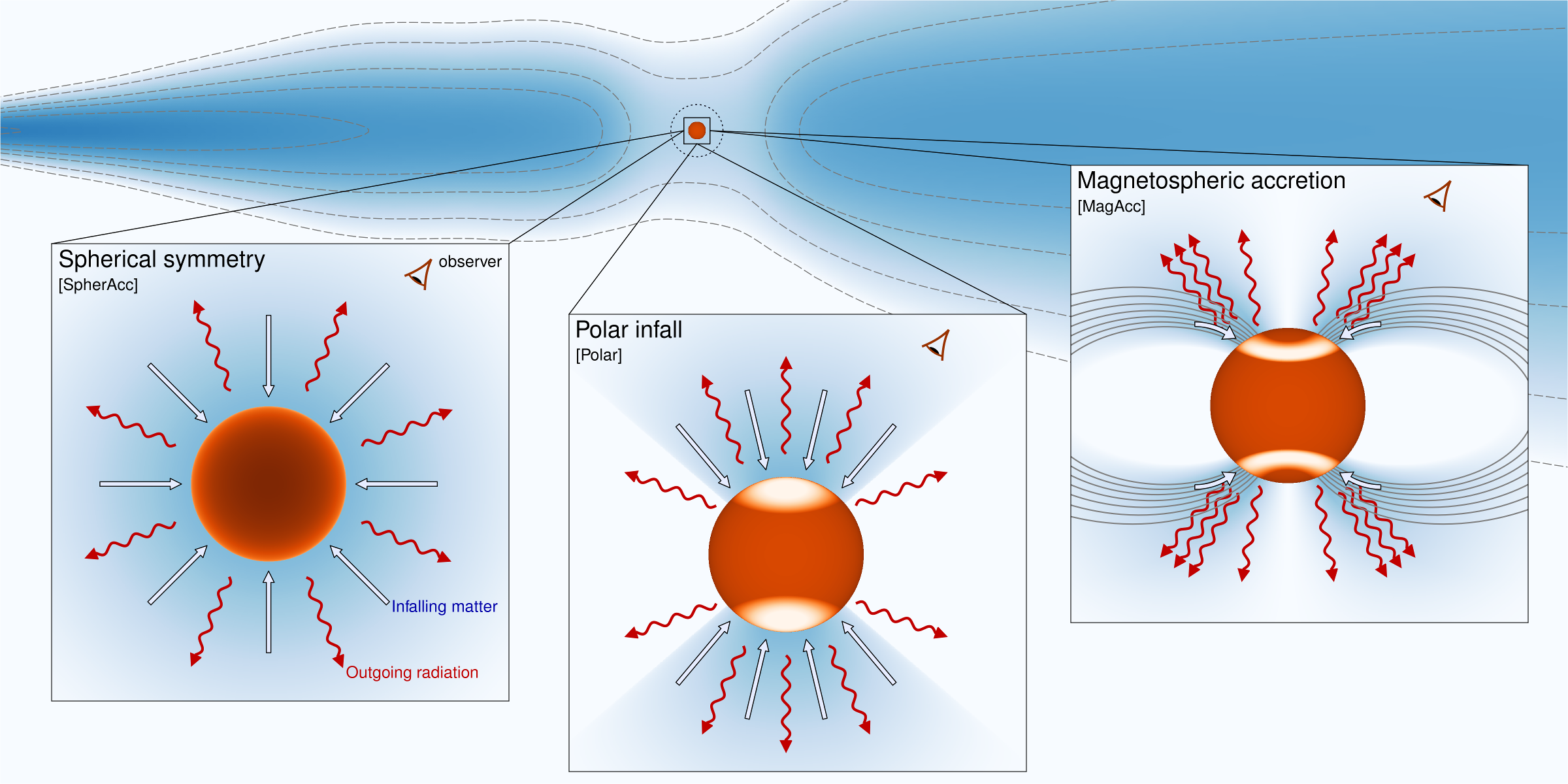
Figure 1: Schematic view of the accretion scenarios considered in this work. In spherical symmetry (SpherAcc), the gas (straight thick lines) is assumed to be distributed uniformly on the surface of the planet ($f_{\mathrm{fill}}=100\leavevmode\nobreak\ \%$), whereas in the case of polar infall (Polar) the accreting gas is concentrated near the pole regions (assumed to be uniform within $f_{\mathrm{fill}}\approx 30\leavevmode\nobreak\ \%$, and zero outside of this). In the magnetospheric accretion case (MagAcc), the magnetic field of the protoplanet leads the gas onto a small fraction of the surface (here shown as polar-ring hot spots; $f_{\mathrm{fill}}\sim 10\leavevmode\nobreak\ \%$). See Table 1. At slightly larger scales (the insets show out to ${R_{\textnormal{acc}}}$) the gas could be coming from above, falling onto the apex of the magnetic field lines (Batygin, 2018), or from a circumplanetary disc (purposefully not shown). In all cases, the radiation (H $\alpha$-coloured squiggly lines) reaching the observer passes through the matter (gas and dust) accreting onto the planet and bears the spectral imprint of this material, which is the subject of this paper. Illustration by Th. Müller (MPIA/Haus der Astronomie).

Table 1: Accretion geometries considered in this work.

Model name	$f_{\mathrm{fill}}$	$\theta_{\mathrm{min}}$	$\theta_{\mathrm{max}}$	${R_{\textnormal{acc}}}$	${r_{\rm max}}$
Spherical accretion
SpherAcc	1.0	$0{\mbox{\textdegree}}$	$90{\mbox{\textdegree}}$	$\infty$	$100\leavevmode\nobreak\ R_{\mathrm{p}}$
Polar inflow
Polar	0.3	$0{\mbox{\textdegree}}$	$46{\mbox{\textdegree}}$	$\infty$	$100\leavevmode\nobreak\ R_{\mathrm{p}}$
Magnetospheric accretion
MagAcc	0.1	$20{\mbox{\textdegree}}$	$50{\mbox{\textdegree}}$	$5\leavevmode\nobreak\ R_{\mathrm{p}}$	$\approx\frac{1}{2}{R_{\textnormal{acc}}}$

In the polar case, the accretion is assumed to be uniform within an axisymmetric cone or ring and zero outside, with the observer looking down into this region. The accreting region is defined by

$$f_{\mathrm{fill}}=\cos\theta_{\mathrm{min}}-\cos\theta_{\mathrm{max}},$$ (1)

where $\theta_{\mathrm{min}}=0$ for the pole ($\theta_{\mathrm{min}}\neq 0$ for a ring; see e.g. Kulkarni & Romanova 2013) and $\theta_{\mathrm{max}}\leqslant 90{\mbox{\textdegree}}$ is the equivalent opening angle of the accreting region at each pole. For $f_{\mathrm{fill}}=0.3$ (e.g. 15 % of the total area at the north pole and 15 % at the south pole), the equivalent opening angle from $\theta_{\mathrm{min}}=0{\mbox{\textdegree}}$ is $\theta_{\mathrm{max}}=46{\mbox{\textdegree}}$. For a ring with $f_{\mathrm{fill}}=0.1$ starting and at $\theta_{\mathrm{min}}=20{\mbox{\textdegree}}$ (for example), $\theta_{\mathrm{max}}=50{\mbox{\textdegree}}$, while $f_{\mathrm{fill}}=0.01$ would require $\theta_{\mathrm{max}}=21.6{\mbox{\textdegree}}$, or $\theta_{\mathrm{max}}=12.9{\mbox{\textdegree}}$ if instead $\theta_{\mathrm{min}}=10{\mbox{\textdegree}}$.

In reality, there is evidence for multiple accretion components in observations, in agreement with simulations (e.g. Ingleby et al., 2013; Robinson & Espaillat, 2019; Robinson et al., 2021), but our assumption of a constant local accretion rate and an infinitely sharp transition between the accreting and the non-accreting region is a minor one. Also, given that very edge-on systems are less likely to be detected or observed, there is a relatively large probability of viewing the planet indeed within $45{\mbox{\textdegree}}$ of pole-on. Therefore, we assume that the radiation is travelling only radially (i.e. away from the planet) through the accretion region towards the observer, and neglect the possibility of scattering out of the accretion cone into the line of sight towards an observer not looking down into the accretion cone.

For the magnetospheric case, in analogy to CTTSs, we consider ${R_{\textnormal{acc}}}=5\leavevmode\nobreak\ R_{\mathrm{p}}$ (Calvet & Gullbring, 1998), but also ${R_{\textnormal{acc}}}=2\leavevmode\nobreak\ R_{\mathrm{p}}$ for comparison, as the magnetic field may be weaker, whether in total or in its dipole component. We assume that the flux coming from the postshock region (the accretion “hot spots”) passes tangentially through the accretion arc to the observer and thus travels a distance ${r_{\rm max}}\approx 1/3\times\pi{R_{\textnormal{acc}}}/2\approx{R_{\textnormal{acc}}}/2$, as illustrated in Figure 1. Therefore, curvature can be ignored at the level of our approximation, and the radiative transfer can be performed also here purely radially.

This assumption of observing along the accretion column leads to a strong estimate of the amount of absorption by the accreting gas. If the optical depth is high along the accretion column, it might be more realistic for the photons to escape preferentially at an angle from the base of the accretion footpoints (see the pole-side photons in Figure 1). In this case, they would travel relatively unimpeded towards the observer. Scattering out of the accretion arc close to the planet could also contribute to the flux, depending on the system’s inclination. Thus our approach of integrating along a segment of the flow is a simple one that should maximise potential signatures.

3.2 Parameter space

For a geometry given by $(f_{\mathrm{fill}},{R_{\textnormal{acc}}},{r_{\rm max}})$, the main quantities defining the parameter space are the mass accretion rate $\dot{M}$, the planet mass $M_{\mathrm{p}}$, and the planet radius $R_{\mathrm{p}}$. We consider a range of accretion rates $\dot{M}\approx 3\times 10^{-8}$–$3\times 10^{-4}\leavevmode\nobreak\ M_{\mathrm{J}}\,\mathrm{yr}^{-1}$. The high end of the $\dot{M}$ range is higher than usually found in planet formation models (Mordasini et al., 2012b; Tanigawa & Tanaka, 2016) but could be relevant to an accretion outburst akin to the situation of FU Orionis stars (Audard et al., 2014). With these high accretion rates, we can address whether we would indeed observe a signal in the (perhaps unlikely) event a planet were caught outbursting. This range also covers the accretion rate inferred for the PDS 70 planets (Haffert et al., 2019; Manara et al., 2019).

Concerning the mass, we focus on the gas-giant and low-mass-brown-dwarf regime with $M_{\mathrm{p}}\approx 1$–$20\leavevmode\nobreak\ M_{\mathrm{J}}$. At much higher masses, the velocity of the gas at the shock is too high for H $\alpha$ to be generated in the postshock region, and the hydrogen lines are thought to be emitted by the accreting gas (Hartmann et al., 2016; Aoyama et al., 2021).

Both to reduce the dimensionality and to provide guidance as to a possible trend, we do not keep the planet radius as a free parameter but instead adopt for definiteness the fits by Aoyama et al. (2020) of the radius as a function of accretion rate and planet mass in the population synthesis calculations of Mordasini et al. (2012b, a), for their scenarios of “cold accretion” and of “hot-accretion” (see also Mordasini et al., 2017). We call these fits respectively “Cold-population fit” and “Warm-population fit”. Towards high accretion rates and masses, the radius increases with either quantity, and the warm-population fit is larger than the cold-population fit. Typical values are $R_{\mathrm{p}}=1.5$–3 $R_{\mathrm{J}}$ and 2–4 $R_{\mathrm{J}}$, with a stronger dependence of $R_{\mathrm{p}}$ on $\dot{M}$ in the “hot” case. The “cold-” and “hot accretion” scenarios represent extreme outcomes of the accretion process in which the entire accretion energy is respectively radiated away at the shock or on the contrary brought into the planet (Marley et al., 2007; Mordasini et al., 2012b; Marleau et al., 2017, 2019). We assume that the radius depends only on the total accretion rate and the mass but not on the filling factor.

A complication is that in reality, the accretion history, not only the instantaneous values, likely sets the radius. This is suggested by the results of Berardo et al. (2017), who find that during formation, planets can have a radiative (and not convective) structure for a large fraction of their outer mass layers. Thus the results of classical convective-planet structures that let us write $R_{\mathrm{p}}=R_{\mathrm{p}}(\dot{M},M_{\mathrm{p}})$, with no time dependence, might be a simplification. However, we effectively mitigate this by considering the two different fits (“cold” and “hot”), and will find that the radius does not have a major influence in any case.

Finally, there is another, minor parameter: the interior flux from the planet, characterised by an effective temperature ${T_{\textnormal{int}}}$. We assumed somewhat arbitrarily that ${T_{\textnormal{int}}}\approx 1100$ K for all models. However, the interior flux is relevant only at the lowest accretion rates, for which there will be essentially no absorption, so that in practice it is not important.

3.3 Structure of the accretion flow

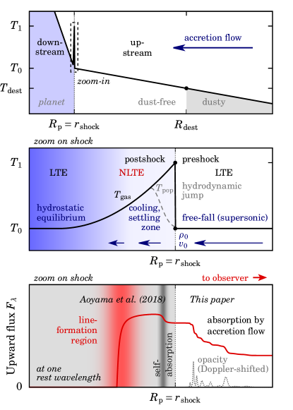
Figure 2: Overview of the structure of the accretion flow and of the shock region (see labels). Top panel: temperature (double logarithmic scale), showing the shock temperature $T_{0}$, the Zel’dovich spike up to $T\approx T_{1}$, and the dust destruction front at radius ${R_{\textnormal{dest}}}$. The shock defines the planet’s radius. The temperature flattening at $T\approx{T_{\textnormal{dest}}}$ (e.g. Marleau et al., 2019) is not shown. The next two panels focus on the dashed box. Middle panel: temperature near the shock on a linear scale. Below the hydrodynamic jump, in the NLTE cooling and settling zone, the “population temperature” of the electrons ${T_{\textnormal{pop}}}$ and the kinetic temperature ${T_{\textnormal{gas}}}$ differ at first. The temperature structure is simplified; Figure 8 of Vaytet et al. (2013b) gives a more accurate schematic. Bottom panel: upward-moving flux at one restframe wavelength within the H $\alpha$ line (red line), from the microphysical models of Aoyama et al. (2018). We illustrate the line-formation region (red) and the self-absorption (dark grey) in the settling zone, and the absorption by the accretion flow, calculated in this work. The features in the opacity (dotted grey curve; arbitrary linear scale) come from the Doppler-shift gradient (Equation (15); Figure 4).

For all accretion geometries, the supersonic infalling matter makes up the accretion flow before hitting the planet’s surface, defined as the location of the radiative hydrodynamical shock (Marleau et al., 2017, 2019). This is illustrated in Figure 2. Immediately below the hydrodynamical shock is the postshock region proper, a spatially thin “settling zone” and cooling region. There, the gas is subsonic and gradually slows down, reaching hydrostatic equilibrium at depths, where the structure is that of a non-accreting planet. The postshock region consists of the layers close to but below the shock, especially the thin cooling region. Note that an accreting planet does not have an atmosphere in the classical sense (for an isolated object), or does so at most only on the parts of its surface that are not accreting.

We now describe the mechanical and thermal structure of the accreting matter. We assume that the supersonic accretion flow is essentially spherically symmetric with purely radial motion. In general, the accretion is non-zero within a region whose boundaries in angle are set by $f_{\mathrm{fill}}$. For $f_{\mathrm{fill}}=1$ we have true spherical symmetry. Therefore, the velocity and density in the accretion flow are given by

$$v(r)= \leavevmode\nobreak\ \sqrt{2GM_{\mathrm{p}}\left(\frac{1}{r}-\frac{1}{{R_{\textnormal{acc}}}}\right)}$$ (2a)

$$= \leavevmode\nobreak\ 73\leavevmode\nobreak\ \mathrm{km}\,\mathrm{s^{-1}}\left(\frac{M_{\mathrm{p}}}{3\leavevmode\nobreak\ M_{\mathrm{J}}}\right)^{1/2}\left(\frac{r}{2\leavevmode\nobreak\ R_{\mathrm{J}}}\right)^{-1/2}\zeta^{1/2},$$ (2b)

$$\rho(r)= \leavevmode\nobreak\ \frac{\dot{M}}{4\pi r^{2}f_{\mathrm{fill}}v(r)}$$ (3a)

$$= \leavevmode\nobreak\ 3\times 10^{-12}\leavevmode\nobreak\ \mathrm{g\,cm}^{-3}\frac{1}{f_{\mathrm{fill}}}\left(\frac{\dot{M}}{\upmu M_{\mathrm{J}}\,\mathrm{yr}^{-1}}\right)$$

$$\left(\frac{M_{\mathrm{p}}}{3\leavevmode\nobreak\ M_{\mathrm{J}}}\right)^{1/2}\left(\frac{r}{2\leavevmode\nobreak\ R_{\mathrm{J}}}\right)^{-3/2}\zeta(r)^{-1/2},$$ (3b)

where

$$\zeta(r)\equiv\left(1-\frac{r}{{R_{\textnormal{acc}}}}\right),$$ (4)

with $\zeta=0.8$ for ${R_{\textnormal{acc}}}=5R_{\mathrm{p}}$ and $\zeta\rightarrow 1$ when ${R_{\textnormal{acc}}}\gg r$. For a given accretion rate, the density depends on the filling factor but the velocity does not. These are the classical formulae for an accretion flow (e.g. Calvet & Gullbring, 1998; Zhu, 2015) and have been verified to apply to planets by Marleau et al. (2017, 2019) through one-dimensional radiation-hydrodynamical simulations. For reference, the shock Mach number is in the range $\mathcal{M}\approx 10$–40 (Marleau et al., 2019), and the ram pressure of the incoming gas is given by (e.g. Berardo et al., 2017)

$$P_{\textnormal{ram}}= \leavevmode\nobreak\ \rho(R_{\mathrm{p}})v(R_{\mathrm{p}})^{2}=\frac{\dot{M}v(R_{\mathrm{p}})}{4\pi R_{\mathrm{p}}^{2}f_{\mathrm{fill}}}$$ (5a)

$$\approx \leavevmode\nobreak\ 171\leavevmode\nobreak\ \mathrm{erg\,cm}^{-3}\frac{1}{f_{\mathrm{fill}}}\left(\frac{\dot{M}}{\upmu M_{\mathrm{J}}\,\mathrm{yr}^{-1}}\right)$$

$$\left(\frac{M_{\mathrm{p}}}{3\leavevmode\nobreak\ M_{\mathrm{J}}}\right)^{1/2}\left(\frac{R_{\mathrm{p}}}{2\leavevmode\nobreak\ R_{\mathrm{J}}}\right)^{-5/2}\zeta^{1/2}.$$ (5b)

For the temperature structure of the flow, we use the results of Marleau et al. (2017, 2019). They have found that the radiative precursor (Drake, 2006; Vaytet et al., 2013b) of the shock extends to the Hill sphere (formally to infinity). This means that the infalling gas is preheated by the radiation escaping from the shock, which the work of Aoyama et al. (2018) suggests occurs mainly through the absorption of Ly $\alpha$ photons since they carry most of the shock emission flux. This contrasts to the stellar case, in which the precursor region is thin and located close to the star (see e.g. Calvet & Gullbring 1998; Colombo et al. 2019; de Sá et al. 2019) and is due to the absorption of photoionising radiation. This infinite precursor implies that the temperature profile is given by

$$T(r)=T_{0}\left(\frac{r}{R_{\mathrm{p}}}\right)^{-1/2}.$$ (6)

In turn, the equilibrium gas temperature at the shock $T_{0}$ has the value needed to radiate the mechanical energy converted to radiation as well as the interior flux:

$$acT_{0}^{4} ={F_{\textnormal{acc}}}+{\sigma}{T_{\textnormal{int}}}^{4}$$ (7a)

$$=\frac{GM_{\mathrm{p}}\dot{M}}{4\pi R_{\mathrm{p}}^{3}f_{\mathrm{fill}}}\zeta+{\sigma}{T_{\textnormal{int}}}^{4},$$ (7b)

where $v_{0}=v(R_{\mathrm{p}})$, $\rho_{0}=\rho(R_{\mathrm{p}})$, and $a$ and ${\sigma}$ are respectively the radiation and Stefan–Boltzmann constants. Marleau et al. (2017) found that the entire mechanical energy goes into radiation. Thus the radiation flux from accretion is ${F_{\textnormal{acc}}}=0.5\rho_{0}v_{0}^{3}$, leading to Equation (7b). When $\dot{M}\approx 0$, the choice of ${T_{\textnormal{int}}}\approx 1100$ K sets a minimum of $T_{0}\approx 800$ K (since $4{\sigma}=ac$; ${T_{\textnormal{int}}}$ is an effective temperature but $T_{0}$ a material temperature).

Equation (7) uses the result from Marleau et al. (2017, 2019) that the planetary accretion shock is supercritical and thus isothermal, in the sense that upstream and downstream of the Zel’dovich spike the gas temperature is set by the balance of the incoming flux of material energy and the outgoing radiative flux. This single temperature $T_{0}$ is shown in Figure 2. The shock is a “thick–thin” shock in the usual classification (e.g. Drake, 2006): the radiation is diffusive below and free-streaming above the shock. (For recent discussion of sub- and supercritical shocks, see Commerçon et al. (2011) and Vaytet et al. (2013a, b), and importantly Drake (2007) for a brief critical review of inadequate uses of these terms in the literature.) In the limit that the kinetic energy dominates over the internal flux, the shock temperature is (Marleau et al., 2019)

$$T_{0}\approx \leavevmode\nobreak\ 1280\leavevmode\nobreak\ {\rm K}\leavevmode\nobreak\ \frac{1}{f_{\mathrm{fill}}^{1/4}}\left(\frac{R_{\mathrm{p}}}{2\leavevmode\nobreak\ R_{\mathrm{J}}}\right)^{-3/4}$$

$$\times\left(\frac{\dot{M}}{\upmu M_{\mathrm{J}}\,\mathrm{yr}^{-1}}\right)^{1/4}\left(\frac{M_{\mathrm{p}}}{3\leavevmode\nobreak\ M_{\mathrm{J}}}\right)^{1/4}\zeta^{1/4}.$$ (8)

Since we focus on a line, H $\alpha$, that carries a negligible fraction of the total flux (Aoyama et al., 2018), we assume that the temperature in the accretion flow is fixed and independent of the absorption or non-absorption of the H $\alpha$ photons.

Note that Equation (6) assumes a radially constant luminosity in the accretion flow given by

$$L= \leavevmode\nobreak\ {L_{\textnormal{acc}}}+L_{\mathrm{int}}=\frac{GM_{\mathrm{p}}\dot{M}}{R_{\mathrm{p}}}\zeta+L_{\mathrm{int}},$$ (9a)

$$= \leavevmode\nobreak\ 4\times 10^{-4}\leavevmode\nobreak\ {L_{\odot}}\leavevmode\nobreak\ \left(\frac{\dot{M}}{\upmu M_{\mathrm{J}}\,\mathrm{yr}^{-1}}\right)\left(\frac{M_{\mathrm{p}}}{3\leavevmode\nobreak\ M_{\mathrm{J}}}\right)\left(\frac{R_{\mathrm{p}}}{2\leavevmode\nobreak\ R_{\mathrm{J}}}\right)^{-1}\zeta+L_{\mathrm{int}},$$ (9b)

where $L_{\mathrm{int}}=4\pi r^{2}{\sigma}{T_{\textnormal{int}}}^{4}$ is the interior luminosity from the planet. Marleau et al. (2019) showed that a constant $L(r)$ is a good approximation. However, Equation (6) does not reflect the region of a flatter, almost constant, $T(r)$ profile where the dust is destroyed, near a destruction temperature ${T_{\textnormal{dest}}}=1220\times{\rho_{-11}}^{0.0195}$ K, where $\rho_{-11}\equiv\rho\times 10^{11}\leavevmode\nobreak\ \mathrm{cm}^{3}\,\mathrm{g}^{-1}$ (Isella & Natta, 2005). In particular, Equation (6) assumes that the frequency-averaged radiation is free-streaming throughout. Thus, if the accretion flow is devoid of dust, Equation (6) will hold, while in the presence of dust this will slightly underestimate the temperature at a given radial position (and thus density). However, at these low temperatures $T\lesssim 1200$ K, the gas opacity is small anyway and we find (see Section 4) that, in the relevant part of the parameter space, the H $\alpha$ is not extincted. This justifies approximately the simplification.

We have scaled Equations (2), (3), and (3.3) using reasonable values (with $\dot{M}$ close to the minimum $\dot{M}\gtrsim 5\times 10^{-7}\leavevmode\nobreak\ M_{\mathrm{J}}\,\mathrm{yr}^{-1}$ derived by Hashimoto et al., 2020 for PDS 70 b) but one should remember that the parameter space is large, with especially $\dot{M}$, $M_{\mathrm{p}}$, and $f_{\mathrm{fill}}$ varying by orders of magnitude. Profiles in $\rho$–$T$ space are shown for a range of parameters in Figure 3. Densities are $\rho\sim 10^{-16}$–$10^{-9}$ g cm^-3 and temperatures $T\sim 100$–$10^{4}$ K, with approximately $T\propto\rho^{1/3}$, as can be seen from Equations (3) and (3.3) for $\zeta\approx 1$. An extensive discussion of the profiles, in particular against radial distance from the planet, is given in Marleau et al. (2019).

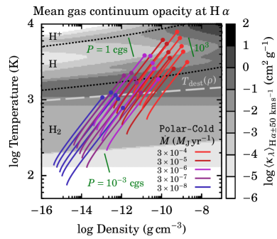
Figure 3: Structure of the accretion flow (solid lines) and gas opacity (background greyscale). The profiles are for a grid of accretion rates (isochromatic curve groups; from $\dot{M}=3\times 10^{-4}$ (top right) to $3\times 10^{-8}\leavevmode\nobreak\ M_{\mathrm{J}}\,\mathrm{yr}^{-1}$ (bottom left)) and masses ($M_{\mathrm{p}}=1$, 3, 5, 10, 20 $M_{\mathrm{J}}$ from bottom to top within each group) in the Polar-Cold case. Each profile begins on the left at ${r_{\rm max}}\approx 100R_{\mathrm{p}}$ and ends at the shock at $R_{\mathrm{p}}$ (dot), at $(\rho_{0},T_{0})$. Only the continuum opacity at H $\alpha$ (no resonance; see text) is shown averaged over $\Delta v=\pm 50\leavevmode\nobreak\ \mathrm{km}\,\mathrm{s^{-1}}$. The dust destruction line ${T_{\textnormal{dest}}}(\rho)$ is indicated (Isella & Natta, 2005; long-dashed line), and line segments show pressures $P=10^{-3}$, 1, $10^{3}$ erg cm^-3. Black dotted lines show where half of the hydrogen is molecular, atomic, or ionised. The opacity depends mostly on temperature, and most models $(\dot{M},M_{\mathrm{p}})$ include a region of high opacity, often near the shock.

3.4 Spectral profiles of shock line emission

The hydrogen line emission at the shock is taken from the models of Aoyama et al. (2020). These apply the non-LTE radiation-hydrodynamical simulations of Aoyama et al. (2018) to the shock at the surface of an accreting planet. Through detailed calculations of chemical reactions and electron transitions in hydrogen atoms, the Aoyama et al. (2018) models calculate the cooling in the disequilibrium region immediately below the hydrodynamical shock, corresponding roughly to the downstream part of the Zel’dovich spike (Vaytet et al., 2013b). See Figure 2c. This provides high-resolution profiles and line-integrated fluxes for 55 hydrogen lines in the series of Lyman, Balmer, Paschen, Brackett, etc., which are emitted from the shock towards the observer. These line profiles thus serve as the input for our calculation of the radiative transfer (Equation (14c) below), and will be seen as the black dashed lines in Figures 6–8. The line-integrated luminosity ${L_{\textnormal{H}\,\alpha}}$ as a function of $\dot{M}$ and $M_{\mathrm{p}}$ is shown in Figure 7 of Aoyama et al. (2020) and constitutes one of their main results.

The Aoyama et al. (2018) microphysical shock models depend only on the number density of hydrogen protons $n_{0}$ and the velocity $v_{0}$, both evaluated immediately before the shock. Thus $v_{0}=v(R_{\mathrm{p}})$ from Equation (2) and $n_{0}=X\rho(R_{\mathrm{p}})/m_{\mathrm{H}}$ from Equation (3), where $X$ is the hydrogen mass fraction and $m_{\mathrm{H}}$ is the hydrogen atomic mass. The number ratios are given by $\textrm{H}:\textrm{He}:\textrm{C}:\textrm{O}=1:10^{-1.07}:10^{-3.48}:10^{-3.18}$ (Cox, 2000). The present iteration of the models (Aoyama et al., 2018) covers a range $n_{0}=10^{9}$–$10^{14}$ cm^-3 and $v_{0}=20$–200 $\mathrm{km}\,\mathrm{s^{-1}}$.

With the fits of the planet radius $R_{\mathrm{p}}=R_{\mathrm{p}}(\dot{M},M_{\mathrm{p}})$ that were mentioned in Section 3.2, Equations (2) and (3) evaluated at $r=R_{\mathrm{p}}$ relate the macrophysical parameters $(\dot{M},M_{\mathrm{p}},f_{\mathrm{fill}})$ to the microphysical ones, $(n_{0},v_{0})$. For $f_{\mathrm{fill}}=1$, this leads to ranges of $n_{0}\sim 10^{10}$–$10^{14}$ cm^-3 and $v_{0}\sim 50$–200 $\mathrm{km}\,\mathrm{s^{-1}}$ for typical $(\dot{M},M_{\mathrm{p}},R_{\mathrm{p}})$ values. For small filling factors ($f_{\mathrm{fill}}\lesssim 10\leavevmode\nobreak\ \%$) or the largest accretion rates ($\dot{M}/f_{\mathrm{fill}}\gtrsim 1\times 10^{-4}\leavevmode\nobreak\ M_{\mathrm{J}}\,\mathrm{yr}^{-1}$ for the cold-population radius fit and $\dot{M}/f_{\mathrm{fill}}\gtrsim 3\times 10^{-3}\leavevmode\nobreak\ M_{\mathrm{J}}\,\mathrm{yr}^{-1}$ for $M_{\mathrm{p}}\gtrsim 10\leavevmode\nobreak\ M_{\mathrm{J}}$ in the warm-population fit), the resulting $n_{0}$ was higher than available in the previously mentioned grid and we extrapolated the spectra in preshock density. Nevertheless, this should not introduce much inaccuracy on the spectral shape or total flux.

The H $\alpha$ line is surrounded by a continuum, set by the flux from the planet’s interior. However, it is usually insignificant compared to the strong line emission. Therefore, we will neglect the continuum in the main part of this work, but do discuss this approximation in Section 4.3.3 and Appendix A.

3.5 Radiative transfer

We calculate the radiative transfer only within the accreting region, assuming spherical symmetry. For the Polar or MagAcc case, this ignores edge effects for the radiation travelling close to the walls of the accretion cone or the accretion columns, respectively; the matter and radiation properties are assumed to be independent of the angle within that region. This simplification should lead only to a modest overestimate of the amount of absorption, and is in line with other approximations in our approach.

In spherical symmetry, the radial radiative flux $F_{\lambda}$ is given in general by

$$F_{\lambda}(r)=2\pi\int_{-1}^{1}I_{\lambda}(r,\mu)\mu\,d\mu,$$ (10)

where $I_{\lambda}$ is the specific intensity in a given direction and $\mu=\cos\xi$, with $\xi$ the angle between the given direction and the radial direction. The intensity $I_{\lambda}$ is set by the radiation transfer equation, which reads (Davis et al., 2012)

$$\hat{n}\cdot\nabla I_{\lambda}(\hat{n})=\frac{dI_{\lambda}}{ds}=\alpha_{\lambda}\left(S_{\lambda}-I_{\lambda}\right),$$ (11)

where $\hat{n}$ is a unit vector defining a direction, $S_{\lambda}=j_{\lambda}/\alpha_{\lambda}$ is the source function with $j_{\lambda}$ the emissivity, $\alpha_{\lambda}$ is the coefficient of extinction including scattering and true absorption, and $s$ is the position along the ray defined by $\hat{n}$. The middle term in Equation (11) is written for the specific intensity in the direction of the ray.

We assume that the accretion flow is in local thermodynamic equilibrium (LTE), i.e. that collisions determine the electron populations in the accretion flow. Therefore, $S_{\lambda}=B_{\lambda}$ by Kirchhoff’s law, with $B_{\lambda}$ the Planck function.

In general, Equation (11) must be integrated numerically. However, the peak intensity of the H $\alpha$ line corresponds to that of a blackbody usually at a much higher temperature than the gas anywhere in the accretion flow, so that $I_{\lambda}\gg S_{\lambda}=B_{\lambda}$. Therefore, in Equation (11) the absorption term dominates over the emission, leading to

$$\frac{dI_{\lambda}}{ds}\approx-\alpha I_{\lambda}.$$ (12)

Since we are concerned with the flux at the observer (at infinity), $r\gg R_{\mathrm{p}}$ and $dI_{\lambda}/ds$ needs to be integrated only along a radial ray. This effectively neglects limb darkening. As mentioned before, we assume that the radiative quantities are independent of angle within the accretion flow. Therefore, we only need to integrate Equation (12) radially outwards from the shock at $R_{\mathrm{p}}$. The solution is $I_{\lambda}(r)=I_{\lambda}(R_{\mathrm{p}})\exp\left(-\Delta\tau_{\lambda}(r)\right)$, where

$$\Delta\tau_{\lambda}(r)\equiv\int_{R_{\mathrm{p}}}^{r}\alpha_{\lambda}(r^{\prime})\,dr^{\prime}.$$ (13)

With this, Equation (10) implies that the flux at large $r$ is

$$F_{\lambda} =2\pi\int_{-1}^{1}I_{\lambda}(R_{\mathrm{p}})e^{-\Delta\tau_{\lambda}}\mu\,d\mu$$ (14a)

$$\approx 2\pi I_{\lambda}(R_{\mathrm{p}})e^{-\Delta\tau_{\lambda}}\int_{1-0.5(R_{\mathrm{p}}/r)^{2}}^{1}\mu\,d\mu$$ (14b)

$$=F_{\lambda}(R_{\mathrm{p}})\frac{R_{\mathrm{p}}^{2}}{r^{2}}e^{-\Delta\tau_{\lambda}},$$ (14c)

taking $I_{\lambda}(R_{\mathrm{p}})$ for Equation (14b) to be constant (neglecting limb darkening) and non-zero only over the small angle $\Delta\xi\approx R_{\mathrm{p}}/r$ (around $\hat{n}$) subtended by the planet, so that also $F_{\lambda}(R_{\mathrm{p}})=\pi I_{\lambda}(R_{\mathrm{p}})$. We use Equation (14c) to calculate the flux at the observer throughout this work and do in Appendix A a comparison with the full solution to Equation (11). For most cases the approximation is excellent.

3.6 Gas opacity

The coefficient of absorption $\alpha_{\lambda}=\kappa_{\lambda}\rho$ (with dimensions of inverse length), where $\kappa_{\lambda}$ is the opacity, is divided into two contributions for the gas: the H $\alpha$ resonant (i.e. particularly strong) opacity due to the electrons in the $n=2$ quantum energy level, as well as a (pseudo-)continuum, made up of a true continuum and the superposition of many line wings. The resonant and continuum components are described in the following subsections.

The Doppler shift due to the bulk motion of the infalling gas is taken into account by evaluating for a given observer-frame (restframe) frequency $f$ the opacity at frequency

$$f^{\prime}(v)=f\left(1+\frac{v}{c}\right),$$ (15)

where $v$ is the velocity at a given position. This explains the strong variations of the monochromatic opacity shown as a grey dashed line in Figure 2c.

Given the massive uncertainties on the dust absorption, we treat it separately in Section 5. Note that for simplicity we do not include scattering as this would introduce a disproportionate level of complexity (especially for the realistic case of anisotropic scattering) compared to the rest of our approach.

3.6.1 Resonant opacity

We use standard formulae to calculate the resonant opacity (e.g. Carson, 1988; Hilborn, 2002; Sharp & Burrows, 2007; Wiese & Fuhr, 2009; Hubeny & Mihalas, 2014). Since we deal with temperatures much lower than what corresponds to H $\alpha$, we do not include stimulated emission, and approximate the ground state to be dominantly populated, which implies that the partition function is $Q(T)\approx 2$. With this approximation, we do not need to handle the well-known divergence of $Q$, which, however, can be corrected easily by the occupation probability formalism (Hubeny et al., 1994). We assume a Doppler line profile, appropriate for our temperature regime.

The strength of the resonant opacity is proportional to the number of absorbers, calculated from the Saha equation (e.g. D’Angelo & Bodenheimer, 2013). Only for the highest values of $\dot{M}/f_{\mathrm{fill}}$ and $M_{\mathrm{p}}$ is the gas at least partially ionised when reaching the shock; for most $(\dot{M},M_{\mathrm{p}})$ combinations, the hydrogen is atomic (see black dotted lines in Figure 3). At low $\dot{M}/f_{\mathrm{fill}}$ the hydrogen is molecular.

3.6.2 Continuum opacity

For the continuum gas opacity, we use very-high-resolution LTE absorption coefficients with a constant step size in wavenumber of 0.01 cm^-1, corresponding to a spectral resolution $R=1.5\times 10^{6}$. This is sufficient to resolve line cores over the relevant $(P,T)$ domain (Mollière et al., 2015, 2019). We assume a solar-metallicity (Asplund et al., 2009) mixture. The opacities of the individual species were calculated with HELIOS-K (Grimm & Heng, 2015; Grimm et al., 2021). All atoms and ions up to a proton number $Z=40$ are included, and so are the continua of H^- and collision-induced absorption (CIA) of H₂–H₂, He–H, and H₂—He. Molecular absorption is included for H₂O , CO, TiO, SH, and VO. Abundances were determined by chemical equilibrium calculations for the gas phase as provided by FastChem (Stock et al., 2018). Where needed, we extrapolate the fit of the equilibrium constants beyond their tabulated range of $T=100$–6000 K to calculate opacities from $T=100$ to $10^{4}$ K. A detailed description of chemical and opacity data for the atoms and ions can be found in Hoeijmakers et al. (2019). Molecular absorption coefficients are based on the Exomol line lists where available (Polyansky et al., 2018; McKemmish et al., 2016, 2019; Gorman et al., 2019) and on HITEMP (Li et al., 2015) otherwise. The CIA data are taken from the HITRAN database (Karman et al., 2019).

Assuming solar metallicity might not be accurate because (i) important opacity sources could be locked up in large dust grains that remain in the midplane despite meridional circulation and thus do not accrete onto the planet; (ii) molecular abundances at a given position might not correspond to the chemical-equilibrium values at the local density and temperature, if the dynamical timescale is shorter than the chemical timescale (Booth & Ilee, 2019; Cridland et al., 2020); and (iii) the accretion luminosity of the planet, in particular in the UV via photochemical reactions, can also affect the chemical abundances (Rab et al., 2019). Whether any of these effects will increase or decrease the opacity cannot be said in general and is likely not robust against the details of the modelling.

The opacity tables used in this work assume that all molecules and atoms are in the gas phase even at low temperatures. Whether for equilibrium or non-equilibrium abundances, this should not be of consequence for the absorption by the gas because below $T\approx 1000$ K, the gas opacity is very low (see Figure 3). Thus we keep this simplification, keeping in mind that the exact molecular abundances are uncertain, as discussed previously.

A formal limitation is that the absorption coefficients of molecules are tabulated only up to $T\approx 3000$ K, with the value at the highest temperature used for higher temperatures. However, in practice this is not an issue because molecules are usually not important anymore at such high temperatures due to dissociation. For atoms and ions, the tables go up to $T=6100$ K. We only consider thermal broadening and the natural line widths, except for the case of the Na and K resonance line wings, where we use the pressure-broadened line profiles provided by Allard et al. (2016) and Allard et al. (2019). We note, however, that pressure broadening is not important for this study given the range of relevant pressures ($P\sim 10^{-12}$–10^-2 bar; see Figure 3, discussed below).

We will compute the monochromatic radiative transfer (Equation (14c)) and then integrate over the line width to obtain the total line extinction. However, the (flux-)averaged opacity provides an estimate of the strength of the absorption. The wavelength range is small (the width of the emerging line is of the order of 1/2000th of the wavelength, which is $\lambda_{\mathrm{H}\,\alpha}=656.464$ nm in vacuum; Wiese & Fuhr, 2009), so that it is even sufficient to compute the direct mean opacity because the Planck function does not vary much. Indeed, at $T\approx 10^{4}$ K, the highest temperatures, the Planck function changes near H $\alpha$ over a scale of $H_{B}\equiv B_{\lambda}/(dB_{\lambda}/d\lambda)\approx 260\leavevmode\nobreak\ \mathrm{nm}$, which is much larger than the line width $\Delta v/c\times\lambda_{\mathrm{H}\,\alpha}\approx 0.1$ nm for $\Delta v=50\leavevmode\nobreak\ \mathrm{km}\,\mathrm{s^{-1}}$. Even at $T\approx 10^{5}$ K, the scale would still be $H_{B}\approx 160$ nm.

Figure 3 displays the continuum gas opacity near $\lambda_{\mathrm{H}\,\alpha}$ averaged directly over $\Delta v=\pm 50\leavevmode\nobreak\ \mathrm{km}\,\mathrm{s^{-1}}$. Shown is also the $\rho$–$T$ structure of the accreting gas for SpherAcc-Cold as an example. This wavelength range covers most of the flux emerging from the shock for all models, as Figures 6–8 will show. The opacity is at most $\kappa\sim 0.1$ cm² g^-1 at H $\alpha$ (greyscale), but note that for $T\approx 800$–1200 K the wavelength dependence (not shown) is large. In Figure 3, the resonant opacity is not included because of its strong wavelength and temperature dependence; because of the Doppler shift (Equation (15)), even an average would not provide a meaningful estimate of the typical opacity at a $(\rho,T)$ position in the structure.

We can now combine these elements to calculate the line shape of accreting planets, which we do in the following sections.

4 Absorption by the gas

We have calculated the absorption of H $\alpha$ (Equation (14c)) for a grid of accretion rates $\dot{M}$ and masses $M_{\mathrm{p}}$ for the different accretion geometries discussed in Section 3.1: a spherically symmetric inflow (SpherAcc), accretion onto the polar regions (Polar), and magnetospheric accretion (MagAcc). They are illustrated in Figure 1 and summarised in Table 1. In each case we take the emerging flux from the Aoyama et al. (2018) models and integrate the extinction along a radial radiative path starting at the shock and going out to ${r_{\rm max}}$. The density and temperature are as shown in Figure 3 for one geometry.

Section 4.1 presents and discusses in detail one combination of $\dot{M}$, $M_{\mathrm{p}}$, and $R_{\mathrm{p}}$ in the Polar-Cold geometry. Then, Sections 4.2 and following present the results for the grid of models.

4.1 One example of gas absorption

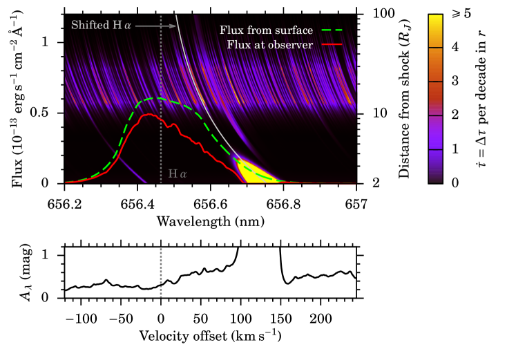
Figure 4: Top panel: H $\alpha$ line profile at spectral resolution $R=1.5\times 10^{6}$ for one case in the Polar-Cold scenario with $\dot{M}=3\times 10^{-5}\leavevmode\nobreak\ M_{\mathrm{J}}\,\mathrm{yr}^{-1}$, $M_{\mathrm{p}}=10\leavevmode\nobreak\ M_{\mathrm{J}}$, and $R_{\mathrm{p}}=2.04\leavevmode\nobreak\ R_{\mathrm{J}}$ (solid red line) when observing into the accreting area at 150 pc. The flux in the absence of absorption by the incoming matter is also shown (dashed green line). The background colour shows as a function of distance from the planet (right vertical axis) and observer-frame wavelength the strength of the absorption by the gas $\dot{\tau}(r,\lambda)$ (Equation (16)), capped at $\dot{\tau}=5$. Few regions have a higher $\dot{\tau}$, the main one being the H i resonance near the shock (reaching $\dot{\tau}\approx 5\times 10^{3}$). Indicated are also the central peak of the H $\alpha$ line in the rest frame $\lambda_{\mathrm{H}\,\alpha}$ (vertical dotted grey line) and, as a function of radial distance from the planet, the wavelength that becomes blueshifted to $\lambda_{\mathrm{H}\,\alpha}$ (see Equation (15); curved solid grey line). No dust nor ISM extinction is included. Over the brighter region at $r=15$–30 $R_{\mathrm{J}}$, the temperature is $T\approx 2000$–1500 K and the pressure $P\approx 1$–0.2 erg cm^-3 (cf. Figure 3). Bottom panel: Extinction $A_{\lambda}$ from the accretion flow against velocity offset relative to H $\alpha$.

We show the spectrally resolved line flux in Figure 4 for one case in the Polar accretion geometry, with $\dot{M}=3\times 10^{-5}\leavevmode\nobreak\ M_{\mathrm{J}}\,\mathrm{yr}^{-1}$, $M_{\mathrm{p}}=10\leavevmode\nobreak\ M_{\mathrm{J}}$, and $R_{\mathrm{p}}=2.04\leavevmode\nobreak\ R_{\mathrm{J}}$. The flux is the one seen by an observer looking into the accretion cone (within $\theta_{\mathrm{max}}=46{\mbox{\textdegree}}$ of the pole; see Figure 1) and at 150 pc, similar to the distance of well-known young star-forming regions such as Taurus, Lupus, or $\rho$ Ophiucus–Upper Scorpius. As throughout this work, no absorption by the interstellar medium (ISM) is included, to separate the two effects. Due to the absorption by the accreting gas, the line-integrated flux drops by about 32 %, corresponding to an extinction $A_{R}/\left(\mathrm{mag}\right)\approx\Delta\tau=0.4$. We now discuss the wavelength-dependent extinction.

In contrast with the line shape leaving the shock, the observable line shows small-scale structures. What dominates the absorption can be easily seen by looking at a measure of the strength of the local absorption in the flow $\dot{\tau}$, the optical depth per decade in $r$. It is given by

$$\dot{\tau}(r,\lambda)\equiv\frac{d\tau}{d\log_{10}r}=\ln(10)\,\kappa(r,\lambda)\rho(r)r.$$ (16)

This is indicated as a colourscale in Figure 4. Thus, on a logarithmic radial scale every unit $\dot{\tau}$ contributes equally to the total extinction at a given wavelength. A radial cut at one restframe wavelength is shown in Figure 2c. The obvious curvature of the opacity features is due to the Doppler shift gradient, described by Equation (15).

The quantity $\dot{\tau}$ reveals that most of the absorption occurs at $r=15$–30 $R_{\mathrm{J}}$. There, the temperatures are $T\approx 2000$–1500 K respectively (not shown), a factor $\approx 2$ lower than the shock temperature. The extinction comes mainly from the continuum opacity with a small contribution from the resonant hydrogen absorption. In general, because of the high temperatures in the postshock region (Aoyama et al., 2018), the emerging line is usually much broader than the thermal broadening of the incoming gas. Equation (15)) shows that there are only redshifted absorbers; layers moving towards the planets absorb photons blueshifted to H $\alpha$ in the frame of the accreting gas (see the curved grey line in Figure 4). Therefore, resonant absorption (by the incoming $n=2$ electrons) can occur only redward of the rest central wavelength, approximately equal to the centre of the line emerging from the postshock region. This is the yellow region in Figure 4.

Because the velocity decreases away from the planet, there is the possibility that the complete red wing be absorbed by the incoming $n=2$ electrons. However, the temperature and thus the number fraction of absorbers decrease outwards much faster than the Doppler shift. Therefore, only a small wavelength range can be absorbed by the incoming $n=2$ electrons.Also, as we calculate in Appendix A, the emission by the accretion gas in that wavelength range would be important, so that in reality the increase in the extinction would be smaller than what Figure 4b suggests (see Figure 12a).

Figure 4 shows that the Doppler shift gradient smears the strong wavelength dependence of $\dot{\tau}(r,\lambda)$ for the integrated extinction and that the resulting absorption (bottom panel) has less structure. However, in this example, there happens to be a clear downward slope in the extinction from 656.45 to 656.55 nm ($\Delta v\approx 0$–$100\leavevmode\nobreak\ \mathrm{km}\,\mathrm{s^{-1}}$), which exacerbates the asymmetry in the input line profile. The result is a crudely gaussian-looking blue wing but a linearly decreasing red wing. This leads to an apparent offset in the line peak but only by 25 $\mathrm{km}\,\mathrm{s^{-1}}$, much less than the line width.

Our temperature structure is based on frequency-integrated equations and supported by the grey flux-limited diffusion (FLD) simulations of Marleau et al. (2017, 2019). FLD is an approximate method (e.g. Ensman, 1994; Turner & Stone, 2001), but the temperature structure should be robust because it reflects global energy conservation. In particular, in our case the temperature must drop from a value of order $\approx T_{0}$ (Equation (7)) to a much lower value in the CSD and therefore cross at some point this range $T\approx 2000$–1500 K where the opacity is particularly strong. It depends on the density only weakly (see Figure 3), and for a given temperature profile $T(r)$ and thus opacity profile $\kappa(r)$, $\dot{\tau}$ goes as $\rho r\propto r^{-1/2}$ (in the limit $\zeta=1$; Equations (3) and (16)), which is not a strong dependence. Thus if the temperature of maximum absorption were at another distance from the planet, the integrated absorption should be similar. The frequency dependence would be different (because of the radial dependence of the velocity) but only quantitatively. Within the other assumptions, these results are somewhat robust since the maximum absorption does not occur in the outermost parts of the flow, where the accretion geometry is much more uncertain.

We have not considered absorption by the dust here. Taking the approximate expression for $\rho$ valid in the limit ${R_{\textnormal{acc}}}=\infty$, Equation (3) with $\zeta=1$, the gas column density is

$$\Sigma=\int_{R_{\mathrm{p}}}^{r_{\rm max}}\rho\,dr\approx\frac{\dot{M}}{2\pi f_{\mathrm{fill}}\sqrt{2GM_{\mathrm{p}}R_{\mathrm{p}}}}$$ (17)

since ${r_{\rm max}}\gg R_{\mathrm{p}}$, which yields $\Sigma=5$ g cm^-2 for this example. Thus, the dust will not be able to absorb much radiation if the dust opacity (cross-section per gram of gas, not of dust) $\kappa_{\mathrm{dust,\,H}\,\alpha}\equiv f_{\textrm{d/g}}\kappa_{\bullet,\,\mathrm{H}\,\alpha}\ll 1/\Sigma\approx 0.2$ cm² g^-1, where $\kappa_{\bullet,\,\mathrm{H}\,\alpha}$ is the dust material opacity (cross-section per gram of dust) at H $\alpha$. Comparing to the opacity values of Woitke et al. (2016), who study the effect of the variation of several relevant opacity parameters, this situation seems possible. However, the parameter space is large and the opacity itself is very uncertain. We explore the absorption by the dust in more detail and systematically in Section 5.

In the following subsections, we discuss the results from the grid of models covering the relevant planet-formation parameter space (see Section 3.2), as discussed at the beginning of this section.

4.2 Line-integrated fluxes

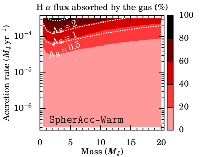
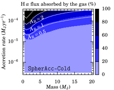
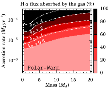
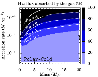
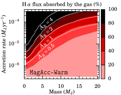
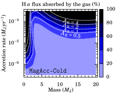
Figure 5: Percent reduction in the line-integrated flux for the SpherAcc, Polar, and MagAcc accretion geometries (top to bottom rows) from the gas opacity only. Shown are the results for the warm- (left column) and cold-population radii (right column). The dotted lines highlight an extinction $A_{R}=0.5$, 1, 2, and 4 mag (bottom to top). At a given accretion rate, high-mass planets suffer less from absorption. For moderate $\dot{M}\lesssim 10^{-5}\leavevmode\nobreak\ M_{\mathrm{J}}\,\mathrm{yr}^{-1}$, the extinction is at most $A_{R}\approx 0.5$ mag. For SpherAcc and Polar, both radius fits yield similar results.

The first two rows of Figure 5 display the relative drop in the flux $\Delta F$ across the accretion flow for the SpherAcc and Polar geometries. The drop is mainly an increasing function of $\dot{M}/f_{\mathrm{fill}}$ and ranges between $\Delta F=0\leavevmode\nobreak\ \%$ (no absorption) and nearly $\Delta F=100$ % over the parameter space considered. Already for $\dot{M}\approx 3\times 10^{-5}\leavevmode\nobreak\ M_{\mathrm{J}}\,\mathrm{yr}^{-1}$, there is noticeable absorption with $\Delta F\approx 20$–50 % depending on the mass, with more absorption at lower planet masses. This corresponds to an extinction $A_{R}\approx 2$–4 mag. The increase of extinction with decreasing planet mass (and thus, at a given $\dot{M}$, with the gas column density) can be seen from Equation (17). Also, for the three highest $\dot{M}$ values in Figure 3, the opacity increases with decreasing temperature (due to the contribution from water; Marleau et al., 2017) and increasing density, that is, decreasing mass. For moderate $\dot{M}\lesssim 10^{-5}\leavevmode\nobreak\ M_{\mathrm{J}}\,\mathrm{yr}^{-1}$, the extinction is at most $A_{R}\approx 0.5$ mag.

Interestingly, the dependence of $\Delta F$ on the mass becomes larger towards smaller filling factors. The choice of warm- or cold-population radii barely changes the outcome but the trend is as expected: $\Delta F$ is larger for the cold-population radii since they are smaller, leading to higher preshock temperatures and densities ($\tau\propto\rho$), with the temperature peaking at a few thousand kelvin (see Figure 3).

The MagAcc scenario, shown in the third row, leads to qualitatively similar but quantitatively different results. The minimum accretion rate needed to have significant absorption ($A_{R}\gtrsim 1$ mag) can be as low as $\dot{M}\sim 3\times 10^{-6}\leavevmode\nobreak\ M_{\mathrm{J}}\,\mathrm{yr}^{-1}$, at low masses $M_{\mathrm{p}}\approx 1$–5 $M_{\mathrm{J}}$. The mass dependence of $\Delta F$ is stronger for the warm-population radii, and for the cold-population radii $\Delta F$ shows clear non-monotonic behaviour. In particular, there is a “window” near $M_{\mathrm{p}}=3$–7 $M_{\mathrm{J}}$ in which the absorption corresponds only to $A_{R}\lesssim 0.5$ mag even for a colossal accretion rate $\dot{M}=10^{-4}\leavevmode\nobreak\ M_{\mathrm{J}}\,\mathrm{yr}^{-1}$; for only slightly smaller masses of $M_{\mathrm{p}}\approx 1$–2 $M_{\mathrm{J}}$, the extinction is $A_{R}\gg 4$ mag. Thus these $M_{\mathrm{p}}\approx 5\leavevmode\nobreak\ M_{\mathrm{J}}$ planets could be particularly observable. However, this depends on the viewing geometry.

Overall, these results show that absorption can be significant (several magnitudes of extinction) at higher accretion rates or for low-mass planets in the MagAcc case, particularly for smaller (cold-population) radii. However, the extinction from the gas is negligible if $\dot{M}\lesssim 3\times 10^{-6}\leavevmode\nobreak\ M_{\mathrm{J}}\,\mathrm{yr}^{-1}$.

The outer integration limit for the absorption calculation (i.e. in Equation (14c)), ${r_{\rm max}}$, is a poorly known quantity. However, one can argue that this is of little consequence: Figure 4 suggests that most of the absorption, if there is any, occurs at tens, not hundreds of Jupiter radii. This is corroborated heuristically by Figure 3, which shows that profiles with $\dot{M}\gtrsim 3\times 10^{-6}\leavevmode\nobreak\ M_{\mathrm{J}}\,\mathrm{yr}^{-1}$ cross the high-opacity region near the shock in density space, and thus also in radial distance from the planet since $\rho$ is a monotonic function of radius for $r\ll{R_{\textnormal{acc}}}$ (Equation (3)).

4.3 Line profiles

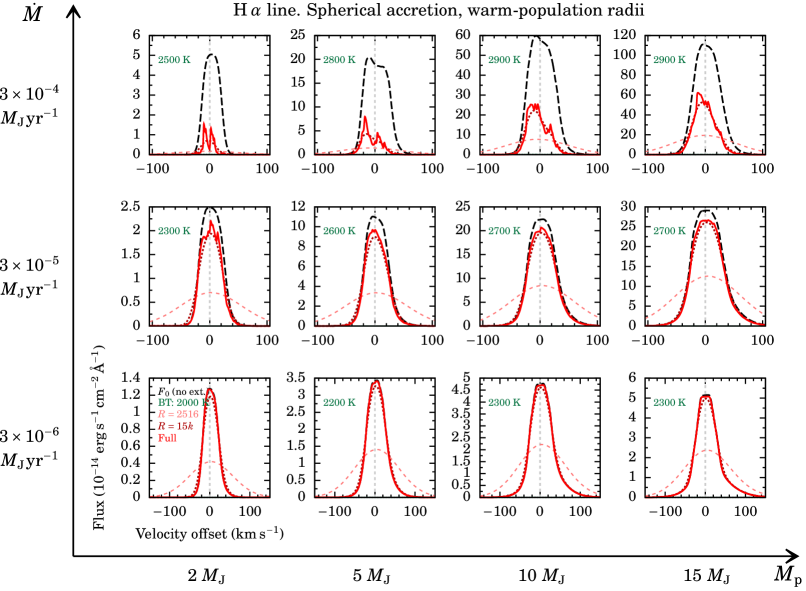
Figure 6: Effect of the extinction by the accreting gas on the H $\alpha$ profile. Shown is the flux for sources at 150 pc as a function of planet mass and accretion rate (outer axes) for the SpherAcc-Warm case of Table 1. For each subpanel, we plot the profile without extinction (black dashed line) and the profile after passing through the accreting material (red solid line). No ISM absorption is considered. The observable profiles are also shown convolved with the resolution of MUSE ($R=2516$; dashed pale red line), and of VIS-X ($R=15,000$; dashed dark red line). The heated photosphere (BT-Settl model, with ${T_{\textnormal{eff}}}$ from the fit of Aoyama et al., 2020; green dotted line and label) is too weak to be seen in any panel. The horizontal axes are the velocity offset from the line centre. The flux and velocity ranges differ from panel to panel.

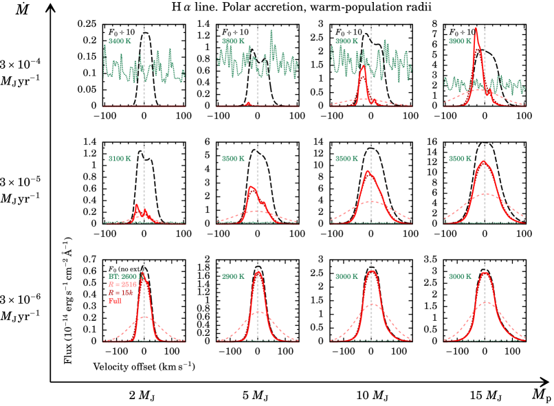
Figure 7: As in Figure 6, but for the Polar-Warm case. The observer is looking into the accreting regions, along the accretion flow. In the top row, the flux without absorption $F_{0}$ (black dashed line) has been reduced by a factor of ten to make the profiles with absorption visible.

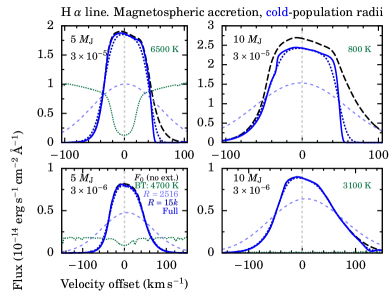
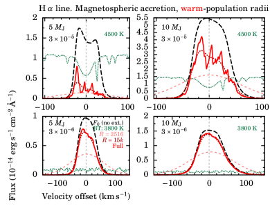
Figure 8: As in Figure 6, but for the MagAcc cases (cold and warm; left and right groups, respectively). The mass in $M_{\mathrm{J}}$ and accretion rate in $M_{\mathrm{J}}\,\mathrm{yr}^{-1}$ are indicated in each subpanel. The spectra are for an observer looking into the accretion flow towards the base of the shock or more generally for radiation passing through only the layers closest to the planet and escaping (see Figure 1). Possible rotation and inclination (between the observer and the accretion column) are not taken into account. The strong photospheric absorption (green) in some cases may not be realistic; see text.

4.3.1 Spherical and polar cases

High-resolution ($R=1.5\times 10^{6}$) line profiles are shown in Figures 6 and 7 for several cases from Figure 5 for the SpherAcc and Polar cases. The absolute spectral densities are for sources at 150 pc (relevant e.g. for Taurus, Lupus, or $\rho$ Oph–U Sco) and are mostly of order $F_{\lambda}\sim 10^{-14}$–$10^{-13}$ erg s^-1 cm^-2 Å^-1 for the range of $\dot{M}$ and $M_{\mathrm{p}}$ shown. We also show an estimate of the photospheric emission from the fit of Aoyama et al. (2020), to which we return in Section 4.3.3.

For a given $(\dot{M},M_{\mathrm{p}})$ and therefore, by assumption, radius, the line-integrated flux at the observer decreases when going from SpherAcc to Polar, that is, when reducing $f_{\mathrm{fill}}$. This is due to the increased preshock density ($n_{0}\propto\rho\propto\dot{M}/f_{\mathrm{fill}}$), which leads to more self-absorption in the postshock region (Aoyama et al., 2020; sketched in Figure 2c), thereby reducing the luminosity in the H $\alpha$ line.

As discussed in Aoyama & Ikoma (2019), the line widths (at 10 and 50 % of the maximum) of the profiles in Figures 6 and 7 reflect both the temperature of the region at which most of the line is formed as well as the absorption by the layers above this in the postshock region. We can now extend this statement by noting that the accretion flow too can change the width of the line, for $\dot{M}>3\times 10^{-5}$ ($3\times 10^{-3}$) $M_{\mathrm{J}}\,\mathrm{yr}^{-1}$ in the SpherAcc (Polar) case.

The profiles as they emerge from the accretion flow reveal further information. They exhibit, in part as expected from Figure 5, a range of qualitative outcomes: no absorption (low $\dot{M}$), moderate wavelength-independent (high $\dot{M}$ and intermediate $M_{\mathrm{p}}$), moderate wavelength-dependent absorption (intermediate $\dot{M}$ and low $M_{\mathrm{p}}$), and very strong absorption (high $\dot{M}$ and low $M_{\mathrm{p}}$). Also, different line shapes are visible: roughly Gaussian (towards the bottom right); flattened (middle right); or with self-absorption in the peak taking place in the postshock region (top and middle left).

In Figures 6 and 7, the lines at (somewhat) high accretion rates $\dot{M}\gtrsim 3\times 10^{-5}\leavevmode\nobreak\ M_{\mathrm{J}}\,\mathrm{yr}^{-1}$ display some asymmetry, as in the example shown in Figure 4. In all examples considered, an asymmetry, if present, is characterised by a peak shifted blueward by around 10 to $20\leavevmode\nobreak\ \mathrm{km}\,\mathrm{s^{-1}}$, which results from stronger absorption in the red wing. This asymmetry is present in the opacity and comes at least in part from a slight slope in the continuum of the opacity, as can be seen in Figure 4. In that example, there happen to be several stronger features in the opacity between $\Delta v\approx-10$ and $+150\leavevmode\nobreak\ \mathrm{km}\,\mathrm{s^{-1}}$ relative to the line centre. These features are physically unrelated to the H $\alpha$ line and might not be present for other elemental mixtures or atomic and molecular abundances (for instance due to disequilibrium chemistry). The asymmetry already present in the input profile grows towards lower masses. Only in a few cases is there a small dip at the central position of H $\alpha$, but this is not due to resonant absorption because the latter is redshifted as discussed in Section 4.1. For the highest accretion rates, especially at $M_{\mathrm{p}}\lesssim 5\leavevmode\nobreak\ M_{\mathrm{J}}$, the signal is reduced by orders of magnitude. This implies that a planet accreting at such high rates would be indistinguishable from the continuum, especially taking the emission from the accreting gas into account (see Figure 12b).

For the cold-population radii, the results (shown in Figures 14 and 15) are similar, with a moderate amount of extinction imprinting spectral structure at high accretion rates $\dot{M}\gtrsim 3\times 10^{-5}\leavevmode\nobreak\ M_{\mathrm{J}}\,\mathrm{yr}^{-1}$. However, the line fluxes (at the observer’s position) are either very similar or smaller, with very few exceptions. In the Cold cases, the smaller radius leads to a higher accretion luminosity (${L_{\textnormal{acc}}}\propto 1/R_{\mathrm{p}}$), but in the Warm cases the conversion of ${L_{\textnormal{acc}}}$ to ${L_{\textnormal{H}\,\alpha}}$ turns out to be more efficient by a factor greater than the ratio of the radii. Thus, overall, the flux is usually smaller in the Cold cases.

4.3.2 Magnetospheric accretion

Spectra for the MagAcc case are shown in Figure 8. In this geometry, we have assumed that the flux from the postshock region passes through the accretion column out to a distance ${r_{\rm max}}\approx{R_{\textnormal{acc}}}/2$ (i.e. tangentially through the accretion arc; see Figure 1). The high spectral resolution $R\sim 10^{6}$ of our calculations reveals pronounced features for the warm-population radii that are absent for the cold-population radii. This is due to the different highest temperatures in the flow (Equations (6 and (7)). Indeed, the shock temperature (where the maximum is reached) is $T_{0}\approx 2000$–3000 K for the warm-population case as opposed to $T_{0}\approx 4000$–7000 K for the cold case, due to the smaller radii in the latter case. For these higher temperatures in the cold-population case, close to the planet molecules are absent and only a few atomic lines and the continuum leave a spectral imprint.

There are two consequences of the short integration length. One is that the temperature does not drop into a region where molecules are important. The second consequence is that the features are sharper because they are not blurred by a gradient in the Doppler shift; in other words, over the region of the strongest absorption, roughly $R_{\mathrm{p}}$ to ${r_{\rm max}}\approx{R_{\textnormal{acc}}}/2=2.5R_{\mathrm{p}}$, the change in the Doppler shift $\Delta(\Delta\lambda)\approx dv/dr\times({r_{\rm max}}-R_{\mathrm{p}})\times\lambda_{0}/c\sim(3/4)(v_{0}/c)\lambda_{0}$ is smaller than the typical spacing between the spectral features. Finally, in a few of the examples selected (e.g. cold-population radii, $\dot{M}=3\times 10^{-5}\leavevmode\nobreak\ M_{\mathrm{J}}\,\mathrm{yr}^{-1}$, $M_{\mathrm{p}}=10$ and $5\leavevmode\nobreak\ M_{\mathrm{J}}$, $f_{\mathrm{fill}}=10\leavevmode\nobreak\ \%$), the spectral footprint of the H $\alpha$ resonance is clearly visible at $\Delta v\gtrsim+60\leavevmode\nobreak\ \mathrm{km}\,\mathrm{s^{-1}}$ as a strong absorption.

More generally, how smooth or ragged the line profile is, is determined by how large the Doppler shift gradient in the flow (not the Doppler shift itself) is over the length over which there are stronger spectral signatures, which in turn is set by the temperature structure in the flow. Very roughly speaking, the opacity is low both for $T\lesssim 800$ K and at $T\approx 3000$–6000 K (see Figure 3) and does not depend strongly on density. If the maximal temperature in the flow (at the shock) is above or close to the upper edge of the opacity maximum, a sufficiently large fraction of the flow will be in the high-opacity regime. This matters especially because both the density (thus the optical depth) and the velocity gradient are stronger closer to the shock. A maximum temperature near the opacity maximum therefore leads to a blurring of the features by the Doppler shift (i.e. velocity) gradient.

4.3.3 Importance of the continuum

So far, we have effectively considered continuum-subtracted emission lines by calculating the radiative transfer only for the shock excess. However, currently used high-resolution spectral differential imaging (HRSDI) techniques involve the subtraction of the continuum and of low-frequency spectral components (in H $\alpha$: Haffert et al., 2019; Xie et al., 2020; in the NIR: Snellen et al., 2014; Hoeijmakers et al., 2018; Petrus et al., 2021; Cugno et al., 2021). Therefore, we need to ensure that subtracting the photosphere, especially if it is somewhat mismatched, will still leave the line emission detectable. For spectrally resolved observations, what matters here is, to first order, not the ratio of the line peak to the continuum, but rather its ratio to the spread of the local (pseudo)continuum features, the “photospheric noise”.

To assess whether the photospheric emission could hinder the line measurement, we plot in Figures 6–8 the approximate photospheric emission of the planet. This is to be compared to the line emission at the planet’s surface. The more complete approach would require inputting the line together with the continuum to the radiative transfer including emission from the accretion flow (Appendix A), but for our purposes the current estimate should suffice.

We use the fit of Aoyama et al. (2020) of ${T_{\textnormal{eff}}}(\dot{M},M_{\mathrm{p}})$. These fits consider the downward-travelling radiative fluxes from the detailed shock models and ensure that the total emitted luminosity from the planet is equal to the sum of the interior and the incoming kinetic energy. Thus, for the photosphere, $\sigma{T_{\textnormal{eff}}}^{4}$ is not simply given by ${L_{\textnormal{acc}}}/(4\pi R_{\mathrm{p}}^{2}f_{\mathrm{fill}})$ because a part of this accretion energy is already emitted in the hydrogen lines and continua. Rather, the luminosity from the photosphere at ${T_{\textnormal{eff}}}$ is $L_{\mathrm{phot}}={L_{\textnormal{acc}}}+L_{\mathrm{int}}-L_{\mathrm{shock}}$, where $L_{\mathrm{shock}}$ is the total outward travelling luminosity from the shock models. This holds for the accreting region of fractional area $f_{\mathrm{fill}}$, while the rest of the planet surface has ${T_{\textnormal{eff}}}={T_{\textnormal{int}}}$.

For the spectrum, we use the high-resolution (at H $\alpha$: $\Delta\lambda=0.01$–0.05 Å, i.e. $R\approx 130,000$–$660,000$) solar-metallicity BT-Settl/AGSS2009 models (Allard et al., 2012) obtained from the SVO Theory Server and round $\log g$ to the nearest 0.5 dex and ${T_{\textnormal{eff}}}$ up (to be conservative) to the nearest multiple of 100 K. To plot against the Doppler distance $\Delta v$ from the line centre, we use as the central wavelength of the photospheric models $\lambda_{\mathrm{H}\,\alpha}=656.283$ nm in air (for the BT-Settl models on the SVO server; Wiese & Fuhr, 2009).

For the SpherAcc-Warm case (Figure 6), the continuum is never visible on the linear scale of the line peak and would need to be $\sim 10$ stronger to be even barely noticeable. Thus the photospheric emission is entirely negligible. In the Polar-Warm case (Figure 7) for $\dot{M}\lesssim 3\times 10^{-4}\leavevmode\nobreak\ M_{\mathrm{J}}\,\mathrm{yr}^{-1}$, the continuum noise is not important, but for the highest accretion rate it makes the H $\alpha$ line undetectable, except at 15 $M_{\mathrm{J}}$. In the SpherAcc-Cold and Polar-Cold cases (Figures 14 and 15), the photospheric noise is mostly very low, with some exceptions at the highest accretion rate.

In the MagAcc-Warm or -Cold cases shown in Figure 8, the photospheric noise (i.e. the amplitude of the features) is small to insignificant for most cases shown. The exception is for the combination ($M_{\mathrm{p}}=5\leavevmode\nobreak\ M_{\mathrm{J}}$, $\dot{M}=3\times 10^{-5}\leavevmode\nobreak\ M_{\mathrm{J}}\,\mathrm{yr}^{-1}$), whether in the Warm or in the Cold scenario, in which the H $\alpha$ line is in absorption in the atmospheric spectrum, with the other features smaller. This is maybe not realistic because the BT-Settl models were calculated with the pressure–temperature structure of an isolated, not accreting, atmosphere. From Equation (5a), the ram pressure for the cases in Figure 8 is $P_{\textnormal{ram}}\approx 3\times 10^{-3}$–$3\times 10^{-2}$ bar. These pressures are likely neither very far up in the atmosphere nor very deep, in which cases the shock would, respectively, not or very much change the structure. Therefore, without detailed calculations of the resulting pressure–temperature structure of the atmosphere and the radiation transport, it is difficult to estimate the effect of the heating by the shock on the line emerging from the atmosphere below the shock.

4.3.4 Observability

Line-integrated luminosities of our models are presented in Aoyama et al. (2020), and the line-integrated extinction in Section 4.2. Up to now, the few known accreting low-mass objects have been observed in H $\alpha$ filters with a width of order of 1–2 nm (Wagner et al., 2018; Zhou et al., 2021) or with MUSE at a resolution $\Delta\lambda\approx 0.3$ nm (Haffert et al., 2019; Eriksson et al., 2020). However, as seen in Section 2, much more powerful instruments are underway or expected soon. For example, with $R\geqslant 130,000$, the resolution of RISTRETTO is comparable to the effective resolution of the model curves given the native width of the spectral features and the slight smear coming from the velocity gradient. Therefore, we discuss in this section the observability at high resolution of accreting planets whose line profiles are in part shaped by the accreting gas.

In Figures 6, 7, and 8, we show line profiles $F_{\lambda}(\lambda)$ for our grid of models convolved to $R=2516$ (for MUSE and slightly broader than HARMONI) and to $R=15,000$ (for VIS-X). The full-resolution curve (for RISTRETTO) was discussed above, and Subaru+SCExAO/RHEA with $R=60,000$ is in an intermediate range. The flux densities are for an observer on Earth for a source $d=150$ pc away, typical of several star-forming regions.

The resolution of MUSE corresponds to $\Delta v=120\leavevmode\nobreak\ \mathrm{km}\,\mathrm{s^{-1}}$, which is much larger than the spectral features. Therefore, they are not recognisable at this resolution. In some cases, very slight asymmetries between the red and blue wings are visible but they would be undetectable given any amount of noise and given the finite number of pixels per resolution element. Unfortunately, the higher resolution of HARMONI with $\Delta v=100\leavevmode\nobreak\ \mathrm{km}\,\mathrm{s^{-1}}$ will not yield a significant improvement. This emphasises the need for very-high-resolution spectrographs.

Even at $R=15,000$ ($\Delta v=20\leavevmode\nobreak\ \mathrm{km}\,\mathrm{s^{-1}}$), the finest spectral features are not distinguishable. Nevertheless, some asymmetries are preserved, for instance in the Polar case at $(\dot{M}=3\times 10^{-5}\leavevmode\nobreak\ M_{\mathrm{J}}\,\mathrm{yr}^{-1},M_{\mathrm{p}}=2$–$5\leavevmode\nobreak\ M_{\mathrm{J}})$, or more clearly at the highest $\dot{M}$ and $M_{\mathrm{p}}$. This leaves the line centre shifted by approximately $-20\leavevmode\nobreak\ \mathrm{km}\,\mathrm{s^{-1}}$. Such large offsets are not expected from other effects such as planetary spin or orbital motion (see Section 7.4). Therefore, a line displaced from the theoretical value by a large amount could be a tell-tale sign of extinction from the surrounding gas.

In summary, the spectral resolving power of planned instruments such as RISTRETTO and VIS-X will make it possible in the next few years to start studying in detail the line profiles of low-mass companions, revealing the spectral imprint of the absorbing gas in the accretion flow.

5 Absorption by the dust

So far, we have neglected the contribution from the dust in our radiative transfer calculation. Since dust exists only at low temperatures and these temperatures tend to be reached at larger distances from the planet, the outer parts of the accretion flow can be important for setting the total optical depth. In the case of accretion directly onto the planet, it seems likely that the last stages, that is, close to the planet surface, are radial and supersonic. This leaves only the filling factor as the main free parameter of the accretion geometry relevant for the gas. In the case of the dust, however, the fact that parts further out can contribute makes the analysis more tentative.

Given these uncertainties, we estimate what dust opacity is needed to have a significant optical depth in the accretion flow (Section 5.1). We then derive a range of plausible values for the dust opacity based on the relevant recent literature (Section 5.2), and in Section 5.3 compare this to other recent estimates. We derive the total dust optical depth in Section 5.4.

There is only a small range of temperatures in which (i) gas–magnetic field coupling is possible thanks to sufficient ionisation ($T\gtrsim 1000$ K; Desch & Turner, 2015) and (ii) at the same time the dust has not been evaporated ($T\lesssim{T_{\textnormal{dest}}}\approx 1500$ K, ${T_{\textnormal{dest}}}$ being the temperature at which the last component of the dust evaporates; Pollack et al., 1994; Semenov et al., 2003). In other words, in the MagAcc scenario the temperature is usually too high for dust to survive. Therefore, we will put MagAcc aside for this section.

5.1 Calculating the optical depth

We first calculate the optical depth of the dust in the accretion flow. Given the large uncertainties on the dust opacity (see Section 5.2), we take a crude approach and let the dust opacity be independent of density and temperature in the region where dust is present ($T<{T_{\textnormal{dest}}}$, or $r>{R_{\textnormal{dest}}}$). The contribution of the dust to the optical depth through the accreting matter is given by

$$\tau_{\mathrm{dust,\,H}\,\alpha}=\int_{R_{\textnormal{dest}}}^{r_{\rm max}}f_{\textrm{d/g}}\kappa_{\bullet,\,\mathrm{H}\,\alpha}\,\rho\,dr,$$ (18)

where we remind that $\kappa_{\bullet,\,\mathrm{H}\,\alpha}$ is the opacity of the dust at H $\alpha$ as a cross-section per unit mass of dust. We have defined in Section 4.1 the dust opacity as a cross-section per gram of gas as $\kappa_{\mathrm{dust,\,H}\,\alpha}\equiv f_{\textrm{d/g}}\kappa_{\bullet,\,\mathrm{H}\,\alpha}$ and will use this below. The dust-to-gas mass ratio is essentially zero at $r<{R_{\textnormal{dest}}}$, which is why the lower limit of the integration is the “dust destruction front” ${R_{\textnormal{dest}}}$ (Stahler et al., 1980). From Equation (6), this is:

$${R_{\textnormal{dest}}}=\left(\frac{T_{0}}{{T_{\textnormal{dest}}}}\right)^{2}R_{\mathrm{p}}$$ (19)

if the shock temperature is larger than ${T_{\textnormal{dest}}}$. At low $\dot{M}$ there is no destruction radius in the classical sense because the dust survives down to the shock (see Figure 3 and Section 6.2 of Marleau et al. 2019). In that case the lower limit of the integral in Equation (18) is $R_{\mathrm{p}}$ instead of ${R_{\textnormal{dest}}}$. For simplicity, we do not take the weak density dependence of ${T_{\textnormal{dest}}}$ (Isella & Natta, 2005) into account. The dust destruction front is illustrated in Figure 2.

Since $\rho\propto r^{-3/2}$ (Equation (3b) when $\zeta=1$), the integral in Equation (18) will converge, as ${r_{\rm max}}$ tends to infinity, if $\kappa_{\mathrm{dust,\,H}\,\alpha}$ is constant or does not increase faster than $r^{1/2}$. However, this also assumes that the accretion radius ${R_{\textnormal{acc}}}$ is sufficiently large; if not, the outer parts of the flow contribute significantly because the density $\rho\propto v$ is higher there due to the smaller velocity $v\propto(1/r-1/{R_{\textnormal{acc}}})$.

If ${R_{\textnormal{dest}}}\geqslant R_{\mathrm{p}}$ and in the limit ${r_{\rm max}}\gg{R_{\textnormal{dest}}}$ and ${R_{\textnormal{acc}}}\gg R_{\mathrm{p}}$, the optical depth (Equation (18)) becomes

$$\tau_{\mathrm{dust,\,H}\,\alpha}= \leavevmode\nobreak\ f_{\textrm{d/g}}\kappa_{\bullet,\,\mathrm{H}\,\alpha}{T_{\textnormal{dest}}}\left(\frac{{\sigma}\dot{M}^{3}R_{\mathrm{p}}}{4\pi^{3}f_{\mathrm{fill}}^{3}G^{3}M_{\mathrm{p}}^{3}}\right)^{1/4}$$ (20a)

$$= \leavevmode\nobreak\ 0.2\,\left(\frac{f_{\textrm{d/g}}}{10^{-4}}\right)\left(\frac{\kappa_{\bullet,\,\mathrm{H}\,\alpha}}{10^{4}\leavevmode\nobreak\ \mathrm{cm}^{2}\,\mathrm{g}_{\mathrm{dust}}^{-1}}\right)\left(\frac{{T_{\textnormal{dest}}}}{1500\leavevmode\nobreak\ \mathrm{K}}\right)$$

$$\times\left(\frac{f_{\mathrm{fill}}}{0.30}\right)^{-3/4}\left(\frac{\dot{M}}{\upmu M_{\mathrm{J}}\,\mathrm{yr}^{-1}}\right)^{3/4}\left(\frac{M_{\mathrm{p}}}{5\leavevmode\nobreak\ M_{\mathrm{J}}}\right)^{-3/4}$$

$$\times\left(\frac{R_{\mathrm{p}}}{2\leavevmode\nobreak\ R_{\mathrm{J}}}\right)^{1/4},$$ (20b)

where the subscript “dust” in the units of $\kappa_{\bullet,\,\mathrm{H}\,\alpha}$ indicates that this is the cross-section per gram of dust, that is, the intrinsic (material) cross-section. Equation (20b) was written with $R_{\mathrm{p}}$ as an independent quantity while in our fits it depends on $\dot{M}$ and $M_{\mathrm{p}}$. However, $\tau_{\mathrm{dust,\,H}\,\alpha}$ does not depend strongly on $R_{\mathrm{p}}$ (only as the fourth root). The $f_{\mathrm{fill}}$ factor on the denominator in these expressions comes from the fact that $\tau_{\mathrm{dust,\,H}\,\alpha}$ is the optical depth through the accretion flow, with $\rho\propto\dot{M}/f_{\mathrm{fill}}$ (see Equation (3)). Thus the optical depth should increase with increasing accretion rate (all the more since $R_{\mathrm{p}}$ also grows with $\dot{M}$), whereas it should decrease somewhat with mass (in part counterbalanced by the growth of $R_{\mathrm{p}}$ with $M_{\mathrm{p}}$, but only weakly because $\tau_{\mathrm{dust,\,H}\,\alpha}\propto R_{\mathrm{p}}^{1/4}$). Unfortunately, $\tau_{\mathrm{dust,\,H}\,\alpha}$ has a non-negligible dependence (linear) on the very uncertain quantities $f_{\textrm{d/g}}$ and $\kappa_{\bullet,\,\mathrm{H}\,\alpha}$. In this light, the uncertainty on ${T_{\textnormal{dest}}}$ and its weak density dependence do not matter.

The prefactor in Equation (20b) implies that for the nominal values in that equation, the dust is not able to absorb much H $\alpha$ emission, with a flux decrease $\Delta F=1-\exp(-0.2)\approx 20$ %. The parameter space is large, however, and we explore it more systematically in this and the following sections.

One can ask what the minimum average dust opacity (as a cross-section per unit mass of gas) is needed to have $\tau_{\mathrm{dust,\,H}\,\alpha}\sim 1$. Equation (18) can be written as

$$\tau_{\mathrm{dust,\,H}\,\alpha}=\tilde{\Sigma}_{\textrm{gas}}\langle\kappa_{\mathrm{dust,\,H}\,\alpha}\rangle,$$ (21)

where

$$\tilde{\Sigma}_{\textrm{gas}}\equiv\int_{R_{\textnormal{dest}}}^{r_{\rm max}}\rho\,dr$$ (22)

is the gas column density of the accretion flow where the dust is present (as opposed to the full column density) and $\langle\kappa_{\mathrm{dust,\,H}\,\alpha}\rangle=\langle f_{\textrm{d/g}}\kappa_{\bullet,\,\mathrm{H}\,\alpha}\rangle$ is the dust absorption cross-section per unit gas mass averaged over that part of the accretion flow. Since we assumed the dust material opacity to be constant where it is non-zero, and if we also take $f_{\textrm{d/g}}$ constant in the accretion flow, it holds simply that $\langle\kappa_{\mathrm{dust,\,H}\,\alpha}\rangle=\kappa_{\mathrm{dust,\,H}\,\alpha}$. Equation (21) implies that $\tilde{\Sigma}_{\textrm{gas}}^{-1}$ is equal to the minimum dust opacity (as a cross-section per unit mass of gas) needed to have $\tau_{\mathrm{dust,\,H}\,\alpha}\approx 1$ and thus contribute noticeably to the absorption. Over the narrow width of the line ($\Delta\lambda\lesssim 0.001\leavevmode\nobreak\ \upmu$m), the dust opacity is constant, so that it can affect only the total flux but not the line shape.

Figure 9a displays the minimum average dust opacity required to have an optical depth of unity. We focus on the SpherAcc and Polar cases. We find that over the parameter range considered but restricting ourselves to $\dot{M}\lesssim 3\times 10^{-5}\leavevmode\nobreak\ M_{\mathrm{J}}\,\mathrm{yr}^{-1}$, the minimum dust opacity required in order for the dust to absorb a significant fraction of the H $\alpha$ signal is of order $\tilde{\Sigma}_{\textrm{gas}}^{-1}\gtrsim 1$–100 cm² g^-1. The results of Figure 9a are only moderately sensitive to the planet mass and scale roughly as $\Sigma_{\mathrm{dust}}\sim\dot{M}^{1.5}$. The choice of the cold- or warm-population radii is not crucial (not shown), and the filling factor only has a moderate effect (solid vs. dashed lines). For most of parameter space, the shock is hot enough that the dust destruction radius is at several times the planet radius, which typically corresponds to ${R_{\textnormal{dest}}}\approx 10$–30 $R_{\mathrm{J}}$ (see grey dotted lines). For increasing accretion rate, the size of the dust-free inner region relative to the planet radius, ${R_{\textnormal{dest}}}/R_{\mathrm{p}}$, grows. Nevertheless, the dust column density increases with $\dot{M}^{1.5}$, so that the minimum opacity required becomes smaller.

We have assumed that the dust opacity has a constant value throughout the accretion flow at $r>{R_{\textnormal{dest}}}$ and is zero within the dust destruction front. If it is not too far out (i.e. if ${R_{\textnormal{dest}}}\ll{r_{\rm max}}$), and assuming that ${R_{\textnormal{acc}}}\gg R_{\mathrm{p}}$, the dust optical depth $\tau_{\mathrm{dust,\,H}\,\alpha}$ can be expressed analytically (Equation (20)). In this case, but also in general, $\tau_{\mathrm{dust,\,H}\,\alpha}$ depends linearly on the dust opacity. We now turn to the task of estimating its value.

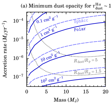
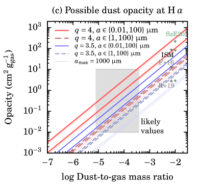
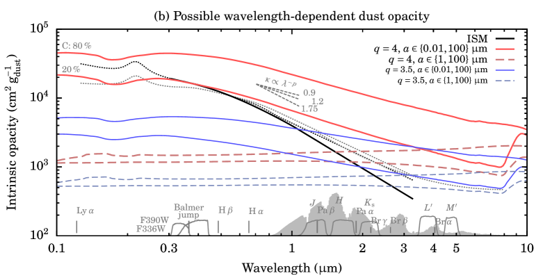
Figure 9: Estimate of the dust absorption in the accretion flow. (a) Minimum dust opacity at H $\alpha$, $f_{\textrm{d/g}}\kappa_{\bullet,\,\mathrm{H}\,\alpha}$ (per unit gas mass; contour labels), needed to have $\tau_{\mathrm{dust,\,H}\,\alpha}\approx 1$ in the accretion flow onto a growing gas giant (Equation (21)) in the Polar (solid lines) and SpherAcc (dashed lines) cases. We take the cold-population radii and fix ${T_{\textnormal{dest}}}=1500$ K. Grey dotted lines show where ${R_{\textnormal{dest}}}/R_{\mathrm{p}}=1.5$ and 5 (Equation (19)). (b) Material opacity $\kappa_{\bullet,\,\mathrm{H}\,\alpha}$. We show the ISM fits of Cardelli et al. (1989) for $R_{V}=3.1$ (dotted black) and 5.5 (dotted grey), with the absolute scale from Güver & Özel (2009); Wang & Chen (2019) (solid black); and Chiar & Tielens (2006) (dotted grey, up to 8 $\upmu$m). Red and blue curves are for size distributions set by the slope $q$ and minimum size (see legend). Curves for each model are for 20 or 80 % carbon (bottom to top), with silicate completing. At the bottom, hydrogen lines, two HST filters, and NACO IR filters are shown. The grey area is a BT-Settl model with ${T_{\textnormal{eff}}}=1200$ K and $\log g=4$. (c) Estimate of the dust opacity $\kappa_{\mathrm{dust,\,H}\,\alpha}=f_{\textrm{d/g}}\kappa_{\bullet,\,\mathrm{H}\,\alpha}$ in the accretion flow. Pale dotted lines are for $a_{\rm max}=1$ mm instead of $0.1$ mm. Red curves represent recent simulation results (see text), with a low dust abundance $f_{\textrm{d/g}}\sim 10^{-5}$–$10^{-4}$, implying $\kappa_{\mathrm{dust,\,H}\,\alpha}\sim 0.3$ cm² g^-1 with a half-spread $\sigma=1.5$ dex (grey shaded region). The opacity of Flock et al. (2016, “F+16”), Rab et al. (2019, “R+19”), and Sanchis et al. (2020, “ISM”) is shown for $f_{\textrm{d/g}}=0.01$ (grey symbols, shifted left) and the pure-graphite, “mixture”, and pure-silicate opacity of Szulágyi & Ercolano (2020, “SzE20”) is shown (green circles; top to bottom). All but Flock et al. (2016) assume $f_{\textrm{d/g}}=0.01$ in their work.

5.2 Realistic estimates of dust opacity

5.2.1 General considerations about dust parameters

The dust monochromatic opacity is set amongst others by the composition, shape, space- and time-dependent size distribution, and dynamics of dust particles in CSDs (Andrews, 2020) and specifically in the vicinity of a growing and migrating gas giant (e.g. Pollack et al., 1994). In particular, the dust-to-gas mass ratio $f_{\textrm{d/g}}$ and—to a lesser extent (Chachan et al., 2021)—the minimum and maximum grain sizes $a_{\rm min}$ and $a_{\rm max}$ impact the opacity (e.g. Cuzzi et al., 2014; Kataoka et al., 2014; Woitke et al., 2016; Krapp et al., 2021). In turn, these properties are set by many processes (e.g. Flock et al., 2016; Birnstiel et al., 2018; Vorobyov et al., 2018; Drażkowska et al., 2019; see review in the latter work).

To obtain accurate dust opacities would require global-disc radiation-hydrodynamic simulations following the dust growth, drift, and evaporation with sufficiently high resolution both in space and in the dust size, while covering the full range of grain sizes that set the opacity, and taking the feedback of the grains on the disc structure into account. This is not yet computationally feasible. However, different studies have looked at some of these aspects (e.g. Drażkowska et al., 2019; Savvidou et al., 2020; Chachan et al., 2021; Binkert et al., 2021; Szulágyi et al., 2021; Krapp et al., 2021), with some properties emerging. We highlight briefly four of them.

Firstly, since the density in the accretion flow decreases outwards, the layers in the dusty part of the flow (where $T\lesssim 1500$ K) that are closest to the planet will likely contribute the most. For $T\gtrsim 700$ K, only silicate along with carbon, iron, or troilite remain (Semenov et al., 2003; Woitke et al., 2016). Secondly, in 2D simulations, the pressure perturbation of the planet keeps the large grains outside of its orbit (“filters them out”; e.g. Paardekooper & Mellema, 2004; Rice et al., 2006; Zhu et al., 2012; Bae et al., 2019). For example, Drażkowska et al. (2019) found a maximum grain size $a_{\rm max}\sim 0.03$ cm around the planet instead of $a_{\rm max}\sim 3$ cm at larger orbital radii in theirglobal-disc hydrodynamical simulations combined with a dust evolution model. Also the size distribution near the planet is different, with $n(a)\propto a^{-q}$ with $q\approx 4$, where $n(a)$ is the number density of grains of size $a$ (J. Drażkowska 2020, priv. comm.). This is steeper than the commonly used Mathis et al. (1977) ISM distribution with $q=3.5$.

In 3D, meridional circulation could bring large grains towards a forming planet (Bi et al., 2021; Szulágyi et al., 2021), bridging the pressure bump. Realistically, this however depends on the amount of turbulence and settling (Dullemond & Dominik, 2004) and the strength, for instance, of the vertical shear instability (VSI; Flock et al., 2020), or the viscosity and the gap depth (Kanagawa et al., 2018).

Thirdly, a range of different minimum grain sizes $a_{\rm min}$ is used in the literature: $a_{\rm min}=0.1$–1 $\upmu$m (e.g. Okuzumi et al., 2012; Kataoka et al., 2014; Bae et al., 2019; Stammler et al., 2019; see brief review in Xiang et al., 2020); $a_{\rm min}=1\leavevmode\nobreak\ \upmu$m in Drażkowska et al. (2019) but with some pile-up near $a_{\rm min}$ in the resulting distribution; Flock et al. (2016) used a smaller value: $a_{\rm min}=5\leavevmode\nobreak\$nm.

Fourthly, concerning the dust abundance, the simulations of Pinilla et al. (2012) or Drażkowska et al. (2019) find depletions by a factor of $10^{3}$–$10^{4}$ relative to the global disc abundance. In a sample of seven discs, Powell et al. (2019) found with a method independent of a tracer-to-mass conversion a global dust-to-gas ratio of order $f_{\textrm{d/g}}\sim 10^{-4}$–$10^{-3}$. Recent global-disc simulations of grain growth and drift (e.g. Savvidou et al., 2020; Chachan et al., 2021) lend support to this. Finally, if planets form early (e.g. (Manara et al., 2018)), the dust particles may be locked up in macroscopic objects (pebbles, planetesimals, planetary cores), also reducing $f_{\textrm{d/g}}$.

We assume that the dust flowing onto the planet has the same size distribution as in the gap around the planet on scales of ${R_{\textnormal{Hill}}}$. Based on the previous discussion, to estimate the dust opacity we consider the following parameter values: $a_{\rm min}\in\{0.01,1\}\leavevmode\nobreak\ \upmu$m, $a_{\rm max}\in\{0.1,1\}$ mm, $q\in\{3.5,4\}$, the fraction of (amorphous) carbon $f_{\mathrm{C}}\in\{0.2,0.8\}$ by mass, with the rest made up of the usual astrophysical silicate (pyroxene: Mg_0.7Fe_0.3SiO₃), and the porosity $P\in\{0.1,0.2,0.3\}$, the vacuum fraction by volume (and not by mass).

As shown in Woitke et al. (2016), $\kappa_{\bullet,\,\mathrm{H}\,\alpha}$ increases with increasing $q$ (more small grains) and $f_{\mathrm{C}}$ (more carbon relative to silicate) or with decreasing $a_{\rm min}$ (smaller grains included) or $a_{\rm max}$ (larger grains excluded). The dependence of the opacity on the size can be understood from the fact that small grains have a larger cross-section-to-mass (area-to-volume) ratio than large grains. For the parameter values here, the opacity is almost insensitive to the porosity $P$, varying at most (at the highest carbon fraction) by 30 % for the range of $P$ covered here. Therefore, we fix $P=0.2$ hereafter.

5.2.2 Resulting monochromatic dust opacity

To calculate the dust opacity, we use with the convenient OpTool (Dominik et al., 2021), which uses Toon & Ackerman (1981) and, amongst others, the “distribution of hollow spheres” (Min et al., 2005). Optical constants are from Zubko et al. (1996) and Dorschner et al. (1995) for the carbon and silicates, respectively. Other parameters are as preset.

We plot in Figure 9b the opacity from the UV to the mid-infrared (MIR) for different dust models. We label the curves by $q$, $a_{\rm min}$, and $a_{\rm max}$. At H $\alpha$, this leads to a similar or larger range of opacities compared to including other materials such as iron (troilite) or water (ice) or even CHON organic material, and varying their abundance. Silicate-rich grains ($f_{\mathrm{C}}=0.2$) lead to strong absorption at 10 $\upmu$m (the “ten-micron bump”).

For these opacity curves, the logarithmic average opacity slope $p_{\textnormal{UV}}=\Delta\log\kappa/\Delta\log\lambda$ between H $\beta$ ($\lambda_{\mathrm{H}\,\beta}=486$ nm) and H $\alpha$ is roughly $p_{\textnormal{UV}}\approx-0.5$ to $-1$. Larger dust grain size distribution powerlaw exponent values $q$ and smaller values of $a_{\rm min}$ make the slope steeper, that is, $p_{\textnormal{UV}}$ more negative, while $a_{\rm max}$ essentially does not change the slope much (see Figure 3 of Woitke et al., 2016) and only decreases the absolute amount of extinction. For comparison, the extinction law of Cardelli et al. (1989), valid at H $\alpha$ and H $\beta$, has $p_{\textnormal{UV}}=-1.2$ ($p_{\textnormal{UV}}=-0.9$) for $R_{V}=3.1$ ($R_{V}=5$). Wang & Chen (2019) recently adjusted the Cardelli et al. (1989) extinction law with $R_{V}=3.1$ and obtained $p_{\textnormal{UV}}=-1.4$. We note that the fundamental reason why our curves are flatter than the empirical ISM curve is not yet understood.

For reference, we indicate in Figure 9b the position of some hydrogen lines and of the Balmer jump (H $\infty$ at 3646 Å) as well as the flanking $U$-band F336W and F390W filters of the Hubble Space Telescope (HST). This is motivated by the recent detection of PDS 70 b by Zhou et al. (2021) at F336W, a first for an accreting planet. We also diplay NIR and MIR filters from VLT/NACO ($J$, $H$, $K_{\mathrm{s}}$, $L^{\prime}$, $M^{\prime}$). Finally, we also show a scaled spectrum with ${T_{\textnormal{eff}}}=1200$ K and $\log g=4$ from BT-Settl, which approximately fits the data for PDS 70 b (Stolker et al., 2020a; Wang et al., 2021b).

Figure 9c displays the opacity $\kappa_{\mathrm{dust,\,H}\,\alpha}$ as a function of $f_{\textrm{d/g}}$. We consider that a range of $f_{\textrm{d/g}}\sim 10^{-5}$–$3\times 10^{-4}$ is plausible given the relative depletion by a factor of 100–1000 found by Drażkowska et al. (2019) and spatial variations (on scales larger than planets’ Hill spheres, as the results of Soon et al., 2019 suggest).

We obtain that the material opacity of the dust can be anywhere between $\kappa_{\bullet,\,\mathrm{H}\,\alpha}\sim 300$ and $3\times 10^{4}$ cm² g${}^{-1}_{\mathrm{dust}}$, which translates into $\kappa_{\mathrm{dust,\,H}\,\alpha}\sim 10^{-2}$–$10$ cm² g${}^{-1}_{\textrm{gas}}$ at $f_{\textrm{d/g}}\sim 10^{-5}$–$3\times 10^{-4}$. Uncertainties in both the size distribution of the grains and the material properties (including composition and porosity) lead to this spread of three orders of magnitude. The large uncertainty in $\kappa_{\bullet,\,\mathrm{H}\,\alpha}$ justifies our simplification that it is constant in the accretion flow.

5.3 Comparison with other estimates of dust opacity

We compare to the opacity used by Sanchis et al. (2020). (See also the discussion of their work in Section 7.6.) They took the ISM opacity in the $V$ band $\kappa_{V}=107$ cm² g${}^{-1}_{\textrm{gas}}$ $\kappa_{V}=107$ cm² g(gas)^-1 from Güver & Özel (2009) assuming $f_{\textrm{d/g}}=0.01$ and a mean molecular weigth $\mu=2.353$, and used the ISM dust extinction law from Cardelli et al. (1989) with $R_{V}=3.1$ (E. Sanchis 2020, priv. comm.) to scale to other bands up to $K$, and the one from Chiar & Tielens (2006) for longer wavelengths. Doing this for H $\alpha$, we obtain $\kappa_{\mathrm{dust,\,H}\,\alpha}=88$ cm² g${}^{-1}_{\textrm{gas}}$. This is much higher than the upper range of our suggested values. Nevertheless, the intrinsic opacity (cross-section per gram of dust) is similar to that of some of our curves.

In Figure 9c we also include for reference the dust opacities used in Szulágyi & Ercolano (2020) at their assumed $f_{\textrm{d/g}}=0.01$. We computed them with OpTool for their pure-silicate, silicate–water–carbon (“mixture”), and pure-graphite cases (respectively from weakest to strongest). The lowest dust opacity of Szulágyi & Ercolano (2020), their “silicate” case ($\kappa_{\mathrm{dust,\,H}\,\alpha}=2.9$ cm² g${}^{-1}_{\textrm{gas}}$), is consistent with our opacities, whereas the two other cases are 10–20 times higher than ours. Here again, however, the range of intrinsic opacities is almost identical to ours, with the real difference only in the adopted dust-to-gass mass ratio.

Flock et al. (2016), who assumed $f_{\mathrm{C}}=37.5$ % and silicate for the rest (see above for the other parameters), used the MieX code (Wolf & Voshchinnikov, 2004) to obtain $\kappa_{\bullet,\,\mathrm{H}\,\alpha}=1300$ cm² g${}_{\mathrm{dust}}^{-1}$. With their reference global mass ratio $f_{\textrm{d/g}}=10^{-2}$, their opacity as a cross-section per gram of gas fits within our range. The same holds for the opacity of Rab et al. (2019) (see above), which we computed with OpTool to be $\kappa_{\bullet,\,\mathrm{H}\,\alpha}=280$ cm² g${}_{\mathrm{dust}}^{-1}$. It is however at the lower edge of the range of intrinsic opacities because of their large maximal grain size ($a_{\rm max}=3$ mm). Such large grains are not expected in our case, in the accretion flow onto a growing planet.

5.4 Final estimate of the absorption by the dust

Comparing the estimated dust opacity with the minimum opacity for absorption to be important (Figure 9), we find that the dust optical depth in the accretion flow is likely less than unity ($A_{R}<1$ mag) for planets more massive than a few $M_{\mathrm{J}}$ accreting at $\dot{M}\lesssim 3\times 10^{-6}\leavevmode\nobreak\ M_{\mathrm{J}}\,\mathrm{yr}^{-1}$ and even at a very high rate $\dot{M}\lesssim 3\times 10^{-5}\leavevmode\nobreak\ M_{\mathrm{J}}\,\mathrm{yr}^{-1}$ if we consider the middle of the opacity range ($\kappa_{\mathrm{dust,\,H}\,\alpha}\approx 0.3$ cm² g${}_{\mathrm{gas}}^{-1}$). This does not depend much on the geometry (SpherAcc or Polar), and even less on the choice of the hot- or cold-population radii (not shown). For the highest accretion rates that we consider this would lead to some absorption (optical depth of a few), similar to the contribution from the gas to the absorption (Figure 5). If the dust opacity is at the lower end of the estimated range ($\kappa_{\mathrm{dust,\,H}\,\alpha}\approx 10^{-2}$ cm² g${}_{\mathrm{gas}}^{-1}$), there is no accretion rate for which the dust can reduce the H $\alpha$ flux by more than a percent.

At low masses ($M_{\mathrm{p}}\lesssim 3\leavevmode\nobreak\ M_{\mathrm{J}}$) and for opacity values at the high end ($\kappa_{\mathrm{dust,\,H}\,\alpha}\sim 10$ cm² g${}_{\mathrm{gas}}^{-1}$), however, there can be a large amount of extinction reaching $A_{\mathrm{H}\,\alpha}\sim 10$ mag for $\dot{M}\sim 10^{-5}\leavevmode\nobreak\ M_{\mathrm{J}}\,\mathrm{yr}^{-1}$.

In Section 7.6, we compare these results to the work of Sanchis et al. (2020) and Szulágyi & Ercolano (2020), whose density structures are very different from ours due to their smoothing of the gravitational potential.

6 Observational consequences and example applications

Here, we present an absorption-modified ${L_{\textnormal{H}\,\alpha}}$–$\dot{M}$ relationship (Section 6.1), and apply the models to Delorme 1 (AB)b and PDS 70 b (Section 6.2).

6.1 Accretion rate from H $\alpha$ luminosity

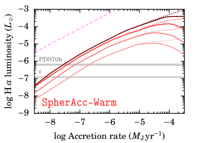
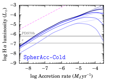
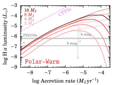
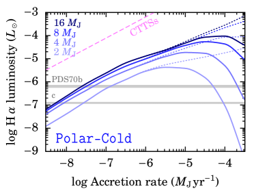
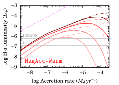
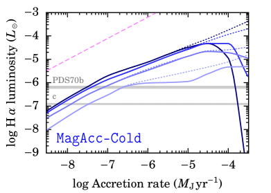
Figure 10: Absorption-modified relationship (solid curves) between H $\alpha$ luminosity and accretion rate for the warm- (left panel) and cold-population (right panel) radius fits for the three accretion geometries (rows; see labels). We consider only absorption by the gas,and also show the case of no absorption (dotted curves). Curves are for masses of 2–16 $M_{\mathrm{J}}$ (bottom to top, but with an inversion in MagAcc-Cold at very high $\dot{M}$). Horizontal bands are for the luminosity of PDS 70 b (Zhou et al., 2021) and PDS 70 c  (Hashimoto et al., 2020). The fit of Ingleby et al. (2013) for CTTSs is also shown (pink dashed line). For reference, one panel shows extinction arrows for $A_{\mathrm{H}\,\alpha}=4$ and 8 mag.

Several authors have studied the empirical correlation between H $\alpha$ luminosity and accretion rate for CTTSs (e.g. Natta et al., 2004; Rigliaco et al., 2012; Ingleby et al., 2013). Recently, this has been extended theoretically to a mass of 6 $M_{\mathrm{J}}$ for the scenario in which the H $\alpha$ is generated by magnetospheric accretion columns (Thanathibodee et al., 2019). In Aoyama et al. (2021), we presented the $\dot{M}$–${L_{\textnormal{H}\,\alpha}}$ correlation for our models for accreting planets, looking also at other hydrogen lines. Here, we briefly present this correlation again but including the effects of absorption. Given the large uncertainty about the dust opacity (Section 5.2), we consider only the gas opacity here.

Aoyama et al. (2020) explained that self-absorption, which occurs in the postshock region (depicted in Figure 2c), lets the scaling of ${L_{\textnormal{H}\,\alpha}}$ with $\dot{M}$ become sub-linear. We find that absorption by the matter flowing onto the planet strengthens this trend and, depending on $f_{\mathrm{fill}}$, can lead to a maximum (“saturation”) luminosity, that is, a flattening and turning over of ${L_{\textnormal{H}\,\alpha}}$ as a function of $\dot{M}$. At low $\dot{M}$, the H $\alpha$ luminosity is intrinsically low, while a high $\dot{M}$ leads both to a higher H $\alpha$ luminosity and to a stronger extinction, with the second effect dominating.

Our $\dot{M}$–${L_{\textnormal{H}\,\alpha}}$ correlation is shown in Figure 10 for $M_{\mathrm{p}}=2$ to 16 $M_{\mathrm{J}}$ for all geometries and both radius fits. For objects with $M_{\mathrm{p}}\lesssim 15\leavevmode\nobreak\ M_{\mathrm{J}}$, the maximum line-integrated luminosity is ${L_{\textnormal{H}\,\alpha,\,\textnormal{max}}}\approx 3\times 10^{-4}\leavevmode\nobreak\ {L_{\odot}}$ in the SpherAcc geometry and ${L_{\textnormal{H}\,\alpha,\,\textnormal{max}}}\approx 10^{-4}\leavevmode\nobreak\ {L_{\odot}}$ in the Polar and MagAcc geometries, reached over a range of accretion rates around $\dot{M}\gtrsim 3\times 10^{-5}\leavevmode\nobreak\ M_{\mathrm{J}}\,\mathrm{yr}^{-1}$. This is relatively insensitive to the choice of the radius fit. Including the extinction by the dust would only lead to a stronger downturn because its importance increases with $\dot{M}$ (see Figure 9).

Interestingly, this implies that for a range of ${L_{\textnormal{H}\,\alpha}}$ values, especially in non-spherically symmetric geometries, there are two solutions to explain a given ${L_{\textnormal{H}\,\alpha}}$ observation: a low $\dot{M}$ without extinction, or a high $\dot{M}$ with extinction. The luminosities of PDS 70 b and c fall precisely in this range of ${L_{\textnormal{H}\,\alpha}}$. We return to this in detail in Section 6.2. The high-$\dot{M}$ solution might be statistically not preferred because observing a planet in a (presumably short) phase of massive accretion is unlikely. Assuming additional amounts of absorption by dust implies accretion rates intermediate between the low and the high solutions.

Could this maximum on the luminosity be responsible for the non-detections of dedicated recent surveys (Cugno et al., 2019; Zurlo et al., 2020; Xie et al., 2020)? Roughly, these surveys typically reached sensitivities down to ${L_{\textnormal{H}\,\alpha}}\sim 10^{-7}$–$10^{-6}\leavevmode\nobreak\ {L_{\odot}}$ beyond 15 au. For most extinction geometries (see Figure 10), this is a few to several orders of magnitude below the peak luminosity. Only for low masses and small filling factors could extinction push a planet into non-detectability, at high accretion rates (in Figure 10, where the dotted lines differ from the solid ones). Closer in to the surveyed stars, where planets are expected to be more numerous (e.g. Bowler, 2016; Fernandes et al., 2019; Nielsen et al., 2019; Vigan et al., 2021), the sensitivity curves become quickly much less constraining; that is, the ${L_{\textnormal{H}\,\alpha}}$ upper limits are higher. In that case, extinction affects only the higher-mass planets, but less than lower-mass planets. The low-mass planets are not detectable in any case. Altogether, extinction by the accreting gas does not appear to be the reason why so few accreting planets have been observed. Other, more likely explanations are discussed in Aoyama et al. (2020) and include the intrinsic rarity of giant planets at the large separations from their host stars to which observations have been sensitive up to now. Depending on the value of the dust opacity (Figure 9), however, the dust could also contribute to hiding accretors. Finally, in general the circumstellar disc could (also) be a source of extinction, to which we return at the end of Section 7.6.

We also briefly compare our absorption-modified $\dot{M}$–${L_{\textnormal{H}\,\alpha}}$ relationship to the fit of Ingleby et al. (2013) for CTTSs. A detailed comparison, including a discussion of the physical differences, is given in Aoyama et al. (2021). Up to $\dot{M}\sim 10^{-5.5}\leavevmode\nobreak\ M_{\mathrm{J}}\,\mathrm{yr}^{-1}$ for SpherAcc and Polar, and up to $\dot{M}\sim 10^{-6.5}\leavevmode\nobreak\ M_{\mathrm{J}}\,\mathrm{yr}^{-1}$ for MagAcc, the slopes are similar between the linear fit and our curves, but with a significant offset of approximately 1.5 dex (several times the spread $\sigma\approx 0.5$ dex of the fit of Ingleby et al. 2013). At large accretion rates, the difference grows dramatically. This implies that a given observed H $\alpha$ luminosity requires much more vigorous accretion in planets than in stars.

6.2 Application to known accreting planets

Robust detections of H $\alpha$ emission from planetary-mass objects exist only for the PDS 70 companions (Wagner et al., 2018; Haffert et al., 2019) and for Delorme 1 (AB)b (Eriksson et al., 2020). The latter, a circumbinary low-mass companion, exhibits hydrogen- and helium-line emission, which is naturally explained by an accretion scenario. The inferred accretion rate onto Delorme 1 (AB)b is $\dot{M}\approx 10^{-9.5}$ or $\approx 10^{-8}\leavevmode\nobreak\ M_{\mathrm{J}}\,\mathrm{yr}^{-1}$, depending on the model used to convert the line luminosities into $\dot{M}$. Even at $\dot{M}\approx 10^{-8}\leavevmode\nobreak\ M_{\mathrm{J}}\,\mathrm{yr}^{-1}$, extinction by either the gas or the dust (Figures 5 or 9, respectively) is entirely negligible.

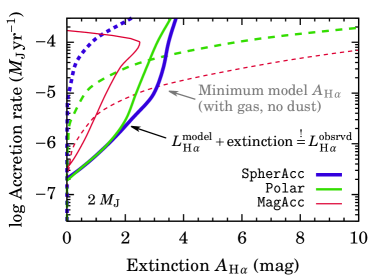
Figure 11: Constraints on the accretion rate onto and total extinction towards PDS 70 b ($M_{\mathrm{p}}\approx 2\leavevmode\nobreak\ M_{\mathrm{J}}$). For a given geometry (line thickness or colour), possible values of $A_{\mathrm{H}\,\alpha}$ are rightward of the dashed line (minimum extinction as a function of $\dot{M}$) and along the solid curve (implied by our emission model and ${L_{\textnormal{H}\,\alpha}}$ from Zhou et al. 2021). Results barely depend on the radius fit (Warm is used here).

We combine the measured luminosity of PDS 70 b with our models to derive joint constraints on the accretion rate and the total amount of extinction. We consider a low mass ($M_{\mathrm{p}}=2\leavevmode\nobreak\ M_{\mathrm{J}}$ for definiteness) as suggested by, for instance, Stolker et al. (2020a) and Wang et al. (2021b), while acknowledging that in $\log(M_{\mathrm{p}})$, the latter study suggests similar probabilities for low and high (logarithmic) masses.

We derive the $\dot{M}$–$A_{\mathrm{H}\,\alpha}$ constraints in two steps. First, we use the measured value of ${L_{\textnormal{H}\,\alpha}}=(6.5\pm 0.9)\times 10^{-7}\leavevmode\nobreak\ {L_{\odot}}$ (Zhou et al., 2021) and draw in Figure 11, for each geometry, the contour of constant extincted ${L_{\textnormal{H}\,\alpha}}$ equal to the observed value (solid lines). This reveals a minimum accretion rate $\dot{M}\approx 2\times 10^{-7}\leavevmode\nobreak\ M_{\mathrm{J}}\,\mathrm{yr}^{-1}$.

Then, we show the extinction $A_{\mathrm{H}\,\alpha}(\dot{M})$ calculated in this work coming only from the gas and without dust, again for each geometry (dashed lines). This is independent of the measured luminosity. The total extinction will therefore be on the line or rightward of it.

Comparing the solid and the dashed line of Figure 11 for each geometry, there is thus only a range of possible accretion rates and extinctions. The maximum $\dot{M}$, set by the crossing of the curves, is near $\dot{M}\approx 3\times 10^{-6}\leavevmode\nobreak\ M_{\mathrm{J}}\,\mathrm{yr}^{-1}$ for MagAcc, near $\dot{M}\approx 3\times 10^{-5}\leavevmode\nobreak\ M_{\mathrm{J}}\,\mathrm{yr}^{-1}$ for Polar, and at higher $\dot{M}$ (slightly beyond the plotted range) for SpherAcc.

In turn, the total extinction (of gas and dust taken together) must be $A_{\mathrm{H}\,\alpha}\lesssim 1$ mag for MagAcc, $\lesssim 3$ mag for Polar, and $\lesssim 4$ mag for SpherAcc. Stronger extinction would leave less flux than observed for any $\dot{M}$. This is broadly consistent with modelling of the NIR SED, which suggests a significant amount of extinction ($A_{\mathrm{H}\,\alpha}\approx 2$–10 mag or more; Hashimoto et al., 2020; Wang et al., 2021b; Cugno et al., 2021). The highest values ($\approx 10$ mag) might not be consistent with our findings ($\lesssim 3$ mag), but this could due to our simplifications in the radiative transfer geometry.

Therefore, the accretion rate onto PDS 70 b is likely $\dot{M}\approx 2\times 10^{-7}$–$10^{-4}\leavevmode\nobreak\ M_{\mathrm{J}}\,\mathrm{yr}^{-1}$. This large spread folds in the uncertainties on the accretion geometry. The results are very similar for $M_{\mathrm{p}}=3\leavevmode\nobreak\ M_{\mathrm{J}}$ or the Cold radius function instead (not shown). This range of $\dot{M}$ is higher than $\dot{M}=10^{-8}\leavevmode\nobreak\ M_{\mathrm{J}}\,\mathrm{yr}^{-1}$ as derived by Haffert et al. (2019), but that was based on a low-mass extrapolation of empirical correlations for stars. Aoyama et al. (2021) found that it is invalid at low masses, as can also be seen in Figure 10 from the discrepancy between the Ingleby et al. (2013) correlation for CTTSs and our curves.

7 Discussion

As Aoyama & Ikoma (2019) point out, the models of Thanathibodee et al. (2019), which are an application of those of Hartmann et al. (1994) to the planetary regime, are premised on the assumption that, as for CTTSs, the H $\alpha$ emission originates in the column(s) of gas accreting onto the planet. Because the heating mechanism of these columns is highly unknown (Muzerolle et al., 2001), these models are parametrised by a maximal temperature $T_{\rm max}$ in the column. Thanathibodee et al. (2019) do not consider emission from the post-shock region, which is appropriate for the stellar case. Thus in Aoyama et al. 2018, Aoyama & Ikoma (2019), Aoyama et al. (2020), and this work, we are exploring a complementary approach. Namely, we are calculating the emission of H $\alpha$ and other lines by the postshock gas, showing that it can be a detectable source, and investigating here the absorption by the accreting material.

Fortunately, the structure of the line-emitting, cooling postshock region is also less uncertain than that of the accretion columns. It would be interesting to deal simultaneously and self-consistently with the emission from the shock itself as well as from the gas and dust accreting onto the planet.

In the following we discuss different aspects of this study or beyond it. We comment on $f_{\mathrm{fill}}$ values (Section 7.1), discuss the time variability of the H $\alpha$ line (Section 7.2), take a critical look at the temperature structure in the accretion flow (Section 7.3), comment on asymmetries in the line profiles (Section 7.4), discuss other sources of extinction (Section 7.5), and relate this work to other recent efforts dealing with extinction (Section 7.6). In Appendix C, we discuss briefly what data exist on other lines for the PDS 70 objects, and what can be learned from this.

7.1 Filling factor values

With no dedicated hydrodynamical simulations of magnetospheric accretion onto planets, we take as rough guidance the values for the filling factor inferred for CTTSs. In the sample by Ingleby et al. (2013), $\approx 80\leavevmode\nobreak\ \%$ of the stars have an estimated global $f_{\mathrm{fill}}<10\leavevmode\nobreak\ \%$, and often amounting to a few percents or fractions of a percent. The same order-of-magnitude estimates have been reported in Calvet & Gullbring (1998), with there $f_{\mathrm{fill}}$ typically less than 10 %, using spectroscopic data. More recently, Robinson & Espaillat (2019) similarly found filling factors of tens of percent for a few objects from HST low-resolution observations. Estimates derived from multi-wavelength time-series photometry can be less precise, but they also indicate typically $f_{\mathrm{fill}}<10\leavevmode\nobreak\ \%$–20 % for the bulk of CTTSs dominated by hot accretion spots (e.g. Bouvier et al., 1993, 1995; Venuti et al., 2015).

In this study, we have assumed that the accretion occurs only over one or several region(s) with $\dot{M}\neq 0$, while $\dot{M}=0$ outside of this. More realistically, there will be a distibution of local accretion rates covering different fractions of the surface as for CTTSs (e.g. Bouvier et al., 2007; Ingleby et al., 2013). The resulting line profile in this case could be a linear combination of the profiles for each hot spot, but geometrical effects (not all spots being radially directly towards the observer) will complicate this picture.

Using the Hartmann et al. (1994) model, Thanathibodee et al. (2019) describe the magnetospheric accretion flow as originating from the CPD between the inner (or truncation) radius $R_{\mathrm{i}}$ and the outer radius $R_{\mathrm{o}}=R_{\mathrm{i}}+W_{r}$, where $W_{r}$ is the width of the flow at the launching point. With these definitions, the axisymmetric angles on the planet covered by accretion are given by $\sin^{2}\theta_{\mathrm{i},\mathrm{o}}=R_{\mathrm{p}}/R_{\mathrm{i},\mathrm{o}}$ (Hartmann et al., 1994). From Equation (1), the filling factor is

$$f_{\mathrm{fill}}=\sqrt{1-\frac{R_{\mathrm{p}}}{R_{\mathrm{i}}+W_{\mathrm{r}}}}-\sqrt{1-\frac{R_{\mathrm{p}}}{R_{\mathrm{i}}}}.$$ (23)

Thanathibodee et al. (2019) consider a range of $R_{i}=(2$–8$)\leavevmode\nobreak\ R_{\mathrm{p}}$ and $W_{r}=(1$–$6)\leavevmode\nobreak\ R_{\mathrm{p}}$, which corresponds to $f_{\mathrm{fill}}=1$ %–20 %. They find a roughly flat distribution of $R_{\mathrm{i}}$ and $W_{\mathrm{r}}$ matching the observed fluxes for PDS 70 b and PDS 70 c. This corresponds also to the range we consider in this work.

7.2 Time variability

Time variability in the H $\alpha$ flux (and in other lines and filters as well) is a well-known phenomenon for CTTSs (e.g. Herbst et al., 1994; Siwak et al., 2018). Monitoring campaigns of their accretion variability showed that this is typically dominated by the timescale of rotational modulation of the accretion features (e.g. Costigan et al., 2014), that is usually of the order of 0.5–2 weeks (e.g. Roquette et al., 2017). If we exclude the most “extreme” cases (for instance, unstable accretors), which can exhibit prominent variations over timescales of hours, the amplitude of the $\dot{M}$ variability on CTTSs is typically observed to increase from timescales of hours to timescales of days, and then flatten out and remain approximately constant over timescales as long as years (Costigan et al., 2014; Sergison et al., 2020). This indicates that the global structure of accretion persists over hundreds of rotational cycles, albeit with smaller-scale variations on shorter timescales (e.g. Grankin et al., 2007). The typical $\dot{M}$ variability measured on week-long timescales is $\approx 0.4$–0.5 dex (Costigan et al., 2014; Venuti et al., 2014), out of which $\approx 70\leavevmode\nobreak\ \%$ can be explained in terms of geometric modulation of the accretion shock. This implies that the intrinsic $\dot{M}$ variability on such timescales typically amounts to only $\approx 0.15$ dex. Also, radiation-magnetohydrodynamical simulations of CTTSs (e.g. Kurosawa & Romanova, 2013) indeed find that both stable and unstable accretors have stochastically changing line profiles, with paradoxically a more stationary appearance of the line profile for unstable accretors. The estimate of Thanathibodee et al. (2020) for the variability of $\dot{M}$ onto the PDS 70 star, 0.56 dex over the rotation cycle, is indeed consistent with these typical estimates of accretion variability for CTTSs. Time variability has also been seen in low-mass brown dwarfs, for example in the $\approx 47\leavevmode\nobreak\ M_{\mathrm{J}}$, $\approx 1$-Myr-old brown dwarf candidate DENIS 1538–1038 (Nguyen-Thanh et al., 2020).

For the planetary regime studied here, in the case of magnetospheric accretion, time variability in the strength of the accretion tracer can come from (at least) the following:

• from variations of the accretion rate onto the planet, which might be on the keplerian timescale around it, $P\sim 2\leavevmode\nobreak\ \mathrm{d}\times[R/(10\leavevmode\nobreak\ R_{\mathrm{J}})]^{3/2}[M_{\mathrm{p}}/(3\leavevmode\nobreak\ M_{\mathrm{J}})]^{-1/2}$ at cylindrical radius $R$;

• from variations of the magnetic field topology, with a timescale linked to the one over which the field-generating gas in the planet’s interior moves;

• from variations of the viewing angle onto the hot spot (through the column or not), over the course of a planetary rotation ($\sim 10$ h; Snellen et al., 2014; Bryan et al., 2018, 2020; Wang et al., 2021a); and

• from variations of the optical depth along the column, for example from fluctuations in the temperature structure. If the preshock region is transmissive (“optically thin”), its thermal time should set the timescale (Malygin et al., 2017); otherwise, the diffusion time is the relevant quantity. Simple estimates of their value is however challenging, but they are likely fast compared to the other, dynamical processes.

Concerning point (iii): it is not clear whether the light emitted at the shock needs to pass through the accretion column, as we have assumed here; this might be the case only at certain phases.

Zhou et al. (2021) recently detected PDS 70 b at H $\alpha$ and the UV continuum ($U$ band) with HST at several epochs over five months, separated typically by weeks, and found no statistical evidence for variability in H $\alpha$ beyond the $\sim 10$ % level. These timescales correspond to the orbital period at tens of $R_{\mathrm{J}}$ from the planet (see item (i) above). Constraints on variability of the signal on the timescale of a possible planet rotation would be a valuable extension.

It is not clear how to disentangle the variation in the signal coming from optical-depth effects and from accretion-rate variations. Variability in the accretion rate (item (i) above) is expected over a wide range of timescales but it decreases towards short timescales (Gárate et al., 2021). Therefore, the accretion rate might show only small variations over a rotational period, but both high-resolution simulations and monitoring campaigns will be needed to assess this in detail. Also, if the accretion rate and mass are such that extinction is absent or negligible, variations in the H $\alpha$ signal would be due only to variations in the accretion rate, for instance due to episodic accretion (Lubow & Martin, 2012; Brittain et al., 2020; Martin et al., 2021), which might not be periodic, or to rotational modulation of the accretion features (e.g. hot spots), which would be periodic. Ideally, this could help distinguish the source of the variability while providing constraints on the spin rate of young objects (Bryan et al., 2018; Ginzburg & Chiang, 2020; Bryan et al., 2020).

7.3 Temperature structure

Our assumption that the temperature decreases away from the accreting object finds support in the empirical determination by Petrov et al. (2014) for a CTTS using line ratios probing different sections of the accretion column, and agrees with the self-consistent model of Martin (1996). This temperature distribution contrasts with the one assumed in the models of Hartmann et al. (1994) and Muzerolle et al. (1998, 2001) (see brief review in Bouvier et al. 2007), which Thanathibodee et al. (2019) use, and their more recent developments (e.g. Lima et al., 2010). There, the temperature profile scales everywhere inversely with the density, and the maximum temperature is a free parameter. Hartmann et al. (2016) suggest that magnetic effects could play a role in setting the temperature structure but this remains unknown. Thus our approximation is a possible one but its validity is currently difficult to assess.

7.4 Line asymmetries

When the line profile becomes asymmetric because of non-uniform absorption (see Figures 6, 7, and 8), a shift of the line peak ensues, generally to the blue side. This is typically around $|\Delta v|\approx 20\leavevmode\nobreak\ \mathrm{km}\,\mathrm{s^{-1}}$. While this is only a fraction of the resolution of MUSE (FWHM of 120 $\mathrm{km}\,\mathrm{s^{-1}}$), it is possible to determine the line centroid better than a resolution element. Indeed, Haffert et al. (2019) reported shifts of $\Delta v=25\pm 8$ and $30\pm 9$ $\mathrm{km}\,\mathrm{s^{-1}}$ for PDS 70 b and c relative to the star, towards the red side. It seems to have the opposite sign relative to the models. However, this was with respect to the stellar H $\alpha$, which has an asymmetric line profile. Thus the signal itself could still be overall blue-shifted.

If there is any, the redshifted resonant absorption should be at a clearly larger velocity offset (see Figure 8) than the Keplerian speed of the planet on its orbit around its host, which is $v_{\mathrm{K}}=9.4\leavevmode\nobreak\ \mathrm{km}\,\mathrm{s^{-1}}\times\sqrt{{M_{\star,\,1}}/a_{10}}$ for a circular orbit, where ${M_{\star,\,1}}\equiv{M_{\star}}/(1\leavevmode\nobreak\ {M_{\odot}})$ and $a_{10}\equiv a/(10\leavevmode\nobreak\ \mathrm{au})$. Thus the orbital motion will not be able to shift significantly the absorption at the central rest wavelength of H $\alpha$. Similarly, the spin broadening should not be important for the line shape as a whole since young planets have equatorial spin velocities of order $v\approx 10\leavevmode\nobreak\ \mathrm{km}\,\mathrm{s^{-1}}$ (Snellen et al., 2014; Bryan et al., 2018, 2020; Wang et al., 2021a), which is much narrower than the line. However, the fine spectral features seen for the warm-population radii in the Polar or the MagAcc case (Figures 7 and 8b, respectively) would possibly be more challenging to distinguish. On the other hand, this depends on the latitude from which the line is emitted.

Note that, puzzlingly, the line profiles of Thanathibodee et al. (2019) do not display a redshift despite the free-fall velocities that they should be obtaining where the emission is maximal, judging from the equivalent problem for CTTSs in Hartmann et al. (1994).

7.5 Other possible sources of extinction

In this work, we have dealt only with the extinction due to the material in the accretion flow within the Hill sphere of the planet. The contribution from the ISM is in principle easy to estimate from the stellar SED. In this section, we discuss other sources, looking at PDS 70 b as an example.

The PDS 70 planets have been found inside a large cavity (whose size depends on wavelength; Hashimoto et al., 2015; Keppler et al., 2018; Long et al., 2018; Isella et al., 2019) that seems to be devoid of gas and dust, except for some small amounts of various optically thin molecules (Facchini et al., 2021). To model the CSD of PDS 70, Bae et al. (2019) and Toci et al. (2020) have an azimuthally averaged gas column density of $\Sigma\sim 10^{-3}$ cm² g^-1 at the location of PDS 70 b. From Figure 9c, $A_{R}\approx\kappa_{\mathrm{dust,\,H}\,\alpha}\Sigma\sim 10^{-4}$–0.1 mag. This suggests that the CSD should not lead to any significant extinction. Finally, PDS 70 c could be affected more severely by extinction because of its proximity to the gap edge (Haffert et al., 2019). However, the extinction at ALMA wavelengths is not strong enough as to prevent the detection of a CPD around PDS 70 c (Benisty et al., 2021).

Given the inclination of $i=52{\mbox{\textdegree}}$ (Keppler et al., 2019), the emission from the planet passes through a significant fraction of the column density only if the CPD has an aspect ratio greater than approximately $\arctan(i)\approx 0.7$. Gressel et al. (2013) found such thick discs for masses $M_{\mathrm{p}}\sim 0.3\leavevmode\nobreak\ M_{\mathrm{J}}$ and Ayliffe & Bate (2009) found thinner discs with an aspect ratio $\lesssim 0.4$, decreasing with increasing mass. Given that PDS 70 b cannot be too light in order to still emit H $\alpha$, its CPD is likely sufficiently thin to not absorb significantly.

If the H $\alpha$ is generated on the CPD surface, the inclination will lead to a higher optical depth by a factor of only $\approx 1/\cos i=1.6$ since the disc is not too edge-on. Thus, it seems realistic that the CPD and CSD material does not contribute to the absorption, especially for PDS 70 b, which is found in a gap. Only for PDS 70 c (close to the gap rim) could there be an effect, especially at short wavelengths such as H $\alpha$ and H $\beta$.

As mentioned by Aoyama & Ikoma (2019), absorption could in general be due to a disc wind. This wind could be dusty, with the radiation pressure playing a key role and the dust porosity and size evolving significantly while being transported by the wind (Vinković & Čemeljić, 2021). Thanathibodee et al. (2020) find that the mass-loss rate in the wind of PDS 70 is $\dot{M}_{\mathrm{wind}}\sim 10^{-11}\leavevmode\nobreak\ {M_{\odot}}\,\mathrm{yr}^{-1}\sim 10^{-8}\leavevmode\nobreak\ M_{\mathrm{J}}\,\mathrm{yr}^{-1}$, which might lead to a very small surface density given the large area over which it is spread. However, estimating the absorption by a disc wind in detail is well beyond the scope of this work.

Finally, the reduction in the surface density at the location of the planet depends on the viscosity, which is still a mostly unconstrained parameter of CSDs. Thus it possible for the disc column density above the planet to be negligible for a given accretion rate. We note that a non-extinguishing gas and dust surface density is one of the arguments made in the “massive accreting gap planet” model of Close (2020). In summary, the case of no absorption by the CSD is a useful limit.

7.6 Relation to other theoretical work dealing with extinction

The recent theoretical study of Sanchis et al. (2020) also deals with the absorption of the flux from a planet by material in the system. Our approaches are similar but distinct: they use interstellar medium (ISM) dust opacity values (we attempt to estimate them specifically for accretion onto planets, and consider also absorption by the gas) to address the extinction in different infrared filters (we deal with one accretion line). The flow geometry is handled differently (in 3D in their case, albeit with a non-zero smoothing length), the parameter space is surveyed to a different extent (more broadly in our case, and with $\dot{M}$ and $M_{\mathrm{p}}$ independent), and the thermodynamics are treated differently (they assume isothermal gas, while we take the radiation transport into account), while the radiative transfer is similar in both. Thus in many respects the study of Sanchis et al. (2020) and ours are complementary.

Sanchis et al. (2020) performed hydrodynamics simulations for specific stellar and planetary parameters, but being isothermal, their simulations can be rescaled (approximately; see their Section 3.2.3) to apply to other values. For PDS 70 b, using a gas surface density from Keppler et al. (2018) and scaling to the stellar mass of ${M_{\star}}\approx 0.8\leavevmode\nobreak\ {M_{\odot}}$, they considered masses of $M_{\mathrm{p}}=0.5$–2.4 $M_{\mathrm{J}}$ and accretion rates $\dot{M}=(2$–$3)\times 10^{-8}\leavevmode\nobreak\ M_{\mathrm{J}}\,\mathrm{yr}^{-1}$. This $\dot{M}$ is dictated by the rescaling of their simulations through (E. Sanchis 2021, pers. comm.)

$$\dot{M}^{\prime}=\dot{M}\left(\frac{a}{a^{\prime}}\right)^{3}\frac{\Sigma_{1}^{\prime}}{\Sigma_{1}}\sqrt{\frac{{M_{\star}}^{\prime}}{{M_{\star}}}},$$ (24)

where non-primed quantities are the ones used in the actual simulations and primed quantities the rescaled ones, with $a$ the semimajor axis of the planet and $\Sigma_{1}$ the surface density at a fixed reference semimajor axis, for instance 1 au. For $(a,a^{\prime})=(5.2,22)$ au, $(\Sigma_{1},\Sigma_{1}^{\prime})=(290,12.5)$ g cm^-2 (at 1 au), and $({M_{\star}},{M_{\star}}^{\prime})=(1.6,0.76)\leavevmode\nobreak\ {M_{\odot}}$ as appropriate for their parameter choices for PDS 70 b at 22 au, Equation (24) yields $\dot{M}^{\prime}/\dot{M}=3.92\times 10^{-4}$, that is, $\dot{M}^{\prime}=(2$–$3)\times 10^{-8}\leavevmode\nobreak\ M_{\mathrm{J}}\,\mathrm{yr}^{-1}$. This is a somewhat low, but reasonable value.

We can derive the H $\alpha$ extinction that Sanchis et al. (2020) would predict and compare this to our results. They obtained $K$-band extinctions $A_{K}=0.74$, 0.22, and 0.0030 mag for $M_{\mathrm{p}}=0.48$, 0.95, and 2.38 $M_{\mathrm{J}}$ respectively (E. Sanchis 2021, pers. comm.). With the opacity law they used (Cardelli et al., 1989), this translates to $A_{\mathrm{H}\,\alpha}\approx 5.3$, 1.6, and 0.021 mag respectively.

The dependence on the planet mass is thus very strong: the extinction varies from $A_{\mathrm{H}\,\alpha}\approx 5$ to 0.02 mag despite a change of only a factor of $\approx 2.5$ in mass, for essentially the same accretion rate. This seemingly does not agree with our results, in which the extinction decreases much more slowly with mass: $A_{\mathrm{H}\,\alpha}\propto\Sigma$, and $\Sigma\propto M_{\mathrm{p}}^{-0.5}$ approximately (Equation (17)). However, this holds for a fixed accretion geometry, and in their case higher-mass planets open a deeper gap, with a surface density above the planet reduced by a factor of $\approx 2$ between the 0.48- and 0.95-$M_{\mathrm{J}}$ simulations ($\Sigma\sim M_{\mathrm{p}}^{-1}$), and of ten between the 0.95- and 2.38-$M_{\mathrm{J}}$ simulations ($\Sigma\sim M_{\mathrm{p}}^{-2.5}$). The velocity is certainly not larger than the smoothing-free free-fall velocity from infinity we assume and, in fact, because of the gravitational smoothing, is likely much smaller. Therefore, to have the same $\dot{M}$ despite a reduced density above the planet, the gas must be accreting nearer to the equator in their case. Thus our assumption that the shock radiation passes entirely through the accretion flow (Figure 1) does not apply to their simulations and indeed provides an upper limit on the amount of absorption. This is an important aspect of the quantitative differences.

Another aspect is that Sanchis et al. (2020) calculate the extinguishing column density from a distance $r=0.03$–$0.1\leavevmode\nobreak\ {R_{\textnormal{Hill}}}$ outwards from the planet, due to the smoothing. Given the rescaling, for PDS 70 b at 22 au this corresponds to $r=80$, 340, and $\approx 200\leavevmode\nobreak\ R_{\mathrm{J}}$ as a starting radius for the integration for the $M_{\mathrm{p}}=0.48$, 0.95, and 2.48 $M_{\mathrm{J}}$ simulations. Thus, their column densities are smaller than what higher-resolution simulations would yield. Nevertheless, the qualitative result of a decreasing extinction with increasing mass should be robust.

The work of Szulágyi & Ercolano (2020) deals with the emission of hydrogen lines by accreting planets and the absorption of these lines by the surrounding gas. We discuss their approach to calculating the emission in Aoyama et al. (2021) and assess in Aoyama et al. (2020) the applicability of Storey & Hummer (1995), which Szulágyi & Ercolano (2020) used, to the planetary accretion shock.

Here, we comment briefly on the relation between Szulágyi & Ercolano (2020) and this work. As for the comparison to Sanchis et al. (2020), our approaches are in principle similar, with the major advantage of Szulágyi & Ercolano (2020) that they too consider an intrinsically 3D gas structure, from the three-dimensional simulations of Szulágyi et al. (2016). As we have shown in Figure 9, the dust opacities of Szulágyi & Ercolano (2020) per gram of dust are consistent with the range that we consider as more likely, with a different net result because of our much lower assumed dust-to-gas mass ratio ($f_{\textrm{d/g}}\sim 10^{-5}$–$10^{-3.5}$ instead of $f_{\textrm{d/g}}=10^{-2}$ in their case).

The main difference between Szulágyi & Ercolano (2020) and this work is again in the density structure, which is affected by the need to use a non-zero gravitational smoothing length ($\sim$ fraction of ${R_{\textnormal{Hill}}}$) and large grid cells ($\sim R_{\mathrm{J}}$), due to the fact that these are three-dimensional, global-disc and thus numerically expensive simulations. Judging by the density structures seen in their Figure 4, there is likely also a considerable amount of variability. Consequently, estimating the mean influx rate would require dozens of snapshots. Therefore, the extinction might be calculated more accurately in our work but our density structure is simplified and thus approximate, albeit in a different way. The reader is refered to Appendix B of Aoyama et al. (2020) and also Aoyama et al. (2021) for the more important discussion of how the emission was computed in Szulágyi & Ercolano (2020).

Altogether, in Sanchis et al. (2020) or Szulágyi & Ercolano (2020) the flow is not correctly captured from small scales downwards in their simulations (at best a few tens of $R_{\mathrm{J}}$; corresponding to medium scales downwards in our model). This implies that those studies cannot study reliably the contribution of the accretion flow to the extinction as we have done here.

8 Summary and conclusions

Motivated by recent detections of accreting planets and by the non-detections from surveys at H $\alpha$, we have studied to what extent the gas and dust accreting onto a forming planet can absorb the H $\alpha$ emission coming from the shock at the planet surface, and what the spectral signatures of this extinction might be.

We surveyed the large parameter space of planet properties and considered three accretion geometries: spherical, polar, and magnetospheric (Section 3.1). For each parameter combination, we integrated the equation of radiative transfer along the accretion flow. This integration is needed because of the strong wavelength, density, and temperature dependence of the gas opacity (Figure 3).

The main take-aways of this study are the following:

1. The accreting gas absorbs the line-integrated flux with 0.5 mag or more only for accretion rates $\dot{M}\gtrsim 3\times 10^{-5}\leavevmode\nobreak\ M_{\mathrm{J}}\,\mathrm{yr}^{-1}$ in spherical symmetry (SpherAcc) or $\dot{M}\gtrsim 3\times 10^{-6}\leavevmode\nobreak\ M_{\mathrm{J}}\,\mathrm{yr}^{-1}$ for polar accretion, with a weak mass dependence (Figure 5). In the MagAcc case the mass dependence is stronger. Except for MagAcc-Cold, the amount of extinction increases towards smaller masses. This is partly due to the increase in density with decreasing planet mass at a given $\dot{M}$ (see Equation (3)). Another reason is that the opacity happens mostly to increase with decreasing mass (see Figure 3). Up to $\dot{M}\approx 3\times 10^{-4}\leavevmode\nobreak\ M_{\mathrm{J}}\,\mathrm{yr}^{-1}$ and for masses above $M_{\mathrm{p}}=10\leavevmode\nobreak\ M_{\mathrm{J}}$, the gas absorbs with at most $A_{\mathrm{H}\,\alpha}\lesssim 4$ mag in the SpherAcc and Polar geometries.

2. At low $\dot{M}$, the observed line profile is the same as the one leaving the planet, but moderate to high $\dot{M}$ values lead to clear spectral features. There is no systematic trend in these features because they are due to several molecular and atomic lines. Larger amounts of extinction tend to be associated with a “spiky” spectrum showing features visible at a resolution of 10–20 $\mathrm{km}\,\mathrm{s^{-1}}$ ($R\gtrsim 15,000$; Figure 8) and suggest relatively localised absorption, as could occur in a magnetospheric accretion geometry.

3. Larger-scale ($\Delta v\sim 100\leavevmode\nobreak\ \mathrm{km}\,\mathrm{s^{-1}}$) slopes in the gas opacity at H $\alpha$ introduce asymmetries in the line shape. This is often more important than asymmetries in the line emerging from the shock.

4. Based on the recent literature, we estimated that the accreting dust has an extinction curve shallower than in the ISM (Cardelli et al., 1989; Wang & Chen, 2019). A conservative range of opacity values at H $\alpha$ is $\kappa_{\mathrm{dust,\,H}\,\alpha}\sim 10^{-2}$–$10$ cm² g${}^{-1}_{\textrm{gas}}$ at $f_{\textrm{d/g}}\sim 10^{-5}$–$3\times 10^{-4}$ (Figure 9), which is 10–$10^{4}$ times lower than in the ISM. Our dust opacity implies that for most parameter combinations the absorption by the dust is negligible to small (Section 5.4).

5. For a given planet mass there is a maximal H $\alpha$ luminosity because absorption increases more strongly with $\dot{M}$ than ${L_{\textnormal{H}\,\alpha}}$ does (Figure 10). Considering only the gas opacity, this maximum is ${L_{\textnormal{H}\,\alpha}}\approx 10^{-4}\leavevmode\nobreak\ {L_{\odot}}$ for $M_{\mathrm{p}}\sim 10\leavevmode\nobreak\ M_{\mathrm{J}}$. Lower masses peak at lower ${L_{\textnormal{H}\,\alpha}}$. Therefore, for certain values, an ${L_{\textnormal{H}\,\alpha}}$ measurement can be interpreted as two different accretion rates, a low or a high value. Also considering some dust absorption implies $\dot{M}$ values between the two extremes.

6. The current computational capacities impose a coarse spatial resolution of the flow near the planet in multidimensional studies. This affects dramatically their estimate of the flow’s contribution to the absorption (Section 7.6). This highlights the complementarity of our approach, which assumes a simplified geometry but more realistic densities, temperatures, and velocities in the accretion flow and at the shock.

7. The accretion rate onto Delorme 1 (AB)b is much too low for absorption by gas or dust in the accretion flow to matter (Section 6.2). For PDS 70 b, we used the indication of a low mass and the observed luminosity to derive from our models a range of possible accretion rates and extinctions. We found $10^{-7}\lesssim(\dot{M}/M_{\mathrm{J}}\,\mathrm{yr}^{-1})\lesssim 10^{-4}$ and $A_{\mathrm{H}\,\alpha}\lesssim 4$ mag ($A_{V}\lesssim 5$ mag).

Thus, for planets found in gaps (i.e. when the surface density of the circumstellar disc is negligible), it may not be necessary to correct for any extinction at H $\alpha$ within the system. It also suggests that the paucity of detected planets might not be mainly due to heavy extinction by the accreting material but rather to a less efficient conversion of the accretion energy to H $\alpha$ than for CTTSs (Aoyama et al., 2021).

We note that for a shock on a CPD, compared to the shock on a the planet surface, at a given total accretion rate the mass flux is spread over a much larger area, so that the absorption will likely be essentially zero. Thus the H $\alpha$ line should be smooth and shaped only by the postshock region.

The complexity of the problem, due to uncertainties in the accretion geometry and the dust opacity, will make detailed modelling of individual objects enlightening. Obtaining high-resolution spectra will be an important breakthrough to overcome the limitations of MUSE, from which only upper limits on the line width can be set. With high-resolution spectra, our grid of line shapes could be used to perfom fits to the observed line profile, using the total flux also as a fit criterion, and ideally fitting at the same time other accretion tracers such as H $\beta$, Pa $\beta$, Pa $\alpha$, Br $\gamma$, Br $\alpha$, or metal lines.

Appendix A Including the emission from the infalling matter

We assess to what extent the emission by the accreting gas and dust can be neglected. Keeping the emission term, the formal solution of the radiative transfer equation (Equation (11)) reads at a given wavelength (omitting the $\lambda$ subscript)

$$I(\tau)=I({\tau_{\mathrm{max}}})e^{-{\tau_{\mathrm{max}}}-\tau}+\int_{\tau}^{\tau_{\mathrm{max}}}S(\tau^{\prime})e^{-(\tau^{\prime}-\tau)}d\tau^{\prime},$$ (25)

where $S$ is the source function, $I$ is the outward intensity, and $\tau$ is the inward optical depth with $\tau=0$ formally at $r=\infty$ (at the observer) and $\tau={\tau_{\mathrm{max}}}$ at the shock (the surface of the planet). Therefore, the intensity at the observer is, for a purely radial ray,

$$I(\tau=0)=I({\tau_{\mathrm{max}}})e^{-{\tau_{\mathrm{max}}}}+\int_{0}^{\tau_{\mathrm{max}}}S(\tau^{\prime})e^{-\tau^{\prime}}d\tau^{\prime},$$ (26)

so that, neglecting limb darkening, the luminosity at the observer is given simply by $L=4\pi R_{\mathrm{p}}^{2}\times\pi I(\tau=0)$. The emerging intensity is made up of the attenuated intensity from the shock (first term) and the weighted integral of the source function (second term). Assuming LTE, $S=B$ is a known function if the density, opacity, and temperature profiles are given, as we do assume here, making it possible to compute the integral in Equation (26). For simplicity in this work, we have kept only the first term in Equation (26) (compare to Equation (14c)). However, for large total optical depths ${\tau_{\mathrm{max}}}$, it can become negligible relative to the emission term.

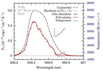
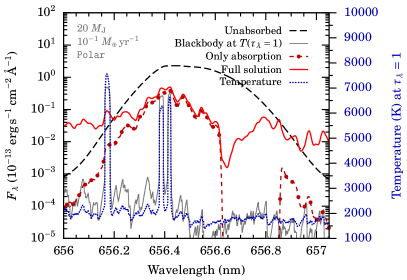
Figure 12: Full solution to the radiative transfer approximation (Equation (11)) including the emission term (see Equation (26)) compared with the approximate, absorption-only solution (Equation (14c)). We show the flux leaving the planet (dashed black line), the solution taking only absorption into account (dark red dashed line with dots), and the full solution (pale red full line), as well as the source function (blackbody intensity) at the location where $\tau_{\lambda}=1$ radially inwards (grey line), for those wavelengths where $\tau_{\lambda}=1$ is reached. The temperature of the blackbody there is shown against the right axis (blue dotted line). Left panel: Case of Figure 4. The strong preshock absorption at the Doppler-shifted H $\alpha$ resonance near the planet is filled in somewhat by the emission in the accretion flow, almost to the level of the blackbody at $\tau_{\lambda}=1$, roughly according to the Milne–Barbier–Unsöld relationship. Right panel: Case of polar accretion for $\dot{M}=3\times 10^{-4}\leavevmode\nobreak\ M_{\mathrm{J}}\,\mathrm{yr}^{-1}$, $M_{\mathrm{p}}=20\leavevmode\nobreak\ M_{\mathrm{J}}$ for the cold-population radius fit ($R_{\mathrm{p}}=3.4\leavevmode\nobreak\ R_{\mathrm{J}}$). Outside of the line centre, the outcoming intensity is much higher than the source function at $\tau_{\lambda}=1$ and thus the full solution is not roughly the sum of the absorption-only curve and the source function at $\tau_{\lambda}=1$.

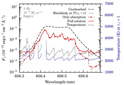
Figure 13: As in Figure 12, but for a case from MagAcc (top left in Figure 8b). The emission from the accreting material region is important only in the far wings.

We show in Figure 12 the result of including the emission term for two examples. This is compared to the correction provided by the Barbier–Eddington (perhaps more accurately “Milne–Barbier–Unsöld”; see a rewiew of its history in Paletou 2018) relationship. It states that the emerging intensity, less the first term in Equation (26), is equal to the value of the source function at a depth $\tau=1$. Importantly, the derivation assumes that the source function is a linear function of the optical depth: $S=a+b\tau$, for constant $a$ and $b$.

In the first case (Figure 12a), which uses the parameters of Figure 4, the full solution is practically identical with the absorption-only solution, except at the strong absorption caused by the Doppler-shifted H $\alpha$ resonance near the planet at $\lambda\approx 656.7$–656.8 nm (see the solid yellow region in Figure 4). The Barbier–Eddington or Milne–Barbier–Unsöld correction (MBU; grey line) is non-zero only there because the total optical depth at the other wavelengths is less than unity. This correction is only some 20–70 % away from the full solution and thus yields a reasonable approximation. The full solution is lower than predicted by the MBU relationship, implying that the observable intensity effectively comes from a region of lower temperature and therefore lower optical depth. This is because the source function, a blackbody, is a monotonic function of the temperature and the temperature increases with increasing optical depth (decreasing radius).

In the second example (Figure 12b), the absorption-only curve profile is 1–2 dex fainter than the flux at the planet’s surface (i.e. $\tau_{\lambda}\approx 2$–4) outside of the resonance, where the flux is effectively zero. For most of the range shown, the source function at $\tau_{\lambda}=1$ is orders of magnitude smaller than the absorption-only curve. However, in the full solution the flux can be as high as the absorption-only line (near the centre) or even much higher (in the wings, including the Doppler-shifted resonance). Where it is much higher, the MBU relationship can be seen not to hold. The reason is that the source function is a strongly non-linear function of the optical depth: it—or more relevantly the emissivity $j_{\lambda}=\alpha_{\lambda}S_{\lambda}=\alpha_{\lambda}B_{\lambda}$—is nearly zero from $\tau_{\lambda}=0$ to an optical depth $\tau_{\lambda}>1$, where it rises sharply. Thus the emission mostly comes from a depth with a high blackbody temperature. For example, at $\lambda=656.0$ nm, this transition occurs at $\tau_{\lambda}=1.8$, and the source function at $\tau_{\lambda}=1.89$ is equal to the outcoming intensity.

Since in Figure 12b the extinction structure of the flow does not depend too much on wavelength, the resulting line shape is relatively flat, within a factor of ten. The only exceptions are near the line peak, where the attenuated shock flux (first term of Equation (26)) is important, and in the blue part of the Doppler-shifted H $\alpha$ resonance, where the emission is noticeably less strong. Also, in the narrow opacity window at $\lambda=656.17$ nm the outcoming flux is smaller by 1 dex than that coming from a blackbody at $T(\tau_{\lambda}=1)\approx 7500$ K, whereas near 656.37 and 656.42 nm the observable flux is indeed approximately equal to the sum of the extincted flux from the planet surface and that of a blackbody at $T(\tau_{\lambda}=1)$.

A further example is provided in Figure 13, now for $\dot{M}=3\times 10^{-5}\leavevmode\nobreak\ M_{\mathrm{J}}\,\mathrm{yr}^{-1}$, $M_{\mathrm{p}}=5\leavevmode\nobreak\ M_{\mathrm{J}}$ in the warm population ($R_{\mathrm{p}}=4.5\leavevmode\nobreak\ R_{\mathrm{J}}$). The absorption-only line matches the full solution everywhere except in the outer parts of the line. This is however visible only because the fluxes are displayed on a logarithmic scale; in reality it is only a very small difference.

The example of Figure 12b is an extreme one (very high accretion rate and mass), and in most cases the emission by the gas accreting onto the planet is negligible. When the optical depth to the planet is not very large, the extincted shock flux will likely dominate over the emission from the accretion flow. Near the line wings, emission from the accretion flow emission or the planet’s can become important, leading to an apparently narrower line, but this should be generally only a small correction because the shock (peak or total) flux is large.

Appendix B Line profiles for the cold-population radii

Figures 14 and 15 show a grid of line profiles for the SpherAcc-Cold and the Polar-Cold scenarios, as in Figures 6 and 7 respectively. See the description in Section 4.3. The MagAcc-Cold line profiles are shown in Figure 8.

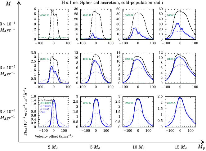
Figure 14: As in Figure 6, but for SpherAcc-Cold.

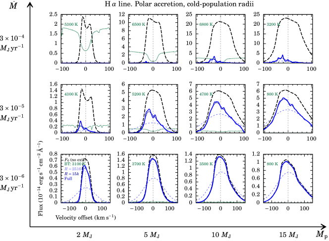
Figure 15: As in Figure 6, but for Polar-Cold.

Appendix C Using measurements of other lines

In this section, we briefly recall the upper limits available on the fluxes of lines other than H $\alpha$, and derive from the H $\beta$ upper limit of Hashimoto et al. (2020) constraints on the total extinction. We follow the approach of Hashimoto et al. (2020) but provide the expression for the extinction explicitly.

Stolker et al. (2020a) recovered for the first time PDS 70 b in the narrow filter NB4.05 of VLT/NACO centred at Br $\alpha$ ($\lambda_{\mathrm{c}}=4.05\leavevmode\nobreak\ \upmu$m, effective width $\Delta\lambda=0.0616\leavevmode\nobreak\ \upmu$m) as part of the MIRACLES survey (Stolker et al. 2020b). However, there is no evidence for a shock excess at NB4.05, where the thermal emission from the atmosphere is significant. Also, using VLT/SINFONI, Christiaens et al. (2019) and Wang et al. (2021b) did not detect a shock excess in Br $\gamma$ at 2.166 $\upmu$m, nor did Uyama et al. (2021) in Pa $\beta$ with Keck/OSIRIS. We note that this is consistent with the models of Aoyama et al. (2020), which predict that these lines should be much lower than the photospheric emission. The moderate resolution of the instruments dilutes any shock excess into the continuum.

The measured upper limit on the flux ratio between H $\beta$ and H $\alpha$, $\varphi_{\textnormal{obs}}$, can be converted to a lower limit on $A_{\mathrm{H}\,\alpha}$ through

$$A_{\mathrm{H}\,\alpha}>2.5\leavevmode\nobreak\ \mathrm{mag}\times\frac{\log_{10}\left(\varphi_{\textnormal{theo,\,surf}}/\varphi_{\textnormal{obs}}\right)}{\left(\lambda_{\mathrm{H}\,\alpha}/\lambda_{\mathrm{H}\,\beta}\right)^{-p_{\textnormal{UV}}}-1},$$ (27)

where $p_{\textnormal{UV}}=\Delta\log\kappa/\Delta\log\lambda$ is the logarithmic average opacity slope (the extinction law) between H $\beta$ ($\lambda_{\mathrm{H}\,\beta}=486$ nm) and H $\alpha$, a UV opacity index. The ratio of the H $\alpha$ and H $\beta$ surface fluxes is $\varphi_{\textnormal{theo,\,surf}}\equiv{F_{\textnormal{H}\,\beta}}/{F_{\textnormal{H}\,\alpha}}$, with typically $\varphi_{\textnormal{theo,\,surf}}\approx 1$–1.1. This may seem surprisingly high given that H $\beta$ is a higher-energy transition than H $\alpha$ and thus in principle weaker, but ${F_{\textnormal{H}\,\beta}}\approx{F_{\textnormal{H}\,\alpha}}$ is due to the saturation of H $\alpha$ in the postshock region at high densities. Equation (27) follows exactly and straightforwardly from the pure-absorption solution $F=F_{0}\exp(-\Delta\tau)$ (Equation (14c), with the radial dependence cancelling out) of the radiative transfer equation. Equation (27) is independent of the source (gas or dust) of the opacity and of $f_{\textrm{d/g}}$ or the absolute opacity; only the slope of the extinction law matters. The shallower the absorption slope (the smaller $|p_{\textnormal{UV}}|$ is), the larger the extinction has to be for the differential extinction to hide the signal at H $\beta$, and for $p_{\textnormal{UV}}=0$ or positive, there is no solution.

Thus, combining the upper limit on ${F_{\textnormal{H}\,\beta}}/{F_{\textnormal{H}\,\alpha}}$ with our extinction law yields $A_{\mathrm{H}\,\alpha}\gtrsim 4$–8 mag for PDS 70 b and $A_{\mathrm{H}\,\alpha}\gtrsim 2$–4 mag for PDS 70 c. This is marginally consistent with the constraints from Figure 11, which is satisfactory given the different assumptions. For comparison, Hashimoto et al. (2020) used $p_{\textnormal{UV}}=-1.75$ from Draine (1989), leading to $A_{\mathrm{H}\,\alpha}>2.0$ mag for PDS 70 b, and $A_{\mathrm{H}\,\alpha}>1.0$ mag for PDS 70 c. However, as they noted, the Draine (1989) fit holds only down to 700 nm and the slope between H $\beta$ and H $\alpha$ is gentler (i.e. $|p_{\textnormal{UV}}|$ smaller; see the end of Section 5.2). Thus our higher estimate should be more realistic.