Design of Many-Core Big Little $\mu$Brains for Energy-Efficient Embedded Neuromorphic Computing

Abstract

As spiking-based deep learning inference applications are increasing in embedded systems, these systems tend to integrate neuromorphic accelerators such as $\mu$Brain to improve energy efficiency. We propose a $\mu$Brain-based scalable many-core neuromorphic hardware design to accelerate the computations of spiking deep convolutional neural networks (SDCNNs). To increase energy efficiency, cores are designed to be heterogeneous in terms of their neuron and synapse capacity (big cores have higher capacity than the little ones), and they are interconnected using a parallel segmented bus interconnect, which leads to lower latency and energy compared to a traditional mesh-based Network-on-Chip (NoC). We propose a system software framework called SentryOS to map SDCNN inference applications to the proposed design. SentryOS consists of a compiler and a run-time manager. The compiler compiles an SDCNN application into sub-networks by exploiting the internal architecture of big and little $\mu$Brain cores. The run-time manager schedules these sub-networks onto cores and pipeline their execution to improve throughput. We evaluate the proposed big little many-core neuromorphic design and the system software framework with five commonly-used SDCNN inference applications and show that the proposed solution reduces energy (between 37% and 98%), reduces latency (between 9% and 25%), and increases application throughput (between 20% and 36%). We also show that SentryOS can be easily extended for other spiking neuromorphic accelerators.

I Introduction

Spiking deep convolutional neural network (SDCNN)-based inference applications are increasing in embedded systems [1]. To improve energy efficiency, such systems tend to integrate neuromorphic accelerators such as $\mu$Brain [2], DYNAPs [3], and Loihi [4]. We take the example of $\mu$Brain, which is a neural architecture with three layers: 16 neurons in the first layer, 64 neurons in the second, and 256 neurons in the third (see Fig. 1). $\mu$Brain is an asynchronous (clock-less) digital design with fully programmable connections between the three layers. $\mu$Brain is shown to consume only 308nJ energy for digit recognition [2].

$\mu$Brain implements 336 neurons and 38K synaptic connections. One way to use $\mu$Brain for larger SDCNN applications is to scale-up the design. However, this leads to a substantial increase in static power and area (see Section II). We propose a scalable solution by interconnecting many small $\mu$Brain cores. However, instead of using the same neuron and synapse capacity for all cores as in all previous designs, we show that a heterogeneous architecture with different core capacities can improve energy efficiency of the proposed many-core design.

Conventionally, mesh-based Network-on-Chip (NoC) is used to interconnect cores in recent neuromorphic designs [5]. However, NoC interconnect has relatively long time-multiplexed connections that need to be near-continuously powered up and down, reaching from the ports of data producers/consumers (inside a core or between different cores) up to the ports of communication switches [6, 7, 8]. Recently, segmented bus (SB)-based interconnect is proposed as an alternative for neuromorphic hardware [9]. Here, a bus lane is partitioned into segments, where interconnections between segments are bridged and controlled by switches [10]. We propose a dynamic segmented bus architecture with multiple segmented bus lanes to interconnect big little $\mu$Brain cores in the proposed design (see Figure 2). An optimized controller is designed to perform mapping of communication primitives to segments by profiling the communication pattern between different $\mu$Brain cores for a given SDCNN application. Based on this profiling and mapping, switches in the interconnect are programmed once at design-time before admitting an application to the hardware. By avoiding run-time routing decisions, the proposed design significantly gains on energy and latency.

We propose SentryOS, a system software for mapping SDCNN applications to the proposed segmented bus-based many-core big little $\mu$Brain design. SentryOS consists of a compiler (SentryC) and a run-time manager (SentryRT). SentryC compiles an SDCNN inference application into sub-networks by exploiting the internal architecture of big and little $\mu$Brain cores. SentryRT uses a dataflow analysis technique to schedule sub-networks to $\mu$Brain cores by improving opportunities for pipelining and exploiting data-level parallelism.

We show in Section IV that SentryOS can be easily extended to other many-core spiking neuromorphic designs such as DYNAPs [3] (which is similar to $\mu$Brain with synaptic memory integrated closer to neuron circuitry in each core, but with more neurons and synapses per core) and Loihi [4] (where synaptic memory is off-chip to neuron circuity).

Following are our contributions to the neuromorphic field.

• A many-core neuromorphic platform template design based on the digital asynchronous (clock-less) $\mu$Brain architecture. Cores in the proposed design are heterogeneous in terms of their neuron and synapse capacity. The main objective here is to reduce energy (Section III).

• A parallel segmented bus-based interconnect for data communication between $\mu$Brain cores in the proposed many-core design. A controller to map inter-core communication to segments for parallel execution. The main objective here is to minimize energy and latency (Section III).

• A system software framework (SentryOS) to map SDCNN applications to the proposed design. SentryOS consists of a compiler, which compiles an application into sub-networks and a run-time manager, which schedules sub-networks to $\mu$Brain cores of the many-core hardware. The main objective here is to improve throughput (Section IV).

We evaluate the proposed design with five commonly-used SDCNN applications and show improvement in energy (average 67%), latency (average 18%), and throughput (average 25%).

To the best of our knowledge, this is the first work that proposes a many-core neuromorphic design with heterogeneous core capacity and using a segmented bus interconnect.

II Background

II-A $\mu$Brain: A Digital Inference Hardware

$\mu$Brain is an asynchronous and fully-synthesizable digital inference hardware designed in 40nm CMOS [2]. Figure 1a shows the internal architecture of a $\mu$Brain design with three layers, which are referred to as l0, l1, and l2. There are 336 neurons in the chip, which are of integrate-and-fire (IF) type [11]. Figure 1b shows the state transitions in an IF neuron in $\mu$Brain. Every neuron independently (without a global clock) accumulates weighted incoming synaptic spikes and emits a spike itself when the neuron’s accumulator overflows. Input spikes trigger the membrane voltage integration, with immediate threshold evaluation, resulting in distributed granular activations. Synaptic memory is tightly integrated in the design and distributed closer to neurons, minimizing data (spike) movement. Static power of the design is $40.3\mu W$ and the dynamic energy per spike is $26pJ$ [2].

Synaptic connections between the three layers are fully-programmable, allowing implementation of SDCNN operations such as convolution, pooling, concatenation and addition, as well as irregular network topologies, which are commonly found in many emerging SDCNN models (see Figure 3).

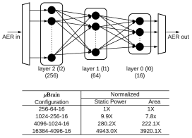
(a) 3-layered $\mu$Brain architecture.

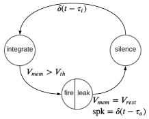
(b) State diagram of an IF neuron.

Figure 1: $\mu$Brain architecture and neuron state diagram [2].

$\mu$Brain can be scaled up to implement larger network topologies. However, static power and design area increases substantially for larger configurations as reported in Figure 1a. To improve energy efficiency, we propose a scalable many-core design where each core is a tiny-scale $\mu$Brain (see Section III).

II-B Other Neuromorphic Hardware Designs

Table I shows the capacity of recent neuromorphic designs. Here, we review two representative designs – DYNAPs and Loihi, and show that the proposed SentryOS framework can be easily extended to map SDCNN applications on them.

TABLE I: Capacity of recent neuromorphic hardware platforms [12, 13, 14, 15, 16].

	ODIN	$\mathbf{\mu}$Brain	DYNAPs	BrainScaleS	SpiNNaker	Neurogrid	Loihi	TrueNorth
# Neurons/core	256	336	256	512	36K	65K	130K	1M
# Synapses/core	64K	38K	16K	128K	2.8M	8M	130M	256M
# Cores/chip	1	1	1	1	144	128	128	4096
# Chips/board	1	1	4	352	56	16	768	4096
# Neurons	256	336	1K	4M	2.5B	1M	100M	4B
# Synapses	64K	38K	65K	1B	200B	16B	100B	1T

DYNAPs [3] is a mixed-signal inference hardware with four neurosynaptic cores. Each core can map up to 256 neurons and 16K synaptic connections. Cores are interconnected using a hierarchical NoC with mesh routing. Weights of a fully-trained network (i.e., the inference) are programmed to the synaptic cells of the four cores. Once programmed, DYNAPs can perform inference on streaming data continuously. Each DYNAPs core uses a crossbar where neurons are organized into two layers. Synaptic memory is tightly integrated with neuron circuits as in $\mu$Brain. SpiNeMap [17] is used to map applications on DYNAPs.

Loihi [4] is a digital design of a many-core neuromorphic hardware consisting of 128 cores with mesh routing. A Loihi core can map up to 130K neurons and 130M synaptic connections. Unlike $\mu$Brain and DYNAPs, synaptic memory in Loihi is off-chip to the neuron circuitry, leading to higher data movements. The LAVA framework [18] is used to map applications on Loihi.

II-C System Software for Neuromorphic Hardware

Apart from SpiNeMap and LAVA, there are also other system software frameworks for spiking neuromorphic accelerators – neutram [19], neuroxplorer [20], pacman [21], and dfsynthesizer [22], among others [23, 24, 25, 26]. All these frameworks use graph partitioning technique to first partition an SDCNN into clusters and then place these clusters onto homogeneous neuromorphic cores connected in a mesh-based topology. They cannot be easily extended to hardware with different core capacities and interconnected using segmented bus interconnect.

III Many-Core $\mu$Brain Design

Figure 2 illustrates a high-level architecture of the proposed many-core big little $\mu$Brain platform template design, where big (B) and little (L) cores are interconnected using parallel bus lanes that are segmented using segmentation switches (S). An SDCNN application (specified using Nengo [27], PyCARL [28] or PyNN [29]) is admitted to this platform using the proposed SentryOS framework. A bus controller is used to map inter-core data communication to parallel segments.

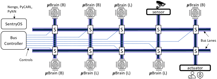
Figure 2: Many-core big little $\mu$Brain with dynamic segmented bus interconnect.

III-A Big Little $\mu$Brain Design

Figure 3 illustrates the structure of five commonly-used SDCNNs – LeNet (1989), AlexNet (2012), VGGNet (2015), ResNet (2015), and DenseNet (2017) [30]. We observe that LeNet, AlexNet, and VGGNet have a regular topology with chain-like connections. However, emerging CNNs such as ResNet (identity shortcut connections) and DenseNet (one-to-all subsequent layer connections) have an irregular topology [31]. Additionally for energy-efficient implementation on embedded devices, SDCNNs are subject to connection pruning, where connections with near-zero synaptic weights are removed [32]. Such pruning creates an irregular topology, even for LeNet, AlexNet, and VGGNet, making it difficult to map them onto hardware accelerators [33, 34, 35, 36, 37].

To this end, Table II reports the minimum, maximum, and average number of L1 and L2 neighbors of neurons from these five SDCNNs. We observe that the number of L1 and L2 neighbors of neurons in an SDCNN varies widely. To use $\mu$Brain for these models, the $\mu$Brain design needs to be optimally configured to accommodate the maximum number of L1 and L2 neighbors. This is reported as the conservative $\mu$Brain design choice in row 8 of Table II.

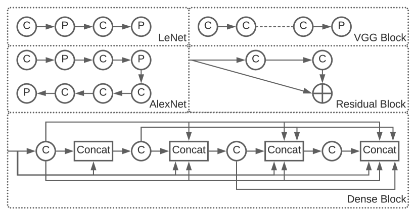
Figure 3: Structure of five commonly used CNNs with convolution (C), pooling (P), concatenation (concat), and addition (+) operations.

TABLE II: Statistics of CNN sub-networks [30].

	L1 neighbors			L2 neighbors
	Min	Max	Avg	Min	Max	Avg
LeNet	18	144	115.8	128	400	369.3
AlexNet	9	2566	41.9	11	10154	544.2
VGGNet	3	288	186.3	16	14772	2437.8
ResNet	12	288	244.9	16	1568	695.9
DenseNet	3	288	162.8	16	14772	1422.3
Conservative $\mu$Brain design	L1 neurons = 4,096			L2 neurons = 16,384

Figure 4 compares the average energy-per-core of the conservative design against a fully-custom design, where $\mu$Brain cores are configured based on the number of L1 and L2 neighbors of neurons for each SDCNN application. Energy numbers are normalized to the conservative design. We observe that the average energy-per-core of the fully-custom design is on average 36% lower than the conservative design. This is because the conservative design is sized based on the maximum number of l1 and l2 neighbors of a neuron. Such worst-case connectivity occurs only rarely in most applications and therefore, many synaptic connections remain unutilized. This leads to a high static power overhead. In Section V-D, we show that using only a few (e.g., 4) $\mu$Brain configurations, we can achieve similar energy efficiency as a fully-custom design.

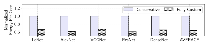
Figure 4: Average energy-per-core for five SDCNN applications.

III-B Segmented Bus Interconnect

Figure 5 illustrates the concept of a segmented bus-based many-core design (right) and its difference with a conventional bus (left) for interconnecting 7 $\mu$Brain cores ($\mathbf{C_{1}}$-$\mathbf{C_{7}}$). Let the core $\mathbf{C_{x}}$ has $\mathbf{M_{x}}$ input ports and $\mathbf{N_{x}}$ output ports. Without loss of generality, we consider a scenario where cores $\mathbf{C_{1}}$-$\mathbf{C_{4}}$ can only connect to the inputs of $\mathbf{C_{5}}$-$\mathbf{C_{7}}$. Fig. 5 (left) shows a single shared bus connecting $G=N_{1}+N_{2}+N_{3}+N_{4}$ output ports with $H=M_{5}+M_{6}+M_{7}$ input ports. While using shared bus, only one connection between any pair of input-output cluster is possible at a given time (shown with the arrow), resulting in underutilization of the bus. A simple segmented bus allows to overcome this problem by breaking the bus into multiple segments. As seen from Fig. 5 (right), a single segmented bus can accommodate many simultaneous connections.

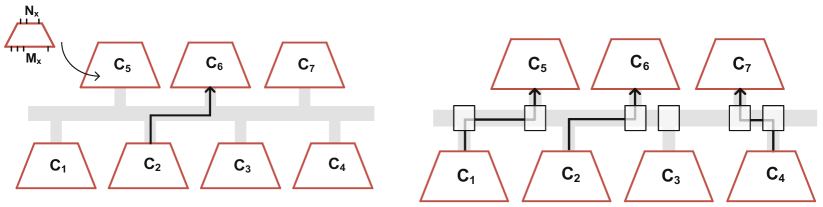
Figure 5: Segmented bus-based many-core design (right) and its difference with a conventional bus (left).

However, a single bus lane may not always be enough to support concurrent connection requests. For instance, any connection request from $\mathbf{C_{3}}$ to $\mathbf{C_{5}}$ will be blocked while $\mathbf{C_{2}}$ is communicating to $\mathbf{C_{6}}$. This can be solved using parallel bus lanes as illustrated in Figure 2. To achieve full connectivity at all time, $G*H$ separate busses are needed. However, such a full connection is rarely exercised in a typical SDCNN application. A more realistic scenario is the one where at different time intervals a different connection profile is active. We analyze inter-core communications based on training data to identify the minimum number of bus lanes needed in the parallel segmented bus interconnect at any given time. This minimum value is not dependent on the number of cores. The key idea here is to exploit the dynamism present in different SDCNN applications to virtualize the segmented bus interconnect between different cores. Hence, the bandwidth allocation needed at design-time can be reduced from the physical maximum to what is maximally happening concurrently. Consequently, the active wire length is reduced, which lowers energy. A bus controller is designed to control segmentation switches and map inter-core communications on parallel segments for concurrent execution. This reduces spike latency.

IV Detailed Design of SentryOS

We represent an SDCNN application as a graph. Formally,

Definition 1

(SDCNN Graph) An SDCNN application $\mathbf{G_{SDCNN}=(\mathbf{N},\mathbf{E})}$ is a directed graph consisting of a finite set ${\mathbf{N}}$ of nodes, representing neurons and a finite set ${\mathbf{E}}$ of edges, representing synaptic connections.

SentryOS consists of a compiler (SentryC) and a run-time manager (SentryRT) as illustrated in Figure 6.

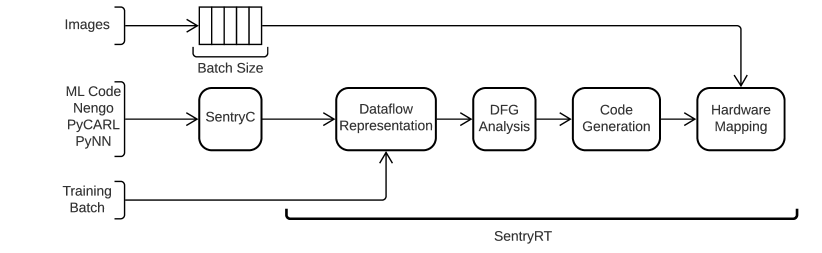
Figure 6: Detailed architecture of SentryRT.

IV-A Compiler (SentryC) Design

SentryC partitions the graph $G_{SDCNN}$ into sub-networks $\{S_{0},S_{1},\cdots\}$, where $S_{i}\bigcap S_{j}=\emptyset$. A sub-network $S_{i}=\{\texttt{l2}_{i}~{}|~{}\texttt{l1}_{i}~{}|\texttt{l0}_{i}\}$ is a set of neurons that are organized into three layers – l2, l1, and l0. $Area(S_{i})$ is the area of the $\mu$Brain core needed to implement $S_{i}$ and $Power(S_{i})$ is its static power. Algorithm 1 shows the pseudo-code of SentryC.

The algorithm operates in four steps. First, for each output neuron, we assign a distance value to all other neurons, where the distance is computed as the longest path from a neuron to this output neuron. Neurons that are not connected to this output neuron are assigned a large number (to prevent them from grouping in the same sub-network). Neurons with the same distance are clustered together as shown in Figure 7a. Second, we index each neuron by the distance sequence as shown in Figure 7b and form a search path for partitioning the graph into sub-networks: each sub-network must contain neurons with contiguous indexes. In this manner, any arbitrary network topology is transformed into a linear one.

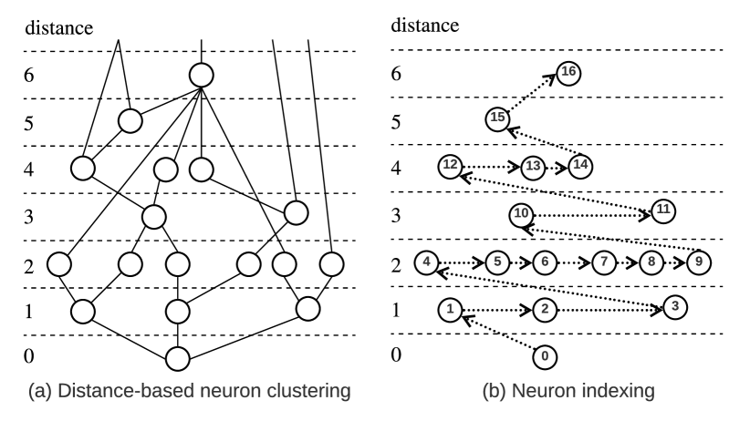
Figure 7: Distance-based partitioning an SDCNN application into subnetworks.

Third, we cluster neurons with distance of up to 2 into a sub-network, i.e., $S_{0}=\{N_{j}~{}|~{}dist(N_{j})\leq 2\}$. This is to ensure that each sub-network can fit into the three-layered architecture of $\mu$Brain. We compute the remaining graph as $G^{\prime}=G-\{S_{0}\}$. Next, we recursively partition the remaining graph $G^{\prime}$ for each node with distance 2 as the new output neuron and compute distance of all other neurons in $G^{\prime}$ by traversing backward.

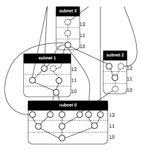
(a) Four sub-networks of the SDCNN example of Figure 7.

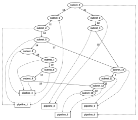
(b) Scheduling sub-networks to $\mu$Brain pipelines.

Figure 8: (a) Generating sub-networks by exploiting area-power benefits and (b) scheduling sub-networks of an SDCNN application to $\mu$Brain pipelines by exploiting data-level parallelism.

Figure 8a shows the four sub-networks of the SDCNN application of Figure 7. In generating a sub-network, it may be necessary to create neurons with unit synaptic strength in order to fit onto the three-layer architecture of $\mu$Brain. This is shown with the dotted neurons and connections inside sub-networks 1, 2, and 3.

Finally, we merge sub-networks (lines 7-12 of Algorithm 1) by considering area and power benefits of big and little $\mu$Brain cores. We formulate this problem as follows. Let $S_{i}$ and $S_{j}$ be two sub-networks of an SDCNN application. Formally, the merged sub-network is represented as $S_{i,j}=\{S_{i,j}.\texttt{l2}~{}|~{}S_{i,j}.\texttt{l1}~{}|~{}S_{i,j}.\texttt{l0}\}$, where $S_{i,j}.\texttt{l2}=\{S_{i}.\texttt{l2}\cup S_{j}.\texttt{l2}\}$, and so on. We merge $S_{i}$ and $S_{j}$ iff

• ${Area(S_{i,j})}<{Area(S_{i})}+{Area(S_{j})}$

• ${Power(S_{i,j})}<{Power(S_{i})}+{Power(S_{j})}$

IV-B Extension of SentryC to Other Spiking Architectures

IV-B1 Extension to DYNAPs

DYNAPs is a crossbar-based two-layer architecture with fixed number of l0 and l1 neurons. To use SentryC for DYNAPs, we make the following changes. First, we construct sub-networks with neurons that are at a distance 0 (layer 0) and 1 (layer 1) only, with a constraint on the size of a crossbar. This is accomplished by changing line 6 of Algorithm 1 to $S_{i}=\texttt{create\_subnet}\left(\underset{d(n_{j})\leq 1}{\bigcup}n_{j}\text{ such that }|S_{i}|\leq C_{n}\right)$, where $C_{n}$ is the total number of neurons that a crossbar can map. Second, we place all neurons that are at a distance of 2 or higher as candidates for sub-network generation in the next iteration. To do so, we change line 14 to $newNS.append(\underset{d(n_{j})=2}{\bigcup}n_{j})$. Finally, we assign all unassigned neurons from the current iteration and the new candidates to the list $NS$ for the next iteration of the algorithm, i.e., change line 16 to $NS=\{NS\setminus G^{\prime}\}\bigcup newNS$.

IV-B2 Extension to Loihi

To use SentryRT for Loihi, where neuron circuitry is decoupled from synaptic memory, we propose the same changes as DYNAPs with two constraints – one on the number of neurons and the other on the size of synaptic memory. Additionally, while placing a sub-network to a core, we decouple the neurons from the synapses and place them separately onto the target core architecture.

Input: $G_{SDCNN}=(\textbf{N},\textbf{E})$

Output: $G_{DFG}=(\textbf{S},\textbf{C})$

$G^{\prime}=G_{SDCNN}$;

  /* Initialize $G^{\prime}$ */

$NS=\{\underset{\texttt{OutDegree}(n_{i})=0}{\bigcup}n_{i}\}$;

  /* Place all output neurons. */

1 while $G^{\prime}\neq\emptyset$ do /* Run until all neurons of the graph are placed into sub-networks */

2       for $n_{i}\in NS$ do /* For each neurons in $NS$ */

             $d(n_{j})=\texttt{longest\_path}(n_{j},n_{i})~{}~{}\forall~{}n_{j}\in G^{\prime}$;

              /* Compute distance of every neuron in $G^{\prime}$ to $n_{i}$ */

             $S_{i}=\texttt{create\_subnet}\left(\underset{d(n_{j})\leq 2}{\bigcup}n_{j}\right)$;

              /* Create subnet with all neurons that have a distance of 2 or less from the output neuron */

3            

            Find $S_{j}~{}|~{}j=\texttt{argmin}\{Cost(S_{k},S_{i})~{}\forall~{}S_{k}\in G_{DFG}\}$;

              /* Find one subnet amongst the created ones to which merging this new subnet results in the minimum cost. Cost can be assessed in terms of area, power, or a combination of the two, which we have used in this paper. */

4             if $Area(S_{i,j})<Area(S_{i})+Area(S_{j})$ and $Power(S_{i,j})<Power(S_{i})+Power(S_{j})$ then /* If the area and power costs of merging the subnets is less than the individual costs. */

                   $S_{j}=S_{j}\bigcup S_{i}$;

                    /* Merge the subnets. */

5                  

6             else

                   $G_{DFG}.\texttt{append}(S_{i})$;

                    /* Insert this subnet to the output DFG */

7                  

8             end if

            $G^{\prime}=G^{\prime}-S_{i}$;

              /* Remove $S_{i}$ from $G^{\prime}$ */

             $newNS.append(\underset{d(n_{j})=3}{\bigcup}n_{j})$;

              /* Use the set $newNS$ to hold all neurons that are at a distance of 3. Neurons in this set will be placed in the next iteration. */

9            

10       end for

      $NS=newNS$;

        /* Update $NS$ to $newNS$. */

11      

12 end while

Algorithm 1 Compiler (SentryRT) of SentryOS.

IV-C Run-time Manager (SentryRT) Design

Figure 6 shows the proposed SentryRT. It queues input images to a given batch size and process them concurrently. Although queuing increases latency, the throughput is higher due to batch processing. SentryRT uses a dataflow analysis technique to schedule sub-networks onto $\mu$Brain cores to improve throughput. To this end, SentryRT uses a training batch to profile an SDCNN application and represent its sub-networks and their interconnections as a dataflow graph (DFG). Formally,

Definition 2

(SDCNN DFG Graph) An SDCNN dataflow graph $\mathbf{G_{DFG}=(\mathbf{S},\mathbf{C})}$ is a directed graph consisting of a finite set ${\mathbf{S}}$ of sub-networks of the SDCNN application and a finite set ${\mathbf{C}}$ of communication channels between the sub-networks.

Each sub-network $S_{i}\in\mathbf{S}$ is associated with an execution time $t_{i}$, which represents its computation time on a $\mu$Brain core.

SentryRT uses an analytical approach to timing analysis of $G_{DFG}$ [38]. It consists of a novel way of constructing a Max-Plus algebraic description of the evolution of node execution times in a self-timed execution manner. The Max-Plus semiring $\mathbb{R}_{\text{max}}$ is the set $\mathbb{R}\cup\{-\infty\}$ defined with two basic operations $\oplus\text{ and }\otimes$, which are related to linear algebra as $a\oplus b=\max(a,b)\text{ and }a\otimes b=a+b$. The identity element $\mymathbb{0}$ for the addition $\oplus$ is $-\infty$ in linear algebra, i.e., $a\oplus\mymathbb{0}=a$. The identity element $\mymathbb{1}$ for the multiplication $\otimes$ is 0 in linear algebra, i.e., $a\otimes\mymathbb{1}=a$. The end execution time of each node of $G_{DFG}$ can be expressed as $\mathbf{t_{k}}=\oplus\mathbf{{T}\otimes t_{k-1}}$, where $\mathbf{{T}}$ captures execution times of sub-networks $\tau_{n}$ and $\mathbf{t_{k}}=\{t_{0}(k),t_{1}(k),\cdots\}$ is the end execution of nodes in the $k^{th}$ iteration. Figure 9a shows the schedule obtained by solving the Max-Plus formulation of end execution time of sub-networks of an SDCNN micro-benchmark shown in Figure 8b.

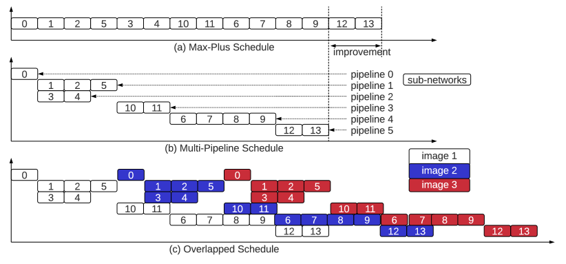
Figure 9: Schedule of sub-networks generated by SentryRT.

To exploit parallelism, SentryRT discards the precise execution time of sub-networks, retaining only their sequence. Sub-networks are executed in a self-timed fashion when data is available for its neurons to compute. Figure 8b shows the allocation of sub-networks to 6 $\mu$Brain pipelines, where each pipeline may consist of a few $\mu$Brain cores. The corresponding multi-pipeline schedule is illustrated in Figure 9b. Finally, SentryRT overlaps execution of pipelines for different images of a batch to improve throughput. Figure 9c shows this overlapped execution for three different input images.

V Evaluation

$\mu$Brain design is synthesized at 40 nm technology node using TSMC library CLN40LP. Area and power numbers for different $\mu$Brain configurations are estimated using the compact model provided in [2]. We use an in-house cycle-accurate neuromorphic platform simulator to simulate many-core $\mu$Brain cores interconnected using a segmented bus interconnect. We use PyCARL [28] to simulate five commonly-used SDCNN applications with 2-bit quantized synaptic weights. These applications are described in Table III.

TABLE III: SDCNN applications used to evaluate the proposed design.

SDCNN	Dataset	Neurons	Synapses	Avg. Spikes/Image	Accuracy
LeNet	CIFAR-10	80,271	275,110	724,565	86.3%
AlexNet	CIFAR-10	127,894	3,873,222	7,055,109	66.4%
VGGNet	CIFAR-10	448,484	22,215,209	12,826,673	81.4 %
ResNet	CIFAR-10	266,799	5,391,616	7,339,322	57.4%
DenseNet	CIFAR-10	365,200	11,198,470	1,250,976	46.3%

V-A Energy Efficiency

Figure 10 plots the core energy of DYNAPs, Loihi, and the proposed many-core $\mu$Brain design for all five SDCNN applications. We scale DYNAPs and Loihi to 40nm node (the same technology node as $\mu$Brain). We use the proposed SentryOS for all these three spiking neuromorphic accelerators. Results are normalized to DYNAPs. We make two key observations.

Figure 10: Core energy normalized to DYNAPs.

First, energy of Loihi is on average 5% lower than DYNAPs. Although Loihi requires higher energy to access off-chip synaptic memory, the improvement is due to larger capacity of a Loihi core compared to DYNAPs. For smaller applications like LeNet, energy numbers are comparable. Second, energy using the proposed design is on average 32% lower than DYNAPs and 29% lower than Loihi. This improvement is because 1) a $\mu$Brain core consumes lower power than a DYNAPs and Loihi core [2], 2) contrary to DYNAPs and Loihi, the proposed design uses different capacity (big little) $\mu$Brain cores, which significantly reduces unused synaptic connections and improves energy efficiency, 3) the proposed design uses parallel segmented bus interconnect, which is more energy efficient than a traditional mesh-based NoC, which is used in DYNAPs and Loihi, and 4) contrary to Loihi, where synaptic memory is separated from neurons, $\mu$Brain requires very low data movement because of the integration of synaptic memory with neurons.

V-B Throughput

Figure 11 plots throughput of the evaluated SDCNN applications on the proposed design. We compare SentryOS with a previously-proposed framework SpiNeMap. Results are normalized to SpiNeMap. We make two observations.

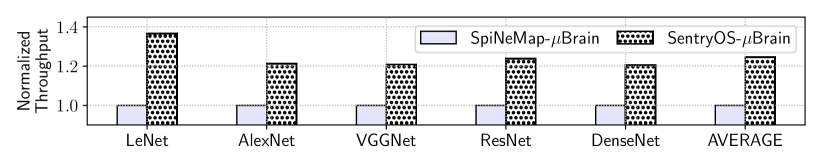
Figure 11: Throughput normalized to SpiNeMap.

First, throughput using SentryOS is on average 25% higher than SpiNeMap. This improvement is because, SentryOS first compiles an SDCNN into sub-networks by exploiting the internal architecture of big and little $\mu$Brain cores and then uses a dataflow analysis technique to schedule sub-networks to cores improving opportunities for pipelining and exploiting data-level parallelism. Second, even for irregular topologies such as ResNet and DenseNet, SentryOS results in an average 22% higher throughput than SpiNeMap.

V-C $\mu$Brain Design Choice: Segmented Bus Interconnect

Figure 12 plots interconnect energy and latency of the proposed many-core design with segmented bus (SB) compared to a mesh-based network-on-chip (NoC) interconnect. We make the following two key observations.

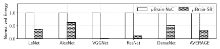
(a) Normalized interconnect energy.

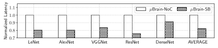
(b) Normalized latency.

Figure 12: Comparing $\mu$Brain design with segmented bus (SB) interconnect to mesh-based network-on-chip (NoC) interconnect.

First, energy using segmented bus interconnect is on average 67% lower than NoC. This improvement is because 1) we analyze inter-core communication based on training data to identify the minimum number of parallel bus lanes needed in the segmented bus interconnect, which reduces the active wire length compared to NoC, and 2) core-to-core communications do not need to wake and utilize the entire bus; rather, only segments connecting the communicating cores need to be powered up. Second, latency using segmented bus is on average 18% lower than that of NoC. This is because in the proposed design, segmentation switches are programmed once at design-time before admitting an application. This is done by analyzing the communication profile. Since there is no run-time routing decisions involved, latency is lower.

V-D $\mu$Brain Design Choice: Heterogeneous Configurations

Figure 13 plots energy of the proposed $\mu$Brain-based many-core design with 1, 2, 4, and 8 different $\mu$Brain configurations. The proposed design with a single configuration is the conservative design of Table II. All results are normalized to this conservative design. We make two observations.

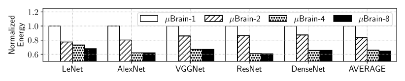
Figure 13: Energy for different $\mu$Brain configurations.

First, with 2, 4, and 8 configurations, energy is on average 16%, 35%, and 36% lower than the conservative design, respectively. In comparison, energy of a fully-custom SDCNN-specific design, where cores can be of difference sizes, is 36% lower than the conservative design (see Fig. 4). Energy reduces with more configurations due to the reduction of unused synaptic connections in each core. Second, increasing from 4 to 8 configurations, the reduction of energy is less than 1%. In our proposed design template, we have used only four configurations – 1) little, type 1 $(256\times 64\times 16)$, 2) little, type 2 $(1024\times 256\times 16)$, 3) big, type 1 $(4096\times 1024\times 16)$, and 4) big. type 2 $(16384\times 4096\times 16)$, instead of adopting a fully-custom SDCNN-specific design. This is to make the design generic and applicable to many different SDCNN inference applications.

VI Conclusion

We introduce a many-core neuromorphic platform template consisting of asynchronous (clock-less) big little digital $\mu$Brain cores interconnected using a segmented bus interconnect. We propose a system software framework SentryOS, consisting of a compiler and a run-time manager, to compile spiking deep convolutional neural network (SDCNN) to the proposed design. Using five commonly-used SDCNN applications, we show a significant improvement in energy, latency, and throughput.

References

- [1] Y. Cao et al., “Spiking deep convolutional neural networks for energy-efficient object recognition,” IJCV, 2015.
- [2] J. Stuijt et al., “Brain: An event-driven and fully synthesizable architecture for spiking neural networks,” Frontiers in Neuroscience, 2021.
- [3] S. Moradi et al., “A scalable multicore architecture with heterogeneous memory structures for dynamic neuromorphic asynchronous processors (DYNAPs),” TBCAS, 2017.
- [4] M. Davies et al., “Loihi: A neuromorphic manycore processor with on-chip learning,” IEEE Micro, 2018.
- [5] Y. S. Yang et al., “Recent trend of neuromorphic computing hardware: Intel’s neuromorphic system perspective,” in ISOCC, 2020.
- [6] S. A. Wasif et al., “Energy efficient synchronous-asynchronous circuit-switched NoC,” in MOCAST, 2020.
- [7] X. Liu et al., “Neu-NoC: A high-efficient interconnection network for accelerated neuromorphic systems,” in ASP-DAC, 2018.
- [8] Y. J. Yoon et al., “System-level design of networks-on-chip for heterogeneous systems-on-chip,” in NOCS, 2017.
- [9] A. Balaji et al., “Exploration of segmented bus as scalable global interconnect for neuromorphic computing,” in GLSVLSI, 2019.
- [10] J. Chen et al., “Segmented bus design for low-power systems,” TVLSI, 1999.
- [11] S. Fusi et al., “Collective behavior of networks with linear (VLSI) integrate-and-fire neurons,” Neural Computation, 1999.
- [12] H. Benmeziane et al., “Hardware-aware neural architecture search: Survey and taxonomy,” in IJCAI, 2021.
- [13] K. J. Lee et al., “The development of silicon for AI: Different design approaches,” TCAS I: Regular Papers, 2020.
- [14] C. D. Schuman et al., “A survey of neuromorphic computing and neural networks in hardware,” arXiv preprint arXiv:1705.06963, 2017.
- [15] F. Catthoor et al., “Very large-scale neuromorphic systems for biological signal processing,” in CMOS Circuits for Biological Sensing and Processing, 2018.
- [16] A. Paul et al., “Design technology co-optimization for neuromorphic computing,” in IGSC Workshops, 2021.
- [17] A. Balaji et al., “Mapping spiking neural networks to neuromorphic hardware,” TVLSI, 2020.
- [18] C.-K. Lin et al., “Mapping spiking neural networks onto a manycore neuromorphic architecture,” in PLDI, 2018.
- [19] Y. Ji et al., “NEUTRAMS: Neural network transformation and co-design under neuromorphic hardware constraints,” in MICRO, 2016.
- [20] A. Balaji et al., “NeuroXplorer 1.0: An extensible framework for architectural exploration with spiking neural networks,” in ICONS, 2021.
- [21] F. Galluppi et al., “A hierachical configuration system for a massively parallel neural hardware platform,” in CF, 2012.
- [22] S. Song et al., “DFSynthesizer: Dataflow-based synthesis of spiking neural networks to neuromorphic hardware,” TECS, 2021.
- [23] T. Titirsha et al., “Endurance-aware mapping of spiking neural networks to neuromorphic hardware,” TPDS, 2021.
- [24] T. Titirsha et al., “On the role of system software in energy management of neuromorphic computing,” in CF, 2021.
- [25] S. Song et al., “Dynamic reliability management in neuromorphic computing,” JETC, 2021.
- [26] A. Amir et al., “Cognitive computing programming paradigm: a corelet language for composing networks of neurosynaptic cores,” in IJCNN, 2013.
- [27] T. Bekolay et al., “Nengo: a python tool for building large-scale functional brain models,” Frontiers in Neuroinformatics, 2014.
- [28] A. Balaji et al., “PyCARL: A PyNN interface for hardware-software co-simulation of spiking neural network,” in IJCNN, 2020.
- [29] A. P. Davison et al., “PyNN: a common interface for neuronal network simulators,” Frontiers in Neuroinformatics, 2009.
- [30] A. Sengupta et al., “Going deeper in spiking neural networks: VGG and residual architectures,” Frontiers in Neuroscience, 2019.
- [31] S. Zheng et al., “Efficient scheduling of irregular network structures on CNN accelerators,” TCAD, 2020.
- [32] T. Augustine et al., “Generating piecewise-regular code from irregular structures,” in PLDI, 2019.
- [33] N. Voss et al., “Convolutional neural networks on dataflow engines,” in ICCD, 2017.
- [34] J. Shan et al., “Exact and heuristic allocation of multi-kernel applications to multi-FPGA platforms,” in DAC, 2019.
- [35] P. Xu et al., “AutoDNNchip: An automated DNN chip predictor and builder for both FPGAs and ASICs,” in FPGA, 2020.
- [36] S. Song et al., “A design flow for mapping spiking neural networks to many-core neuromorphic hardware,” in ICCAD, 2021.
- [37] S. Curzel et al., “Automated generation of integrated digital and spiking neuromorphic machine learning accelerators,” in ICCAD, 2021.
- [38] L. Thiele et al., “Real-time calculus for scheduling hard real-time systems,” in ISCAS, 2000.