Harmless Sets in Sparse Classes

Abstract

In the classic Target Set Selection problem, we are asked to minimise the number of nodes to activate so that, after the application of a certain propagation process, all nodes of the graph are active. Bazgan and Chopin [Discrete Optimization, 14:170–182, 2014] introduced the opposite problem, named Harmless Set, in which they ask to maximise the number of nodes to activate such that not a single additional node is activated.

In this paper we investigate how sparsity impacts the tractability of Harmless Set. Specifically, we answer two open questions posed by the aforementioned authors, namely a) whether the problem is on planar graphs and b) whether it is parametrised by treewidth. The first question can be answered in the positive using existing meta-theorems on sparse classes, and we further show that Harmless Set not only admits a polynomial kernel, but that it can be solved in subexponential time. We then answer the second question in the negative by showing that the problem is W[1]-hard when parametrised by a parameter that upper bounds treewidth.

1 Introduction

How information and cascading events spread through social and complex networks is an important measure of their underlying systems, and is a well-researched area in network science. The dynamic processes governing the diffusion of information and “word-of-mouth” effects have been studied in many fields, including epidemiology, sociology, economics, and computer science [21, 22, 16, 3].

A classic propagation problem is the Target Set Selection problem, first studied by Domingos and Richardson [12, 31], and later formalised in the context of graph theory by Chen [3, 6]. Chen defines the problem as how to find $k$ initial seed vertices that when activated cascade to a maximum; this model is called standard independent cascade model of network diffusion. It has also been studied under the name of Influence Maximization [28, 27] in the context of lies spreading through a network [4, 5], bio-terrorism [14], and the spread of fires [32]. Information propagation is modelled as an activation process where each individual is activated if a sufficient number of its neighbours are active. Sufficient here means that the number of active neighbours of an individual $v$ exceeds a given threshold $t(v)$ which is assigned to each individual to capture their resilience to being influenced.

Motivated by cascading of information we study vertices that are harmless, i.e., a set of vertices that can be activated without any cascades whatsoever. However, activating all vertices in a graph is a trivial solution in the standard diffusion model, since we cannot cascade further. We therefore want to differentiate between initially activated vertices and vertices that have been activated by a cascade. In this setting, we can therefore say that we want a largest possible set of initially activated vertices that do not cascade at all, even to itself. It was first studied by Bazgan and Chopin [1] under the name Harmless Set, who showed that it is [2]-complete in general and [1]-complete if thresholds are bounded by a constant. They observe (see Observation 1 below) that one can bound the maximum threshold by the solution size and thus obtain a simple algorithm when parametrised by the solution size $k$ and the treewidth. Bazgan and Chopin conclude their work with the following open questions:

Open question (Bazgan and Chopin [1]).

Is Harmless Set fixed-parameter tractable on

1. general graphs with respect to the parameter treewidth?

2. on planar graphs with respect to the solution size?

Here we answer both these problems: no and yes, and simultaneously discover surprising connections between Harmless Set and Dominating Set in sparse graphs.

Our results.

Let us distinguish two flavours of this problem: $p$-Bounded Harmless Set, where we consider the bound $p$ a constant, and Harmless Set where the threshold is unbounded.

Note that harmless sets are hereditary in the sense that if $S$ is a harmless set of an instance $(G,t)$, then any subset $S^{\prime}\subseteq S$ is also harmless for $(G,t)$. Therefore instead of searching for a harmless set of size at least $k$, we can equivalently search for a harmless set of size exactly $k$. In this scenario we can replace all thresholds above $k$ with $k+1$:

Observation 1.

Harmless Set parametrised by $k$ is equivalent to $(k+1)$-Bounded Harmless Set parametrised by $k$.

Let us begin by briefly answering the first question of Bazgan and Chopin in the positive. It turns out that a simple of application the powerful machinery of first-order model checking in sparse classes [20] is enough (see Appendix for a short proof):

Proposition 1 ().

Harmless Set parametrised by $k$ is fixed-parameter tractable in nowhere dense classes.

We will briefly discuss the notion of nowhere denseness below, in this context it is only important that planar graphs are nowhere dense.

These previous results and our observation regarding tractability in sparse classes leave two important questions for us. First, does the problem admit a polynomial kernel in sparse classes? And second, is there a chance that the problem could be solved on graphs of bounded treewidth without parametrising by the solution size? In the following we answer the kernelization question in the affirmative:

Theorem 1.1.

Harmless Set admits a polynomial sparse kernel in classes of bounded expansion. $p$-Bounded Harmless Set, for any constant $p$, admits a linear sparse kernel in these classes.

Classes with bounded expansion include planar graphs (and generally graphs of bounded genus), graphs of bounded degree, classes excluding a (topological) minor, and more. The term sparse kernel is explained below in Section 2.1; It alludes to the fact that the constructed kernel does not necessarily belong to the original graph class but is guaranteed to be “almost” as sparse.

Bazgan and Chopin give an algorithm for Harmless set parametrised by treewidth and the solution size running in time $O(k^{O(\text{tw})}\cdot n)$, when provided a tree decomposition as part of the input. They conclude by asking whether the problem is “fixed-parameter tractable on general graphs with respect to the parameter treewidth [alone]” [1]. We answer this question in the negative:

Theorem 1.2 ().

Harmless Set is [1]-hard when parametrised by a modulator to a $2$-spider-forest.

Since a $2$-spider-forest has treedepth, pathwidth, and treewidth at most 3, a graph with a modulator $M$ to a $2$-spider-forest has treedepth, pathwidth, and treewidth at most $|M|+3$. This very strong structural parametrisation means that the problem is not only hard on general sparse graphs, but indeed also [1]-hard for parameters like treewidth, pathwidth, and even treedepth. We complement this result by showing that a slightly stronger parameter, the vertex cover number, does indeed make the problem tractable:

Theorem 1.3 ().

Harmless Set is fixed-parameter tractable when parametrised by the vertex cover number of the input graph.

Note.

We obtained our results simultaneously with and independent from those by Gaikwad and Maity [19]. They provide an explicit and potentially practical FPT algorithm for planar graphs while we show that the problem is not only FPT on planar graphs, but indeed on a much more general class of graphs, namely those of bounded expansion. We also show that on apex-minor-free graphs (which include planar graphs), there exists a subexponential time algorithm for the problem. That is, we show the following results, which improves on Gaikwad and Maity’s $2^{O(k\log k)}n^{O(1)}$ algorithm for planar graphs:

Theorem 1.4 ().

Harmless Set is solvable in time $O(2^{o(k)}\cdot n)$ on apex-minor-free graphs.

2 Preliminaries

For a graph $G$ we use $V(G)$ and $E(G)$ to refer to its vertex- and edge-set, respectively. We used the short hands $|G|:=|V(G)|$ and $\|G\|:=|E(G)|$. A $2$-spider is a graph obtained from a star by subdividing every edge at most once. A $2$-spider-forest is the disjoint union of arbitrarily many $2$-spiders.

For functions $f\colon V(G)\to\mathbb{R}$ we will often use the shorthands $f(X):=\sum_{u\in X}f(x)$ and $f(G):=f(V(G))$. Similarly, we use the shorthand $N(X):=(\bigcup_{u\in X}N(u))\setminus X$ for all neighbours of a vertex set $X$. The $r$^th neighbourhood $N^{r}(u)$ contains all vertices at distance exactly $r$ from $u$, the closed $r$^th neighbourhood $N^{r}[u]$ all vertices at distance at most $r$ from $u$ (also known as the $r$-ball of $u$). This corresponds to $N(u)=N^{1}(u)$ and $N[u]=N^{1}[u]$. We refer to the textbook by Diestel [11] for more on graph theory notation.

A vertex set $X\subseteq V(G)$ is $r$-scattered if for $x_{1}\in X$ and $x_{2}\in X$, $N^{r}[x_{1}]\cap N^{r}[x_{2}]=\varnothing$. Equivalently, $N^{r}[u]\cap X\leqslant 1$ for all vertices $u\in G$, or the pairwise distance between members of $X$ is at least $2r+1$. A vertex set $D\subseteq V(G)$ is $r$-dominating if $N^{r}[D]=V(G)$ and we write $\operatorname{\mathbf{dom}}_{r}(G)$ to denote the minimum size of such a set. Similarly, we say that $D$ $r$-dominates another vertex set $X\subseteq V(G)$ if $X\subseteq N^{r}[D]$ and we write $\operatorname{\mathbf{dom}}_{r}(G,X)$ for the minimum size of such a set. In both cases we will omit the subscript $r$ for the case of $r=1$. In classes with bounded expansion, the size of $r$-scattered sets is closely related to the $r$-domination number, see the toolkit section below.

Given a vertex set $X\subseteq V(G)$ we call a path $X$-avoiding if its internal vertices are not contained in $X$. A shortest $X$-avoiding path between vertices $x,y$ is shortest among all $X$-avoiding paths between $x$ and $y$.

Definition 1 ($r$-projection).

For a vertex set $X\subseteq V(G)$ and a vertex $u\not\in X$ we define the $r$-projection of $u$ onto $X$ as the set

$$P^{r}_{X}(u):=\{v\in X\mid\text{there exists an $X$-avoiding $u$-$v$-path of length}\leqslant r\}\vspace*{-6pt}$$

Two vertices with the same $r$-projection onto $X$ do not, however, necessarily have the same (short) distances to $X$. To distinguish such cases, it is useful to consider the projection profile of a vertex to its projection:

Definition 2 ($r$-projection profile).

For a vertex set $X\subseteq V(G)$ and a vertex $u\not\in X$ we define the $r$-projection profile of $u$ onto $X$ as a function $\pi^{r}_{G,X}[u]\colon X\to[r]\cup\infty$ where $\pi^{r}_{G,X}[u](v)$ for $v\in X$ is the length of a shortest $X$-avoiding path from $u$ to $v$ if such a path of length at most $r$ exists and $\infty$ otherwise.

2.1 Bounded expansion classes and kernels

Nešetřil and Ossona de Mendez [26] introduced bounded expansion as a generalisation of many well-known sparse classes like planar graphs, graphs of bounded genus, bounded-degree graphs, classes excluding a (topological) minor, and more. The original definition of bounded expansion classes made use of the concept of shallow minors inspired by the work of Plotkin, Rao, and Smith [29].

Definition 3.

A graph $H$ is an $r$-shallow minor of $G$, written as $H\preccurlyeq_{\mathrlap{\mathsf{m}}}^{r}G$, if $H$ can be obtained from $G$ by contracting disjoint sets of radius at most $r$.

Classes of bounded expansion are then defined as those classes in which the density (or average degree) of $r$-shallow minors is bounded by a function of $r$.

Definition 4.

The greatest-reduced average degree (grad) $\nabla\!_{r}$ of a graph $G$ is defined as

$$\nabla\!_{r}(G)=\sup_{H\preccurlyeq_{\mathrlap{\mathsf{m}}}^{r}G}\frac{\|H\|}{|H|}$$

Definition 5.

A graph class $\mathcal{G}$ has bounded expansion if there exists a function $f$ such that $\nabla\!_{r}(G)\leqslant f(r)$ for all $G\in\mathcal{G}$.

For example, it is easy to see that classes with maximum degree $\Delta$ have bounded expansion with $f(r):=\Delta^{r+1}$. In the following we will often make use of the property that the grad of a graph does not change much under the addition of a few high-degree vertices: if $G$ is a graph and $G^{\prime}$ is obtained from $G$ by adding an apex-vertex, then $\nabla\!_{r}(G^{\prime})\leqslant\nabla\!_{r}(G)+1$.

One principal issue with designing kernels for bounded expansion classes is the uncertainty of whether certain gadget constructions preserve the class or not. When working with more concrete classes like planar graphs we can be certain that adding pendant vertices will result in a planar graph. When working with some arbitrary bounded expansion class $\mathcal{G}$ this is not necessarily possible: $\mathcal{G}$ might, for example, consist of all graphs with grad bounded by some function and minimum degree at least two. In such cases, the addition of a pendant vertex takes us outside of the class even though the grad did not increase.

We resolve this issue as proposed in the paper [17]. Let $\Pi$ be a parametrised problem over graphs. A sparse kernel of $\Pi$ is a kernelization for which there exists a function $g$ that, given an instance with graph $G$, outputs a graph $G^{\prime}$ that besides the usual constraints on the size $|G|+\|G^{\prime}\|$ further satisfies that $\nabla\!_{r}(G^{\prime})\leqslant g(\nabla\!_{r}(G))$ for all $r\in\mathbb{N}$. Therefore if the input graphs are taken from a bounded expansion class $\mathcal{G}$, the outputs will also belong to a, potentially different, bounded expansion class $\mathcal{G}^{\prime}$.

2.2 The bounded expansion toolkit

The notion of independence (or more specifically scatteredness) plays a central role in the theory of sparse graphs. As a prime example, Dawar [8, 9] introduced the notions of wideness and quasi-wideness—both related to independence—as one possible classification of sparseness. We will need the following definition from his work; recall that an $r$-scattered set is a set of vertices $X\subseteq V(G)$ such that for any vertex $u$ in $V(G)$, the $r$-ball of $u$ contains at most 1 vertex from $X$.

Definition 6.

A class $\mathcal{G}$ is uniformly quasi-wide if for every $m\in\mathbb{N}$ and $r\in\mathbb{N}$ there exist numbers $N=N(m,r)$ and $s=s(r)$ such that the following holds:

Let $G\in\mathcal{G}$ and let $A\subseteq V(G)$ with $|A|\geqslant N$. Then there exists $S\subseteq V(G)$, $|S|\leqslant s(r)$ and a set $B\subseteq A-S$, $|B|\geqslant m$, such that $B$ is $r$-scattered in $G-S$.

As it turns out this notion of sparseness coincides with the notion of nowhere denseness in graph classes closed under taking subgraphs [25]. Bounded expansion classes are nowhere dense and the following result due to Kreutzer, Rabinovich, and Siebertz plays a crucial role in our kernelization procedure.

Theorem 2.1 (Kreutzer, Rabinovich, Siebertz [23]).

Every nowhere dense class $\mathcal{G}$ is uniformly quasi-wide with $N(m,r)=m^{g(r)}$ for some function $g$. Moreover, there exists an algorithm which, given $G\in\mathcal{G}$ and $A\subseteq V(G)$ as input, computes an $r$-scattered set of the promised size in time $|A|^{O(1)}n^{1+o(1)}$.

There is a second method to compute suitable scattered sets which we can leverage to create a “win-win” argument for our kernelization procedure. Concretely, Dvořák’s algorithm [15] provides us either with a small $r$-dominating set or a large $r$-scattered set. The following variant of the original algorithm is called the warm-start variant (see [17]):

Theorem 2.2 (Dvořák’s algorithm [15]).

For every bounded expansion class $\mathcal{G}$ and $r\in\mathbb{N}$ there exists a polynomial-time algorithm that, given a vertex set $X\subseteq V(G)$, computes an $r$-dominating set $D$ of $X$ and an $r$-scattered set $I\subseteq D\cap X$ with $|D|=O(|I|)$.

Note that since an $r$-scattered set $I\subseteq X$ provides a lower bound for the $r$-domination of $X$ we have that $|D|=O(\operatorname{\mathbf{dom}}_{r}(G,X))$.

Finally, we will need the following two fundamental properties of bounded expansion classes. The first is a refinement on the neighbourhood complexity characterisation of bounded expansion classes [30]:

Lemma 1 (Adapted from [13, 23]).

For every bounded expansion class $\mathcal{G}$ and $r\in\mathbb{N}$ there exists a constant $\mathsf{c}^{\text{proj}}_{r}$ such that for every $G\in\mathcal{G}$ and $X\subseteq V(G)$, the number of $r$-projection profiles realised on $X$ is at most $\mathsf{c}^{\text{proj}}_{r}|X|$.

The second can be seen as a strengthening of the first: not only are the number of projection profiles bounded linearly in the size of the target set, we can find a suitable superset of the target set which even restricts the size of the projections to a constant.

Lemma 2 (Projection closure [13]).

For every bounded expansion class $\mathcal{G}$ and $r\in\mathbb{N}$ there a polynomial-time algorithm that, given $G\in\mathcal{G}$ and $X\subseteq V(G)$, computes a superset $X^{\prime}\supseteq X$, $|X^{\prime}|=O(|X|)$, such that $|P^{r}_{X^{\prime}}(u)|=O(1)$ for all $u\in V(G)\setminus X^{\prime}$.

2.3 Waterlilies

Reidl and Einarson introduced the notion of waterlilies as a structure which is very useful in constructing kernels [17]. We simplify the definition here as we do not need it in its full generality.

Definition 7 (Waterlily).

A waterlily of radius $r$ and depth $d\leqslant r$ in a graph $G$ is a pair $(R,C)$ of disjoint vertex sets with the following properties:

• $C$ is $r$-scattered in $G-R$,

• $N^{r}_{G-R}[C]$ is $d$-dominated by $R$ in $G$.

We call $R$ the roots, $C$ the centres, and the sets $\{N^{r}_{G-R}[x]\}_{x\in C}$ the pads of the waterlily. A waterlily is uniform if all centres have the same $d$-projection onto $R$, $\pi^{d}_{R}[x]$ is the same function for all $x\in C$.

We will frequently talk about the ratio of a waterlily which we define as a guaranteed lower bound of $|C|$ in terms of $|R|$, a waterlily of ratio $2|R|+1$ satisfies $|C|\geqslant 2|R|+1$. The authors in [17] used waterlilies with a constant ratio, but a slight modification of their proof (in particular using Theorem 2.1) lets us improve this ratio to any polynomial. We provide a proof with the necessary modification in the Appendix.

Lemma 3 ().

For every bounded expansion class $\mathcal{G}$ and $r,d\in\mathbb{N}$, $d\leqslant r$, the following holds. There exists a polynomial $p_{r}$ such that for every $G\in\mathcal{G}$, $t\in\mathbb{N}$ and $A\subseteq V(G)$ with $|A|\geqslant p_{r}(t)\operatorname{\mathbf{dom}}_{d}(G,A)$ there exists a uniform waterlily $(R,C\subseteq A)$ with depth $d$, radius $r$, and with $|R|=O(1)$ and $|C|\geqslant t$, moreover, such a waterlily can be computed in polynomial time.

3 A sparse kernel for $p$-Bounded Harmless Set

In order to give a sparse kernel we first show how to construct a bikernel into the following annotated problem.

We call the set $K$ the solution core of the instance (see [17] for a general definition). Next we present two lemmas whose application will step-wise construct smaller annotated instances. The first lemma lets us reduce the size of the solution core, the second the size of the graph. Afterwards we demonstrate how these two reduction rules serves to construct a bikernel.

In the following, we often need to treat vertices with a threshold equal to one differently. For brevity, we will call these vertices fragile; observe that a fragile vertex can be part of a solution but none of its neighbours can.

Lemma 4.

Let $(G,t,k,K)$ be an instance of Annotated $p$-Bounded Harmless Set where $G$ is taken from a bounded expansion class and $K$ is a solution core. There exists a polynomial $q(p)$ such that the following holds: If $|K|\geqslant q(p)\cdot k$, then in polynomial time we either find that $(G,t,k,K)$ is a YES-instance or we identify a vertex $x\in K$ such that $K\setminus\{x\}$ is a solution core.

Proof.

First consider the case that there is a vertex $x\in K$ with a fragile neighbour $u\in N(x)$. Then $x$ of course cannot be in any solution and $K\setminus\{x\}$ is a solution core.

Assume now that no vertex in $K$ has a fragile neighbour. We now use Dvořák’s algorithm (Theorem 2.2) to compute a $1$-dominating set for $K$; let $D$ be the resulting dominating set and $I\subseteq D\cap K$ the promised $1$-scattered set, i.e., with $|I|=\Omega(|D|)$. Since the neighbourhoods of vertices in $I$ are pairwise disjoint and no vertex in $I$ (as $I\subseteq K$) has a fragile neighbour, it follows that $I$ itself is a harmless set. So if $|I|\geqslant k$ we conclude that $(G,t,k,K)$ is a YES-instance.

Otherwise $|I|<k$ and therefore, by Theorem 2.2, $\operatorname{\mathbf{dom}}(G,K)=O(k)$. We apply Lemma 3 to compute a waterlily for the set $K$ at depth $1$ and with radius $2$. We will later choose $q(k)$ to ensure that the following arguments go through.

Let $(R,C\subseteq K)$ be the resulting uniform waterlily with $|C|\geqslant\kappa$, where $\kappa$ is an appropriately large value that we choose later. For the centres $v\in C$, define the following signature $\sigma(v)$:

$$\sigma(v)=\{(t(u),N(u)\cap R)\mid u\in N_{G-R}(v)\}.$$

That is, $\sigma(v)$ records how neighbours of $v$ connect to $R$ and what thresholds these neighbours have. Define the equivalence relation $\sim_{\sigma}$ over $C$ via $v\sim_{\sigma}w$ iff $\sigma(v)=\sigma(w)$. Recall that, by Lemma 1 the number of $1$-projections onto $R$ is at most $\mathsf{c}^{\text{proj}}_{1}|R|$. Therefore we can picture $\sigma(v)$ as a string of length at most $\mathsf{c}^{\text{proj}}_{1}|R|$ over the alphabet $\{0,\ldots,p\}$ where $0$ indicates that a certain neighbourhood is not contained in $\sigma(v)$ and any non-zero value $a\in[p]$ indicates that this neighbourhood is realised by one of $v$’s neighbours with weight $a$. Accordingly, we can bound the index of $\sim_{\sigma}$ by

$$|C/\sim_{\sigma}|\leqslant(p+1)^{\mathsf{c}^{\text{proj}}_{1}|R|}$$

and thus by averaging there exists an equivalence class $C^{\prime}\in C/\sim_{\sigma}$ of size at least $|C|/(p+1)^{\mathsf{c}^{\text{proj}}_{1}|R|}$.

We choose $|C|$ big enough so that $|C^{\prime}|>(p-1)|R|$ and now claim that any vertex of $C^{\prime}$ can be safely removed from $C$. To see this, fix an arbitrary vertex $x\in C^{\prime}$. Consider any harmless set $S\subseteq K$ of size $k$, if no such set exists then $K\setminus\{x\}$ trivially is also a solution core. Note that if $x\not\in S$ we are done, so assume $x\in S$.

Claim.

There exists a centre $x^{\prime}\in C^{\prime}$ such that $N^{2}_{G-R}[x^{\prime}]$, the pad of $x^{\prime}$ in $(R,C^{\prime})$, does not intersect $S$.

Proof of claim.

If $|N(R)\cap S|>(p-1)|R|$, there would be at least one vertex in $R$ whose threshold is exceeded, contradicting our assumption that $S$ is a harmless set. Since $R$ dominates the pads of $(R,C^{\prime})$, they are all contained in $N(R)$ and we conclude that $S$ intersect at most $(p-1)|R|$ pads. Since $|C^{\prime}|>p|R|$, the claimed centre $x^{\prime}\in C^{\prime}$ must exist. ∎

We claim that $S^{\prime}:=(S\setminus\{x\})\cup x^{\prime}$ is a harmless set. Note that $x\neq x^{\prime}$ since $x\in S$ but $x^{\prime}\not\in S$, therefore $|S^{\prime}|=|S|\geqslant k$. To show that $S^{\prime}$ is harmless we show that no threshold of $N(x^{\prime})$ is exceeded. This suffices since these are the only vertices whose threshold increases when $x$ is exchanged for $x^{\prime}$. Fix $y^{\prime}\in N(x^{\prime})$ and consider the following cases.

First, assume $y^{\prime}\in R$. As $(R,C^{\prime})$ is uniform, we have that $N(x^{\prime})\cap R=N(x)\cap R$ and therefore $N(y^{\prime})\cap S=N(y^{\prime})\cap S^{\prime}$. We conclude that $|N(y^{\prime})\cap S^{\prime}|=|N(y^{\prime})\cap S|<t(y^{\prime})$.

Second, assume $y^{\prime}\not\in R$. Since $\sigma(x)=\sigma(x^{\prime})$, there exists a vertex $y\in N(x)\setminus R$ such that $t(y)=t(y^{\prime})$ and $N(y)\cap R=N(y^{\prime})\cap R$. Since $N^{2}_{G-R}[x^{\prime}]$, the pad of $x^{\prime}$, does not intersect $S$ and because $y^{\prime}\in N_{G-R}(x^{\prime})$ we have that $N(y)\cap S^{\prime}=x^{\prime}\cup(S^{\prime}\cap R)$. Finally note that $|N(y)\cap S|<t(y)$ as $S$ is harmless. Therefore

$$|N(y^{\prime})\cap S^{\prime}|=1+|S^{\prime}\cap R|=1+|S\cap R|\leqslant|N(y)\cap S|<t(y).$$

Since $t(y)=t(y^{\prime})$, we conclude that $|N(y^{\prime})\cap S^{\prime}|<t(y^{\prime})$.

It follows that $S^{\prime}$ is indeed a harmless set of size $|S|$ with $S^{\prime}\subseteq K\setminus\{x\}$ and due to this exchange argument we find that $K\setminus\{x\}$ is indeed still a solution core for $(G,t)$. It remains to choose an appropriate polynomial $q(k)$. In the above arguments, we needed that $|C^{\prime}|>(p-1)|R|$ which we now use to determine $q(p)$:

$$|C^{\prime}|>(p-1)|R| \implies|C|>(p+1)^{\mathsf{c}^{\text{proj}}_{1}|R|}(p-1)|R|$$

$$\implies|K|>p_{1}\left((p+1)^{\mathsf{c}^{\text{proj}}_{1}|R|}(p-1)|R|\right)\cdot\operatorname{\mathbf{dom}}(G,K)$$

Where $p_{1}$ is the polynomial from Lemma 3 (with $r=1$). Since by our very first argument $\operatorname{\mathbf{dom}}(G,K)=O(k)$, it is therefore enough that $|K|>q(p)\cdot k$ with $q(p)=O(p_{1}((p+1)^{\mathsf{c}^{\text{proj}}_{1}|R|}(p-1)|R|)$. Since $|R|=O(1)$, $q$ is indeed a polynomial. Finally, note that all algorithmic steps (Dvořák’s algorithm, construction of the waterlily $(R,C^{\prime})$) can be done in polynomial time. ∎

The constant $\mathsf{c}^{\text{proj}}_{1}$ in the following lemma is the constant from Lemma 1 for $r=1$.

Lemma 5.

Let $(G,t,k,K)$ be an instance of our Annotated $p$-Bounded Harmless Set problem where $G$ is taken from a bounded expansion class. Then, if $|K|<|G|/(\mathsf{c}^{\text{proj}}_{1}+1)$, then there exists a vertex $v\in V(G)\setminus K$ such that $(G-v,t|_{V(G)-v},k,K)$ is an equivalent instance.

Proof.

Let $O:=V(G)\setminus K$ for convenience. By Lemma 1, the number of 1-projections that $O$ realises on $K$ is bounded by $\mathsf{c}^{\text{proj}}_{1}|K|$. Accordingly, if $|O|>\mathsf{c}^{\text{proj}}_{1}|K|$, there exist two distinct vertices $u,v\in O$ with $\pi^{1}_{K}[u]=\pi^{1}_{K}[v]$ or, equivalently, $N(u)\cap K=N(v)\cap K$. Let wlog $t(v)\leqslant t(u)$, we claim that we can safely remove $v$ from the instance. To see this, consider a harmless set $S\subseteq K$. Clearly, neither $u$ nor $v$ are in $S$. Furthermore, $N(u)\cap S=N(v)\cap S$, and since $|N(v)\cap S|\leqslant t(v)$ we also have $|N(u)\cap S|\leqslant t(u)$. We conclude that it is safe to remove $v$. ∎

With these two reduction rules in hand, we can finally prove the main result of this section.

Theorem 3.1.

$p$-Bounded Harmless Set over bounded expansion classes admits a bikernel into Annotated $p$-Bounded Harmless Set of size $f(p)\cdot k$, for some polynomial $f$.

Proof.

Let $I=(G,t,k)$ be an instance of $p$-Bounded Harmless Set. We first construct the instance $\hat{I}=(G,t,k,K)$ for Annotated $p$-Bounded Harmless Set where $K:=\{u\in G\mid\min_{v\in N(u)}t(v)>1\}$, that is, $K$ contains all vertices who do not have a fragile neighbour. Observe that any solution $S$ for $I$ must necessarily avoid picking such vertices, and therefore $S\subseteq K$. We conclude that $I$ and $\hat{I}$ are equivalent instances.

Now apply Lemma 4 iteratively to $\hat{I}$, that is, we apply the lemma until it either tells us that the current instance is a trivial YES-instance, in which case we output a constant-sized YES-instance and are done, or we arrive at an instance $\hat{I}^{\prime}=(G,t,k,K^{\prime})$ where $|K^{\prime}|\leqslant q(p)\cdot k$.

Next, we apply Lemma 5 exhaustively to $\hat{I}^{\prime}$, meaning we iteratively remove suitable vertices $v\not\in K$ until the resulting graph $G^{\prime}$ satisfies $|G^{\prime}|\leqslant(\mathsf{c}^{\text{proj}}_{1}+1)|K^{\prime}|$. Call the resulting instance $\hat{I}^{\prime\prime}=(G^{\prime},t|_{V(G^{\prime\prime}),k,K^{\prime}})$. By the bounds on $K^{\prime}$ and $G^{\prime}$ we have that

$$|G^{\prime}|\leqslant(\mathsf{c}^{\text{proj}}_{1}+1)|K^{\prime}|\leqslant(\mathsf{c}^{\text{proj}}_{1}+1)q(p)\cdot k:=f(p)\cdot k,$$

as claimed. ∎

Corollary 1.

Harmless Set admits a polynomial sparse kernel.

Proof.

Given an instance $I=(G,t,k)$ of Harmless Set, we first create the instance $\tilde{I}=(G,\tilde{t},k)$ where $\tilde{t}$ is $t$ with thresholds larger than $k+1$ replaced by $k+1$. This, as we observed before, is an equivalent instance of $(k+1)$-Bounded Harmless Set and by Theorem 3.1 we can obtain a bikernel instance $\hat{I}=(\hat{G},\hat{t},k,\hat{K})$ of size $f(k+1)\cdot k=k^{O(1)}$.

We reduce back to Harmless Set by constructing an instance $I^{\prime}=(G^{\prime},t^{\prime},k)$ from $\hat{I}$ as follows. Create $G^{\prime}$ from $\hat{G}$ by adding two vertices $a,b$ where $a$ is connected to all of $K$ in $G^{\prime}$ and $b$ is only connected to $a$. Set the thresholds $t^{\prime}(a)=t^{\prime}(b)=1$ and let $t^{\prime}$ be otherwise like $t$. To see that the two instances are equivalent, simply note that since $a$ and $b$ are fragile, no vertex of $N(a)\cup N(b)=V(G^{\prime})\setminus K$ can be part of a harmless set. In other words, any solution of $I^{\prime}$ must completely reside in $K$. The size of $I^{\prime}$ differs to that of $I$ only by some constant factor, therefore we conclude that $I^{\prime}$ is indeed a polynomial kernel of $I$. The construction itself increases the grad of $G$ only by an additive constant (see Section 2.1) therefore $I$ is indeed a sparse kernel. ∎

By the same construction we also obtain the following result:

Corollary 2.

$p$-Bounded Harmless Set for any constant $p$ admits a linear sparse kernel.

4 Sparse parametrisation

In this section we first prove Theorems 1.2 and 1.3, namely that Harmless Set is intractable when parametrised by the size of a modulator to a $2$-spider-forest but is when parametrised by the vertex cover number of the input graph. We then show that a simple application of the bidimensionality framework [10, 18] proves Theorem 1.4, that Harmless Set can be solved in subexponential time on graphs excluding an apex-minor.

4.1 Vertex cover

See 1.3

Proof.

Let $(G,t)$ be an instance of Harmless Set and let $X\subseteq V(G)$ be a vertex cover of size $2\operatorname{\mathbf{vc}}(G)$ which we compute greedily by the usual local ratio algorithm. Let $R:=V(G)\setminus X$ be the remaining independent set.

In the first stage of the algorithm we guess, in time $O(2^{|X|})$, the intersection $S\subseteq X$ of the maximal solution with $X$. If $S$ itself is not harmless, we discard it. Otherwise we create a modified instance $(G,t^{\prime})$ where $t^{\prime}(u)=t(u)-|N(u)\cap S|$, that is, we simply account for the budget used up by $S$. Since we have already guessed the intersection of the maximal solution and $X$, our goal is now to compute a maximal solution $I\subseteq R$ which is harmless in $(G,t^{\prime})$. It is easy to verify that $I\cup S$ is then harmless in $(G,t)$.

Note that finding a solution $I\subseteq R$ means that we can ignore the thresholds of vertices in $R$, only the thresholds of vertices in $X$ constrain our solution. We proceed by partitioning $R$ according neighbourhoods in $X$: for $A\subseteq X$, let $R_{A}$ contain all vertices $u\in R$ with $N(u)=A$. Since we can ignore thresholds of vertices in $R$, a solution $I\subseteq R$ can be encoded by simply noting the size of the intersection $x_{A}:=|I\cap R_{A}|$ for all $A\subseteq X$.

We will now formulate the problem as an ILP with at most $2^{2\operatorname{\mathbf{vc}}(G)}$ variables, that comprises the following parts

1. maximise the sum of chosen vertices

2. each variable $x_{A}$, corresponding to the set whose neighbourhood is $A$, has size at most $|R_{A}|$

3. each vertex $u\in X$, is at most its threshold $t^{\prime}(u)$.

Accordingly, the following ILP solves our subproblem:

$$\max \sum_{A\subseteq X}x_{A}$$

s.t. $$0\leqslant x_{A}\leqslant|R_{A}|\quad\forall A\subseteq X$$

$$\!\sum_{\{u\}\subseteq A\subseteq X}\!\!x_{A}<t^{\prime}(u)\quad\forall u\in X$$

The first constraint ensures that our solution is realizable in $G$, while the second constraint ensures that it does not exceed the thresholds in $X$. This ILP has at most $2^{|X|}$ variables and we can therefore solve it in -time using Lenstra’s algorithm [24]. After solving all $2^{|X|}$ sub-problems, we return the largest total solution size (including the guessed intersection with $|X|$). ∎

4.2 Modulator to $2$-spider-forest

An instance of Multicoloured Clique consists of a $k$-partite graph $G=(V_{1},\ldots,V_{k},E)$. The task is to find a clique which intersects each colour $V_{i}$ in exactly one vertex. Since Multicoloured Clique is [1]-hard [7], our reduction establishes the same for Harmless Set.

In the following, we fix an instance $(V_{1},\ldots,V_{k},E)$ of Multicoloured Clique. By a simple padding argument, we can assume that the sizes of the sets $V_{i}$ are all the same and we will denote this cardinality by $n$ (thus the graph has a total of $nk$ vertices). For convenience, we let $v^{i}_{1},\ldots,v^{i}_{n}$ be the vertices of the set $V_{i}$. For indices $1\leqslant i<j\leqslant k$ we denote by $m_{ij}=|E(V_{i},V_{j})|$ the number of edges between colours $V_{i}$ and $V_{j}$. We further let $m$ be the total number of edges.

Finally, we will often speak of the remaining budget of a vertex $u$ with respect to some (partial) solution. This budget is to be understood as the number of vertices in $N(u)$ that we can still select without violating the threshold $t(u)$. So if a partial solution has selected already $s$ vertices in $N(u)$, then the remaining budget will be $t(u)-s-1$.

Forbidden vertices

Let $F\subseteq V(G)$ be a set of vertices that we want to prevent from being in any solution. To that end, we construct a global forbidden set gadget which enforces that no vertex from $F$ can be selected. The construction is similar to the forbidden

edge gadget by Bazgan and Chopin [1]: We add two vertices $a_{F}$ and $b_{F}$ with threshold one to the graph and make them connected. Then we connect $a_{F}$ to every vertex in $F$.

In the following gadgets we will often mark vertices as “forbidden”. We will denote this graphically by drawing a thick red border around these vertices.

Observation 2.

Let $F,a_{F},b_{F}$ be vertices as above in some instance $(G,t,k)$ of Harmless Set. Then for every harmless set $S$ of $(G,t)$ it holds that $S\cap(F\cup\{a_{F},b_{F}\})=\varnothing$.

XOR gadget

We construct an XOR gadget for vertices $u$ and $v$ by adding a new forbidden vertex $x$ with threshold two and adding the edges $xu$ and $xv$ to

the graph. To simplify the drawing of the following gadgets, we will simply draw a thick red edge between to vertices to denote that they are connected by an XOR gadget.

Observation 3.

Let $u,x,v$ be as above in some instance $(G,t,k)$ of Harmless Set. Then for every harmless set $S$ of $(G,t)$ it holds that $|S\cap\{u,v\}|\leqslant 1$.

We will later enforce that in any solution $S$, $|S\cap\{u,v\}|=1$, hence the name XOR.

Selection gadget

The role of a selection gadget $\mathbf{S}_{i}$ will be to select a single vertex from one coloured set $V_{i}$. The final construction will therefore contain $k$ of these gadgets $\mathbf{S}_{1},\ldots,\mathbf{S}_{k}$. The gadget consists of $n$ pairs of vertices $d_{s}l_{s}$, $s\in[n]$, where each pair is connected by an XOR gadget. We call the set $D(\mathbf{S}_{i})=\{d_{1},\ldots,d_{n}\}$ the dark vertices and $L(\mathbf{S}_{i})=\{l_{1},\ldots,l_{n}\}$ the light vertices. We make two simple observations about the behaviour of this gadget:

Observation 4.

Let $\mathbf{S}_{i}$ be as above in some instance $(G,t,k)$ of Harmless Set. Then for every harmless set $S$ of $(G,t)$ it holds that $|S\cap(D(\mathbf{S}_{i})\cup L(\mathbf{S}_{i}))|\leqslant n$.

By choosing an appropriate budget we will expect a solution to the final instance to pick exactly $n$ vertices in each selection gadget and this number encodes a vertex from the Multicoloured Clique instance. For these solutions, we have that the number of vertices in the light and dark part sum up exactly to $n$:

Observation 5.

Let $\mathbf{S}_{i}$ be as above in some instance $(G,t,k)$ of Harmless Set. Then for every harmless set $S$ of $(G,t)$ with $|S\cap(D(\mathbf{S}_{i})\cup L(\mathbf{S}_{i}))|=n$ it holds that $|S\cap D(\mathbf{S}_{i})|+|S\cap L(\mathbf{S}_{i})|=n$.

Port gadget

For every pair of selection gadgets $\mathbf{S}_{i}$, $\mathbf{S}_{j}$ we need to communicate the choices these gadgets encode to further gadgets (described below) which verify that this choice corresponds to an edge in $E(V_{i},V_{j})$.

The port gadget $\mathbf{P}_{ij}$ responsible for the pair $\mathbf{S}_{i}$, $\mathbf{S}_{j}$ consists of four forbidden port vertices $p^{+}_{i}$, $p^{-}_{i}$, $p^{+}_{j}$, and $p^{-}_{j}$, each with a threshold of $n+1$. For $\ell\in\{i,j\}$, we connect the port vertex $p^{+}_{\ell}$ to the light vertices $L(\mathbf{S}_{\ell})$ and the port vertex $p^{-}_{\ell}$ to the dark vertices $D(\mathbf{S}_{\ell})$. Note that every selection gadget will be connected to $k-1$ port gadgets in this manner and our naming scheme of the variables $p^{+}_{\mathord{\color[rgb]{0.67,0.67,0.67}\bullet}}$, $p^{-}_{\mathord{\color[rgb]{0.67,0.67,0.67}\bullet}}$ does not reflect that. However, we will in the following only ever talk about a single port gadget and therefore it will always be clear to which vertices we refer.

Test gadget

The final gadget $\mathbf{T}_{xy}$ exists to test whether two selection gadgets $\mathbf{S}_{i}$, $\mathbf{S}_{j}$ selected the edge $v^{i}_{x}v^{j}_{y}\in E(V_{i},V_{j})$. If that is the case, the gadget allows the inclusion of $n$ vertices into the solution; otherwise it only allows the inclusion of a single vertex.

The gadget consists of $n$ ordered light vertices $L(\mathbf{T}_{xy})=\{l_{1},\ldots,l_{n}\}$ which are all connected to a single dark vertex $d_{xy}$ via XOR gadgets. This already concludes the structure of the gadget itself, but we need to discuss how it will be wired to the selection gadgets $\mathbf{S}_{i}$ and $\mathbf{S}_{j}$ via the port gadget $\mathbf{P}_{ij}$.

For $i,j$ fixed as before, we connect the port $p^{+}_{i}\in\mathbf{P}_{ij}$ to the first $n-x$ light vertices $l_{1},\ldots,l_{n-x}$ and the port $p^{-}_{i}\in\mathbf{P}_{ij}$ to the last $x$ light vertices $l_{n-x+1},\ldots,l_{n}$. Similarly, we connect the port $p^{+}_{j}\in\mathbf{P}_{ij}$ to the first $n-y$ light vertices $l_{1},\ldots,l_{n-y}$ and the port $p^{-}_{j}\in\mathbf{P}_{ij}$ to the last $y$ light vertices $l_{n-y+1},\ldots,l_{n}$.

The idea of this construction is as follows: If the selection gadget $\mathbf{S}_{i}$ “selects” the vertex $x$ and $\mathbf{S}_{j}$ “selects” $y$, our test gadget $\mathbf{T}_{xy}$ verifies that the edge $xy$ exists in the original graph $G$ by allowing the inclusion of all $n$ light vertices $L(\mathbf{T}_{xy})$. All other test gadgets $\mathbf{T}_{uv}$, $uv\neq xy$, wired to $\mathbf{P}_{ij}$ will, as we prove below, only allow the inclusion of their respective dark vertex $d_{uv}$.

Full construction

The full construction for the reduction looks as follows. Given the instance $G=(V_{1}\uplus\cdots\uplus V_{k},E)$ of Multicoloured Clique, we construct an instance $(H,t)$ of Harmless Set as follows:

• We add $k$ selection gadgets $\textbf{S}_{1},\ldots,\textbf{S}_{k}$.

• For every pair of indices $1\leqslant i<j\leqslant k$:

  • We add the port gadget $\mathbf{P}_{ij}$ and connect it to $\mathbf{S}_{i}$ and $\mathbf{S}_{j}$ as described above.

  • We add $m_{ij}:=|E(V_{i},V_{j})|$ test gadgets $\{\mathbf{T}_{xy}\}_{xy\in E(V_{i},V_{j})}$.

  • We wire each test gadget $\mathbf{T}_{xy}$ to $\mathbf{P}_{ij}$ as described above.

  • We add a forbidden vertex $a_{ij}$ to $H$ with threshold $n+1$ and connect it to all light vertices $\bigcup_{xy\in E(V_{i},V_{j})}L(\mathbf{T}_{xy})$.

• Finally, we add the vertices $a_{F}$ and $b_{F}$ to $H$ and connect $a_{F}$ to all vertices marked as “forbidden” in the gadgets as well as to $b_{F}$.

Lemma 6.

We can delete $5{k\choose 2}+1$ vertices from $H$ to obtain a $2$-spider forest.

Proof.

We delete the $4{k\choose 2}$ vertices that make up the port gadgets, the ${k\choose 2}$ apices $a_{ij}$ for $1\leqslant i<j\leqslant k$, and the vertex $a_{F}$. This disconnects all test- and selection gadgets from each other: the left-over vertices of the selection gadgets induce a forest of $P_{3}$s (the middle vertex being the XOR gadget vertex), while the left-over vertices of the test gadgets induce a $2$-spider forest. ∎

Lemma 7.

If $G$ contains a multi-coloured clique on $k$ vertices, then $(H,t)$ has a harmless set of size ${k\choose 2}(n-1)+kn+m$.

Proof.

Let $x_{1},\ldots,x_{k}$ be the indices of the clique-vertices, that is, the clique has vertices $v^{i}_{x_{i}}$ for $i\in[k]$. We construct a harmless set $S:=S_{\text{sel}}\cup S_{\text{test}}$ as follows.

First, let us construct $S_{\text{sel}}$. For each selection gadget $\mathbf{S}_{i}$, we select $x_{i}$ light vertices $l_{1},\ldots,l_{x_{i}}$ from $L(\mathbf{S}_{i})$ and $n-x_{i}$ dark vertices $d_{x_{i}+1},\dots,d_{n}$ from $D(\mathbf{S}_{i})$. Observe that for each port gadget $\mathbf{P}_{i\mathord{\color[rgb]{0.67,0.67,0.67}\bullet}}$ (or $\mathbf{P}_{\mathord{\color[rgb]{0.67,0.67,0.67}\bullet}i}$), the remaining budget of $p^{+}_{i}$ is now $n-x_{i}$ and the remaining budget of $p^{-}_{i}$ is $x_{i}$. Note further that we did not include any forbidden vertices and the thresholds of the XOR gadgets have not been exceeded.

Now, let us construct $S_{\text{test}}$. As $v^{1}_{x_{1}},\ldots,v^{k}_{x_{k}}$ induces a clique, we have that $v^{i}_{x_{i}}v^{j}_{x_{j}}\in E(G)$ for all $1\leqslant i<j\leqslant k$. So for every pair of such indices $i,j$ we add all light vertices $L(\mathbf{T}_{x_{i}x_{j}})$ of the test gadget $\mathbf{T}_{x_{i}x_{j}}$ to $S_{\text{test}}$. For all remaining test gadgets $\mathbf{T}_{xy}$ with $xy\not\in\{x_{i}x_{j}\mid 1\leqslant i<j\leqslant k\}$ we add the dark vertex $d_{xy}$ to $S_{\text{test}}$.

First, note that for every pair of indices $1\leqslant i<j\leqslant k$ we selected exactly $n$ light vertices from all test gadgets wired to both $\mathbf{S}_{i}$ and $\mathbf{S}_{j}$. So in particular $|N(a_{ij})\cap S_{\text{test}}|=n$ and we therefore do not exceed the threshold of the apex $a_{ij}$. We also did not include any forbidden vertices and did not exceed the thresholds of the XOR gadgets inside the test gadgets as we either picked all light vertices (for $\mathbf{T}_{x_{i}x_{j}}$) or all dark vertices (all other test gadgets). Finally, consider the vertices $p^{+}_{i}$, $p^{-}_{i}$, $p^{+}_{j}$, and $p^{-}_{j}$ of the port gadget $\mathbf{P}_{ij}$. As observed above, the remaining budget after including $S_{\text{sel}}$ of $p^{+}_{\ell}$ is $n-x_{\ell}$ while the remaining budget of $p^{-}_{\ell}$ is $x_{\ell}$ for $\ell\in\{i,j\}$. By construction, $|N(p^{+}_{\ell})\cap S_{\text{test}}|=|N(p^{+}_{\ell})\cap L(\mathbf{T}_{x_{i}x_{j}})|=n-x_{\ell}$ and $|N(p^{-}_{\ell})\cap S_{\text{test}}|=|N(p^{-}_{\ell})\cap L(\mathbf{T}_{x_{i}x_{j}})|=x_{\ell}$ for $\ell\in\{i,j\}$, $S_{\text{test}}$ uses up exactly the budget left over by $S_{\text{sel}}$.

We conclude that the set $S=S_{\text{sel}}\cup S_{\text{test}}$ is indeed a harmless set of $(H,t)$. The total size of $S$ is

$$|S| =|S_{\text{sel}}|+|S_{\text{test}}|=kn+\!\!\sum_{1\leqslant i<j\leqslant k}\!\!(n+m_{ij}-1)$$

$$=kn+\!\!\sum_{1\leqslant i<j\leqslant k}\!\!(n-1)+\sum_{1\leqslant i<j\leqslant k}\!\!m_{ij}$$

$$=kn+{k\choose 2}(n-1)+m,$$

as claimed. ∎

Lemma 8.

If $(H,t)$ has a harmless set of size ${k\choose 2}(n-1)+kn+m$, then $G$ contains a multi-coloured clique on $k$ vertices.

Proof.

Let $S$ be a harmless set of the above size. As we established above, $S$ cannot contain any vertices marked as “forbidden” in the construction. Therefore, $S$ can only contain light and dark vertices of the selection and test gadgets. Let us introduce the following shorthands: $L_{\text{sel}}:=\bigcup_{i\in[k]}L(\mathbf{S}_{i})$ are the light vertices and $D_{\text{sel}}:=\bigcup_{i\in[k]}D(\mathbf{S}_{i})$ the dark vertices inside selection gadgets. Similarly, let

$$L_{\text{test}}^{ij} :=\!\bigcup_{xy\in E(V_{i},V_{j})}\!L(\mathbf{T}_{xy})\quad\text{and}$$

$$D_{\text{test}}^{ij} :=\!\bigcup_{xy\in E(V_{i},V_{j})}\!D(\mathbf{T}_{xy})=\{d_{xy}\mid xy\in xy\in E(V_{i},V_{j})\}.$$

Let finally $L_{\text{test}}:=\bigcup_{1\leqslant i<j\leqslant k}L_{\text{test}}^{ij}$ and $D_{\text{test}}:=\bigcup_{1\leqslant i<j\leqslant k}D_{\text{test}}^{ij}$ be the union of these sets.

Let us now split up $S$ into $S_{\text{sel}}:=S\cap(L_{\text{sel}}\cup D_{\text{sel}})$ and $S_{\text{test}}:=S\cap(L_{\text{test}}\cup D_{\text{test}})$. As all vertices outside of $L_{\text{sel}}\cup D_{\text{sel}}\cup L_{\text{test}}\cup D_{\text{test}}$ are forbidden, it follows that $S_{\text{sel}}$ and $S_{\text{test}}$ partition $S$. By Observation 4 we find that $|S_{\text{sel}}|\leqslant k\cdot n$, as every selection gadget can contain at most $n$ vertices of $S_{\text{sel}}$, and accordingly $|S_{\text{test}}|\geqslant{k\choose 2}(n-1)+m$.

To analyse the size and structure of $S_{\text{test}}$, let us call a test gadget active if $S_{\text{test}}$ intersects its light vertices.

Claim.

Fix an index pair $1\leqslant i<j\leqslant k$. Let $\mathbf{T}_{e_{1}},\ldots,\mathbf{T}_{e_{s}}$ be all active tests gadgets wired to $\mathbf{P}_{ij}$. Then $|S_{\text{test}}\cap(L_{\text{test}}^{ij}\cup D_{\text{test}}^{ij})|\leqslant n+m_{ij}-s$ if $s\geqslant 1$ and $|S_{\text{test}}\cap(L_{\text{test}}^{ij}\cup D_{\text{test}}^{ij})|\leqslant m_{ij}$ otherwise.

Proof of claim.

Since $a_{ij}$ has a threshold of $n+1$, we know that $|S_{\text{test}}\cap L_{\text{test}}^{ij}|\leqslant n$. Now note that, due to the XOR gadgets between the dark vertex and the light vertices of each test gadget, no dark vertex from $D(T_{e_{1}})\cup\cdots\cup D(T_{e_{s}})$ can be contained in $S_{\text{test}}$. Accordingly, $|S_{\text{test}}\cap(L_{\text{test}}^{ij}\cup D_{\text{test}}^{ij})|\leqslant n+m_{ij}-s$. Consider now the case that $s=0$, there is no active gadget. Then $S_{\text{test}}$ can only intersect the dark vertices $D_{\text{test}}^{ij}$ of which there are $m_{ij}$ many, accordingly $|S_{\text{test}}\cap D_{\text{test}}^{ij}|\leqslant m_{ij}$. ∎

Let $s_{ij}$ denote the number of active test gadgets attached to $\mathbf{P}_{ij}$. Then we can upper-bound the size of $S_{\text{test}}$ by summing over the above bound:

$$|S_{\text{test}}| =\!\!\sum_{1\leqslant i<j\leqslant k}\!\!|S_{\text{test}}\cap(L_{\text{test}}^{ij}\cup D_{\text{test}}^{ij})|$$

$$\leqslant\!\!\sum_{1\leqslant i<j\leqslant k}\!\!n\llbracket s_{ij}>0\rrbracket+m_{ij}-s_{ij}$$

$$=m+\!\!\sum_{1\leqslant i<j\leqslant k}\!\!n\llbracket s_{ij}>0\rrbracket-\!\!\sum_{1\leqslant i<j\leqslant k}\!\!s_{ij}.$$

$$:=m+\nu n-\sigma.$$

Where $\nu=\sum_{1\leqslant i<j\leqslant k}\llbracket s_{ij}>0\rrbracket$ is the number of non-zero values $s_{ij}$ and $\sigma:=\sum_{1\leqslant i<j\leqslant k}s_{ij}$ is the sum of all $s_{ij}$. Note that $\sigma\geqslant\nu$. Comparing this upper bound and the previous lower bound on $S_{\text{test}}$, we find that

$${k\choose 2}(n-1)+m\leqslant m+\nu n-\sigma\iff{k\choose 2}(n-1)\leqslant\nu n-\sigma.$$

Since $\sigma\geqslant\nu$, we can weaken the above inequality to

$${k\choose 2}(n-1)\leqslant\nu n-\nu=\nu(n-1)$$

from which we conclude that $\nu\geqslant{k\choose 2}$. Since $\nu>{k\choose 2}$ is impossible, we have that $\nu={k\choose 2}$. Therefore let us consider the updated inequality ${k\choose 2}(n-1)\leqslant{k\choose 2}n-\sigma$ which immediately implies that $\sigma\leqslant{k\choose 2}$. Since $\sigma\geqslant\nu={k\choose 2}$ we find that $\sigma=\nu={k\choose 2}$.

Accordingly, the number of active gadgets is $s_{ij}=1$ for all indices $1\leqslant i<j\leqslant k$. In other words, for every index pair $i,j$ there is exactly one active test gadget. Further, we find that $|S_{\text{test}}|={k\choose 2}(n-1)+m$. Taking these two facts together, it follows that not only is there exactly one active test gadget per index pair, but $S_{\text{test}}$ must contain all of its $n$ light vertices. Let $\hat{x}_{i}\hat{x}_{j}$ for $1\leqslant i<j\leqslant k$ be the indices of these active gadgets $\mathbf{T}_{\hat{x}_{i}\hat{x}_{j}}$.

Having established the size and structure of $S_{\text{test}}$, let us return to $S_{\text{sel}}$. From the size of $S_{\text{test}}$ we deduce that $|S_{\text{sel}}|=kn$ and because $S_{\text{sel}}$ can intersect each selection gadget in at most $n$ vertices, it follows that $S_{\text{sel}}$ intersects every selection gadget in exactly $n$ vertices. As noted in Observation 5, this means that $|S_{\text{sel}}\cap D(\mathbf{S}_{i})|+|S_{\text{sel}}\cap L(\mathbf{S}_{i})|=n$ for all $i\in[k]$. Let $x_{i}:=|S_{\text{sel}}\cap L(\mathbf{S}_{i})|$, $i\in[k]$. Then for every port gadget $\mathbf{P}_{ij}$ it holds that $|N(p^{+}_{\ell})\cap S_{\text{sel}}|=x_{\ell}$ and $|N(p^{-}_{\ell})\cap S_{\text{sel}}|=n-x_{\ell}$ for $\ell\in\{i,j\}$.

Claim.

Let $\hat{x}_{i}\hat{x}_{j}$ be the index of the active test gadget $\mathbf{T}_{\hat{x}_{i}\hat{x}_{j}}$ connected to the port $\mathbf{P}_{ij}$. Then $\hat{x}_{i}=x_{i}$ and $\hat{x}_{j}=x_{j}$.

Proof of claim.

As established above, $S_{\text{test}}$ contains all light vertices $L(\mathbf{T}_{\hat{x}_{i}\hat{x}_{j}})$. Consider the port vertices $p^{+}_{\ell},p^{-}_{\ell}\in\mathbf{P}_{ij}$ for $\ell\in\{i,j\}$. Then

$$|N(p^{+}_{\ell})\cap S_{\text{test}}| =|N(p^{+}_{\ell})\cap L(\mathbf{T}_{\hat{x}_{i}\hat{x}_{j}})|=n-\hat{x}_{\ell}$$

$$\text{and}\quad|N(p^{-}_{\ell})\cap S_{\text{test}}| =|N(p^{-}_{\ell})\cap L(\mathbf{T}_{\hat{x}_{i}\hat{x}_{j}})|=\hat{x}_{\ell}.$$

On the other hand, we just established that $|N(p^{+}_{\ell})\cap S_{\text{sel}}|=x_{\ell}$ and $|N(p^{-}_{\ell})\cap S_{\text{sel}}|=n-x_{\ell}$. Accordingly,

$$|N(p^{+}_{\ell})\cap S| =|N(p^{+}_{\ell})\cap S_{\text{sel}}|+|N(p^{+}_{\ell})\cap S_{\text{test}}|=x_{\ell}+n-\hat{x}_{\ell}$$

$$\text{and}\quad|N(p^{-}_{\ell})\cap S| =|N(p^{-}_{\ell})\cap S_{\text{sel}}|+|N(p^{-}_{\ell})\cap S_{\text{test}}|=n-x_{\ell}+\hat{x}_{\ell}$$

As the threshold of $p^{\mathord{\color[rgb]{0.67,0.67,0.67}\bullet}}_{\ell}$ is $n+1$, we need that $n+x_{\ell}-\hat{x}_{\ell}\leqslant n$ and $n+\hat{x}_{\ell}-x_{\ell}\leqslant n$ which of course only holds when $\hat{x}_{\ell}=x_{\ell}$. ∎

We therefore have that for all pairs of “selected” vertices $v^{i}_{x_{i}},v^{j}_{x_{j}}$, $1\leqslant i<j\leqslant k$, that the edge $v^{i}_{x_{i}}v^{j}_{x_{j}}$ exists in $G$ as witnessed by the existence of the (active) test gadget $\mathbf{T}_{x_{i}x_{j}}$. Accordingly, the $k$ vertices $v^{1}_{x_{1}},\ldots,v^{k}_{x_{k}}$ form a multi-coloured clique in $G$, as claimed.

∎

Lemma 6, 7, and 8 together prove Theorem 1.2.

4.3 Subexponential time algorithm

In order to apply the bidimensionality framework we will need to introduce the following two annotated problems were we want solutions to avoid a certain vertex subset.

In both cases, we call the vertices in $X$ forbidden. We say that a vertex is simplicially forbidden if it is forbidden and all its neighbors are forbidden. Observe that we may safely remove any simplicially forbidden vertices for either of the two problems. We will assume in the following that this preprocessing rule has been applied exhaustively and therefore every forbidden vertex has at least one non-forbidden neighbour.

We define the contraction of an edge $uv$ in an annotated graph $(G,X)$ as $(G,X)/uv:=(G/uv,X^{\prime})$ where

$$X^{\prime}:=\begin{cases*}(X\setminus\{u,v\})\cup\{x_{uv}\}&if $\{u,v\}\subseteq X$\\ X\setminus\{u,v\}&otherwise\\ \end{cases*}$$

and where $x_{uv}$ is the vertex resulting from the contraction of $u$ and $v$. In other words, the vertex $x_{uv}$ is marked as forbidden iff both $u$ and $v$ were forbidden. A contraction minor of $(G,X)$ is any annotated graph $(H,X^{\prime})$ which can be obtained from $(G,X)$ by a sequence of contractions.

Observation 6.

Avoiding $1$-Scattered Set is closed under contractions, that is, if $(G,X)/uv$ has a solution of size $k$ then so does $(G,X)$.

Proof.

Let $S$ be a $1$-scattered set in $(G,X)/uv:=(G/uv,X^{\prime})$. If $x_{uv}\not\in S$, we are done since pairwise the pairwise distances of vertices in $G$ are at least as large as in $G/uv$. Thus assume $x_{uv}\in S$. Accordingly, $x_{uv}\not\in X^{\prime}$ and therefore at least one of $u,v$ is not in $X$, wlog assume $u\not\in X$. Then $(S\setminus x_{uv})\cup\{u\}$ is a $1$-scattered set in $G$ since $\text{dist}_{G}(u,y)\geqslant\text{dist}_{G/uv}(x_{uv},y)$ for all $y\in V(G)\setminus\{u,v\}$. This set furthermore avoids $X$ and therefore is a solution for $(G,X)$ of size $|S|$, proving that the problem is closed under contractions. ∎

Finally, observe that if $(G,X,k)$ is a YES-instance of Avoiding 1-Scattered Set then it is also a YES-instance of Avoiding Harmless Set. We are now ready to apply the bidimensionality framework.

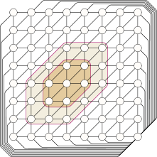
Figure 1: The graph $\Gamma_{8}$ with the first and second neighbourhood of an interior vertex marked.

See 1.4

Proof.

Fomin et al [18, Theorem 1] proved that for every apex-graph $H$ there exists a constant $c_{H}$ such that if $\operatorname{\mathbf{tw}}(G)\geqslant k$ and $G$ excludes $H$ as a minor, then $G$ has the graph $\Gamma_{c_{H}\cdot k}$ as a contraction minor. Here $\Gamma_{t}$ is the triangulated $t\times t$ grid where additionally one corner vertex is attached to all border vertices of the grid (Figure 1).

So assume that our input instance $(G,X,k)$ has treewidth $\operatorname{\mathbf{tw}}(G)\geqslant(5\sqrt{k}+10)/c_{H}$, then $G$ contains $\Gamma_{t}$ as a contraction minor with $t=5\sqrt{k}+10$. Let $X^{\prime}\subseteq V(\Gamma_{t})$ be the contracted forbidden vertices as defined above. As we observed earlier, every vertex in $X^{\prime}$ has at least one neighbour in $\Gamma_{t}$ which is not in $X^{\prime}$.

Claim.

$\Gamma_{t}$ contains a $1$-scattered set that avoids $X^{\prime}$ of size at least $k$.

Proof of claim.

Assume that the vertices of $\Gamma_{t}$ are labelled $v_{i,j}$, where $i,j\in[t]$ denote the row-index and column-index of the respective vertex in the grid.

Let $S^{\prime}:=\{v_{5x+3,5y+3}\mid 0\leqslant x\leqslant(t-5)/5~{}\text{and}~{}0\leqslant y\leqslant(t-5)/5\}$. The set $S^{\prime}$ is $2$-scattered in $\Gamma_{t}$ and has size at least $(t/5-2)^{2}$. Every vertex $u\in S^{\prime}$ is either not forbidden or it has a neighbour which is not forbidden, therefore we can construct a $1$-scattered set $S$ of the same size as follows: for every $u\in S^{\prime}$ we add a non-forbidden vertex from $N[u]$ to $S$. The claim follows now since $S$ has size at least

$$\big{(}\frac{t}{5}-2\big{)}^{2}=\big{(}\frac{5\sqrt{k}+10}{5}-2\big{)}^{2}=k.$$

∎

We conclude that if $G$ has treewidth at least $w:=(5\sqrt{k}+10)/c_{H}$, then $(G,X,k)$ is a YES-instance. Using the single-exponential $5$-approximation for treewidth [2], we can in time $2^{O(w)}n=2^{O(\sqrt{k})}n$ either find that $G$ has treewidth at least $w$ or we obtain a tree decomposition of width no larger than $5w$. In the latter case, we use the algorithm by Bazgan and Chopin to solve the problem in time $k^{O(w)}n=2^{O(\sqrt{k}\log k)}n$. Note that the total running time is bounded by $O(2^{o(k)}\cdot n)$, as claimed. ∎

5 Conclusion

We observed that the problem Harmless Set is in for sparse graph classes due to existing machinery. Therefore, we investigated its tractability in the kernelization sense and found that Harmless Set admits a polynomial sparse kernel. In the case of $p$-Bounded Harmless Set we even proved a linear sparse kernel. We expect these results to extend to nowhere dense classes.

On the negative side, we demonstrated that sparseness alone does not make the problem tractable. While the problem is in when parametrised by treewidth and solution size, we showed that it is in fact [1]-hard when only parametrised by treewidth. Our reduction shows even more, namely that most sparse parameters (treedepth, pathwidth, feedback vertex set) can be ruled out as the problem is already hard when parametrised by a modulator to a $2$-spider-forest.

We conjecture—and leave as an interesting open problem—that Harmless Set is already hard when parametrised by a modulator to a starforest.

Appendix 0.A Appendix

See 1

Proof.

By Observation 1, Harmless Set is equivalent to $(k+1)$-Bounded Harmless Set. Given an instance $(G,t,k)$ of the former, we can easily transform it into an instance $(G,t^{\prime},k)$ of the latter where $t^{\prime}(v)=\min\{t(v),k+1\}$.

We create the formula $\varphi^{HS}$ and prove that it defines Harmless Set.

Let $\psi(S,G,v)$ be the formula $\exists_{\leqslant t(v)}u.(v,u)\in E(G)\land u\in S$. Then $\varphi^{HS}_{k}(S,G)=((|S|=k)\land\forall v.\psi(S,G,v))$. expresses that $S$ is a harmless set of size $k$. Note that the expressions $|S|=k$ and $\exists_{\leqslant t(v)}$ are both expressible in FOL, though the size of the resulting formula depends on $k$ and $\max_{v\in V}t(v)\leqslant k+1$.

We now apply the powerful result by Grohe, Kreutzer, and Siebertz [20] that a first-order sentence $\phi$ can be decided in time $O(n^{1+\varepsilon})$ for any $\varepsilon>0$ in nowhere dense classes. This algorithm is (non-uniformly) , concluding the proof. ∎

See 3

Proof.

Given $G$, we use Theorem 2.2 to compute a $d$-dominating set $D^{\prime}$ of $A$ with $|D^{\prime}|=O(\operatorname{\mathbf{dom}}_{d}(G,A))$ in polynomial time. Afterwards, we compute the $(r+d)$-projection closure $D$ of $D^{\prime}$, by Lemma 2 we have that $|D^{\prime}|=O(|D|)$ and therefore $|D|=O(\operatorname{\mathbf{dom}}_{d}(G,A))$. Let $A^{\prime\prime}:=A\setminus D$, we will choose the polynomial $p_{r}$ so that $A^{\prime\prime}$ is still large enough for the following arguments to go through.

Define the equivalence relation $\sim_{D}$ over $A^{\prime\prime}$ via

$$a\sim_{D}a^{\prime}\iff\pi^{r+d}_{D}[a]=\pi^{r+d}_{D}[a^{\prime}].$$

By Lemma 1, the number of classes in $A^{\prime\prime}/\sim_{D}$ is bounded by $O(|D|)$; by an averaging argument we have at least one class $[a]\in A^{\prime\prime}/\sim_{D}$ of size

$$\big{|}[a]\big{|}=\Omega\Big{(}\frac{|A^{\prime\prime}|}{|D|}\Big{)}=\Omega\Big{(}\frac{|A|-|D|}{|D|}\Big{)}.$$

Let $R^{\prime\prime}=P^{r+d}_{D}(a)$, the $(r+d)$-projection of $[a]$’s members onto $D$. By our earlier application of Lemma 2 we have that $|R^{\prime\prime}|=|P^{r+d}_{D}(a)|=O(1)$.

We apply Theorem 2.1 with distance $r$ to the set $[a]$, let $g(r)$ be the function defined there. Using this notation, the algorithm of Theorem 2.1 provides us, in polynomial time, with a subset $A^{\prime}\subseteq[a]$ of size at least $|[a]|^{\frac{1}{g(r)}}$ and a constant-sized set $R^{\prime}\subseteq V(G)\setminus A^{\prime}$, such that $A^{\prime}$ is $r$-scattered in $G-R^{\prime}$.

Let $R:=R^{\prime}\cup R^{\prime\prime}$, by the above bounds on $R^{\prime}$ and $R^{\prime\prime}$ it follows that $|R|=O(1)$. By Lemma 1 the number of different $d$-projections onto $|R|$ is bounded by $O(|R|)$, so we can find a set $C\subseteq A^{\prime}$ with uniform $d$-projections onto $|R|$ of size at least

$$|C|\geqslant\frac{|A^{\prime}|}{|R|}=\Omega(|A^{\prime}|)=\Omega\Big{(}\big{(}\frac{|A|-|D|}{|D|}\big{)}^{\frac{1}{g(r)}}\Big{)}.$$

Since $|D|=O(\operatorname{\mathbf{dom}}_{d}(G,A))$, there exists a polynomial $p_{r}(t)=O((t^{1/g(r)}+1))$ such that $|A|\geqslant(t^{1/g(r)}+1)\cdot|D|$, which implies that

$$|C|=\Omega\Big{(}\big{(}\frac{|A|-|D|}{|D|}\big{)}^{\frac{1}{g(r)}}\Big{)}=\Omega(t).$$

Therefore we can choose $p_{r}(t)$ so that $|C|\geqslant t$, as claimed. ∎

References

- [1] Cristina Bazgan and Morgan Chopin. The complexity of finding harmless individuals in social networks. Discret. Optim., 14:170–182, 2014.
- [2] Hans L Bodlaender, Pål Grønås Drange, Markus S Dregi, Fedor V Fomin, Daniel Lokshtanov, and Michał Pilipczuk. A 5-approximation algorithm for treewidth. SIAM Journal on Computing, 45(2):317–378, 2016.
- [3] Ning Chen. On the approximability of influence in social networks. SIAM Journal on Discrete Mathematics, 23(3):1400–1415, 2009.
- [4] Wei Chen, Alex Collins, Rachel Cummings, Te Ke, Zhenming Liu, David Rincon, Xiaorui Sun, Yajun Wang, Wei Wei, and Yifei Yuan. Influence maximization in social networks when negative opinions may emerge and propagate. In Proceedings of the 2011 siam international conference on data mining, pages 379–390. SIAM, 2011.
- [5] Wei Chen, Laks VS Lakshmanan, and Carlos Castillo. Information and influence propagation in social networks. Synthesis Lectures on Data Management, 5(4):1–177, 2013.
- [6] Wei Chen, Yajun Wang, and Siyu Yang. Efficient influence maximization in social networks. In Proceedings of the 15th ACM SIGKDD international conference on Knowledge discovery and data mining, pages 199–208, 2009.
- [7] Marek Cygan, Fedor V Fomin, Łukasz Kowalik, Daniel Lokshtanov, Dániel Marx, Marcin Pilipczuk, Michał Pilipczuk, and Saket Saurabh. Parameterized algorithms. Springer, 2015.
- [8] Anuj Dawar. Finite model theory on tame classes of structures. In International Symposium on Mathematical Foundations of Computer Science, pages 2–12. Springer, 2007.
- [9] Anuj Dawar. Homomorphism preservation on quasi-wide classes. Journal of Computer and System Sciences, 76(5):324–332, 2010.
- [10] Erik D. Demaine and MohammadTaghi Hajiaghayi. The bidimensionality theory and its algorithmic applications. Comput. J., 51(3):292–302, 2008.
- [11] Reinhard Diestel. Graph Theory 5th edition. Graduate texts in mathematics, volume 173. Springer, 2016.
- [12] Pedro Domingos and Matt Richardson. Mining the network value of customers. In Proceedings of the seventh ACM SIGKDD international conference on Knowledge discovery and data mining, pages 57–66, 2001.
- [13] Pål Grønås Drange, Markus Sortland Dregi, Fedor V. Fomin, Stephan Kreutzer, Daniel Lokshtanov, Marcin Pilipczuk, Michał Pilipczuk, Felix Reidl, Fernando Sanchez Villaamil, Saket Saurabh, Sebastian Siebertz, and Somnath Sikdar. Kernelization and sparseness: the case of dominating set. In 33rd Symposium on Theoretical Aspects of Computer Science, STACS 2016, volume 47 of LIPIcs, pages 31:1–31:14. Schloss Dagstuhl - Leibniz-Zentrum für Informatik, 2016.
- [14] Paul A Dreyer Jr and Fred S Roberts. Irreversible -threshold processes: Graph-theoretical threshold models of the spread of disease and of opinion. Discrete Applied Mathematics, 157(7):1615–1627, 2009.
- [15] Zdeněk Dvořák. Constant-factor approximation of the domination number in sparse graphs. Eur. J. Comb., 34(5):833–840, 2013.
- [16] David Easley and Jon Kleinberg. Networks, crowds, and markets, volume 8. Cambridge university press, 2010.
- [17] Carl Einarson and Felix Reidl. A general kernelization technique for domination and independence problems in sparse classes. In 15th International Symposium on Parameterized and Exact Computation, IPEC 2020, December 14-18, 2020, Hong Kong, China (Virtual Conference), volume 180 of LIPIcs, pages 11:1–11:15. Schloss Dagstuhl - Leibniz-Zentrum für Informatik, 2020.
- [18] Fedor V Fomin, Petr Golovach, and Dimitrios M Thilikos. Contraction bidimensionality: the accurate picture. In European Symposium on Algorithms, pages 706–717. Springer, 2009.
- [19] Ajinkya Gaikwad and Soumen Maity. The harmless set problem. CoRR, abs/2111.06267, 2021.
- [20] Martin Grohe, Stephan Kreutzer, and Sebastian Siebertz. Deciding first-order properties of nowhere dense graphs. J. ACM, 64(3):17:1–17:32, 2017.
- [21] David Kempe, Jon Kleinberg, and Éva Tardos. Maximizing the spread of influence through a social network. In Proceedings of the ninth ACM SIGKDD international conference on Knowledge discovery and data mining, pages 137–146, 2003.
- [22] David Kempe, Jon Kleinberg, and Éva Tardos. Influential nodes in a diffusion model for social networks. In International Colloquium on Automata, Languages, and Programming, pages 1127–1138. Springer, 2005.
- [23] Stephan Kreutzer, Roman Rabinovich, and Sebastian Siebertz. Polynomial kernels and wideness properties of nowhere dense graph classes. ACM Trans. Algorithms, 15(2):24:1–24:19, 2019.
- [24] Hendrik W Lenstra Jr. Integer programming with a fixed number of variables. Mathematics of operations research, 8(4):538–548, 1983.
- [25] Jaroslav Nešetřil and Patrice Ossona De Mendez. First order properties on nowhere dense structures. The Journal of Symbolic Logic, 75(3):868–887, 2010.
- [26] Jaroslav Nešetřil and Patrice Ossona de Mendez. Grad and classes with bounded expansion I. Decompositions. Eur. J. Comb., 29(3):760–776, 2008.
- [27] Hung T Nguyen, My T Thai, and Thang N Dinh. Stop-and-stare: Optimal sampling algorithms for viral marketing in billion-scale networks. In Proceedings of the 2016 international conference on management of data, pages 695–710, 2016.
- [28] Nam P Nguyen, Guanhua Yan, My T Thai, and Stephan Eidenbenz. Containment of misinformation spread in online social networks. In Proceedings of the 4th Annual ACM Web Science Conference, pages 213–222, 2012.
- [29] Serge A. Plotkin, Satish Rao, and Warren D. Smith. Shallow excluded minors and improved graph decompositions. In Daniel Dominic Sleator, editor, Proceedings of the Fifth Annual ACM-SIAM Symposium on Discrete Algorithms. 23-25 January 1994, Arlington, Virginia, USA, pages 462–470. ACM/SIAM, 1994.
- [30] Felix Reidl, Fernando Sánchez Villaamil, and Konstantinos Stavropoulos. Characterising bounded expansion by neighbourhood complexity. European Journal of Combinatorics, 75:152–168, 2019.
- [31] Matthew Richardson and Pedro Domingos. Mining knowledge-sharing sites for viral marketing. In Proceedings of the eighth ACM SIGKDD international conference on Knowledge discovery and data mining, pages 61–70, 2002.
- [32] FS Roberts. Graph-theoretical problems arising from defending against bioterrorism and controlling the spread of fires. In Proceedings of the DIMACS/DIMATIA/Renyi combinatorial challenges conference, Piscataway, NJ, 2006.