Structural dynamics of polycrystalline graphene

Abstract

The exceptional properties of the two-dimensional material graphene make it attractive for multiple functional applications, whose large-area samples are typically polycrystalline. Here, we study the mechanical properties of graphene in computer simulations and connect these to the experimentally relevant mechanical properties. In particular, we study the fluctuations in the lateral dimensions of the periodic simulation cell. We show that over short time scales, both the area $A$ and the aspect ratio $B$ of the rectangular periodic box show diffusive behavior under zero external field during dynamical evolution, with diffusion coefficients $D_{A}$ and $D_{B}$ that are related to each other. At longer times, fluctuations in $A$ are bounded, while those in $B$ are not. This makes the direct determination of $D_{B}$ much more accurate, from which $D_{A}$ can then be derived indirectly. We then show that the dynamic behavior of polycrystalline graphene under external forces can also be derived from $D_{A}$ and $D_{B}$ via the Nernst-Einstein relation. Additionally, we study how the diffusion coefficients depend on structural properties of the polycrystalline graphene, in particular, the density of defects.

I Introduction

Graphite is a material in which layers of carbon atoms are stacked relatively loosely on top of each other. Each layer consists of carbon atoms, arranged in a honeycomb lattice. A single such layer is called graphene. This material has many exotic properties, both mechanical and electronic. Experimentally produced samples of graphene are usually polycrystalline, containing many intrinsic [1, 2, 3], as well as extrinsic [4] lattice defects. Unsaturated carbon bonds are energetically very costly [5, 6, 7, 8, 9], and therefore extremely rare in the bulk of the material. Polycrystalline graphene samples are therefore almost exclusively three-fold coordinated, and well described by a continuous random network (CRN) model [10], introduced by Zachariasen almost 90 years ago.

Polycrystalline graphene is continuously evolving in time, from one CRN-like state to another. A mechanism by which such a topological change can happen, was introduced by Wooten, Winer, and Weaire (WWW) in the context of the the simulation of samples of amorphous Si and Ge. This so-called WWW algorithm became the standard modeling approach for the dynamics of these kind of models [11, 12].

In the WWW approach, a configuration $C_{i}$ consists of a list of the coordinates of all $N$ atoms, coupled with an explicit list of the bonds between them. From this configuration $C_{i}$, a trial configuration $C^{\prime}_{i}$ is produced via a bond transposition: a sequence of carbon atoms $\{i,j,k,l\}$ is selected, connected with explicit bonds $i$-$j$, $j$-$k$ and $k$-$l$. The first and last of these bonds are then replaced by bonds $i$-$k$ and $j$-$l$, while bond $j$-$k$ is preserved. After this change in topology, the atoms are allowed to relax their positions. This simulation approach requires a potential that uses the explicit list of bonds, for instance the Keating potential [13] for amorphous silicon. The resulting configuration is then called the trial configuration $C^{\prime}_{i}$. The proposed change to this trial configuration is either accepted, i.e. $C_{i+1}=C^{\prime}_{i}$, or rejected, i.e. $C_{i+1}=C_{i}$. The acceptance probability is determined by the energy difference via the Metropolis criterion:

$$P=\min\{1,\exp(-\beta\Delta E)\},$$ (1)

where $\beta=(k_{B}T)^{-1}$, with Boltzmann constant $k_{B}$ and temperature $T$, and $\Delta E=E(C^{\prime})-E(C)$ is the change in energy due to the bond transposition. In this way, the simulation produces a Markov chain $C_{0}\dots C_{M}$, satisfying detailed balance.

The properties of polycrystalline graphene sheets have been a topic of intense research already for some time [14, 15, 16, 17, 18]. More recently, Ma et al. reported that the thermal conductivity of polycrystalline graphene films dramatically decreases with decreasing grain size [19]. The work of Gao et al. shows that the existence of single-vacancy point defect can reduce the thermal conductivities of graphene [20]. Wu et al. reported the magnetotransport properties of zigzag-edged graphene nanoribbons on an h-BN substrate [21]. Additionally, strain effects on the transport properties of triangular and hexagonal graphene flakes were studied in the work of Torres et al. [22].

This article reports on the dynamical properties of polycrystalline graphene. In particular, we study two geometric quantities that are readily accessible in computer simulations without having a clear experimental counterpart. In our simulations, the $L_{x}\times L_{y}$ graphene sample is rectangular, with periodic boundary conditions in the $x$- and $y$-directions; the quantities of interest are the area $A=L_{x}L_{y}$ and the aspect ratio $B=L_{x}/L_{y}$, and their mean square displacements (MSDs) under simulations in which the dynamics is the WWW algorithm. The results show that in the absence of external forces, MSD_A and MSD_B initially both increase linearly in time. At longer times, MSD_A saturates due to geometric limitations, while MSD_B keeps increasing linearly at all times. We measure the diffusion coefficients $D_{A}$ and $D_{B}$, and demonstrate that the two are related.

We then continue to show that $D_{A}$ and $D_{B}$ govern the response of the sample to stretching and shear forces respectively, following the Nernst-Einstein relation.

The main relevance of the research presented here lies in establishing the relation between observables that are readily accessible in simulations but without a clear experimental counterpart ($A$ and $B$ and their dynamics), and mechanical properties of real-life graphene (e.g. response to external stretching and shear forces). Additionally, we demonstrate a clear relation between MSD_A and MSD_B, thereby also relating the bulk- and the shear-properties. Thus far, much less is known about this shape fluctuation-driven diffusive behavior; our work provides insight into the dynamics and mechanics of polycrystalline graphene.

II The model

For simulating graphene, we use a recently developed effective semiempirical elastic potential [23]:

$$E_{0}=\frac{3}{16}\frac{\alpha}{d^{2}}\sum_{i,j}(r_{ij}^{2}-d^{2})^{2}+\frac{3}{8}\beta d^{2}\sum_{j,i,k}\left(\theta_{jik}-\frac{2\pi}{3}\right)^{2}$$ (2)

$$+\gamma\sum_{i,jkl}r_{i,jkl}^{2}.$$

Here, $r_{ij}$ is the distance between two bonded atoms, $\theta_{jik}$ is the angle between the two bonds connecting atom $i$ to atoms $j$ and $k$, and $r_{i,jkl}$ is the distance between atom $i$ and the plane through the three atoms $j$, $k$ and $l$ connected to atom $i$. The parameter $\alpha=26.060$ eV/Ų controls bond-stretching and is fitted to the bulk modulus, $\beta=5.511$ eV/Ų controls bond-shearing and is fitted to the shear modulus, $\gamma=0.517$ eV/Ų describes the stability of the graphene sheet against buckling, and $d=1.420$ Å is the ideal bond length for graphene. The parameters in the potential (2) are obtained by fitting to DFT calculations [23].

This potential has been used for the study of various mechanical properties of single-layer graphene, such as the vibrational density of states of defected and polycrystalline graphene [24] as well as of various types of carbon nanotubes [25], the structure of twisted and buckled bilayer graphene [26], the shape of nanobubbles trapped under a layer of graphene [25], and the discontinuous evolution of defected graphene under stretching [27].

The initial polycrystalline graphene samples are generated as in [28]. Here, $N/2$ random points are placed in a square simulation box with periodic boundary conditions, and the Voronoi diagram is generated: around each random point, its Voronoi cell is the region in which this random point is nearer than any other random point. We then translate the boundaries between neighboring Voronoi cells into bonds, and the locations where three boundaries meet into atomic positions. In this way, we have created a three-fold coordinated CRN which is homogeneous and isotropic (i.e. does not have preferred directions). It is, however, an energetically unfavorable configuration; therefore, we then evolve the sample using the improved bond-switching WWW algorithm to relax it, while preserving crystalline density.

Up to this point, the sample is completely planar (i.e., all $z$-coordinates are zero). After some initial relaxation, we then assign small random numbers to the $z$-coordinates followed by energy minimization, which results in a buckled configuration. At this point, we also allow the box lengths $L_{x}$ and $L_{y}$ to relax. We do not relax the box lengths already in poorly relaxed samples, because then the sheet tends to develop all kinds of unphysical structures.

In our implementation, we use the fast inertial relaxation engine algorithm (FIRE) for local energy minimization [29]; the values of the parameters in this algorithm (${N_{\min}}$, ${f_{inc}}$, ${f_{dec}}$, ${\alpha_{start}}$ and ${f_{\alpha}}$) are taken as suggested in Ref. [30]. Figure 1 presents an initial polycrystalline graphene sample with periodic boundary condition generated from a Voronoi diagram and evolved based on the WWW-algorithm.

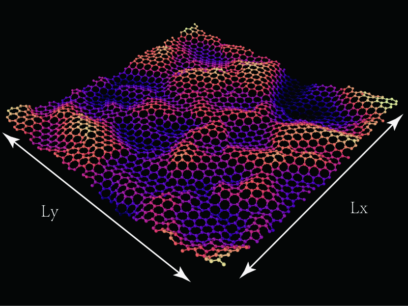
Figure 1: (color online) An initial buckled polycrystalline graphene sample with periodic boundary condition generated from a Voronoi diagram and evolved based on the WWW-algorithm. $L_{x}$ and $L_{y}$ represent the lateral dimensions of the sample.

III Dynamics of fluctuations in sample shapes

The oblong polycrystalline graphene sheet in our simulations has lengths $L_{x}$ and $L_{y}$ in the $x$- and the $y$-directions respectively, as shown in Fig. 1. These are not fixed quantities, but they fluctuate when bond transpositions are made.

Given that the sample is essentially two-dimensional, throughout this paper we consider two geometric quantities defined as follows:

$$A(t)=L_{x}(t)L_{y}(t)\quad\mbox{and}\quad B(t)=L_{x}(t)/L_{y}(t).$$ (3)

Physically, for a flat, rectangular and homogeneous isotropic sample, the stiffness matrix is reduced and the mechanical properties of system can be efficiently characterized by two independent in-plane modes due to orthorhombic symmetry, It is easiest to associate $A(t)$ and $B(t)$ to fluctuations in the sample shape in the “bulk” and the “shear” modes respectively at the macroscopic scale without these symmetries breaking. We then track the dynamics of shape fluctuations of the sample in terms of their mean-square displacements MSD${}_{A}(t)=\langle[A(t)-A(0)]^{2}\rangle$ and MSD${}_{B}(t)=\langle[B(t)-B(0)]^{2}\rangle$, with the angular brackets denoting ensemble averages for a sample of fixed number of atoms and (more or less) constant density of defects. (We will soon see that the diffusion coefficients are functions of both these quantities.) Characteristic fluctuations in $A$ and $B$ for a sample with 1352 atoms are shown in Fig. 2 panel (a), and correspondingly, their MSDs are shown in panels (b) and (c). Therein we find that fluctuations in $A$ are relatively much smaller in magnitude than those in $B$. Intuitively this makes sense, since relaxations through the shear mode is energetically much more favorable than through the bulk mode. This is also reflected in the MSDs. After a linear increase in time, MSD_A saturates at longer times, while MSD_B increases linearly at all times. From the data for MSD_A before it saturates, and MSD_B at all times, we identify the diffusion coefficients $D_{A}$ and $D_{B}$, obtained from fitting the data to the relation given by

$$\mbox{MSD}(t)=2Dt.$$ (4)

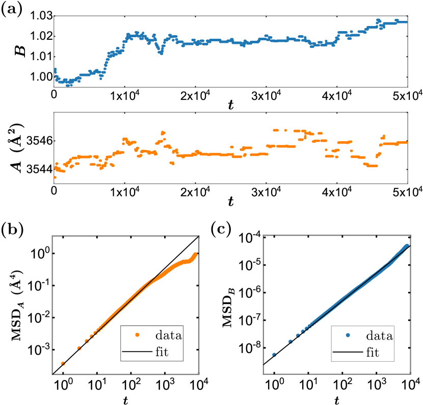
Figure 2: (color online) (a) Typical fluctuations in $A$ and $B$ in time for a sample with $N=1352$; note that the range of fluctuations in $B$ are considerably higher than in $A$. (b) MSD${}_{A}(t)$ and MSD${}_{B}(t)$ for this sample. The measured diffusion coefficients, as per Eq. (4) are $D_{A}\approx 1.737\times 10^{-4}$ Å⁴/[MC unit] and $D_{B}\approx 2.544\times 10^{-9}$ [MC unit]^-1. See text for details.

Since time is measured in MC units (bond transposition moves are being attempted once per unit of MC time), and length is measured in Å, the units of $D_{A}$ and $D_{B}$ are Å⁴/[MC unit] and [MC unit]^-1 respectively. Time all throughout the paper is measured in MC units.

III.1 $D_{B}$ increases linearly with defect density

An interesting question is what determines $D_{B}$ for a sample with a given number of atoms $N$. As we expect $D_{B}$ to be equal to zero for a perfect graphene sample, our first guess is that $D_{B}$ might depend on the density of defects. In our computer simulations of perfectly three-fold coordinated networks, defects are topological, in particular rings which are not six-fold. A convenient measure of the defect density $\rho$ is then obtained by the number of such rings per area. Note that rings are almost exclusively 5-, 6- and 7-fold in the well-relaxed samples as we studied. Since 5- and 7-fold rings generally appear and disappear in pairs, one can expect that the ratio of N5/N7 (N represents the number of 5- for 7-fold rings) is close to unity.

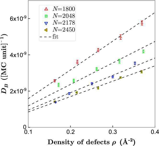
Figure 3: (color online) $D_{B}$ plotted for four differently-sized samples, each with four different defect densities (points: simulation data, lines: best fit passing through origin). Error bars represent standard error of the mean, obtained from the ensemble of simulation runs. See text for details.

In order to test our intuition, we simulate graphene samples for four different atom numbers (around $N=2000$), each with four different defect densities. The results are shown in Fig. 3. Points represent simulation data with statistical error bars, and dashes lines are best fit lines with each line passing through the origin (corresponding to $D_{B}=0$ at $\rho=0$). Even though there is no a priori reason for $D_{B}$ to increase linearly with $\rho$ for every value of $N$, Fig. 3 demonstrates that the linear scaling holds for the range of defect densities we simulated. Also clear is the decreasing trend in $D_{B}$ with increasing $N$ for a certain defect density. On a technical side, each point is obtained from averaging over 10 independent samples, and each sample is simulated 16 times over 30,000 attempted bond transpositions at a temperature of $kT=0.25$ eV within each run. We perform further averaging over the initial time. The CPU time of a single attempted bond transposition is on average 0.76 s for samples ($N$=2000).

III.2 Relation between $D_{A}$ and $D_{B}$

Further, since both $A$ and $B$ bear relations to $L_{x}$ and $L_{y}$, one would expect them to be related through these length parameters, which we establish below. In order to do so, having denoted the change in $A$ and $B$ over a small time interval $dt$ for samples with dimensions $L_{x}$ and $L_{y}$ by $dA$ and $dB$ respectively, we express them in terms of small changes $dL_{x}$ and $dL_{y}$ as

$$\langle dA^{2}\rangle = \left\langle\left[L_{y}dL_{x}+L_{x}dL_{y}\right]^{2}\right\rangle\quad\mbox{and}$$

$$\langle dB^{2}\rangle = \left\langle\frac{1}{L_{y}^{4}}\left[L_{y}dL_{x}-L_{x}dL_{y}\right]^{2}\right\rangle.$$ (5)

Using $\langle dL_{x}dL_{y}\rangle=0$ after an ensemble averaging, Eq. (5) leads to the simplified form

$$\langle dA^{2}\rangle = L_{y}^{2}\,\langle dL_{x}^{2}\rangle+L_{x}^{2}\,\langle dL_{y}^{2}\rangle\quad\mbox{and}$$

$$\langle dB^{2}\rangle = \frac{1}{L_{y}^{4}}\left[L_{y}^{2}\,\langle dL_{x}^{2}\rangle+L_{x}^{2}\,\langle dL_{y}^{2}\rangle\right],$$ (6)

i.e., $\langle dA^{2}\rangle/\langle dB^{2}\rangle=L_{y}^{4}$. If we extend this analysis to finite times, for which $L_{y}$ does not appreciably change, then we expect the ratio $D_{A}/D_{B}$ to behave $\sim L^{4}_{y}$.

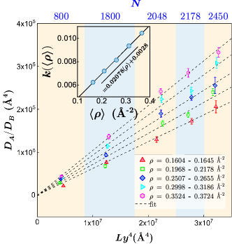
Figure 4: (color online) The ratio $D_{A}/D_{B}$ vs $L_{y}^{4}$ for different $N$-values and defects densities [points: simulation data, lines: best-fit of the form $D_{A}/D_{B}=k(\langle\rho\rangle)\,L^{4}_{y}$]. Error bars represent standard error of the mean, obtained from the ensemble of simulation runs. The points located a color bar are measured with the same $N$. The inner plot shows that $k(\langle\rho\rangle)$ also bears a linear relation with $\langle\rho\rangle$ obtained from averaging in the ranges: $k(\langle\rho\rangle)=0.02078\langle\rho\rangle+0.0028$.

In Fig. 4 we plot $D_{A}/D_{B}$ for $N$=800, 1800, 2048, 2178, 2450 and five different ranges with approximate defect densities. We indeed observe that $D_{A}/D_{B}\sim L_{y}^{4}$: once again, simulation data are shown as points, while the dashed lines are the best-fit $D_{A}/D_{B}=k(\rho)\,L^{4}_{y}$ lines through the data points. The $k$-values, summarized in Tab. 1, are plotted as an inset to Fig. 4. Here we determine $k$ by using statistical quantity $\langle\rho\rangle$ obtained from averaging in the ranges, these $k(\langle\rho\rangle)$ vs $\langle\rho\rangle$ points also lie on a straight line, whose best-fit estimate is $k(\langle\rho\rangle)=0.02078\langle\rho\rangle+0.0028$.

$\quad\langle\rho\rangle\quad$	$k(\langle\rho\rangle)$
0.16433	$\quad 6.24\times 10^{-3}\quad$
0.21065	$7.20\times 10^{-3}$
0.26154	$8.14\times 10^{-3}$
0.31323	$9.35\times 10^{-3}$
0.36670	$1.04\times 10^{-2}$

Table 1: Values of $k$ for different values of $\langle\rho\rangle$, corresponding to the best-fit $D_{A}/D_{B}=k(\langle\rho\rangle)\,L^{4}_{y}$ lines in Fig. 4.

$N$	$\langle L_{x,\text{initial}}\rangle$(Å)	$\langle L_{y,\text{initial}}\rangle$(Å)
800	45.35	45.72
1800	68.47	68.95
2048	73.91	72.58
2178	75.78	75.39
2450	80.15	80.38

Table 2: Dimensions of initial configurations obtained after optimization. Averaging for each $N$ was done over 5 ($\langle\rho\rangle$ values listed in the table 1) $\times$ 10 (independent samples) $\times$ 16 (repetitions).

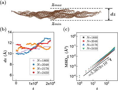
Figure 5: (color online) (a) A suspended graphene sample naturally tends to buckle, $dz$ is the thickness of the sample. (b) The variation of $dz$ for four differently-sized samples, the initial defects densities for all sample are fixed at around 0.15. (c) MSD_dz for these samples.

III.3 MSD in the $z$-direction

The graphene in our simulations is free-floating, and the presence of defects causes it to buckle, i.e., the carbon atoms show displacements in the out-of-plane direction. During bond transpositions, the buckling structure changes. To quantify the dynamics of buckling, we determine the minimal and maximal values of the $z$-coordinates of the atoms, and the difference $dz=z_{max}-z_{min}$; this is illustrated in the top panel of Fig. 5.

$$\text{MSD}_{dz}(t)=\langle[dz(t)-dz(0)]^{2}\rangle.$$ (7)

Analogous to our analysis of the dynamics of $L_{x}(t)$ and $L_{y}(t)$, we then determine the MSD_dz of $dz(t)$. The results for various system sizes are shown in figure 5, in samples with a defect density around 0.15, simulated at a temperature of $kT$ = 0.25 eV. Figure 5(b) shows that the $dz$ fluctuates around a level $\approx 11$ Å, which is the typical equilibrium amplitude of the buckling for these samples; out-of-plane displacement-related studies can be found in our previous simulations [24]. Figure 5(c) shows that the initial behavior is diffusive, with a diffusion coefficient that is insensitive to $N$.

III.4 Summary: defect density determines shape fluctuation dynamics

In summary so far, we have established that the density of defects determines $D_{B}$, and that the ratio $D_{A}/D_{B}=k(\langle\rho\rangle)L^{4}_{y}$ in Sec. III.2. Putting these results together then implies that the density of defects is the sole determining factor for the dynamics of fluctuations in the sample shapes.

IV Sample response to external forces

That the fluctuations in quantity $B$ lead to diffusive behavior without being limited by geometric constraints made us follow-up with the response of the samples to externally applied forces. In particular, if we apply a (weak) force $F_{B}$ to excite the shear mode, then we expect the (linear) response in terms of “mobility” $\mu_{B}$ in the relation $v_{B}=\mu_{B}F_{B}$ for the “deformation velocity $v_{B}$ of the sample along the $B$-direction” to satisfy the Einstein relation

$$\mu_{B}=\frac{D_{B}}{k_{B}T};\quad\mbox{i.e.,}\quad v_{B}=\frac{D_{B}}{k_{B}T}F_{B},$$ (8)

where $k_{B}$ is the Boltzmann constant and $T$ is the temperature of the sample.

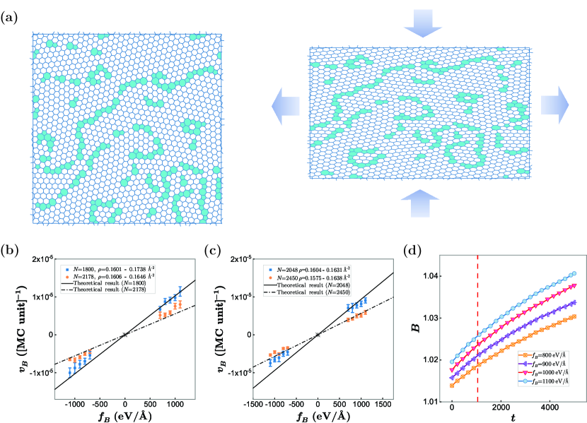
Figure 6: (color online) (a) A relaxed polycrystalline graphene sample. Elongated domains arise if the sample is stretched significantly within a short period of time. (b-c) $v_{B}$ directly measured vs. predicted by the Nernst-Einstein relation (8). Error bars represent standard error of the mean, obtained from the ensemble of simulation runs. (d) Change in $B$ in time when a constant stretching force is applied to the sample, restoring tendencies of elongated domains cause slower-than-linear increases at longer times ($t>1000$).

In order to check for this relation in our simulations, we add an extra “force term” in the Hamiltonian in Eq. (2), to have the new Hamiltonian as

$$E=E_{0}+c\frac{L_{x}}{L_{y}}\equiv E_{0}+cB,$$ (9)

and calculate $v_{B}$ in the following manner, for the applied force $F_{B}=\partial E/\partial B=c$.

The behavior of the aspect ratio $B$ as a function of time, under a constant force $f_{B}$, is shown in figure 6a, for forces $f_{B}=\pm 800,900,1000$ and 1100 eV/Å. The curves in this figure are obtained by averaging over 8 independent samples, each one simulated 32 times for each value of the force. At relatively short times, $B$ increases linearly in time. Afterwards, the shear rate has a tendency to slow down. We speculate that this slowing down at longer times might be due to deformation of domains: Initially, these crystalline domains are isotropic, but after the sample has sheared over quite some distance, the domains become elongated. The tendency to restore isotropy makes the sample resist further deformation. This is illustrated in fig. 6a. There is no a priori reason to assume that the increase in energy due to shearing is harmonic. In analogy to the quartic increase of the length of a circle under this type of deformation, we rather expect highly non-linear behavior. At short times, where the sample has not deformed significantly, the change in $B$ as a response to the force $f_{B}$ is expected to be given by the Nernst-Einstein equation Eq. (7). To test this, we obtained the short-time shear velocity $v_{B}$ by fitting the slopes in figure 6a for the various forces. These measurements of $v_{B}$ are plotted in figures 6b and 6c, as a function of $f_{B}$. Also plotted in figures 6b and 6c are the theoretical expectations as obtained from the Nernst-Einstein equation, in which we used the earlier obtained values for $D_{B}$. The figures 6b and 6c show agreement between the direct measurements of $v_{B}$ and the theoretical expectations, indicating that with forces of these strengths the mechanical response is well-understood.

V Conclusion

Computer simulations of materials at the atomistic level usually involve samples containing typically a few thousand atoms, with periodic boundary conditions. Quantities that can be easily and reliably measured in such simulations, are for instance the evolution in time of the lateral sizes of the periodic box, such as their fluctuations. In the simulations on graphene as presented here, the directly observable quantities are the lateral lengths $L_{x}$ and $L_{y}$ of the rectangular periodic box. The dynamics of $L_{x}$ and $L_{y}$ are coupled and can be better understood by considering the area $A=L_{x}L_{y}$ and aspect ratio $B=L_{x}/L_{y}$. Specifically, we concentrate on the mean-squared displacements of $A$ and $B$. At short times, in which only a few atomic rearrangements occur, $A$ and $B$ show ordinary diffusive behavior, with diffusion coefficients $D_{A}$ and $D_{B}$. We show that if the changes in $L_{x}$ and $L_{y}$ are uncorrelated, $D_{A}$ and $D_{B}$ can be obtained from each other. While this might not seem very surprising at first sight, it does connect the dynamics of shear mode and bulk mode — two quantities that are usually assumed to be uncorrelated — at short times.

At longer times, $A$ and $B$ show different behavior. Graphene has a characteristic density, which translates directly into a preferred value for $A$ around which it fluctuates. The amplitude of the fluctuations in $A$ are determined by the bulk modulus, which is an equilibrium property and therefore computationally obtainable from simulations without realistic dynamics. The aspect ratio $B$ does not have an energetically preferred value, and its diffusive behavior is therefore unrestricted. A practical consequence is that in simulations the quantity $D_{B}$ can be determined more accurately than $D_{A}$, as the latter shows a crossover from short-time diffusive behavior to late-time saturation.

In our simulations, we have studied samples of polycrystalline graphene with a variation in the amount of structural relaxation, the size of the crystalline domains, and the density of structural defects (mainly fivefold and sevenfold rings). In our simulations, we show a linear relation between the number of such structural defects and the diffusion coefficient $D_{B}$. In well-relaxed samples, large crystalline domains are separated from each other by rows of structural defects. Consequently, the number of defects decreases linearly with the average domain size. We therefore expect also that the diffusion coefficient $D_{B}$ decreases linearly with the average domain size. In this context it will be useful to deepen this connection to domain size engineering [31, 32, 33], fabrication of polycrystalline graphene [34, 35, 36], mechanics of grain boundaries [37, 38].

From a materials science point of view, as well as from an experimental point of view, the mechanical behavior of a sample of graphene under external forces is important. We show that the deformation of graphene under an external shear force is related to the quantity $D_{B}$ which is readily accessible in simulations, via the Nerst-Einstein relation. For this purpose, the external shear force is translated into a force $f_{B}$ on the quantity $B$, after which the shear rate $v_{B}=\partial B/\partial t$ can be obtained from equation (8), in which the diffusion coefficient $D_{B}$ is used. And the mechanical deformation can then be readily obtained from $v_{B}$.

We have limited ourselves to a relatively modest dynamical range of $L_{x}$ and $L_{y}$, as well as relatively mild deformation forces. Consequentially, in our simulations the domains do not get deformed to elongated shapes but retain circular symmetry. If the material would be stretched significantly in a time that is short enough to rule out complete structural rearrangement, elongated domains should arise, and the sample would experience restoring forces back towards its original shape. This is illustrated in Fig. 6(a). We speculate that this mechanism would actually slow down the shearing process, making the shear distance non-linear in time. Our simulations show signs of the onset of decreasing shear rate in time [Fig. 6(d)]. A quantitative study of this phenomenon, in which the possible relation between elongation of domains and non-linear shear is investigated both in experiments and mechanism, such as strengthening or weakening of graphene [39, 40, 41], fracture toughness [42, 43, 44], mechanical mutability [45], requires very long simulations, which we will pick up in future work. We believe these investigations enhance our understanding of the mechanical properties of polycrystalline graphene.