TUM-HEP-1332/21

November 23, 2021

QCD factorization for the four-body leptonic
$B$-meson decays

Chao Wang${}^{a,\,b}$ , Yu-Ming Wang^a , Yan-Bing Wei${}^{a,\,c}$
^a School of Physics, Nankai University,
Weijin Road 94, 300071 Tianjin, China
^b Department of Mathematics and Physics,
Meicheng East Road 1, Huaiyin Institute of Technology,
223200 Huaian, Jiangsu, China
^c Physik Department T31,
James-Franck-Straße 1, Technische Universität München,
D–85748 Garching, Germany

Employing the QCD factorization formalism we compute $B_{u}^{-}\to\gamma^{\ast}\,\ell\,\bar{\nu}_{\ell}$ form factors with an off-shell photon state possessing the virtuality of order $m_{b}\,\Lambda_{\rm QCD}$ and $m_{b}^{2}$, respectively, at next-to-leading order in QCD. Perturbative resummation for the enhanced logarithms of $m_{b}/\Lambda_{\rm QCD}$ in the resulting factorization formulae is subsequently accomplished at next-to-leading logarithmic accuracy with the renormalization-group technique in momentum space. In particular, we derive the soft-collinear factorization formulae for a variety of the subleading power corrections to the exclusive radiative $B_{u}^{-}\to\gamma^{\ast}\,W^{\ast}$ form factors with a hard-collinear photon at ${\cal O}(\alpha_{s}^{0})$. We further construct the complete set of the angular observables governing the full differential distribution of the four-body leptonic decays $B_{u}^{-}\to\ell^{\prime}\,\bar{\ell}^{\prime}\,\ell\,\bar{\nu}_{\ell}$ with $\ell,\,\ell^{\prime}\in\{e,\,\mu\}$ and then perform an exploratory phenomenological analysis for a number of decay observables accessible at the LHCb and Belle II experiments, with an emphasis on the systematic uncertainties arising from the shape parameters of the leading-twist $B$-meson light-cone distribution amplitude in heavy quark effective theory.

1 Introduction

The exclusive leptonic decays of the charged $B_{u}^{-}$-meson are of paramount importance for exploring the complex quark-flavour dynamics in the Standard Model (SM) and for probing the nonstandard flavour-changing mechanisms beyond the electroweak scale. However, the helicity suppression of the two-body leptonic $B_{u}^{-}\to\mu\,\bar{\nu}_{\mu}$ decay process is expected to yield the tiny branching fraction of ${\cal O}(10^{-7})$, which prevents the decisive measurements at the BaBar and Belle experiments with more than $5\,\sigma$ significance (see [1, 2, 3, 4] for the available searches at the $e^{+}e^{-}$ colliders). On the other hand, the radiative leptonic $B_{u}^{-}\to\gamma\ell\bar{\nu}_{\ell}$ decays with an energetic photon will evidently lift such unwanted helicity suppression [5, 6, 7, 8], at the price of introducing the additional suppression from the electromagnetic coupling constant and from the Lorenz invariant three-body phase space factor. Reconstructing the $B$-meson decay vertex with just a single charged particle will unfortunately bring about the tremendous challenges for searching $B_{u}^{-}\to\mu\,\bar{\nu}_{\mu}$ and $B_{u}^{-}\to\gamma\ell\bar{\nu}_{\ell}$ at the LHCb experiment. It is therefore advantageous to investigate the four-body leptonic decays $B_{u}^{-}\to\ell^{\prime}\,\bar{\ell}^{\prime}\,\ell\,\bar{\nu}_{\ell}$ with $\ell,\,\ell^{\prime}\in\{e,\,\mu\}$ with three charged tracks for the sake of facilitating the experimental reconstruction of the bottom-meson candidates in the hadronic collision environment and circumventing the helicity suppression mechanism applied to the two-body leptonic decays simultaneously. From the QCD perspective, the rare leptonic decays $B_{u}^{-}\to\ell^{\prime}\,\bar{\ell}^{\prime}\,\ell\,\bar{\nu}_{\ell}$ with the invariant mass of the lepton pair $(\ell^{\prime}\,\bar{\ell}^{\prime})$ of order $m_{b}\,\Lambda_{\rm QCD}$ will further provide us with the valuable information on the inverse moment of the twist-two $B$-meson distribution amplitude in heavy quark effective theory (HQET), which serves as an indispensable ingredient for the theory description of a variety of the exclusive $B$-meson decay observables [9, 10, 11, 12, 13, 14, 15, 16] based upon the heavy quark expansion as well as the dispersion technique. Moreover, the exclusive four-body decays $B_{u}^{-}\to\gamma^{\ast}(\to\ell^{\prime}\,\bar{\ell}^{\prime})\,\ell\,\bar{\nu}_{\ell}$ with the four-momentum ($p_{\mu}$) of the intermediate photon state satisfying $p^{2}\sim{\cal O}(m_{b}^{2})$ are apparently of interest for addressing the “notorious” open issue of the systematic uncertainty due to the analytical continuation of the (local) operator product expansion (OPE) from the Euclidean to the Minkowskian domain in the practical applications [17, 18, 19].

In analogy to the exclusive electromagnetic penguin decays $B\to K^{(\ast)}\ell\bar{\ell}$ [20, 21], the presence of the vector-meson resonances (e.g., $\rho$, $\omega$, etc) in the $(\ell^{\prime}\,\bar{\ell}^{\prime})$ invariant mass spectrum of $B_{u}^{-}\to\ell^{\prime}\,\bar{\ell}^{\prime}\,\ell\,\bar{\nu}_{\ell}$ will invalidate the applicability of the perturbative factorization approach for evaluating the resulting hadronic tensor in the collinear regime of $p^{2}\sim{\cal O}(\Lambda_{\rm QCD}^{2})$. As a consequence, we will focus on the kinematical region of the virtuality of the photon state appearing in $B\to\gamma^{\ast}\,\ell\,\bar{\nu}_{\ell}$ above the light vector-meson threshold, in contrast to the previous phenomenological explorations in the entire kinematically allowed regions [22, 23] by employing the vector-meson-dominance (VMD) ansatz, which permits us to apply the appropriate OPE techniques for disentangling the strong interaction dynamics at the separated distance scales. In particular, QCD calculations of the four-body leptonic $B_{u}^{-}$-meson decays at leading power in an expansion in terms of $\Lambda_{\rm QCD}/m_{b}$ with the hard-collinear dilepton system resemble constructing the soft-collinear factorization formula for the vacuum-to-bottom-meson correlation function $T_{7B}^{\mu\nu}$ entering in the radiative leptonic $B_{d,s}\to\gamma\ell\bar{\ell}$ amplitude [11] generated by the $B$-type insertion of the effective weak operators . In addition, the nonperturbative hadronic dynamics imbedded in the timelike $B_{u}^{-}\to\gamma^{\ast}\ell\bar{\nu}_{\ell}$ form factors with an off-shell photon carrying the hard momentum $p_{\mu}\sim{\cal O}(m_{b})$ will be characterized by the bottom-meson decay constant $f_{B_{u}}$, which has been determined from the lattice-QCD simulation at $N_{f}=2+1+1$ with the relative precision of approximately $0.68\,\%$ [24]. As the power counting scheme for the virtuality of the photon state dictates factorization properties of the non-hadronic radiative $B_{u}^{-}\to\gamma^{\ast}\ell\bar{\nu}_{\ell}$ decay form factors, the non-local hadronic matrix element defined by the time-ordered product of the weak transition current $\bar{u}\,\gamma_{\mu}\,(1-\gamma_{5})\,b$ and the bottom-quark electromagnetic current will result in an unsuppressed contribution at $p^{2}\sim{\cal O}(m_{b}^{2})$ in the heavy quark expansion.

In contrast to the radiative leptonic $B_{u}^{-}\to\gamma\ell\bar{\nu}_{\ell}$ decays with an on-shell photon state, it necessitates the introduction of three independent hadronic form factors to parameterize the non-local matrix element encoding the QCD effects for the four-body leptonic decays $B_{u}^{-}\to\gamma^{\ast}(\to\ell^{\prime}\,\bar{\ell}^{\prime})\,\ell\,\bar{\nu}_{\ell}$ by implementing the two nontrivial constraints from the Ward-Takahashi identity . Consequently, one of the major technical objectives of the present paper consists in computing the leading-power contributions to the generalized form factors of $B_{u}^{-}(p_{B})\to\gamma^{\ast}(p)\,\ell(q_{1})\,\bar{\nu}_{\ell}(q_{2})$ in the heavy quark expansion based upon the soft-collinear effective theory (SCET) approach and the local OPE technique at $p^{2}\sim{\cal O}(m_{b}\,\Lambda_{\rm QCD})$ and $p^{2}\sim{\cal O}(m_{b}^{2})$ respectively, including the next-to-leading logarithmic (NLL) resummation for the parametrically large logarithms of $m_{b}/\Lambda_{\rm QCD}$ in the obtained factorization expression with the renormalization-group (RG) formalism. The yielding formulae for the radiative $B_{u}^{-}\to\gamma^{\ast}$ transition form factors with an off-shell hard-collinear photon can be further evaluated by postulating the complete momentum dependence of the leading-twist $B$-meson distribution amplitude rather than by introducing the inverse moment $\lambda_{B}$ and the first two inverse-logarithmic moments $\sigma_{B}^{(n)}$ at the NLL accuracy as in the case of computing the on-shell $B_{u}^{-}\to\gamma$ form factors [5, 6, 7, 8]. Furthermore, we will endeavour to carry out the factorization analysis for various subleading-power corrections to the exclusive rare $B_{u}^{-}\to\gamma^{\ast}\,W^{\ast}$ decay form factors in the hard-collinear $p^{2}$-regime with the aid of the two-particle and three-particle higher-twist HQET distribution amplitudes. In addition, the primary phenomenological new ingredient of our analysis consists in the comprehensive investigation of the full angular decay distribution for $B_{u}^{-}\to\gamma^{\ast}(\to\ell^{\prime}\,\bar{\ell}^{\prime})\,W^{\ast}(\to\ell\,\bar{\nu}_{\ell})$ in terms of five independent kinematical variables for both $\ell=\ell^{\prime}$ and $\ell\neq\ell^{\prime}$: the invariant masses of the dilepton system ($p^{2}$) and of the lepton-neutrino pair ($q^{2}$), the three angles $\theta_{1}$, $\theta_{2}$ and $\phi$ defined in Appendix A, which allows for the systematic construction of a numbers of observables accessible at the LHCb and Belle II experiments.

The outline of this presentation is as follows. We will set up the computational framework in Section 2 by establishing the general parametrization of the four-body leptonic $B$-meson decay amplitude to the lowest non-vanishing order in the electromagnetic interaction and by exploiting the interesting implications of the ${\rm U_{em}(1)}$ gauge symmetry on the emerged $B_{u}^{-}\to\gamma^{\ast}\,W^{\ast}$ decay form factors. The matching procedure ${\rm QCD\rightarrow SCET_{I}\rightarrow SCET_{II}}$ for the appearing $B$-meson-to-vacuum correlation function defined by the flavour-changing $b\to u$ weak current and the electromagnetic quark current carrying a hard-collinear momentum $p$ will be performed at leading power in $\Lambda_{\rm QCD}/m_{b}$ in Section 3 with the accustomed perturbative factorization technique, where the subleading power contribution from the virtual photon radiation off the heavy bottom-quark field will be also derived at leading order (LO) in the strong coupling constant with the OPE technique. In particular, the Ward-Takahashi relations of the generalized radiative $B$-meson decay form factors will be demonstrated explicitly at one loop. The non-local power suppressed corrections from a number of distinct sources (parametrized by the higher-twist bottom-meson distribution amplitudes) will be further addressed here by employing the HQET equations of motion at tree level. In Section 4 we will proceed to carry out the ${\rm QCD\rightarrow HQET}$ matching programme for the aforementioned $B$-meson-to-vacuum correlation function at ${\cal O}(\alpha_{s})$, where the factorization-scale independence of the achieved expressions for all the $B_{u}^{-}\to\gamma^{\ast}\,W^{\ast}$ form factors will be further verified at next-to-leading order (NLO) in QCD taking advantage of the RG evolution equation for the effective decay constant $\tilde{f}_{B}(\mu)$. Having at our disposal the factorized expressions for these hadronic transition form factors, we will turn to investigate their numerical implications with the three-parameter ansatz of the HQET $B$-meson distribution amplitude as proposed in [8] in Section 5, where the phenomenological aspects of the four-body leptonic $B$-meson decays will be subsequently explored with circumstances on the basis of the corresponding full differential distribution described by the five independent kinematical variables as previously mentioned. The concluding remarks and theory perspectives on the future improvements will be presented in Section 6. We collect in Appendix A the kinematics of the exclusive reaction $B_{u}^{-}\to\ell^{\prime}\,\bar{\ell}^{\prime}\,\ell\,\bar{\nu}_{\ell}$ with $\ell=\ell^{\prime}$ and $\ell\neq\ell^{\prime}$ and then present in Appendix B the explicit expressions of the angular coefficient functions entering the interference term of the full differential distribution for the four-body leptonic decay with identical lepton flavours.

2 Preliminaries

By analogy with the detailed discussions on the $B$-meson radiative leptonic decays [5, 6, 7, 8], the four-body leptonic $B_{u}^{-}\to\ell^{\prime}\,\bar{\ell}^{\prime}\,\ell\,\bar{\nu}_{\ell}$ decay amplitude can be expressed as

$${\cal A}(B_{u}^{-}\to\ell^{\prime}\,\bar{\ell}^{\prime}\,\ell\,\bar{\nu}_{\ell})$$

$$={G_{F}\,V_{ub}\over\sqrt{2}}\,\langle\ell^{\prime}(p_{1})\,\bar{\ell}^{\prime}(p_{2})\,\ell(q_{1})\,\bar{\nu}_{\ell}(q_{2})|\left[\bar{\ell}\gamma^{\mu}(1-\gamma_{5})\nu_{\ell}\right]\,\left[\bar{u}\gamma_{\mu}(1-\gamma_{5})b\right]|B_{u}^{-}(p_{B})\rangle\,,$$ (1)

where $p_{B}=m_{B}\,v=p+q$ is the four-momentum of the $B$-meson momentum with $v$ being its velocity, $p=p_{1}+p_{2}$ and $q=q_{1}+q_{2}$ denote the outgoing momenta carried by the off-shell photon and the $W^{\ast}$ boson in the cascade decay process $B_{u}^{-}\to\gamma^{\ast}(\to\ell^{\prime}\,\bar{\ell}^{\prime})\,W^{\ast}(\to\ell\,\bar{\nu}_{\ell})$, respectively. It further proves convenient to work in the rest frame of the $B$-meson and to introduce the two light-cone vectors $n_{\alpha}$ and $\bar{n}_{\alpha}$ fulfilling the general relations $n^{2}=\bar{n}^{2}=0$ and $n\cdot\bar{n}=2$ such that

$$p_{\alpha}={n\cdot p\over 2}\,\bar{n}_{\alpha}+{\bar{n}\cdot p\over 2}\,n_{\alpha}\,,\qquad q_{\alpha}={n\cdot q\over 2}\,\bar{n}_{\alpha}+{\bar{n}\cdot q\over 2}\,n_{\alpha}\,,\qquad v_{\alpha}={n_{\alpha}+\bar{n}_{\alpha}\over 2}\,.$$ (2)

Keeping the first-order contribution to the decay amplitude ${\cal A}(B_{u}^{-}\to\ell^{\prime}\,\bar{\ell}^{\prime}\,\ell\,\bar{\nu}_{\ell})$ in the electromagnetic interaction gives rise to following expression

$${\cal A}(B_{u}^{-}\to\ell^{\prime}\,\bar{\ell}^{\prime}\,\ell\,\bar{\nu}_{\ell}) = {G_{F}\,V_{ub}\over\sqrt{2}}\,{ig_{\rm em}^{2}\,Q_{\ell^{\prime}}\over p^{2}+i0}\,\left[\bar{\ell}^{\prime}(p_{1})\,\gamma^{\nu}\,\ell^{\prime}(p_{2})\right]\,$$ (3)

$$\times\,\{T_{\nu\mu}(p_{B},p)\,\left[\bar{\ell}(q_{1})\gamma^{\mu}(1-\gamma_{5})\nu_{\ell}(q_{2})\right]-\,i\,f_{B}\,p_{B}^{\mu}\,\,L_{\nu\mu}(p_{B},p)\}\,,$$

where the hadronic matrix element $T_{\nu\mu}$ and the leptonic rank-two tensor $L_{\nu\mu}$ are defined by

$$T_{\nu\mu}(p_{B},p) = \int d^{4}x\,e^{ip\cdot x}\,\langle 0|{\rm T}\{j_{\nu}^{\rm em}(x),\bar{u}(0)\gamma_{\mu}(1-\gamma_{5})b(0)\}|B_{u}^{-}(p_{B})\rangle\,,$$ (4)

$$L_{\nu\mu}(p_{B},p) = \int d^{4}x\,e^{ip\cdot x}\,\langle\ell(q_{1})\,\bar{\nu}_{\ell}(q_{2})|{\rm T}\{j_{\nu}^{\rm em}(x),\bar{\ell}(0)\gamma_{\mu}(1-\gamma_{5})\nu_{\ell}(0)\}|0\rangle\,.$$ (5)

The explicit form of the fermion electromagnetic current is given by

$$j_{\nu}^{\rm em}(x)=\sum_{q}Q_{q}\,\bar{q}(x)\gamma_{\nu}q(x)+\sum_{\ell}\,Q_{\ell}\,\bar{\ell}(x)\gamma_{\nu}\ell(x)\,,$$ (6)

and the $B$-meson decay constant in QCD is defined by the local axial-vector matrix element

$$\langle 0|\bar{u}\,\gamma^{\mu}\,\gamma_{5}\,b|B_{u}^{-}(p_{B})\rangle=i\,f_{B}\,p_{B}^{\mu}\,.$$ (7)

Taking advantage of the general decomposition of the hadronic tensor [6]

$$T_{\nu\mu}(p,q) = i\,\epsilon_{\mu\nu\rho\sigma}\,p^{\rho}\,v^{\sigma}\,F_{V}(p^{2},n\cdot p)+v\cdot p\,g_{\mu\nu}\,\hat{F}_{A}(p^{2},n\cdot p)+v_{\nu}\,p_{\mu}\,F_{1}(p^{2},n\cdot p)$$ (8)

$$+v_{\mu}\,p_{\nu}\,F_{2}(p^{2},n\cdot p)+v\cdot p\,\,v_{\mu}\,v_{\nu}\,F_{3}(p^{2},n\cdot p)+\frac{p_{\mu}\,p_{\nu}}{v\cdot p}\,F_{4}(p^{2},n\cdot p)\,,$$

and employing the two relations due to the conservation of the electromagnetic current [25, 26]

$$F_{1}(p^{2},n\cdot p) = -\hat{F}_{A}(p^{2},n\cdot p)-\frac{p^{2}}{(v\cdot p)^{2}}\,F_{4}(p^{2},n\cdot p)\,,$$

$$F_{3}(p^{2},n\cdot p) = -\frac{(Q_{b}-Q_{u})\,f_{B}\,m_{B}}{(v\cdot p)^{2}}-\frac{p^{2}}{(v\cdot p)^{2}}\,F_{2}(p^{2},n\cdot p)\,,$$ (9)

we can readily derive the following expression for the $B_{u}^{-}\to\ell^{\prime}\,\bar{\ell}^{\prime}\,\ell\,\bar{\nu}_{\ell}$ amplitude

$${\cal A}(B_{u}^{-}\to\ell^{\prime}\,\bar{\ell}^{\prime}\,\ell\,\bar{\nu}_{\ell}) = {G_{F}\,V_{ub}\over\sqrt{2}}\,{ig_{\rm em}^{2}\,Q_{\ell^{\prime}}\over p^{2}+i0}\,\left[\bar{\ell}^{\prime}(p_{1})\,\gamma^{\nu}\,\ell^{\prime}(p_{2})\right]\,\left[\bar{\ell}(q_{1})\gamma^{\mu}(1-\gamma_{5})\nu_{\ell}(q_{2})\right]$$ (10)

$$\bigg{\{}i\,\epsilon_{\mu\nu pv}\,F_{V}(p^{2},n\cdot p)+v\cdot p\,g_{\mu\nu}\,F_{A}(p^{2},n\cdot p)$$

$$\hskip 5.69046pt+\,p_{\mu}v_{\nu}\,\left[F_{1}(p^{2},n\cdot p)+{v\cdot p\over m_{B}}\,F_{3}(p^{2},n\cdot p)\right]\bigg{\}}\,,$$

with $\epsilon_{0123}=-1$ and the redefinition prescription of the axial-vector form factor [5]

$$F_{A}(p^{2},n\cdot p)=\hat{F}_{A}(p^{2},n\cdot p)+\frac{Q_{\ell}\,f_{B}}{v\cdot p}$$ (11)

to account for the second term in (3) due to the virtual photon radiation off the lepton field. Apparently, constructions of the perturbative factorization formulae for the generalized $B_{u}^{-}\to\gamma^{\ast}$ transition form factors $F_{V}$, $\hat{F}_{A}$, $F_{1}$ and $F_{3}$ constitutes the primary task in predicting the full differential distributions of the four-body leptonic bottom-meson decays. To this end, it proves more convenient to introduce an alternative parametrization of the nonlocal matrix element $T_{\nu\mu}(p,q)$ for facilitating the practical QCD calculations

$$T_{\nu\mu}(p,q) = i\,\epsilon_{\mu\nu\rho\sigma}\,p^{\rho}\,v^{\sigma}\,F_{V}(p^{2},n\cdot p)+v\cdot p\,g_{\mu\nu}^{\perp}\,\hat{F}_{A}(p^{2},n\cdot p)+v_{\nu}\,p_{\mu}\,\hat{F}_{1}(p^{2},n\cdot p)$$ (12)

$$+v_{\mu}\,p_{\nu}\,\hat{F}_{2}(p^{2},n\cdot p)+v\cdot p\,\,v_{\mu}\,v_{\nu}\,\hat{F}_{3}(p^{2},n\cdot p)+\frac{p_{\mu}\,p_{\nu}}{v\cdot p}\,\hat{F}_{4}(p^{2},n\cdot p)\,,$$

by separating the Lorentz structure $g_{\mu\nu}$ into the longitudinal and transverse components

$$g_{\mu\nu}=g_{\mu\nu}^{\|}+g_{\mu\nu}^{\perp}\,,\qquad g_{\mu\nu}^{\|}={n_{\mu}\bar{n}_{\nu}+\bar{n}_{\mu}n_{\nu}\over 2}\,.$$ (13)

It is then straightforward to establish the transformation rules between $F_{i}$ and $\hat{F}_{i}$ ($i=1,...,4$)

$$F_{1}=\hat{F}_{1}-{r_{1}^{2}\over r_{1}^{2}-4\,r_{2}}\,\hat{F}_{A}\,,\qquad F_{2}=\hat{F}_{2}-{r_{1}^{2}\over r_{1}^{2}-4\,r_{2}}\,\hat{F}_{A}\,,$$

$$F_{3}=\hat{F}_{3}+{4\,r_{2}\over r_{1}^{2}-4\,r_{2}}\,\hat{F}_{A}\,,\qquad F_{4}=\hat{F}_{4}+{r_{1}^{2}\over r_{1}^{2}-4\,r_{2}}\,\hat{F}_{A}\,,$$ (14)

where we have introduced the two dimensionless kinematic variables

$$r_{1}={2v\cdot p\over\overline{m}_{b}}\,,\qquad r_{2}={p^{2}\over\overline{m}_{b}^{2}}\,,\qquad({\rm with}\hskip 5.69046ptr_{1}^{2}-4r_{2}>0)\,,$$ (15)

allowing for an equivalent formulation of the Ward-Takahashi identities (9)

$$\hat{F}_{1}=-{4r_{2}\over r_{1}^{2}}\,\hat{F}_{4}\,,\qquad\hat{F}_{3} = -\frac{4\,(Q_{b}-Q_{u})\,f_{B}\,m_{B}}{r_{1}^{2}\,\,\overline{m}_{b}^{2}}-{4r_{2}\over r_{1}^{2}}\,\hat{F}_{2}\,.$$ (16)

It is important to stress that these relations hold to all orders in the perturbative expansion and to all orders in the heavy quark expansion, irrespective of the power-counting behaviour of the off-shell photon momentum.

3 QCD factorization for $B_{u}^{-}\to\gamma^{\ast}\,\ell\,\bar{\nu}_{\ell}$ with a hard-collinear photon

3.1 The $B$-meson decay form factors at leading power

We will proceed to derive the factorized expressions for the radiative leptonic $B_{u}^{-}(p_{B})\to\gamma^{\ast}(p)\,\ell(q_{1})\,\bar{\nu}_{\ell}(q_{2})$ decay form factors in the kinematic region of $p^{2}\sim{\cal O}(m_{b}\,\Lambda_{\rm QCD})$ by implementing the perturbative matching program ${\rm QCD}\to{\rm SCET_{I}}\to{\rm SCET_{II}}$ for the hadronic matrix element $T_{\nu\mu}$. Integrating out the hard fluctuation modes with virtualities of order $m_{b}^{2}$ for the $B$-meson-to-vacuum correlation function (4) results in the ${\rm SCET_{I}}$ representation

$${\cal T}_{\nu\mu}^{\|}(p,q) = Q_{u}\,\left[C_{V}^{\rm(A0)\,2}(n\cdot p,\mu)\,v_{\mu}+\left(C_{V}^{\rm(A0)\,1}(n\cdot p,\mu)+C_{V}^{\rm(A0)\,3}(n\cdot p,\mu)\right)\bar{n}_{\mu}\right]$$ (17)

$$\times\,\bigg{\{}\int d^{4}x\,e^{ip\cdot x}\,\langle 0|{\rm T}\{j_{\xi q_{s},\,\nu}^{(2),\,\|}(x),(\bar{\xi}W_{c})(0)\,(1+\gamma_{5})\,h_{v}(0)\}|B^{-}_{v}\rangle$$

$$\hskip 11.38092pt+\int d^{4}x\,e^{ip\cdot x}\,\int d^{4}y\,\langle 0|{\rm T}\{j_{\xi\xi,\,\nu}^{(0),\,\|}(x),\,i\,{\cal L}_{\xi q_{s}}^{(2)}(y),\,(\bar{\xi}W_{c})(0)\,(1+\gamma_{5})\,h_{v}(0)\}|B^{-}_{v}\rangle\bigg{\}}$$

$$+\,{Q_{u}\over m_{b}}\,\int_{0}^{1}d\tau\,\left[C_{V}^{\rm(B1)\,1}(n\cdot p,\tau,\mu)\,v_{\mu}+C_{V}^{\rm(B1)\,2}(n\cdot p,\tau,\mu)\,\bar{n}_{\mu}\right]$$

$$\times\,\bigg{\{}{n\cdot p\over 2\pi}\,\int d^{4}x\,e^{ip\cdot x}\,\int d^{4}y\int dr\,e^{-in\cdot p\,\tau\,r}\,$$

$$\hskip 14.22636pt\langle 0|{\rm T}\{j_{\xi\xi,\,\nu}^{(0),\,\|}(x),\,i\,{\cal L}_{\xi q_{s}}^{(1)}(y),\,(\bar{\xi}W_{c})(0)\,(1+\gamma_{5})\,(W_{c}^{\dagger}i\not\!\!D_{\perp c}W_{c})(rn)\,h_{v}(0)\}|B^{-}_{v}\rangle\bigg{\}}\,,\hskip 28.45274pt$$

for the longitudinal indices $\mu$ and $\nu$, and

$${\cal T}_{\nu\mu}^{\perp}(p,q) = Q_{u}\,C_{V}^{\rm(A0)\,1}(n\cdot p,\mu)\,\bigg{\{}\int d^{4}x\,e^{ip\cdot x}\,\langle 0|{\rm T}\{j_{\xi q_{s},\,\nu}^{(2),\,\perp}(x),(\bar{\xi}W_{c})(0)\,\gamma_{\mu}^{\perp}\,(1-\gamma_{5})\,h_{v}(0)\}|B^{-}_{v}\rangle$$

$$+\int d^{4}x\,e^{ip\cdot x}\,\int d^{4}y\,\langle 0|{\rm T}\{j_{\xi\xi,\,\nu}^{(1),\,\perp}(x),\,i\,{\cal L}_{\xi q_{s}}^{(1)}(y),\,(\bar{\xi}W_{c})(0)\,\gamma_{\mu}^{\perp}\,(1-\gamma_{5})\,h_{v}(0)\}|B^{-}_{v}\rangle\bigg{\}},$$

for the transverse indices $\mu$ and $\nu$. The explicit expressions of the effective electromagnetic currents up to the ${\cal O}(\lambda^{2})$ accuracy can be written as

$$j_{\xi\xi,\,\nu}^{(0),\,\|} = \bar{\xi}\,{\not\!n\over 2}\,\xi\,\,\bar{n}_{\nu}\,,$$

$$j_{\xi\xi,\,\nu}^{(1),\,\perp} = \bar{\xi}\,\gamma_{\nu\perp}\,{1\over i\,n\cdot D_{c}}\,i\not\!\!D_{c\perp}\,{\not\!n\over 2}\,\xi+\bar{\xi}\,i\not\!\!D_{c\perp}\,{1\over i\,n\cdot D_{c}}\,\gamma_{\nu\perp}\,{\not\!n\over 2}\,\xi\,,$$

$$j_{\xi q_{s},\,\nu}^{(2),\,\|} = \left(\bar{\xi}\,W_{c}\,{\not\!n\over 2}\,Y_{s}^{\dagger}\,q_{s}+\bar{q}_{s}\,Y_{s}\,{\not\!n\over 2}\,W_{c}^{\dagger}\,\xi\right)\,\,\bar{n}_{\nu}\,,$$

$$j_{\xi q_{s},\,\nu}^{(2),\,\perp} = \bar{\xi}\,W_{c}\,\gamma_{\perp\nu}\,Y_{s}^{\dagger}\,q_{s}+\bar{q}_{s}\,Y_{s}\,\gamma_{\perp\nu}\,W_{c}^{\dagger}\,\xi\,.$$ (19)

The multipole expanded ${\rm SCET}$ Lagrangian with the homogenous power counting in the expansion parameter $\lambda$ appearing in (17) and (LABEL:correlator_T:_SCET-I) reads [27] (see [28] also for an independent derivation in the hybrid momentum-position space)

$${\cal L}_{\xi q_{s}}^{(1)} = \bar{q}_{s}\,W_{c}^{{\dagger}}\,\,i\not\!\!D_{\perp c}\,\,\xi-\bar{\xi}\,\,i\not\!\!\overleftarrow{D}_{\perp c}\,\,W_{c}\,q_{s},$$

$${\cal L}_{\xi q_{s}}^{(2)} = \bar{q}_{s}\,W_{c}^{{\dagger}}\,\,\left(i\,\bar{n}\cdot D+i\not\!\!D_{\perp c}\,\,{1\over i\,n\cdot D_{c}}\,i\not\!\!D_{\perp c}\right)\,\,{\not\!n\over 2}\,\,\xi$$ (20)

$$-\,\bar{\xi}\,{\not\!n\over 2}\,\,\left(i\,\bar{n}\cdot\overleftarrow{D}+\,i\not\!\!\overleftarrow{D}_{\perp c}\,\,{1\over i\,n\cdot\overleftarrow{D}_{c}}\,i\not\!\!\overleftarrow{D}_{\perp c}\right)\,\,W_{c}\,\,q_{s}$$

$$+\,\bar{q}_{s}\,\overleftarrow{D}_{s}^{\mu}\,x_{\perp\mu}\,W_{c}^{{\dagger}}\,\,i\not\!\!D_{\perp c}\,\,\xi-\bar{\xi}\,i\not\!\!\!\overleftarrow{D}_{\perp c}\,\,W_{c}\,x_{\perp\mu}\,D_{s}^{\mu}\,q_{s}\,.$$

In addition, the perturbative matching coefficients of the ${\rm A0}$-type and ${\rm B1}$-type ${\rm SCET_{I}}$ operators at the required accuracy are further given by [29, 30, 31, 32]

$$C_{V}^{\rm(A0)\,1}(n\cdot p,\mu) = 1+{\alpha_{s}\,C_{F}\over 4\,\pi}\,\bigg{\{}-2\,\ln^{2}\left({n\cdot p\over\mu}\right)+5\,\ln\left({n\cdot p\over\mu}\right)-2\,{\rm Li}_{2}(1-r)-{3-2\,r\over 1-r}\,\ln r$$

$$-{\pi^{2}\over 12}-6\bigg{\}}+{\cal O}(\alpha_{s}^{2})\,,$$

$$C_{V}^{\rm(A0)\,2}(n\cdot p,\mu) = {\alpha_{s}\,C_{F}\over 4\,\pi}\,\left\{{2\,r\over(1-r)^{2}}\,\ln r+{2\over 1-r}\right\}+{\cal O}(\alpha_{s}^{2})\,,$$

$$C_{V}^{\rm(A0)\,3}(n\cdot p,\mu) = -{\alpha_{s}\,C_{F}\over 4\,\pi}\,\left\{\left[{r^{2}\over(1-r)^{2}}-{1\over 1-r}+1\right]\,\ln r+{r\over 1-r}\right\}+{\cal O}(\alpha_{s}^{2})\,,$$

$$C_{V}^{\rm(B1)\,1}(n\cdot p,\tau,\mu) = -{2\over r}+{\cal O}(\alpha_{s})\,,\qquad C_{V}^{\rm(B1)\,2}(n\cdot p,\tau,\mu)=\left(-1+{1\over r}\right)+{\cal O}(\alpha_{s})\,,$$ (21)

with the two abbreviations $r=n\cdot p/m_{b}$ and $\alpha_{s}=\alpha_{s}(\mu)$. It is interesting to remark that the three-body ${\rm B1}$-type effective operators cannot generate the leading-power contribution to the ${\rm SCET_{I}}$ correlation function ${\cal T}_{\nu\mu}^{\perp}$ in comparison with the hard-collinear factorization formula for the light-ray matrix element ${\cal T}_{\nu\mu}^{\|}$.

Implementing the ${\rm SCET_{I}}\to{\rm SCET_{II}}$ matching procedure for (17) and (LABEL:correlator_T:_SCET-I) by integrating out the hard-collinear fluctuation at the short-distance scale $(m_{b}\,\Lambda_{\rm QCD})^{1/2}$ subsequently yields

$${\cal T}_{\nu\mu}^{\|}(p,q) = Q_{u}\,\left[C_{V}^{\rm(A0)\,2}(n\cdot p,\mu)\,v_{\mu}+\left(C_{V}^{\rm(A0)\,1}(n\cdot p,\mu)+C_{V}^{\rm(A0)\,3}(n\cdot p,\mu)\right)\bar{n}_{\mu}\right]\,\bar{n}_{\nu}$$ (22)

$$\times\,{\tilde{f}_{B}(\mu)\,m_{B}\over 2}\,\int_{0}^{\infty}d\omega\,{\phi_{B}^{-}(\omega,\mu)\over\bar{n}\cdot p-\omega+i0}\,{\cal J}_{\|}^{\rm(A0)}(n\cdot p,\bar{n}\cdot p,\omega,\mu)$$

$$+\,{Q_{u}\over m_{b}}\,\int_{0}^{1}d\tau\,\left[C_{V}^{\rm(B1)\,1}(n\cdot p,\tau,\mu)\,v_{\mu}+C_{V}^{\rm(B1)\,2}(n\cdot p,\tau,\mu)\,\bar{n}_{\mu}\right]\,\bar{n}_{\nu}$$

$$\times\,{\tilde{f}_{B}(\mu)\,m_{B}\over 2}\,\int_{0}^{\infty}d\omega\,\phi_{B}^{+}(\omega,\mu)\,{\cal J}_{\|}^{\rm(B1)}(n\cdot p,\tau,\bar{n}\cdot p,\omega,\mu)\,,$$

which can be taken from the analytical expressions of the soft-collinear factorization formulae for the $B$-meson-to-vacuum correlation functions $\Pi_{\nu,\,\|}$ and $\tilde{\Pi}_{\nu,\,\|}$ obtained in [16, 33], and

$${\cal T}_{\nu\mu}^{\perp}(p,q) = -Q_{u}\,C_{V}^{\rm(A0)\,1}(n\cdot p,\mu)\,\left(g_{\mu\nu}^{\perp}-i\,\epsilon_{\mu\nu nv}\right)\,$$ (23)

$$\times\,{\tilde{f}_{B}(\mu)\,m_{B}\over 2}\,\int_{0}^{\infty}d\omega\,{\phi_{B}^{+}(\omega,\mu)\over\bar{n}\cdot p-\omega+i0}\,{\cal J}_{\perp}^{\rm(A0)}(n\cdot p,\bar{n}\cdot p,\omega,\mu)\,,$$

which allows us to determine the two generalized $B_{u}^{-}\to\gamma^{\ast}$ form factors with a transversely polarized virtual photon state. The renormalized jet functions entering (22) and (23) have been worked out in [16, 6] up to the ${\cal O}(\alpha_{s})$ order

$${\cal J}_{\|}^{\rm(A0)}(n\cdot p,\bar{n}\cdot p,\omega,\mu) = 1+{\alpha_{s}\,C_{F}\over 4\pi}\,\bigg{\{}\ln^{2}{\mu^{2}\over n\cdot p\,(\omega-\bar{n}\cdot p)}-2\,\ln{\mu^{2}\over n\cdot p\,(\omega-\bar{n}\cdot p)}\,\ln\left(1-{\omega\over\bar{n}\cdot p}\right)$$

$$-\ln^{2}\left(1-{\omega\over\bar{n}\cdot p}\right)-\left({2\,\bar{n}\cdot p\over\omega}+1\right)\,\ln\left(1-{\omega\over\bar{n}\cdot p}\right)-{\pi^{2}\over 6}-1\bigg{\}}\,,$$

$${\cal J}_{\|}^{\rm(B1)}(n\cdot p,\tau,\bar{n}\cdot p,\omega,\mu) = {\alpha_{s}\,C_{F}\over 2\pi}\,{n\cdot p\over\omega}\,\ln\left(1-{\omega\over\bar{n}\cdot p}\right)\,(1-\tau)\,\theta(\tau)\,\theta(1-\tau)\,,$$

$${\cal J}_{\perp}^{\rm(A0)}(n\cdot p,\bar{n}\cdot p,\omega,\mu) = 1+{\alpha_{s}\,C_{F}\over 4\pi}\,\bigg{\{}\ln^{2}{\mu^{2}\over n\cdot p\,(\omega-\bar{n}\cdot p)}-{\pi^{2}\over 6}-1$$ (24)

$$-{\bar{n}\cdot p\over\omega}\,\ln{\bar{n}\cdot p-\omega\over\bar{n}\cdot p}\,\left[\ln{\mu^{2}\over-p^{2}}+\ln{\mu^{2}\over n\cdot p\,(\omega-\bar{n}\cdot p)}+3\right]\bigg{\}}\,.$$

Matching the achieved SCET representations (22) and (23) for ${\cal T}_{\nu\mu}^{\|,\,\perp}$ onto the general decomposition (12) of the nonlocal matrix element $T_{\nu\mu}$ with the requirement $T_{\nu\mu}={\cal T}_{\nu\mu}^{\|}+{\cal T}_{\nu\mu}^{\perp}$ leads to the desired expressions of the $B_{u}^{-}\to\gamma^{\ast}\,\ell\,\bar{\nu}_{\ell}$ form factors with a hard-collinear photon

$$F_{V,\,\rm LP} = \hat{F}_{A,\,\rm LP}=-{Q_{u}\,\tilde{f}_{B}(\mu)\,m_{B}\over n\cdot p}\,C_{V}^{\rm(A0)\,1}(n\cdot p,\mu)\,\int_{0}^{\infty}d\omega\,{\phi_{B}^{+}(\omega,\mu)\over\bar{n}\cdot p-\omega+i0}\,{\cal J}_{\perp}^{\rm(A0)}(n\cdot p,\bar{n}\cdot p,\omega,\mu)\,,$$

$$\hat{F}_{1,\,\rm LP} = \left(-{4r_{2}\over r_{1}^{2}}\right)\,\hat{F}_{4,\,\rm LP}\,,$$ (26)

$$\hat{F}_{2,\,\rm LP} = {Q_{u}\,\tilde{f}_{B}(\mu)\,m_{B}\over n\cdot p}\,\bigg{\{}C_{V}^{\rm(A0)\,2}(n\cdot p,\mu)\,\int_{0}^{\infty}d\omega\,{\phi_{B}^{-}(\omega,\mu)\over\bar{n}\cdot p-\omega+i0}\,{\cal J}_{\|}^{\rm(A0)}(n\cdot p,\bar{n}\cdot p,\omega,\mu)$$ (27)

$$+{1\over m_{b}}\,\int_{0}^{1}d\tau\,C_{V}^{\rm(B1)\,1}(n\cdot p,\tau,\mu)\,\int_{0}^{\infty}d\omega\,\phi_{B}^{+}(\omega,\mu)\,{\cal J}_{\|}^{\rm(B1)}(n\cdot p,\tau,\bar{n}\cdot p,\omega,\mu)\bigg{\}}\,,$$

$$\hat{F}_{3,\,\rm LP} = \left(-{4r_{2}\over r_{1}^{2}}\right)\,\hat{F}_{2,\,\rm LP}+\frac{4\,Q_{u}\,\tilde{f}_{B}(\mu)}{r_{1}^{2}\,m_{B}}\,K(\mu)\,,$$ (28)

$$\hat{F}_{4,\,\rm LP} = {Q_{u}\,\tilde{f}_{B}(\mu)\,m_{B}\over n\cdot p}\,\bigg{\{}\left[C_{V}^{\rm(A0)\,1}(n\cdot p,\mu)+C_{V}^{\rm(A0)\,3}(n\cdot p,\mu)\right]\,\int_{0}^{\infty}d\omega\,{\phi_{B}^{-}(\omega,\mu)\over\bar{n}\cdot p-\omega+i0}\,$$ (29)

$$\hskip 85.35826pt\times\,{\cal J}_{\|}^{\rm(A0)}(n\cdot p,\bar{n}\cdot p,\omega,\mu)$$

$$+{1\over m_{b}}\,\int_{0}^{1}d\tau\,C_{V}^{\rm(B1)\,2}(n\cdot p,\tau,\mu)\,\int_{0}^{\infty}d\omega\,\phi_{B}^{+}(\omega,\mu)\,{\cal J}_{\|}^{\rm(B1)}(n\cdot p,\tau,\bar{n}\cdot p,\omega,\mu)\bigg{\}}\,,\qquad$$

where the soft-collinear factorization formulae of the subleading power form factors $\hat{F}_{1}$ and $\hat{F}_{3}$ are obtained by applying the two constraints (16) from the ${\rm U_{em}(1)}$ gauge symmetry of the electromagnetic interaction. The perturbative function $K(\mu)$ arises from expressing the QCD decay constant $f_{B}$ in terms of the static decay constant $\tilde{f}_{B}(\mu)$ [5]

$$f_{B}=\tilde{f}_{B}(\mu)\,K(\mu)=\tilde{f}_{B}(\mu)\,\left[1-{\alpha_{s}(\mu)\,C_{F}\over 2\,\pi}\,\left({3\over 4}\,\ln{\mu^{2}\over m_{b}^{2}}+1\right)+{\cal O}(\alpha_{s}^{2})\right]\,.$$ (30)

Inspecting the obtained factorization formulae (3.1), (26), (27), (28), (29) for the $B$-meson radiative decay form factors indicates that it is inevitable to generate the parametrically enhanced logarithms of $m_{b}/\Lambda_{\rm QCD}$ by employing a universal value of the factorization scale $\mu$, which warrant an all-order summation in perturbation theory at the desired accuracy. To this end, we will set the factorization scale $\mu$ of order $\sqrt{\Lambda_{\rm QCD}\,m_{b}}$ and take advantage of the RG evolution equations for the hard matching coefficient $C_{V}^{({\rm A0}),\,1}$, the conversion function $K$, and the leading-twist $B$-meson distribution amplitude $\phi_{B}^{+}$ in momentum space [31, 32, 34, 35]

$${d\over d\ln\mu}\,C_{V}^{({\rm A0}),\,1}(n\cdot p,\mu)=\left[-\Gamma_{\rm cusp}(\alpha_{s})\,\ln\left({\mu\over n\cdot p}\right)+\gamma^{(\rm A0)}(\alpha_{s})\right]\,C_{V}^{({\rm A0}),\,1}(n\cdot p,\mu)\,,$$

$${d\over d\ln\mu}\,K^{-1}(\mu)=\gamma_{K}(\alpha_{s})\,K^{-1}(\mu)\,,$$

$${d\phi_{B}^{+}(\omega,\mu)\over d\ln\mu}=\left[\Gamma_{\rm cusp}(\alpha_{s})\,\ln{\omega\over\mu}-\gamma_{\eta}(\alpha_{s})\right]\,\phi_{B}^{+}(\omega,\mu)+\Gamma_{\rm cusp}(\alpha_{s})\,\int_{0}^{\infty}dx\,\Gamma(1,x)\,\phi_{B}^{+}\left({\omega\over x},\mu\right)$$

$$\hskip 71.13188pt+\,{\cal O}(\alpha_{s}^{2})\,.$$ (31)

The perturbative expansions for the various anomalous dimensions read

$$\Gamma_{\rm cusp}(\alpha_{s}) = \sum_{n=0}^{\infty}\left({\alpha_{s}\over 4\pi}\right)^{n+1}\,\Gamma_{\rm cusp}^{(n)}\,,\qquad\gamma^{(\rm A0)}(\alpha_{s})=\sum_{n=0}^{\infty}\left({\alpha_{s}\over 4\pi}\right)^{n+1}\,\gamma^{{(\rm A0)},\,(n)}\,,$$

$$\gamma_{K}(\alpha_{s}) = \sum_{n=0}^{\infty}\left({\alpha_{s}\over 4\pi}\right)^{n+1}\,\gamma_{K}^{(n)}\,,\qquad\hskip 22.76228pt\gamma_{\eta}(\alpha_{s})=\sum_{n=0}^{\infty}\left({\alpha_{s}\over 4\pi}\right)^{n+1}\,\gamma_{\eta}^{(n)}\,,$$ (32)

where the series coefficients of our interest are given by

$$\Gamma_{\rm cusp}^{(0)}=4\,C_{F}\,,\qquad\Gamma_{\rm cusp}^{(1)}=C_{F}\left[{268\over 3}-4\,\pi^{2}-{40\over 9}\,n_{f}\right]\,,$$

$$\Gamma_{\rm cusp}^{(2)}=C_{F}\left\{1470-{536\pi^{2}\over 3}+{44\pi^{4}\over 5}+264\,\zeta(3)+\left[-{1276\over 9}+{80\pi^{4}\over 9}-{208\over 3}\,\zeta(3)\right]\,n_{f}-{16\over 27}\,n_{f}^{2}\right\}\,,$$

$$\gamma^{{(\rm A0)},\,(0)}=-5\,C_{F}\,,\qquad\gamma^{{(\rm A0)},\,(1)}=C_{F}\left[-{1585\over 18}-{5\,\pi^{2}\over 6}+\left({125\over 27}+{\pi^{2}\over 3}\right)\,n_{f}\right]\,,$$

$$\gamma_{K}^{(0)}=3\,C_{F}\,,\qquad\gamma_{K}^{(1)}=C_{F}\,\left[{127\over 6}+{14\pi^{2}\over 9}-{5\over 3}\,n_{f}\right]\,,\qquad\gamma_{\eta}^{(0)}=-2\,C_{F}\,,$$ (33)

$$\gamma_{\eta}^{(1)}=C_{F}\,\left\{C_{F}\,\left[-4+{14\pi^{4}\over 3}-24\,\zeta(3)\right]+\left[{254\over 9}-{55\pi^{4}\over 6}-18\,\zeta(3)\right]+\left[-{32\over 27}+{5\pi^{2}\over 9}\right]\,n_{f}\right\}\,.$$

The general solutions to these evolution equations can be further written as follows [5, 36]

$$C_{V}^{({\rm A0}),\,1}(n\cdot p,\mu)=U_{1}(n\cdot p,\mu_{h1},\mu)\,C_{V}^{({\rm A0}),\,1}(n\cdot p,\mu_{h1})\,,$$

$$K^{-1}(\mu)=U_{2}(\mu_{h2},\mu)\,K^{-1}(\mu_{h2})\,,$$

$$\phi_{B}^{+}(\omega,\mu)=e^{V-2\,\gamma_{E}\,g}\,{\Gamma(2-g)\over\Gamma(g)}\,\int_{0}^{\infty}{d\eta\over\eta}\,\phi_{B}^{+}(\eta,\mu_{0})\,\left[{{\rm max}(\omega,\eta)\over\mu_{0}}\right]^{g}$$

$$\hskip 56.9055pt\times\,\left[{{\rm min}(\omega,\eta)\over{\rm max}(\omega,\eta)}\right]\,{}_{2}F_{1}\left(1-g,2-g,2,{{\rm min}(\omega,\eta)\over{\rm max}(\omega,\eta)}\right)\,,$$ (34)

where the explicit expression of the RG functions $U_{1}$ and $U_{2}$ at the NLL accuracy can be found in the Appendix of [5] and the perturbative kernels $V$ and $g$ take the following forms [36, 37, 38]

$$V\equiv V(\mu,\mu_{0}) = -\int_{\alpha_{s}(\mu_{0})}^{\alpha_{s}(\mu)}{d\alpha\over\beta(\alpha)}\,\left[\Gamma_{\rm cusp}(\alpha)\,\int_{\alpha_{s}(\mu_{0})}^{\alpha}\,{d\alpha^{\prime}\over\beta(\alpha^{\prime})}+\gamma_{\eta}(\alpha)\right]\,,$$

$$g\equiv g(\mu,\mu_{0}) = \int_{\alpha_{s}(\mu_{0})}^{\alpha_{s}(\mu)}\,d\alpha\,{\Gamma_{\rm cusp}(\alpha)\over\beta(\alpha)}\approx-{2\,C_{F}\over\beta_{0}}\,\ln{\alpha_{s}(\mu)\over\alpha_{s}(\mu_{0})}\,.$$ (35)

3.2 The $B$-meson decay form factors beyond leading power

We now turn to evaluate the power suppressed contributions to the radiative $B$-meson decay form factors from a number of distinct sources on the basis of the perturbative QCD factorization technique:

• The subleading correction to the hard-collinear quark propagator at ${\cal O}(\alpha_{s}^{0})$ from the off-shell photon radiation off the light-flavour constituent of the bottom-meson.

• The two-particle and three-particle higher-twist corrections of the HQET $B$-meson distribution amplitudes on the light-cone from the non-vanishing transverse motion of quarks in the leading partonic configuration and from the non-minimal Fock state with an additional soft-gluon field.

• The “kinematic” power correction from the subleading component of the hard-collinear photon momentum $\bar{n}\cdot p$ in the hadronic representation of the non-local matrix element $T_{\nu\mu}$ as presented in (12).

• The power suppressed local contribution from the energetic photon emission off the heavy bottom-quark field at tree level.

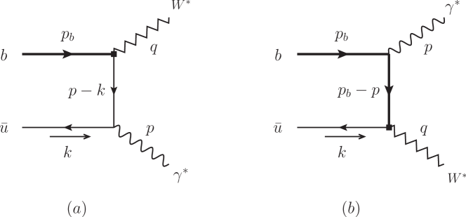
Figure 1: Diagrammatical representation of the QCD correlation function $T_{\nu\mu}(p_{B},q)$ at LO in the strong coupling constant.

Following the computational strategy detailed in [12], we start with the tree-level contribution to the QCD correlation function (4) from the diagram 1(a)

$$T_{\nu\mu}(p,q) \supset i\,Q_{u}\,\int d^{4}x\,\int{d^{4}k\over(2\,\pi)^{4}}\,{\rm exp}\left(i\,k\cdot x\right)\,{1\over(p-k)^{2}+i0}$$ (36)

$$\times\,\left\langle 0\left|\bar{u}(x)\,\gamma_{\nu}\,(\not\!p-\not\!k)\,\gamma_{\mu}\,(1-\gamma_{5})\,h_{v}(0)\right|B^{-}_{u}(v)\right\rangle\,.$$

Expanding the hard-collinear quark propagator appeared in (36) at the next-to-leading-power (NLP) accuracy leads to

$${\not\!p\,-\not\!k\over(p-k)^{2}} = \underbrace{{1\over\bar{n}\cdot(p-k)}\,{\not\!{\bar{n}}\over 2}}\,\,+\,\underbrace{\left\{{n\cdot k\,\,\bar{n}\cdot k\over n\cdot p\,\left[\bar{n}\cdot(p-k)\right]^{2}}\,{\not\!{\bar{n}}\over 2}\,+{1\over n\cdot p}\,{\not\!n\over 2}\,-{\not\!k_{\perp}\over n\cdot p\,\bar{n}\cdot(p-k)}\right\}}+...\,,\hskip 28.45274pt$$

$$\hskip 28.45274pt{\rm LP}\hskip 165.02606pt{\rm NLP}$$

where the abbreviation “${\rm LP}$” stands for the leading power term in the heavy quark expansion. The yielding NLP correction from the first non-local term in curly brackets can be computed with the well-known operator identity [39, 40]

$$v_{\mu}\,{\partial\over\partial x_{\mu}}\,\left[\bar{q}(x)\,\Gamma\,h_{v}(0)\right]=i\,\int_{0}^{1}du\,\bar{u}\,\bar{q}(x)\,g_{s}\,G_{\alpha\beta}(ux)\,x^{\alpha}\,v^{\beta}\,\Gamma\,h_{v}(0)+(v\cdot\partial)\,\left[\bar{q}(x)\,\Gamma\,h_{v}(0)\right],$$ (38)

due to the HQET equations of motion at the classical level (see [41, 42] for further discussions). Moreover, it proves necessary to implement the improved parametrization of the vacuum-to-$B$-meson matrix element of the three-body quark-gluon operator [43]

$$\langle 0|\bar{q}_{\alpha}(\tau_{1}\,n)\,g_{s}\,G_{\mu\nu}(\tau_{2}\,n)\,h_{v\,\beta}(0)|\bar{B}_{q}(v)\rangle$$

$$={\tilde{f}_{B_{q}}(\mu)\,m_{B_{q}}\over 4}\,\bigg{[}(1+\not{v})\,\bigg{\{}(v_{\mu}\gamma_{\nu}-v_{\nu}\gamma_{\mu})\,\left[\Psi_{A}(\tau_{1},\tau_{2},\mu)-\Psi_{V}(\tau_{1},\tau_{2},\mu)\right]-i\,\sigma_{\mu\nu}\,\Psi_{V}(\tau_{1},\tau_{2},\mu)$$

$$\hskip 11.38092pt-(n_{\mu}\,v_{\nu}-n_{\nu}\,v_{\mu})\,X_{A}(\tau_{1},\tau_{2},\mu)+(n_{\mu}\,\gamma_{\nu}-n_{\nu}\,\gamma_{\mu})\,\left[W(\tau_{1},\tau_{2},\mu)+Y_{A}(\tau_{1},\tau_{2},\mu)\right]$$

$$\hskip 11.38092pt+\,i\,\epsilon_{\mu\nu\alpha\beta}\,n^{\alpha}\,v^{\beta}\,\gamma_{5}\,\tilde{X}_{A}(\tau_{1},\tau_{2},\mu)-\,i\,\epsilon_{\mu\nu\alpha\beta}\,n^{\alpha}\,\gamma^{\beta}\,\gamma_{5}\,\tilde{Y}_{A}(\tau_{1},\tau_{2},\mu)$$

$$\hskip 11.38092pt-\,(n_{\mu}\,v_{\nu}-n_{\nu}\,v_{\mu})\,\not{n}\,W(\tau_{1},\tau_{2},\mu)+\,(n_{\mu}\,\gamma_{\nu}-n_{\nu}\,\gamma_{\mu})\,\not{n}\,Z(\tau_{1},\tau_{2},\mu)\bigg{\}}\,\gamma_{5}\bigg{]}_{\beta\,\alpha}\,.$$ (39)

Apparently, the relevant momentum-space distribution amplitudes can be obtained by performing the Fourier transformation with respect to the light-cone variables $\tau_{1}$ and $\tau_{2}$

$$\Psi_{X}(\tau_{1},\,\tau_{2},\,\mu)=\int_{0}^{\infty}\,d\omega_{1}\,\int_{0}^{\infty}\,d\omega_{2}\,e^{-i\,(\omega_{1}\,\tau_{1}+\omega_{2}\,\tau_{2})}\,\,\psi_{X}(\omega_{1},\omega_{2},\mu)\,,$$

$$\Psi_{X}\in\left\{\Psi_{V},\,\Psi_{A},\,X_{A},\,Y_{A},\,\tilde{X}_{A},\,\tilde{Y}_{A},\,W,\,Z\right\}\,.$$ (40)

To facilitate the construction of the desired soft-collinear factorization formulae, we express the eight invariant functions $\Psi_{X}$ in terms of the more suitable distribution amplitudes with the definite collinear twist (see [44] for an alternative proposal of geometric twist)

$$\Phi_{3} = \Phi_{A}-\Phi_{V}\,,\qquad\hskip 108.12054pt\Phi_{4}=\Phi_{A}+\Phi_{V}\,,$$

$$\hat{\Psi}_{4} = \Psi_{A}+X_{A}\,,\qquad\hskip 108.12054pt\tilde{\Psi}_{4}=\Psi_{V}-\tilde{X}_{A}\,,$$

$$\tilde{\Phi}_{5} = \Psi_{A}+\Psi_{V}+2\,Y_{A}-2\,\tilde{Y}_{A}+2\,W\,,\qquad\Psi_{5}=-\Psi_{A}+X_{A}-2\,Y_{A}\,,$$

$$\tilde{\Psi}_{5} = -\Psi_{V}-\tilde{X}_{A}+2\,\tilde{Y}_{A}\,,\qquad\hskip 62.59596pt\Phi_{6}=\Phi_{A}-\Phi_{V}+2\,Y_{A}+2\,W+2\,\tilde{Y}_{A}-4\,Z\,.\hskip 28.45274pt$$ (41)

We can then readily obtain the factorized expression for such NLP contribution

$$T_{\nu\mu,\,{\rm NLP}}^{\rm hc,\,(I)}(p,q)=-\frac{Q_{u}\,\tilde{f}_{B}(\mu)\,m_{B}}{n\cdot p}\,\left[\left(g^{\perp}_{\mu\nu}-i\,\epsilon_{\mu\nu nv}\right)\,\mathcal{G}_{\rm NLP,\,L}^{\rm hc,\,(I)}+\bar{n}_{\mu}\bar{n}_{\nu}\,\mathcal{G}_{{\rm NLP},\,\bar{n}\,\bar{n}}^{\rm hc,\,(I)}\right]\,,$$ (42)

where the newly defined “form factors” $\mathcal{G}_{X}^{\rm hc,\,(I)}$ are given by

$$\mathcal{G}_{\rm NLP,\,L}^{\rm hc,\,(I)} = \int^{\infty}_{0}d\omega_{1}\,\int^{\infty}_{0}d\omega_{2}\,\int^{1}_{0}du\,\,\frac{\bar{u}\,(\bar{n}\cdot p+\omega_{1}+u\,\omega_{2})}{(\bar{n}\cdot p-\omega_{1}-u\,\omega_{2})^{3}}\,\psi_{4}(\omega_{1},\omega_{2},\mu)$$ (43)

$$+\int^{\infty}_{0}d\omega\,\frac{\omega}{(\bar{n}\cdot p-\omega)^{2}}\,\left(\bar{\Lambda}-\frac{\omega}{2}\right)\,\phi_{B}^{+}(\omega,\mu)\,,$$

$$\mathcal{G}_{{\rm NLP},\,\bar{n}\,\bar{n}}^{\rm hc,\,(I)} = \int^{\infty}_{0}d\omega_{1}\,\int^{\infty}_{0}d\omega_{2}\,\int^{1}_{0}du\,\,\frac{\bar{u}\,(\bar{n}\cdot p+\omega_{1}+u\,\omega_{2})}{(\bar{n}\cdot p-\omega_{1}-u\,\omega_{2})^{3}}\,\psi_{5}(\omega_{1},\omega_{2},\mu)$$ (44)

$$+\int^{\infty}_{0}d\omega\,\frac{\omega}{(\bar{n}\cdot p-\omega)^{2}}\,\left(\bar{\Lambda}-\frac{\omega}{2}\right)\,\phi_{B}^{-}(\omega,\mu)\,.$$

The hadronic parameter $\bar{\Lambda}$ entering (43) and (44)can be defined in a manifestly covariant and gauge invariant manner [45]

$$\bar{\Lambda}=\frac{\langle 0|\bar{q}\,\,i\,v\cdot\overleftarrow{D}\,\Gamma\,h_{v}|\bar{B}_{q}(v)\rangle}{\langle 0|\bar{q}\,\Gamma\,h_{v}|\bar{B}_{q}(v)\rangle}\,.$$ (45)

The subleading power contribution from the second local term in curly brackets of (3.2) can be evidently expressed by the $B$-meson decay constant

$$T_{\nu\mu,\,{\rm NLP}}^{\rm hc,\,(II)}(p,q)=-\frac{Q_{u}\,\tilde{f}_{B}(\mu)\,m_{B}}{2\,n\cdot p}\,\left[\left(g^{\perp}_{\mu\nu}+i\,\epsilon_{\mu\nu nv}\right)\,-n_{\mu}n_{\nu}\right]\,.$$ (46)

Applying an additional HQET operator identity from the equations of motion

$${\partial\over\partial x_{\rho}}\bar{q}(x)\,\gamma_{\rho}\,\Gamma\,h_{v}(0) = -i\,\int_{0}^{1}du\,u\,\,\bar{q}(x)\,g_{s}\,G^{\lambda\rho}(ux)\,x_{\lambda}\,\gamma_{\rho}\,\Gamma\,h_{v}(0)\,,$$ (47)

we can proceed to construct the tree-level factorization formula for the third non-local term in curly brackets of (3.2)

$$T_{\nu\mu,\,{\rm NLP}}^{\rm hc,\,(III)}(p,q)=\frac{Q_{u}\,\tilde{f}_{B}(\mu)\,m_{B}}{n\cdot p}\,\left[{\bar{n}}_{\mu}n_{\nu}\,\mathcal{G}_{{\rm NLP},\,\bar{n}\,n}^{\rm hc,\,(III)}+{n}_{\mu}\bar{n}_{\nu}\,\mathcal{G}_{{\rm NLP},\,n\,\bar{n}}^{\rm hc,\,(III)}\right]\,,$$ (48)

where

$$\mathcal{G}_{{\rm NLP},\,\bar{n}\,n}^{\rm hc,\,(III)} = -\int^{\infty}_{0}d\omega\,\frac{\omega}{\bar{n}\cdot p-\omega}\,{\phi_{B}^{-}(\omega,\mu)\over 2}-\int^{\infty}_{0}d\omega_{1}\,\int^{\infty}_{0}d\omega_{2}\,\int^{1}_{0}du\,\,\frac{u\,\phi_{3}(\omega_{1},\omega_{2},\mu)}{(\bar{n}\cdot p-\omega_{1}-u\,\omega_{2})^{2}}\,,\hskip 22.76228pt$$ (49)

$$\mathcal{G}_{{\rm NLP},\,n\,\bar{n}}^{\rm hc,\,(III)} = -\int^{\infty}_{0}d\omega_{1}\,\int^{\infty}_{0}d\omega_{2}\,\int^{1}_{0}du\,\,\frac{1}{(\bar{n}\cdot p-\omega_{1}-u\,\omega_{2})^{2}}\,\left[u\,\phi_{4}(\omega_{1},\omega_{2},\mu)+\psi_{4}(\omega_{1},\omega_{2},\mu)\right]$$ (50)

$$-\int^{\infty}_{0}d\omega\,\frac{1}{\bar{n}\cdot p-\omega}\,\left(\bar{\Lambda}-{\omega\over 2}\right)\,\phi_{B}^{+}(\omega,\mu)\,.$$

Adding the different pieces together, the “dynamical” power corrections to the exclusive $B_{u}^{-}\to\gamma^{\ast}\,\ell\,\bar{\nu}_{\ell}$ form factors due to the energetic photon emission from the light quark can be summarized in the following

$$F_{V,\,{\rm NLP}}^{\rm hc,\,dyn} = -\frac{2\,Q_{u}\,\tilde{f}_{B}(\mu)\,m_{B}}{(n\cdot p)^{2}}\,\left(\mathcal{G}_{\rm NLP,\,L}^{\rm hc,\,(I)}-{1\over 2}\right)+{\cal O}\left(\alpha_{s},\,{\Lambda/m_{b}}\right)\,,$$

$$\hat{F}_{A,\,{\rm NLP}}^{\rm hc,\,dyn} = -\frac{2\,Q_{u}\,\tilde{f}_{B}(\mu)\,m_{B}}{(n\cdot p)^{2}}\,\left(\mathcal{G}_{\rm NLP,\,L}^{\rm hc,\,(I)}+{1\over 2}\right)+{\cal O}\left(\alpha_{s},\,{\Lambda/m_{b}}\right)\,,$$

$$\hat{F}_{1,\,{\rm NLP}}^{\rm hc,\,dyn} = \frac{4\,Q_{u}\,\tilde{f}_{B}(\mu)\,m_{B}}{(n\cdot p)^{2}}\,\left(\mathcal{G}_{{\rm NLP},\,\bar{n}\,n}^{\rm hc,\,(III)}-{1\over 2}\right)+{\cal O}\left(\alpha_{s},\,{\Lambda/m_{b}}\right)\,,$$

$$\hat{F}_{2,\,{\rm NLP}}^{\rm hc,\,dyn} = \frac{4\,Q_{u}\,\tilde{f}_{B}(\mu)\,m_{B}}{(n\cdot p)^{2}}\,\left(\mathcal{G}_{{\rm NLP},\,n\,\bar{n}}^{\rm hc,\,(III)}-{1\over 2}\right)+{\cal O}\left(\alpha_{s},\,{\Lambda/m_{b}}\right)\,,$$

$$\hat{F}_{3,\,{\rm NLP}}^{\rm hc,\,dyn} = \frac{4\,Q_{u}\,\tilde{f}_{B}(\mu)\,m_{B}}{(n\cdot p)^{2}}+{\cal O}\left(\alpha_{s},\,{\Lambda/m_{b}}\right)\,,$$

$$\hat{F}_{4,\,{\rm NLP}}^{\rm hc,\,dyn} = \frac{2\,Q_{u}\,\tilde{f}_{B}(\mu)\,m_{B}}{(n\cdot p)^{2}}\,\left(\mathcal{G}_{{\rm NLP},\,\bar{n}\,\bar{n}}^{\rm hc,\,(I)}-\mathcal{G}_{{\rm NLP},\,\bar{n}\,n}^{\rm hc,\,(III)}-\mathcal{G}_{{\rm NLP},\,n\,\bar{n}}^{\rm hc,\,(III)}+{1\over 2}\right)+{\cal O}\left(\alpha_{s},\,{\Lambda/m_{b}}\right)\,.$$ (51)

We are now in a position to compute the subleading power corrections to the radiative $B_{u}^{-}\to\gamma^{\ast}\,\ell\,\bar{\nu}_{\ell}$ form factors from both the two-particle and three-particle $B$-meson distribution amplitudes at tree level by employing the perturbative factorization technique. Implementing the light-cone expansion of the hard-collinear quark propagator in the background soft-gluon field [46] (see [47] for an improved discussion on the massive quark propagator)

$$\langle 0|{\rm T}\,\{\bar{q}(x),q(0)\}|0\rangle\supset i\,g_{s}\,\int_{0}^{\infty}\,\,{d^{4}\ell\over(2\pi)^{4}}\,{e^{-i\,\ell\cdot x}\over\ell^{2}-m_{q}^{2}}\,\int_{0}^{1}\,du\,\left[u\,x_{\mu}\,\gamma_{\nu}-\frac{(\not{\ell}+m_{q})\,\sigma_{\mu\nu}}{2\,\left(\ell^{2}-m_{q}^{2}\right)}\right]\,G^{\mu\nu}(u\,x)\,,\hskip 17.07182pt$$ (52)

with the gluon-field strength tensor $G^{\mu\nu}=G_{\mu\nu}^{a}\,T^{a}=D_{\mu}\,A_{\nu}-D_{\nu}\,A_{\mu}$, and taking advantage of the general parametrization of the three-body HQET matrix element (39), we can immediately establish the soft-collinear factorization formulae for the three-particle higher twist corrections

$$F_{V,\,{\rm NLP}}^{\rm 3PHT} = \hat{F}_{A,\,{\rm NLP}}^{\rm 3PHT}=\frac{Q_{u}\,\tilde{f}_{B}(\mu)\,m_{B}}{(n\cdot p)^{2}}\,\int^{\infty}_{0}\,d\omega_{1}\int^{\infty}_{0}\,d\omega_{2}\,\int^{1}_{0}du\,\frac{1}{(\bar{n}\cdot p-\omega_{1}-u\,\omega_{2})^{2}}$$

$$\times\,\left[(2u-1)\,\psi_{4}(\omega_{1},\omega_{2},\mu)-\tilde{\psi}_{4}(\omega_{1},\omega_{2},\mu)\right]+{\cal O}\left(\alpha_{s},\,{\Lambda/m_{b}}\right)\,,$$

$$\hat{F}_{1,\,{\rm NLP}}^{\rm 3PHT} = \frac{4\,Q_{u}\,\tilde{f}_{B}(\mu)\,m_{B}}{(n\cdot p)^{2}}\,\int^{\infty}_{0}\,d\omega_{1}\int^{\infty}_{0}\,d\omega_{2}\,\int^{1}_{0}du\,\frac{u\,\phi_{3}(\omega_{1},\omega_{2},\mu)}{(\bar{n}\cdot p-\omega_{1}-u\,\omega_{2})^{2}}+{\cal O}\left(\alpha_{s},\,{\Lambda/m_{b}}\right)\,,$$

$$\hat{F}_{2,\,{\rm NLP}}^{\rm 3PHT} = -\frac{4\,Q_{u}\,\tilde{f}_{B}(\mu)\,m_{B}}{(n\cdot p)^{2}}\,\int^{\infty}_{0}\,d\omega_{1}\int^{\infty}_{0}\,d\omega_{2}\,\int^{1}_{0}du\,\frac{(1-u)\,\phi_{4}(\omega_{1},\omega_{2},\mu)}{(\bar{n}\cdot p-\omega_{1}-u\,\omega_{2})^{2}}+{\cal O}\left(\alpha_{s},\,{\Lambda/m_{b}}\right)\,,$$

$$\hat{F}_{3,\,{\rm NLP}}^{\rm 3PHT} = {\cal O}\left(\alpha_{s},\,{\Lambda/m_{b}}\right)\,,$$

$$\hat{F}_{4,\,{\rm NLP}}^{\rm 3PHT} = \frac{2\,Q_{u}\,\tilde{f}_{B}(\mu)\,m_{B}}{(n\cdot p)^{2}}\,\,\int^{\infty}_{0}\,d\omega_{1}\int^{\infty}_{0}\,d\omega_{2}\,\int^{1}_{0}du\,\frac{1}{(\bar{n}\cdot p-\omega_{1}-u\,\omega_{2})^{2}}\,\Big{[}(1-2u)\,\psi_{5}(\omega_{1},\omega_{2},\mu)$$ (53)

$$+\,\tilde{\psi}_{5}(\omega_{1},\omega_{2},\mu)+(1-u)\,\phi_{4}(\omega_{1},\omega_{2},\mu)-u\,\phi_{3}(\omega_{1},\omega_{2},\mu)\Big{]}+{\cal O}\left(\alpha_{s},\,{\Lambda/m_{b}}\right)\,,$$

where the achieved expressions for the two form factors $F_{V,\,{\rm NLP}}^{\rm 3PHT}$ and $F_{A,\,{\rm NLP}}^{\rm 3PHT}$ are in accordance with the analogous NLP contributions to the double radiative bottom-meson decays in the kinematic limit $\bar{n}\cdot p\to 0$ as displayed in Eq. (4.37) in [12].

For the purpose of evaluating the two-particle higher-twist effects, we will introduce the generalized decomposition of the two-body non-local $B$-meson-to-vacuum matrix element with the off-light-cone corrections up to the ${\cal O}(x^{2})$ accuracy [43]

$$\langle 0|(\bar{q}_{s}Y_{s})_{\beta}(x)\,\,\,(Y_{s}^{{\dagger}}h_{v})_{\alpha}(0)|\bar{B}_{q}\rangle$$

$$=-{i\,\tilde{f}_{B_{q}}(\mu)\,m_{B_{q}}\over 4}\,\int_{0}^{\infty}d\omega\,e^{-i\omega v\cdot x}\,\bigg{[}{1+\not{v}\over 2}\,\bigg{\{}2\,\left[\phi_{B}^{+}(\omega,\mu)+x^{2}\,g_{B}^{+}(\omega,\mu)\right]$$

$$\hskip 14.22636pt\,-{\not{x}\over v\cdot x}\,\left[(\phi_{B}^{+}(\omega,\mu)-\phi_{B}^{-}(\omega,\mu))+x^{2}\,(g_{B}^{+}(\omega,\mu)-g_{B}^{-}(\omega,\mu))\right]\,\bigg{\}}\,\gamma_{5}\bigg{]}_{\alpha\beta}\,.$$ (54)

It is then straightforward to write down the resulting factorized expression

$$T_{\nu\mu}^{\rm 2PHT}(p,q) = -\frac{2\,Q_{u}\,\tilde{f}_{B}(\mu)\,m_{B}}{n\cdot p}\,\bigg{\{}\left(g_{\mu\nu}^{\perp}-i\,\epsilon_{\mu\nu\rho\sigma}\,n^{\rho}\,v^{\sigma}\right)\,\int^{\infty}_{0}\,d\omega\,\frac{g_{B}^{+}(\omega,\mu)}{(\bar{n}\cdot p-\omega)^{2}}\,$$ (55)

$$-\,\bar{n}_{\mu}\,\bar{n}_{\nu}\,\int^{\infty}_{0}d\omega\,\frac{g_{B}^{-}(\omega,\mu)}{(\bar{n}\cdot p-\omega)^{2}}\bigg{\}}\,.$$

Applying the two non-trivial constraints on the subleading twist HQET distribution amplitudes in momentum space [14, 16] (see also [39, 40, 43] for the coordinate-space identities)

$$-2\,{d^{2}\over d\omega^{2}}\,g_{B}^{+}(\omega,\mu) = \left[{3\over 2}+(\omega-\bar{\Lambda})\,{d\over d\omega}\right]\,\phi_{B}^{+}(\omega,\mu)-{1\over 2}\,\phi_{B}^{-}(\omega,\mu)+\int_{0}^{\infty}\,{d\omega_{2}\over\omega_{2}}\,{d\over d\omega}\,\psi_{4}(\omega,\omega_{2},\mu)$$ (56)

$$-\int_{0}^{\infty}\,{d\omega_{2}\over\omega_{2}^{2}}\,\psi_{4}(\omega,\omega_{2},\mu)+\int_{0}^{\omega}\,{d\omega_{2}\over\omega_{2}^{2}}\,\psi_{4}(\omega-\omega_{2},\omega_{2},\mu)\,,$$

$$-2\,{d^{2}\over d\omega^{2}}\,g_{B}^{-}(\omega,\mu) = \left[{3\over 2}+(\omega-\bar{\Lambda})\,{d\over d\omega}\right]\,\phi_{B}^{-}(\omega,\mu)-{1\over 2}\,\phi_{B}^{+}(\omega,\mu)+\int_{0}^{\infty}\,{d\omega_{2}\over\omega_{2}}\,{d\over d\omega}\,\psi_{5}(\omega,\omega_{2},\mu)$$ (57)

$$-\int_{0}^{\infty}\,{d\omega_{2}\over\omega_{2}^{2}}\,\psi_{5}(\omega,\omega_{2},\mu)+\int_{0}^{\omega}\,{d\omega_{2}\over\omega_{2}^{2}}\,\psi_{5}(\omega-\omega_{2},\omega_{2},\mu)\,,$$

the twist-four and twist-five $B$-meson distribution amplitudes $g_{B}^{\pm}(\omega,\mu)$ can be decomposed into the Wandzura-Wilczek contributions [48] calculable from the lower-twist two-particle distribution amplitudes $\phi_{B}^{\pm}(\omega,\mu)$ and the “genuine” three-particle distribution amplitudes of the same collinear twists

$$g_{B}^{+}(\omega,\mu) = \hat{g}_{B}^{+}(\omega,\mu)-{1\over 2}\,\int_{0}^{\omega}\,d\omega_{1}\,\int_{0}^{1}du\,{\bar{u}\over u}\,\,\psi_{4}\left(\omega,{\omega-\omega_{1}\over u},\mu\right)\,,$$

$$g_{B}^{-}(\omega,\mu) = \hat{g}_{B}^{-}(\omega,\mu)-{1\over 2}\,\int_{0}^{\omega}\,d\omega_{1}\,\int_{0}^{1}du\,{\bar{u}\over u}\,\,\psi_{5}\left(\omega,{\omega-\omega_{1}\over u},\mu\right)\,,$$ (58)

where the manifest expressions of the Wandzura-Wilczek terms are given by

$$\hat{g}_{B}^{+}(\omega,\mu) = {1\over 4}\,\int_{\omega}^{\infty}\,d\rho\,\bigg{\{}(\rho-\omega)\,\left[\phi_{B}^{-}(\rho,\mu)-\phi_{B}^{+}(\rho,\mu)\right]-2\,(\bar{\Lambda}-\rho)\,\phi_{B}^{+}(\rho,\mu)\bigg{\}}\,,$$

$$\hat{g}_{B}^{-}(\omega,\mu) = {1\over 4}\,\int_{\omega}^{\infty}\,d\rho\,\bigg{\{}(\rho-\omega)\,\left[\phi_{B}^{+}(\rho,\mu)-\phi_{B}^{-}(\rho,\mu)\right]-2\,(\bar{\Lambda}-\rho)\,\phi_{B}^{-}(\rho,\mu)\bigg{\}}\,.$$ (59)

We are then led to an equivalent form of the obtained factorization formula (55)

$$T_{\nu\mu}^{\rm 2PHT}(p,q) = -\frac{Q_{u}\,\tilde{f}_{B}(\mu)\,m_{B}}{n\cdot p}\,\bigg{\{}\left(g_{\mu\nu}^{\perp}-i\,\epsilon_{\mu\nu\rho\sigma}\,n^{\rho}\,v^{\sigma}\right)\,{\cal G}_{\rm NLP,\,L}^{\rm 2PHT}+\,\bar{n}_{\mu}\,\bar{n}_{\nu}\,\,{\cal G}_{{\rm NLP},\,\bar{n}\,\bar{n}}^{\rm 2PHT}\bigg{\}}\,,$$ (60)

where the newly introduced invariant functions are defined as follows

$${\cal G}_{\rm NLP,\,L}^{\rm 2PHT} = 2\,\int^{\infty}_{0}\,d\omega\,\frac{\hat{g}_{B}^{+}(\omega,\mu)}{(\bar{n}\cdot p-\omega)^{2}}-\int^{\infty}_{0}\,d\omega_{1}\int^{\infty}_{0}\,d\omega_{2}\,\int^{1}_{0}du\,\frac{(1-u)\,\psi_{4}(\omega_{1},\omega_{2},\mu)}{(\bar{n}\cdot p-\omega_{1}-u\,\omega_{2})^{2}}\,,$$

$${\cal G}_{{\rm NLP},\,\bar{n}\,\bar{n}}^{\rm 2PHT} = -2\,\int^{\infty}_{0}\,d\omega\,\frac{\hat{g}_{B}^{-}(\omega,\mu)}{(\bar{n}\cdot p-\omega)^{2}}+\int^{\infty}_{0}\,d\omega_{1}\int^{\infty}_{0}\,d\omega_{2}\,\int^{1}_{0}du\,\frac{(1-u)\,\psi_{5}(\omega_{1},\omega_{2},\mu)}{(\bar{n}\cdot p-\omega_{1}-u\,\omega_{2})^{2}}\,.\hskip 14.22636pt$$ (61)

Matching the tree-level SCET computation of the correlation function $T_{\nu\mu}$ (60) onto the appropriate hadronic representation (12) yields

$$F_{V,\,{\rm NLP}}^{\rm 2PHT} = \hat{F}_{A,\,{\rm NLP}}^{\rm 2PHT}=-\frac{2\,Q_{u}\,\tilde{f}_{B}(\mu)\,m_{B}}{(n\cdot p)^{2}}\,{\cal G}_{\rm NLP,\,L}^{\rm 2PHT}+{\cal O}\left(\alpha_{s},\,{\Lambda/m_{b}}\right)\,,$$

$$\hat{F}_{1,\,{\rm NLP}}^{\rm 2PHT} = {\cal O}\left(\alpha_{s},\,{\Lambda/m_{b}}\right)\,,$$

$$\hat{F}_{2,\,{\rm NLP}}^{\rm 2PHT} = {\cal O}\left(\alpha_{s},\,{\Lambda/m_{b}}\right)\,,$$

$$\hat{F}_{3,\,{\rm NLP}}^{\rm 2PHT} = {\cal O}\left(\alpha_{s},\,{\Lambda/m_{b}}\right)\,,$$

$$\hat{F}_{4,\,{\rm NLP}}^{\rm 2PHT} = -\frac{2\,Q_{u}\,\tilde{f}_{B}(\mu)\,m_{B}}{(n\cdot p)^{2}}\,{\cal G}_{{\rm NLP},\,\bar{n}\,\bar{n}}^{\rm 2PHT}+{\cal O}\left(\alpha_{s},\,{\Lambda/m_{b}}\right)\,,$$ (62)

where the factorized expression of $F_{V,\,{\rm NLP}}^{\rm 2PHT}$ ($\hat{F}_{A,\,{\rm NLP}}^{\rm 2PHT}$) can be alternatively inferred from the two-particle subleading twist correction to $B_{u}^{-}\to\gamma\,\ell\,\bar{\nu}_{\ell}$ [8] and the established formula of $\hat{F}_{4,\,{\rm NLP}}^{\rm 2PHT}$ is completely consistent with the counterpart contribution to the very correlation function suitable for constructing the light-cone QCD sum rules for $B\to\pi,K$ form factors [15].

The “kinematic” power corrections to the radiative $B$-meson decay form factors can be determined by employing an equivalent hadronic representation for the correlation function $T_{\nu\mu}$ other than (8) and (12)

$$T_{\nu\mu}(p,q) = {n\cdot p\over 2}\,\left[-i\,(1-\kappa_{p})\epsilon_{\mu\nu\rho\sigma}\,n^{\rho}\,v^{\sigma}\,F_{V}+(1+\kappa_{p})\,g_{\mu\nu}^{\perp}\,\hat{F}_{A}\right]$$ (63)

$$+{n\cdot p\over 4}\,\left[\left(\hat{F}_{1}+\frac{\hat{F}_{3}}{2}\right)+\kappa_{p}\,\left(\hat{F}_{2}+\frac{\hat{F}_{3}}{2}+2\,\hat{F}_{4}\right)\right]\,\bar{n}_{\mu}\,n_{\nu}$$

$$+{n\cdot p\over 4}\,\left[\left(\hat{F}_{2}+\frac{\hat{F}_{3}}{2}\right)+\kappa_{p}\,\left(\hat{F}_{1}+\frac{\hat{F}_{3}}{2}+2\,\hat{F}_{4}\right)\right]\,n_{\mu}\,{\bar{n}}_{\nu}$$

$$+{n\cdot p\over 4}\,\left[\left(\hat{F}_{1}+\hat{F}_{2}+\frac{\hat{F}_{3}}{2}+2\,\hat{F}_{4}\right)+\kappa_{p}\,\left(\frac{\hat{F}_{3}}{2}-2\,\hat{F}_{4}\right)\right]\,{\bar{n}}_{\mu}\,{\bar{n}}_{\nu}$$

$$+{n\cdot p\over 4}\,\left[\frac{\hat{F}_{3}}{2}+\kappa_{p}\,\left(\hat{F}_{1}+\hat{F}_{2}+\frac{\hat{F}_{3}}{2}\right)\right]\,n_{\mu}\,n_{\nu}+{\cal O}(\kappa_{p}^{2})\,,$$

where the dimensionless variable $\kappa_{p}$ is explicitly defined by

$$\kappa_{p}\equiv{p^{2}\over(n\cdot p)^{2}}\sim{\cal O}\left({\Lambda_{\rm QCD}\over m_{b}}\right)\,.$$ (64)

Confronting (63) with the LP QCD expression for the diagram 1(a) allows for the determination of the subleading power “kinematic” corrections at tree level

$$F_{V,\,{\rm NLP}}^{\rm hc,\,kin} = -\kappa_{p}\,\frac{Q_{u}\,\tilde{f}_{B}(\mu)\,m_{B}}{n\cdot p}\,\int^{\infty}_{0}\,\frac{d\omega}{\bar{n}\cdot p-\omega}\,\phi_{B}^{+}(\omega,\mu)+{\cal O}\left(\alpha_{s},\,\kappa_{p}^{2}\right)\,,$$

$$\hat{F}_{A,\,{\rm NLP}}^{\rm hc,\,kin} = \kappa_{p}\,\frac{Q_{u}\,\tilde{f}_{B}(\mu)\,m_{B}}{n\cdot p}\,\int^{\infty}_{0}\,\frac{d\omega}{\bar{n}\cdot p-\omega}\,\phi_{B}^{+}(\omega,\mu)+{\cal O}\left(\alpha_{s},\,\kappa_{p}^{2}\right)\,,$$

$$\hat{F}_{1,\,{\rm NLP}}^{\rm hc,\,kin} = -2\,\kappa_{p}\,\frac{Q_{u}\,\tilde{f}_{B}(\mu)\,m_{B}}{n\cdot p}\,\int^{\infty}_{0}\,\frac{d\omega}{\bar{n}\cdot p-\omega}\,\phi_{B}^{-}(\omega,\mu)+{\cal O}\left(\alpha_{s},\,\kappa_{p}^{2}\right)\,,$$

$$\hat{F}_{2,\,{\rm NLP}}^{\rm hc,\,kin} = -2\,\kappa_{p}\,\frac{Q_{u}\,\tilde{f}_{B}(\mu)\,m_{B}}{n\cdot p}\,\int^{\infty}_{0}\,\frac{d\omega}{\bar{n}\cdot p-\omega}\,\phi_{B}^{-}(\omega,\mu)+{\cal O}\left(\alpha_{s},\,\kappa_{p}^{2}\right)\,,$$

$$\hat{F}_{3,\,{\rm NLP}}^{\rm hc,\,kin} = {\cal O}\left(\alpha_{s},\,\kappa_{p}^{2}\right)\,,$$

$$\hat{F}_{4,\,{\rm NLP}}^{\rm hc,\,kin} = 3\,\kappa_{p}\,\frac{Q_{u}\,\tilde{f}_{B}(\mu)\,m_{B}}{n\cdot p}\,\int^{\infty}_{0}\,\frac{d\omega}{\bar{n}\cdot p-\omega}\,\phi_{B}^{-}(\omega,\mu)+{\cal O}\left(\alpha_{s},\,\kappa_{p}^{2}\right)\,.$$ (65)

Furthermore, we derive the power suppressed local contribution from the hard-collinear photon radiation off the bottom quark as displayed in the diagram 1(b)

$$F_{V,\,\rm NLP}^{Q_{b},\,\rm loc} = -\frac{\tilde{f}_{B}(\mu)\,m_{B}}{\overline{m}^{2}_{b}}\,\frac{Q_{b}}{r_{3}-1}\,+{\cal O}\left(\alpha_{s},\,{\Lambda/m_{b}}\right)\,,$$

$$\hat{F}_{A,\,\rm NLP}^{Q_{b},\,\rm loc} = \frac{\tilde{f}_{B}(\mu)\,m_{B}}{\overline{m}^{2}_{b}}\,\left(1+2\,\frac{\overline{y_{B}}}{r_{1}}\right)\,\frac{Q_{b}}{r_{3}-1}\,+{\cal O}\left(\alpha_{s},\,{\Lambda/m_{b}}\right)\,,$$

$$\hat{F}_{1,\,\rm NLP}^{Q_{b},\,\rm loc} = \frac{4\,\tilde{f}_{B}(\mu)\,m_{B}}{\overline{m}^{2}_{b}}\,\left({r_{2}\over r_{1}^{2}}+\frac{\overline{y_{B}}}{2\,r_{1}}\right)\,\frac{Q_{b}}{r_{3}-1}+{\cal O}\left(\alpha_{s},\,{\Lambda/m_{b}}\right)\,,$$

$$\hat{F}_{2,\,\rm NLP}^{Q_{b},\,\rm loc} = \frac{4\,\tilde{f}_{B}(\mu)\,m_{B}}{\overline{m}^{2}_{b}}\,\left({r_{2}\over r_{1}^{2}}+\frac{\overline{y_{B}}}{2\,r_{1}}\right)\,\frac{Q_{b}}{r_{3}-1}+{\cal O}\left(\alpha_{s},\,{\Lambda/m_{b}}\right)\,,$$

$$\hat{F}_{3,\,\rm NLP}^{Q_{b},\,\rm loc} = \frac{4\,\tilde{f}_{B}(\mu)\,m_{B}}{\overline{m}^{2}_{b}}\,\frac{y_{B}}{r_{1}}\,\frac{Q_{b}}{r_{3}-1}+{\cal O}\left(\alpha_{s},\,{\Lambda/m_{b}}\right)\,,$$

$$\hat{F}_{4,\,\rm NLP}^{Q_{b},\,\rm loc} = -\frac{\tilde{f}_{B}(\mu)\,m_{B}}{\overline{m}^{2}_{b}}\,\left(1+2\,\frac{\overline{y_{B}}}{r_{1}}\right)\,\frac{Q_{b}}{r_{3}-1}+{\cal O}\left(\alpha_{s},\,{\Lambda/m_{b}}\right)\,,$$ (66)

by introducing further three dimensionless quantities

$$y_{B}=m_{b}/\overline{m_{b}}\,,\qquad\overline{y_{B}}=1-y_{B}\,,\qquad r_{3}\equiv q^{2}/\overline{m}_{b}^{2}=r_{2}-y_{B}\,r_{1}+y^{2}_{B}\,.$$ (67)

The obtained expressions for the vector and axial-vector form factors are compatible with the counterpart contributions to the radiative leptonic $B_{u}^{-}\to\gamma\,\ell\,\bar{\nu}_{\ell}$ decay by taking the on-shell photon limit $p^{2}\to 0$ [5].

Collecting the individual NLP corrections discussed so far allows us to write down the following master formula

$${\cal F}_{i,\,\rm NLP}={\cal F}_{i,\,\rm NLP}^{\rm hc,\,dyn}+{\cal F}_{i,\,\rm NLP}^{\rm 3PHT}+{\cal F}_{i,\,\rm NLP}^{\rm 2PHT}+{\cal F}_{i,\,\rm NLP}^{\rm hc,\,kin}+{\cal F}_{i,\,\rm NLP}^{Q_{b},\,\rm loc}\,,\qquad({\cal F}_{i}=F_{V},\,\hat{F}_{A},\,\hat{F}_{1,...,4})\,,$$ (68)

where the detailed expressions of the separate terms appearing on the right-hand side can be found in (51), (53), (62), (65) and (66). Prior to concluding the explorations of factorization properties for the generalized $B_{u}^{-}\to\gamma^{\ast}\,W^{\ast}$ form factors with a hard-collinear photon, we pause for a while to compare our computations of the subleading power terms in the heavy quark expansion with the previous theory analysis in the QCD framework [49, 50, 51].

• To facilitate an exploratory comparison with [50], we first establish the conversion relation of their ${\it``longitudinal"}$ form factor $\hat{F}_{A_{\|}}$ and a complete set of the exclusive transition form factors introduced in (8)

  $$\hat{F}_{A_{\|}}=-\left[F_{1}+{v\cdot p\over m_{B}}\,F_{3}+\hat{F}_{A}\right]\,,$$ (69)

  which further implies another advantageous representation with the aid of our equation (14) as well as the two relevant identities in (2.4) and (2.6) of [50]

  $$F_{A_{\|}}=-\left\{\hat{F}_{1}+{v\cdot p\over m_{B}}\,\hat{F}_{3}+\left[1+\frac{p^{2}}{(v\cdot p)^{2}-p^{2}}\,\left(1-\frac{v\cdot p}{m_{B}}\right)\right]\,\frac{Q_{\ell}\,f_{B}}{v\cdot p}\right\}\,.$$ (70)

  Plugging the obtained NLP factorization formulae of $\hat{F}_{1}$ and $\hat{F}_{3}$ at tree level into (70) and performing the (hard)-collinear expansion up to the ${\cal O}(\Lambda_{\rm QCD}/m_{b})$ accuracy leads to

  $$F_{A_{\|}} = -\frac{4\,Q_{u}\,\tilde{f}_{B}(\mu)\,m_{B}}{(n\cdot p)^{2}}\,{\bar{n}\cdot p\over\lambda_{B}^{-}(\bar{n}\cdot p,\mu)}+{2\,\tilde{f}_{B}(\mu)\over n\cdot p}\,(Q_{b}-Q_{u}-Q_{\ell})+{\cal O}\left(\alpha_{s},\,{\Lambda_{\rm QCD}\over m_{b}}\right)\,,\hskip 28.45274pt$$ (71)

  where the second term vanishes evidently due to the electric-charge conservation and the inverse moment of the twist-three distribution amplitude $\phi_{B}^{-}(\omega,\mu)$ is defined by [10]

  $$\frac{1}{\lambda_{B}^{-}(\bar{n}\cdot p,\mu)}=\int_{0}^{\infty}\,d\omega\,{\phi_{B}^{-}(\omega,\mu)\over\omega-\bar{n}\cdot p-i\,0}\,.$$ (72)

  Interestingly, the power suppressed three-particle contribution from the “genuine” twist-three distribution amplitude $\phi_{3}(\omega_{1},\omega_{2},\mu)$ disappears at LO in the strong coupling constant, owing to the complete cancellation of the distinct dynamical mechanisms entering (51) and (53). It is straightforward to verify that the yielding expression (71) for the form factor $F_{A_{\|}}$ reproduces the obtained result of [50] adopting the Wandzura-Wilczek approximation. Inspecting the soft-collinear factorization formulae for the “dynamical” power corrections (51) reveals that the first term in the curly brackets of (3.2) will generate the non-vanishing contributions to the form factors $\hat{F}_{1}$ and $\hat{F}_{3}$ starting at next-to-next-to-leading-power (NNLP) in an expansion in powers of $\Lambda_{\rm QCD}/m_{b}$, thus supporting the proposed ansatz for the non-perturbative form factor $\xi^{\prime}(p^{2},\bar{n}\cdot p)$ [50] analytically.

• We leave out the subleading power contributions to the exclusive $B_{u}^{-}\to\gamma^{\ast}\,\ell\,\bar{\nu}_{\ell}$ decay form factors with a hard-collinear photon from the light-meson resonances (for instance $\rho$ and $\omega$) discussed in [49, 50], on account of (i) their insignificant numerical impacts in the kinematical regions satisfying the constraints $p^{2}\geq 1.5\,{\rm GeV^{2}}$ and $n\cdot p\geq 3.0\,{\rm GeV}$ as already observed in [50], (ii) particularly a lack of the rigorous and systematic formalism to address the resonance contributions. In addition, the OPE-controlled dispersion technique for evaluating the soft NLP contributions to the $\gamma^{\ast}\gamma\to\pi^{0}$ form factor [52, 53, 54] and the on-shell $B\to\gamma$ form factors cannot be straightforwardly applied to the analogous computation for the generalized $B_{u}^{-}(p_{B})\to\gamma^{\ast}(p)\,W^{\ast}(q)$ form factors in the time-like regime of $p^{2}\sim{\cal O}(\Lambda_{\rm QCD}\,m_{b})$, due to the yielding divergent dispersion integrals in the vicinity of $p^{2}=s_{0}$ with $s_{0}$ representing the threshold parameter in the $\rho$-meson channel

  $${1\over\pi}\,\int_{s_{0}}^{\infty}\,ds\,\,{{\rm Im}_{s}\,\mathcal{F}_{i}(s,n\cdot p)\over s-p^{2}-i\,0}\,,\qquad({\cal F}_{i}=F_{V},\,\hat{F}_{A},\,\hat{F}_{1,...,4})\,,$$ (73)

  which is precisely the argument to motivate an implementation of the phenomenological ansatz for the soft form factor in the so-called B-type contribution to $B_{d,\,s}\to\gamma\ell\bar{\ell}$ [11].

• Applying the principle of gauge invariance of the QED interaction, model-independent constraints on the radiative $B_{u}^{-}\to\gamma^{\ast}\,W^{\ast}$ form factors and the resulting phenomenological implications on the differential distributions for $B_{u}^{-}\to\ell^{\prime}\,\bar{\ell}^{\prime}\,\ell\,\bar{\nu}_{\ell}$ have been recently explored in [51], reaching the major observation of the vanishing form factor $F_{2A}(p^{2},n\cdot p)$ in the on-shell photon limit based upon their form-factor parametrization scheme. Switching to our form-factor convention instead implies the following relation

  $$\lim_{p^{2}\to 0}\,\left[F_{A_{\|}}+\frac{p^{2}}{(v\cdot p)^{2}-p^{2}}\,\left(1-\frac{v\cdot p}{m_{B}}\right)\,F_{A}\right]=0\,,$$ (74)

  which can be readily validated by employing the established result (71) for the transition form factor $F_{A_{\|}}$. Actually, the vanishing longitudinal form factor in the on-shell photon limit can be expected naturally from the very fact that there exists no longitudinal polarization for an on-shell photon as already mentioned in [50].

4 QCD factorization for $B_{u}^{-}\to\gamma^{\ast}\,\ell\,\bar{\nu}_{\ell}$ with a hard photon

Now we turn to derive the perturbative factorization formulae for a complete set of the $B_{u}^{-}\to\gamma^{\ast}\,W^{\ast}$ form factors with an off-shell photon state possessing the four-momentum $p_{\mu}\sim{\cal O}(m_{b})$ by implementing the ${\rm QCD\rightarrow HQET}$ matching for the $B$-meson-to-vacuum correlation function (4). Evaluating the tree-level diagrams displayed in Figure 1 at leading power in the heavy quark expansion immediately leads to the factorized expressions

$$F_{V}^{\rm LO} = -\frac{\tilde{f}_{B}(\mu)\,m_{B}}{\overline{m}^{2}_{b}}\,\left[\frac{Q_{u}}{r_{2}}+\frac{Q_{b}}{r_{3}-1}\right]+{\cal O}\left(\alpha_{s},\,{\Lambda_{\rm QCD}/m_{b}}\right)\,,$$

$$\hat{F}_{A}^{\rm LO} = -\frac{\tilde{f}_{B}(\mu)\,m_{B}}{\overline{m}^{2}_{b}}\,\left[\frac{Q_{u}}{r_{2}}-\left(1+2\,\frac{\overline{y_{B}}}{r_{1}}\right)\,\frac{Q_{b}}{r_{3}-1}\,\right]+{\cal O}\left(\alpha_{s},\,{\Lambda_{\rm QCD}/m_{b}}\right)\,,$$

$$\hat{F}_{1}^{\rm LO} = -\frac{\tilde{f}_{B}(\mu)\,m_{B}}{\overline{m}^{2}_{b}}\,\frac{4\,r_{2}}{r^{2}_{1}-4\,r_{2}}\,\left[\frac{Q_{u}}{r_{2}}-\left(1+\frac{\overline{y_{B}}\,r_{1}}{2\,r_{2}}\right)\,\frac{Q_{b}}{r_{3}-1}\,\right]+{\cal O}\left(\alpha_{s},\,{\Lambda_{\rm QCD}/m_{b}}\right)\,,$$

$$\hat{F}_{2}^{\rm LO} = -\frac{\tilde{f}_{B}(\mu)\,m_{B}}{\overline{m}^{2}_{b}}\,\frac{4\,r_{2}}{r^{2}_{1}-4\,r_{2}}\,\left[\frac{Q_{u}}{r_{2}}-\left(1+\frac{\overline{y_{B}}\,r_{1}}{2\,r_{2}}\right)\,\frac{Q_{b}}{r_{3}-1}\,\right]+{\cal O}\left(\alpha_{s},\,{\Lambda_{\rm QCD}/m_{b}}\right)\,,$$

$$\hat{F}_{3}^{\rm LO} = \frac{\tilde{f}_{B}(\mu)\,m_{B}}{\overline{m}^{2}_{b}}\,\frac{4\,r_{2}}{r^{2}_{1}-4\,r_{2}}\,\left[\frac{Q_{u}}{r_{2}}-\left(1-{y_{B}\,r_{1}\over r_{2}}+\frac{2\,(1+y_{B})}{r_{1}}\right)\,\frac{Q_{b}}{r_{3}-1}\right]+{\cal O}\left(\alpha_{s},\,{\Lambda_{\rm QCD}/m_{b}}\right)\,,$$

$$\hat{F}_{4}^{\rm LO} = \frac{\tilde{f}_{B}(\mu)\,m_{B}}{\overline{m}^{2}_{b}}\,\frac{r^{2}_{1}}{r^{2}_{1}-4\,r_{2}}\,\left[\frac{Q_{u}}{r_{2}}-\left(1+2\,\frac{\overline{y_{B}}}{r_{1}}\right)\,\frac{Q_{b}}{r_{3}-1}\right]+{\cal O}\left(\alpha_{s},\,{\Lambda_{\rm QCD}/m_{b}}\right)\,.$$ (75)

It is evident that the large-recoil symmetry relation between the vector and axial-vector form factors at $p^{2}\sim{\cal O}(m_{b}\,\Lambda_{\rm QCD})$ is no longer valid for large $p^{2}$ of order $m_{B}^{2}$ even at ${\cal O}(\alpha_{s}^{0})$, due to the emerged leading-power contribution from the hard photon radiation off the heavy bottom-quark. In addition, it is straightforward to verify that the resulting expressions of the four longitudinal form factors $\hat{F}_{1,...,4}$ satisfy the obtained Ward-Takahashi identities (16). In contrast to the SCET factorization formulae (29) for the $B_{u}^{-}\to\gamma^{\ast}\,\ell\,\bar{\nu}_{\ell}$ form factors with a hard-collinear photon, the yielding results of $\hat{F}_{1}$ and $\hat{F}_{3}$ are observed to be free of the $\Lambda_{\rm QCD}/m_{b}$ suppression compared with the remaining transition form factors at $p^{2}\sim{\cal O}(m_{b}^{2})$.

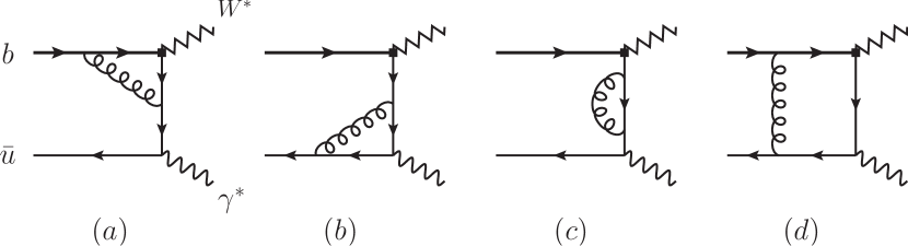
Figure 2: Diagrammatical representation of the NLO correction to the QCD correlation function $T_{\nu\mu}(p_{B},q)$ due to the hard photon radiation from the light anti-quark.

We are now in a position to perform the NLO computation of the non-local matrix element $T_{\nu\mu}(p_{B},p)$ in the hard $p^{2}$ region by applying the standard perturbative matching program, which is somewhat more sophisticated than the ${\rm QCD\rightarrow HQET}$ matching for the heavy-to-light currents at one loop [55, 45]. It is apparent that the gluonic corrections to the short-distance Wilson coefficients can be conveniently split into two pieces with the distinct electric charges in the following

$${\cal F}_{i}^{\rm NLO}={\cal F}_{i}^{\rm LO}+{\alpha_{s}(\mu)\,C_{F}\over 2\,\pi}\,\frac{\tilde{f}_{B}(\mu)\,m_{B}}{\overline{m}^{2}_{b}}\,\left[\left({Q_{u}\over r_{2}}\right)\,{\cal H}_{i}^{u}+\left({Q_{b}\over r_{3}-1}\right)\,{\cal H}_{i}^{b}\right],\,\,({\cal F}_{i}=F_{V},\,\hat{F}_{A},\,\hat{F}_{1,...,4})\,.\hskip 14.22636pt$$ (76)

The renormalized coefficient function ${\cal H}_{i}^{u}$ can be readily determined by identifying the hard contributions of the one-loop QCD diagrams presented in Figure 2 (apart from the wavefunction renormaization of the external bottom quark at ${\cal O}(\alpha_{s})$ [56])

$${\cal H}_{V}^{u} = \left(\frac{3}{4}\,\ln\frac{\mu^{2}}{m^{2}_{b}}+2\right)+\frac{1}{r_{1}^{2}-4r_{2}}\,\bigg{\{}\frac{r_{1}-4r_{2}}{2}\,r_{2}\ln(-r_{2})-\left[r_{1}^{3}+r_{2}^{2}-r_{1}\,r_{2}\,(4+r_{2})\right]\,{\cal C}_{0,\,u}$$ (77)

$$+\frac{r_{1}\,(r_{1}+3\,r_{2})-2\,r_{2}\,(3+2\,r_{2})}{2\,r_{3}}\,(1-r_{3})\,\ln(1-r_{3})\bigg{\}}\,,$$

$${\cal\hat{H}}_{A}^{u} = {\cal H}_{V}^{u}+\frac{r_{2}}{r_{1}\,(r_{1}^{2}-4r_{2})}\,\bigg{\{}2\left[r_{1}^{2}-r_{2}\,(2+r_{2})\right]\,{\cal C}_{0,\,u}+\left[r_{1}\,(r_{3}-3)+4\,r_{2}\right]\,\ln\left(-r_{2}\right)$$ (78)

$$-\frac{(r_{1}+2)\,(1-r_{3})-4}{r_{3}}\,(1-r_{3})\ln(1-r_{3})-r_{1}^{2}+4\,r_{2}\bigg{\}}\,,$$

$${\cal\hat{H}}_{1}^{u} = \frac{4\,r_{2}}{r^{2}_{1}-4r_{2}}\,\bigg{\{}\left({3\over 4}\,\ln\frac{\mu^{2}}{m^{2}_{b}}+2\right)-\,\Big{[}\frac{r_{2}}{r^{2}_{1}-4r_{2}}\,(2+r_{1}\,r_{2}-2r_{3})+r_{1}\Big{]}\,{\cal C}_{0,\,u}$$ (79)

$$+\frac{r_{3}-1}{r_{3}}\,\Big{[}\frac{2}{r^{2}_{1}-4\,r_{2}}\,(r_{2}-r^{2}_{2}+r_{1}\,r_{3})-\frac{(r_{2}-1)(r_{3}-1)}{2\,r_{3}}\Big{]}\,\ln(1-r_{3})$$

$$+\frac{r_{1}}{2\,(r^{2}_{1}-4r_{2})}\,(2+r_{1}\,r_{2}-2r_{3})\,\ln(-r_{2})+\frac{2-r_{1}-r_{1}\,r_{3}}{2\,r_{3}}\bigg{\}}\,,$$

$${\cal\hat{H}}_{2}^{u} = \left(-{r_{1}^{2}\over 4\,r_{2}}\right)\,{\cal\hat{H}}_{3}^{u}-\left({3\over 4}\,\ln\frac{\mu^{2}}{m^{2}_{b}}+1\right)\,,$$ (80)

$${\cal\hat{H}}_{3}^{u} = -\frac{4\,r_{2}}{r^{2}_{1}-4r_{2}}\,\bigg{\{}\left({3\over 4}\,\ln\frac{\mu^{2}}{m^{2}_{b}}+2\right)+\frac{2\,r_{2}}{r_{1}}\,\left[\frac{r_{2}}{r^{2}_{1}-4r_{2}}\,(-4+r_{1}-2r_{2})-2\right]\,{\cal C}_{0,\,u}$$ (81)

$$+\frac{1-r_{3}}{r_{1}\,r_{3}}\,\left[\frac{2\,r_{2}}{r^{2}_{1}-4r_{2}}\,(-4+2\,r_{1}+r_{1}\,r_{3})+\frac{(r_{2}-1)(r_{3}-1)}{r_{3}}\right]\,\ln(1-r_{3})$$

$$+\frac{r_{2}}{r_{1}}\,\left[\frac{2}{r^{2}_{1}-4r_{2}}\,(2+r_{1}\,r_{2}-2r_{3})-1\right]\,\ln(-r_{2})-\frac{2\,r_{2}\,(1+r_{3})-r_{1}}{r_{1}\,r_{3}}\bigg{\}}\,,$$

$${\cal\hat{H}}_{4}^{u} = \left(-{r_{1}^{2}\over 4\,r_{2}}\right)\,{\cal\hat{H}}_{1}^{u}\,,$$ (82)

where we have defined the perturbative loop function

$${\cal C}_{0,\,u} = \frac{1}{\sqrt{\lambda}}\,\bigg{\{}\text{Li}_{2}\left(\frac{(r_{3}+1)\sqrt{\lambda}+r_{u}}{(r_{3}-1)\sqrt{\lambda}+r_{u}}\right)+\text{Li}_{2}\left(\frac{(1+r_{3})\sqrt{\lambda}+r_{u}}{(1-r_{3})\sqrt{\lambda}+r_{u}}\right)-\text{Li}_{2}\left(\frac{(1-r_{3})\sqrt{\lambda}+r_{u}}{(r_{3}-1)\sqrt{\lambda}+r_{u}}\right)$$ (83)

$$+2\,\text{Li}_{2}\left(\frac{r_{1}-\sqrt{\lambda}}{r_{1}+\sqrt{\lambda}}\right)+2\,\text{Li}_{2}\left(1-\frac{r_{2}}{\sqrt{\lambda}}\right)+\frac{1}{2}\,\ln^{2}\left(-\frac{r_{1}+\sqrt{\lambda}}{r_{1}-\sqrt{\lambda}}\right)+\frac{\pi^{2}}{3}\bigg{\}}\,,$$

with

$$\lambda\equiv\lambda(1,r_{2},r_{3})=1+r_{2}^{2}+r_{3}^{2}-2\,r_{2}-2\,r_{3}-2\,r_{2}\,r_{3}=r_{1}^{2}-4\,r_{2}\,,$$

$$r_{u}\equiv r_{2}\,(1+r_{3})-(1-r_{3})^{2}\,.$$ (84)

The appearance of the second term in the yielding expression (80) for ${\cal H}_{2}^{u}$ follows from the exact Ward-Takahashi relations (16) and the matching equation (30) for the QCD and HQET $B$-meson decay constants.

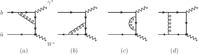
Figure 3: Diagrammatical representation of the NLO correction to the QCD correlation function $T_{\nu\mu}(p_{B},q)$ due to the hard photon radiation from the heavy bottom-quark.

Along the same vein, we can derive the renormalized hard kernel ${\cal H}_{i}^{b}$ by extracting the perturbative contributions from the one-loop QCD diagrams displayed in Figure 3

$${\cal H}_{V}^{b} = \left(\frac{4}{1-r_{3}}+1\right)\,\left({3\over 4}\ln\frac{\mu^{2}}{m^{2}_{b}}+1\right)+\left[\frac{r_{2}}{r^{2}_{1}-4\,r_{2}}\,\left(4+8\,r_{3}+r_{2}-r_{1}\,r_{2}\right)+2\,r_{2}+1\right]\,{\cal C}_{0,\,b}$$ (85)

$$+\frac{\ln(1-r_{3})}{2\,r_{3}}\,\left\{\frac{r_{2}}{r^{2}_{1}-4\,r_{2}}\,\left[-2\,(7+2\,r^{2}_{2}+5\,r_{3})+r_{1}\,(8+r_{2}+10\,r_{3})\right]+3\,r_{1}-2\right\}\,$$

$$-\frac{r_{b}\,\left(8+4\,r_{3}-r_{1}\right)}{2\,(r^{2}_{1}-4\,r_{2})}\,\,\ln\frac{2-r_{2}+r_{b}}{2}+1\,,$$

$${\cal\hat{H}}_{A}^{b} = -{\cal H}_{V}^{b}+\frac{4}{r_{1}}\,\left({3\over 4}\,\ln\frac{\mu^{2}}{m^{2}_{b}}+1\right)+\left[\frac{r_{2}}{r^{2}_{1}-4\,r_{2}}\,(8+8\,r_{3}-r_{1}\,r_{2})+\frac{r_{2}}{r_{1}}\,(8+r_{2})-4\right]\,{{\cal C}_{0,\,b}\over 2}$$ (86)

$$+\frac{\ln(1-r_{3})}{2\,r_{3}}\,\left\{\frac{r_{2}}{r^{2}_{1}-4r_{2}}\,[3\,r_{2}\,(r_{1}-2)-2\,r_{3}\,(8+r_{2})]-\frac{r_{2}\,(r_{2}+8)}{r_{1}}+2\,(2-r_{2})\right\}\,$$

$$-\frac{r_{b}\,(3+r_{3})}{r^{2}_{1}-4\,r_{2}}\,\ln\frac{2-r_{2}+r_{b}}{2}+\frac{r_{1}-r_{2}}{r_{1}}\,,$$

$${\cal\hat{H}}_{1}^{b} = \frac{4}{1-r_{3}}\,\left[\frac{r_{2}\,(r_{2}-2\,r_{1})}{r^{2}_{1}-4\,r_{2}}+1\right]\,\left({3\over 4}\,\ln\frac{\mu^{2}}{m^{2}_{b}}+1\right)+\frac{4\,r_{2}\,(r_{1}-2)}{r_{1}^{2}-4\,r_{2}}\,\left[\frac{r_{2}\,(r_{1}-r_{3}-3)}{r_{1}^{2}-4\,r_{2}}-2\right]\,{\cal C}_{0,\,b}$$

$$-\frac{2\,r_{2}}{r_{3}}\,\left\{\frac{4\,r_{2}}{(r_{1}^{2}-4\,r_{2})^{2}}\,\left[(2-r_{1})^{2}+r_{3}\,(r_{3}-2\,r_{1})\right]+\frac{5-4\,r_{1}+r_{3}\,(2+r_{3})}{r_{1}^{2}-4\,r_{2}}\right\}\,\ln(1-r_{3})$$

$$+\frac{2\,r_{b}}{r_{1}^{2}-4\,r_{2}}\,\left[\frac{2\,r_{2}\,(r_{1}-2\,r_{3}-2)}{r_{1}^{2}-4\,r_{2}}-r_{3}-5\right]\,\ln\frac{2-r_{2}+r_{b}}{2}+\frac{2\,r_{2}}{1-r_{3}}\,\frac{r_{1}\,(1+r_{3})-2\,r_{2}}{r_{1}^{2}-4\,r_{2}}\,,$$

$${\cal\hat{H}}_{2}^{b} = \left(-{r_{1}^{2}\over 4\,r_{2}}\right)\,{\cal\hat{H}}_{3}^{b}+\frac{r_{3}-1}{r_{2}}\,\left({3\over 4}\,\ln\frac{\mu^{2}}{m^{2}_{b}}+1\right)\,,$$ (88)

$${\cal\hat{H}}_{3}^{b} = \left(-{4\,r_{2}\over r_{1}^{2}}\right)\,{\cal\hat{H}}_{1}^{b}+{4\,(r_{3}-5)\over r_{1}^{2}}\,\left({3\over 4}\,\ln\frac{\mu^{2}}{m^{2}_{b}}+1\right)-{8\,r_{2}\over r_{1}^{2}}\,\frac{(3-2\,r_{2}+r_{3})\,(1-r_{3})}{r_{1}^{2}-4r_{2}}\,{\cal C}_{0,\,b}$$ (89)

$$+{4\,r_{2}\over r_{1}^{2}}\,\left[\frac{1-r_{3}}{r_{3}}\,\frac{2\,(1+3\,r_{3})-r_{1}\,(1-r_{3})}{r_{1}^{2}-4r_{2}}\right]\,\ln(1-r_{3})$$

$$-\frac{4\,r_{b}}{r_{1}^{2}}\,{8\,r_{2}+r_{1}\,(r_{3}-5)\over r_{1}^{2}-4r_{2}}\,\ln\frac{2-r_{2}+r_{b}}{2}-{4\,r_{2}\over r_{1}^{2}}\,,$$

$${\cal\hat{H}}_{4}^{b} = \left(-{r_{1}^{2}\over 4\,r_{2}}\right)\,{\cal\hat{H}}_{1}^{b}\,,$$ (90)

where for brevity we have introduced the convention

$${\cal C}_{0,\,b} = \frac{1}{\sqrt{\lambda}}\,\bigg{\{}\text{Li}_{2}\left(\frac{\xi_{1}-r_{2}\,\sqrt{\lambda}}{\xi_{1}-r_{b}\,\sqrt{\lambda}}\right)+\text{Li}_{2}\left(\frac{\xi_{1}-r_{2}\,\sqrt{\lambda}}{\xi_{1}+r_{b}\,\sqrt{\lambda}}\right)-\text{Li}_{2}\left(\frac{\xi_{1}+r_{2}\,\sqrt{\lambda}}{\xi_{1}-r_{b}\,\sqrt{\lambda}}\right)$$ (91)

$$-\,\text{Li}_{2}\left(\frac{\xi_{1}+r_{2}\,\sqrt{\lambda}}{\xi_{1}+r_{b}\,\sqrt{\lambda}}\right)-\,\text{Li}_{2}\left(\frac{\xi_{2}}{(r_{3}-1)(\xi_{3}-\sqrt{\lambda})}\right)-\,\text{Li}_{2}\left(\frac{\xi_{2}}{(r_{3}-1)(\xi_{3}+\sqrt{\lambda})}\right)$$

$$+\,\text{Li}_{2}\left(\frac{\xi_{3}-\sqrt{\lambda}}{\xi_{3}+\sqrt{\lambda}}\right)+2\,\text{Li}_{2}\left(1+\frac{\sqrt{\lambda}}{r_{3}-1}\right)-\frac{\pi^{2}}{6}\bigg{\}}\,,$$

with

$$\xi_{1} = r_{2}\,(r_{2}-r_{3}-3)\,,\qquad\xi_{2}=(r_{3}-1)\,(2-r_{1})+(1+r_{3})\,\sqrt{\lambda}\,,$$

$$\xi_{3} = 2-r_{1}\,,\qquad\hskip 45.52458ptr_{b}=\sqrt{r_{2}\,(r_{2}-4)-i\,0}\,.$$ (92)

Employing the RG evolution equations of the effective decay constant $\tilde{f}_{B}(\mu)$ as well as the bottom-quark mass $m_{b}$

$${d\tilde{f}_{B}(\mu)\over d\ln\mu} = \gamma_{\rm hl}(\alpha_{s})\,\tilde{f}_{B}(\mu)=\left[\sum_{k=0}^{\infty}\,\gamma_{k,\,\rm hl}\,\left({\alpha_{s}(\mu)\over 4\,\pi}\right)^{k+1}\right]\,\tilde{f}_{B}(\mu)\,,$$

$${d\,\overline{m}_{b}(\mu)\over d\ln\mu} = \gamma_{m}(\alpha_{s})\,\overline{m}_{b}(\mu)=\left[\sum_{k=0}^{\infty}\,\gamma_{k,\,m}\,\left({\alpha_{s}(\mu)\over 4\,\pi}\right)^{k+1}\right]\,\overline{m}_{b}(\mu)\,,$$ (93)

with the first two series coefficients given by [57, 58]

$$\gamma_{0,\,\rm hl}=3\,C_{F}\,,\qquad\gamma_{1,\,\rm hl}=C_{F}\,\left[\frac{127}{6}+\frac{14\,\pi^{2}}{9}-\frac{5}{3}\,n_{f}\right]\,,$$ (94)

and [59, 60]

$$\gamma_{0,\,m}=6\,C_{F}\,,\qquad\gamma_{1,\,m}=C_{F}\left[3\,C_{F}+{97\over 3}\,C_{A}-{20\over 3}\,n_{f}\right]\,,$$ (95)

it is then straightforward to demonstrate the factorization-scale independence of the resulting expressions for the exclusive $B_{u}^{-}\to\gamma^{\ast}\,\ell\,\bar{\nu}_{\ell}$ form factors

$${d{\cal F}_{i}^{\rm NLO}\over d\ln\mu}={\cal O}(\alpha_{s}^{2})\,,\qquad({\cal F}_{i}=F_{V},\,\hat{F}_{A},\,\hat{F}_{1,...,4})\,.$$ (96)

In analogy to the SCET factorization for the radiative leptonic $B$-meson form factors with a hard-collinear photon, the HQET decay constant $\tilde{f}_{B}(\mu)$ will be converted to the QCD decay constant $f_{B}$ by means of the matching relation (30). Subsequently, the enhanced logarithms of order $\ln\left(m_{b}/\Lambda_{\rm QCD}\right)$ entering the hard function $K^{-1}(\mu)$ will be summed at the NLL accuracy according to the second identity in (34). Importantly, the resulting NLO expressions (76) for the four-body leptonic $B$-meson form factors are observed to comply with the Ward-Takahashi constraints (16) at the accuracy of ${\cal O}(\alpha_{s})$, thus providing a valuable check of our computation.

5 Numerical results

We are now ready to explore the phenomenological implications of the obtained factorization formulae for the exclusive $B_{u}^{-}\to\gamma^{\ast}\,W^{\ast}$ form factors by applying a variety of effective field theory approaches, with an emphasis on the systematic computations of the angular observables for the four-body decay process $B_{u}^{-}\to\gamma^{\ast}(\to\ell^{\prime}\,\bar{\ell}^{\prime})\,W^{\ast}(\to\ell\,\bar{\nu}_{\ell})$ of experimental importance. To achieve this goal, we will proceed by specifying the different types of theory inputs (the electroweak parameters, the bottom-quark mass, both the leading-twist and higher-twist $B$-meson distribution amplitudes in HQET, and so on) entering the factorized expressions of the $B$-meson transition form factors emerged in the general decomposition of the corresponding decay amplitude (10).

5.1 Theory inputs

In analogy to QCD factorization for the radiative $B_{u}^{-}\to\gamma\,\ell\,\bar{\nu}_{\ell}$ decay [56], the twist-two $B$-meson distribution amplitude in HQET $\phi_{B}^{+}(\omega,\mu)$ apparently serves as the fundamental non-perturbative ingredient appearing in the SCET factorization formulae of the exclusive $B_{u}^{-}\to\gamma^{\ast}\,\ell\,\bar{\nu}_{\ell}$ form factors with a hard-collinear (off-shell) photon. Following [8], we will adopt the improved three-parameter ansatz for $\phi_{B}^{+}(\omega,\mu_{0})$ with an attractive analytical behaviour under the RG evolution at the one-loop accuracy

$$\phi_{B}^{+}(\omega,\mu_{0})={\Gamma(\beta)\over\Gamma(\alpha)}\,U\left(\beta-\alpha,3-\alpha,{\omega\over\omega_{0}}\right)\,{\omega\over\omega_{0}^{2}}\,\,{\rm exp}\left(-{\omega\over\omega_{0}}\right)\,,$$ (97)

where $U(a,b,z)$ stands for the confluent hypergeometric function of the second kind possessing an integral representation for ${\rm Re}\,[a]>0$ and ${\rm Re}\,[z]>0$

$$U(a,b,z)={1\over\Gamma(a)}\,\int_{0}^{\infty}dt\,e^{-z\,t}\,t^{a-1}\,(t+1)^{b-a-1}\,.$$ (98)

In the numerical evaluation, we will adjust the shape parameters $\omega_{0}$, $\alpha$ and $\beta$ to cover the allowed ranges for the inverse logarithmic moments of the leading-twist HQET distribution amplitude displayed in Table 1 by applying the following identities [12]

$$\lambda_{B_{u}}(\mu_{0}) = \left({\alpha-1\over\beta-1}\right)\,\omega_{0}\,,\qquad\widehat{\sigma}_{B_{u}}^{(1)}(\mu_{0})=\psi(\beta-1)-\psi(\alpha-1)+\ln\left({\alpha-1\over\beta-1}\right)\,,$$

$$\widehat{\sigma}_{B_{u}}^{(2)}(\mu_{0}) = \left[\widehat{\sigma}_{B_{u}}^{(1)}(\mu_{0})\right]^{2}+\psi^{(1)}(\alpha-1)-\psi^{(1)}(\beta-1)+{\pi^{2}\over 6}\,,$$ (99)

where the explicit definitions of $\lambda_{B_{u}}$, $\widehat{\sigma}_{B_{u}}^{(1)}$ and $\widehat{\sigma}_{B_{u}}^{(2)}$ read [8]

$$\lambda_{B_{u}}^{-1}(\mu) = \int_{0}^{\infty}\,d\omega\,\,{\phi_{B}^{+}(\omega,\mu)\over\omega}\,,$$

$$\widehat{\sigma}_{B_{u}}^{(n)}(\mu) = \lambda_{B_{u}}(\mu)\,\int_{0}^{\infty}\,{d\omega\over\omega}\,\left[\ln\left({\lambda_{B_{u}}(\mu)\over\omega}\right)-\gamma_{E}\right]^{n}\,\phi_{B}^{+}(\omega,\mu)\,.$$ (100)

Substituting (98) into the constructed solution (34) to the Lange-Neubert evolution equation [34] results in (see [8] for the RG evolution function in coordinate space)

$$\phi_{B}^{+}(\omega,\mu)$$

$$={\rm exp}\bigg{\{}-{\Gamma_{\rm cusp}^{(0)}\over 4\,\beta_{0}^{2}}\,\bigg{[}{4\pi\over\alpha_{s}(\mu_{0})}\,\left(\ln{\alpha_{s}(\mu)\over\alpha_{s}(\mu_{0})}-1+{\alpha_{s}(\mu_{0})\over\alpha_{s}(\mu)}\right)-{\beta_{1}\over 2\,\beta_{0}}\,\ln^{2}{\alpha_{s}(\mu)\over\alpha_{s}(\mu_{0})}+\left({\Gamma_{\rm cusp}^{(1)}\over\Gamma_{\rm cusp}^{(0)}}-{\beta_{1}\over\beta_{0}}\right)$$

$$\hskip 42.67912pt\times\left({\alpha_{s}(\mu)\over\alpha_{s}(\mu_{0})}-1-\ln{\alpha_{s}(\mu)\over\alpha_{s}(\mu_{0})}\right)\bigg{]}\bigg{\}}\,\,\left({\alpha_{s}(\mu)\over\alpha_{s}(\mu_{0})}\right)^{\gamma_{\eta}^{(0)}/(2\,\beta_{0})}\,\left({1\over\omega_{0}}\right)\,\left({\mu_{0}\,e^{2\,\gamma_{E}}\over\omega_{0}}\right)^{\kappa_{s}}$$

$$\hskip 14.22636pt\times\,\bigg{\{}{\omega\over\omega_{0}}\,\,\frac{\Gamma(\beta)\,\Gamma(2+\kappa_{s})\,\Gamma(\alpha-\kappa_{s}-2)}{\Gamma(\alpha)\,\Gamma(\beta-\kappa_{s}-2)}\,\,{}_{2}F_{2}\left(\kappa_{s}+2,\kappa_{s}+3-\beta;2,\kappa_{s}+3-\alpha,-{\omega\over\omega_{0}}\right)$$

$$\hskip 22.76228pt+\left({\omega\over\omega_{0}}\right)^{\alpha-\kappa_{s}-1}\,\,\frac{\Gamma(\beta)\,\Gamma(2+\kappa_{s}-\alpha)}{\Gamma(\beta-\alpha)\,\Gamma(\alpha-\kappa_{s})}\,\,{}_{2}F_{2}\left(\alpha,\alpha-\beta+1;\alpha-\kappa_{s}-1,\alpha-\kappa_{s},-{\omega\over\omega_{0}}\right)\bigg{\}}\,,\hskip 28.45274pt$$ (101)

where the expansion coefficient $\kappa_{s}$ is explicitly defined by

$$\kappa_{s}={\Gamma_{\rm cusp}^{(0)}\over 2\,\beta_{0}}\,\ln{\alpha_{s}(\mu)\over\alpha_{s}(\mu_{0})}\,.$$ (102)

In comparison with QCD factorization for the exclusive non-hadronic $B$-meson decays $B_{u}^{-}\to\gamma\,\ell\,\bar{\nu}_{\ell}$ [5, 6, 7, 8] and $\bar{B}_{d,\,s}\to\gamma\gamma$ [63, 64, 12] in the heavy quark limit, the LP contributions to the generalized $B_{u}^{-}\to\gamma^{\ast}\,W^{\ast}$ form factors presented in (29) are more sensitive to the precise shape of the twist-two distribute amplitude $\phi_{B}^{+}(\omega,\mu_{0})$ rather than determined by the inverse moment $\lambda_{B}(\mu_{0})$ completely at the one-loop accuracy. Consequently, the four-body leptonic $B$-meson decays under discussion are expected to provide us with abundant opportunities for probing the partonic landscape of the heavy-quark hadron system delicately.

Parameter	Value	Ref.	Parameter	Value	Ref.
$G_{F}$	$1.166379\times 10^{-5}\,\,{\rm GeV}^{-2}$	[61]	$|V_{ub}|$	$(3.70\pm 0.10\pm 0.12)\times 10^{-3}$	[61]
$\alpha_{s}^{(5)}(m_{Z})$	$0.1188\pm 0.0017$	[61]	$\alpha_{\rm em}^{(5)}(m_{Z})^{-1}$	$127.952\pm 0.009$	[61]
$m_{e}$	$0.511$ MeV	[61]	$m_{\mu}$	$105.658$ MeV	[61]
$\overline{m}_{b}(\overline{m}_{b})$	$4.198\pm 0.012$ GeV	[61]	$m_{b}^{\rm PS}(2\,{\rm GeV})$	$4.532^{+0.013}_{-0.039}$ GeV	[62]
$m_{B_{u}}$	$5279.34\pm 0.12$ MeV	[61]	$\tau_{B_{u}}$	$(1.638\pm 0.004)$ ps	[61]
$f_{B_{u}}|_{N_{f}=2+1+1}$	$190.0\pm 1.3$ MeV	[24]
$\lambda_{B_{u}}(\mu_{0})$	$(350\pm 150)$ MeV	[11]		$\{0.7,\,6.0\}$
$\lambda_{E}^{2}(\mu_{0})/\lambda_{H}^{2}(\mu_{0})$	$0.50\pm 0.10$	[8]	$\{\widehat{\sigma}_{B_{u}}^{(1)}(\mu_{0}),\,\widehat{\sigma}_{B_{u}}^{(2)}(\mu_{0})\}$	$\{0.0,\,\pi^{2}/6\}$	[11]
$2\,\lambda_{E}^{2}(\mu_{0})+\lambda_{H}^{2}(\mu_{0})$	$(0.25\pm 0.15)\,{\rm GeV^{2}}$	[8]		$\{-0.7,\,-6.0\}$

Table 1: The numerical values of the various input parameters employed in the theory predictions for the four-body leptonic $B$-meson decays.

Moreover, the two-particle and three-particle higher-twist $B$-meson distribution amplitudes in HQET are evidently indispensable for evaluating the LP contributions to the two radiative form factors $\hat{F}_{2(4),\,\rm LP}$ collected in (27) and (29) as well as the subleading power corrections calculable with the perturbative factorization technique displayed in (51), (53), (62) and (65). Following [8, 12] we will adopt the concrete phenomenological models fulfilling the classical equations of motion and the corresponding asymptotic behaviour at small quark and gluon momenta from the conformal spin analysis [65] (see [43, 7] for the two sample choices of the higher-twist distribution amplitudes at the twist-six accuracy)

$$\phi_{B}^{-}(\omega,\mu_{0})=\phi_{B}^{-,\,\rm WW}(\omega,\mu_{0})+\phi_{B}^{-,\,\rm tw3}(\omega,\mu_{0})$$

$$=\left[\int_{\omega}^{\infty}d\rho\,f(\rho)\right]+{1\over 6}\,\varkappa(\mu_{0})\,\left[\lambda_{E}^{2}(\mu_{0})-\lambda_{H}^{2}(\mu_{0})\right]\,\left[\omega^{2}\,f^{\prime}(\omega)+4\,\omega\,f(\omega)-2\,\int_{\omega}^{\infty}d\rho\,f(\rho)\right],$$

$$\phi_{3}(\omega_{1},\omega_{2},\mu_{0})=-{1\over 2}\,\varkappa(\mu_{0})\,\left[\lambda_{E}^{2}(\mu_{0})-\lambda_{H}^{2}(\mu_{0})\right]\,\omega_{1}\,\omega_{2}^{2}\,f^{\prime}(\omega_{1}+\omega_{2})\,,$$

$$\phi_{4}(\omega_{1},\omega_{2},\mu_{0})={1\over 2}\,\varkappa(\mu_{0})\,\left[\lambda_{E}^{2}(\mu_{0})+\lambda_{H}^{2}(\mu_{0})\right]\,\omega_{2}^{2}\,f(\omega_{1}+\omega_{2})\,,$$

$$\psi_{4}(\omega_{1},\omega_{2},\mu_{0})=\varkappa(\mu_{0})\,\lambda_{E}^{2}(\mu_{0})\,\omega_{1}\,\omega_{2}\,f(\omega_{1}+\omega_{2})\,,$$

$$\tilde{\psi}_{4}(\omega_{1},\omega_{2},\mu_{0})=\varkappa(\mu_{0})\,\lambda_{H}^{2}(\mu_{0})\,\omega_{1}\,\omega_{2}\,f(\omega_{1}+\omega_{2})\,,$$

$$\psi_{5}(\omega_{1},\omega_{2},\mu_{0})=\varkappa(\mu_{0})\,\lambda_{E}^{2}(\mu_{0})\,\omega_{2}\,\int_{\omega_{1}+\omega_{2}}^{\infty}d\eta\,f(\eta),$$

$$\tilde{\psi}_{5}(\omega_{1},\omega_{2},\mu_{0})=\varkappa(\mu_{0})\,\lambda_{H}^{2}(\mu_{0})\,\omega_{2}\,\int_{\omega_{1}+\omega_{2}}^{\infty}d\eta\,f(\eta),$$

$$\phi_{6}(\omega_{1},\omega_{2},\mu_{0})=\varkappa(\mu_{0})\,\left[\lambda_{E}^{2}(\mu_{0})-\lambda_{H}^{2}(\mu_{0})\right]\,\int_{\omega_{1}+\omega_{2}}^{\infty}d\eta_{1}\,\int_{\eta_{1}}^{\infty}\,d\eta_{2}\,f(\eta_{2}),$$ (103)

which further enable us to determine two-particle twist-four and twist-five distribution amplitudes $g_{B}^{\pm}(\omega,\mu_{0})$ by virtue of the obtained identities (58) and (59). The non-perturbative profile function $f(\omega)$ and the normalization constant $\varkappa(\mu_{0})$ are given by

$$f(\omega) = {\Gamma(\beta)\over\Gamma(\alpha)}\,U\left(\beta-\alpha,3-\alpha,{\omega\over\omega_{0}}\right)\,{1\over\omega_{0}^{2}}\,\,{\rm exp}\left(-{\omega\over\omega_{0}}\right)\,,$$

$$\varkappa^{-1}(\mu_{0}) = {1\over 2}\,\int_{0}^{\infty}d\omega\,\omega^{3}\,f(\omega)=\bar{\Lambda}^{2}+{1\over 6}\,\left[2\,\lambda_{E}^{2}(\mu_{0})+\lambda_{H}^{2}(\mu_{0})\right]\,.$$ (104)

The appearing HQET parameters $\lambda_{E}^{2}$ and $\lambda_{H}^{2}$ can be defined in terms of the local effective matrix element of the dimension-five quark-gluon operator [43, 45]

$$\langle 0|\bar{q}(0)\,g_{s}\,G_{\mu\nu}\,\Gamma\,h_{v}(0)|\bar{B}_{q}(v)\rangle$$

$$=-{\tilde{f}_{B_{q}}\,m_{B_{q}}\over 6}\,{\rm Tr}\left\{\gamma_{5}\,\Gamma\,\,\left({1+\not{v}\over 2}\right)\,\left[\lambda_{H}^{2}\,\left(i\,\sigma_{\mu\nu}\right)+(\lambda_{H}^{2}-\lambda_{E}^{2})\,\left(v_{\mu}\,\gamma_{\nu}-v_{\nu}\,\gamma_{\mu}\right)\right]\right\}\,.$$ (105)

The RG evolution equations for $\lambda_{E}^{2}$ and $\lambda_{H}^{2}$ at the one-loop accuracy read [66, 67]

$${d\over d\ln\mu}\,\left(\begin{array}[]{c}\lambda_{E}^{2}(\mu)\\ \lambda_{H}^{2}(\mu)\\ \end{array}\right)+\gamma_{\rm EH}\,\left(\begin{array}[]{c}\lambda_{E}^{2}(\mu)\\ \lambda_{H}^{2}(\mu)\\ \end{array}\right)=0\,,$$ (110)

where the anomalous dimension matrix $\gamma_{\rm EH}$ takes the form

$$\gamma_{\rm EH}={\alpha_{s}(\mu)\over 4\,\pi}\left(\begin{array}[]{cc}{8\over 3}\,C_{F}+{3\over 2}\,N_{c}&\,\,{4\over 3}\,C_{F}-{3\over 2}\,N_{c}\\ {4\over 3}\,C_{F}-{3\over 2}\,N_{c}&\,\,{8\over 3}\,C_{F}+{5\over 2}\,N_{c}\\ \end{array}\right)+{\cal O}(\alpha_{s}^{2})\,.$$ (113)

The manifest solution to (110) can be readily constructed by diagonalizing the achieved $2\times 2$ mixing matrix $\gamma_{\rm EH}$ [66, 16]. The available predictions of these two HQET quantities from the method of two-point QCD sum rules can be summarized as follows

$$\left\{\lambda_{E}^{2}(\mu_{0}),\,\,\lambda_{H}^{2}(\mu_{0})\right\}=\left\{\begin{array}[]{l}\left\{(0.11\pm 0.06)\,{\rm GeV^{2}},\,\,(0.18\pm 0.07)\,{\rm GeV^{2}}\right\}\,,\qquad\hskip 42.67912pt\text{\cite[cite]{[\@@bibref{Number}{Grozin:1996pq}{}{}]}}\vspace{0.5 cm}\\ \left\{(0.03\pm 0.02)\,{\rm GeV^{2}},\,\,(0.06\pm 0.03)\,{\rm GeV^{2}}\right\}\,,\qquad\hskip 42.67912pt\text{\cite[cite]{[\@@bibref{Number}{Nishikawa:2011qk}{}{}]}}\vspace{0.5 cm}\\ \left\{(0.01\pm 0.01)\,{\rm GeV^{2}},\,\,(0.15\pm 0.05)\,{\rm GeV^{2}}\right\}\,.\qquad\hskip 42.67912pt\text{\cite[cite]{[\@@bibref{Number}{Rahimi:2020zzo}{}{}]}}\end{array}\hskip 22.76228pt\right.$$ (117)

Apparently, the yielding results for the chromo-electric and chromo-magnetic matrix elements deviate from each other significantly despite the implementations of the same calculational framework. The dominating discrepancies for the numerical values displayed in [68] and [67] can be attributed to the sizeable QCD radiative correction to the dimension-five quark-gluon condensate and the yet higher-power contribution from the dimension-six vacuum condensate at tree level, which have been included in the updated computation [67] with a further improvement on the (partial)-NLL resummation of the emerged large logarithms appearing in the HQET sum rules. Instead of constructing the desired sum rules from the appropriate correlation functions with one two-body and one three-body local current, the authors of [69] suggested to employ the diagonal Green functions for the sake of obtaining the alternative sum rules for $\lambda_{E}^{2}$ and $\lambda_{H}^{2}$, with the expectation that the parton-hadron duality approximation becomes more reliable due to the positive definite property obviously. Introducing the higher dimensional correlation functions, however, turns out to worsen the OPE convergence in contrast to the previously adopted non-diagonal ones, as already observed in [69]. In view of an absence of the satisfactory evaluation for these two non-perturbative parameters, we will follow closely the strategy of [8, 12] such that the numerical intervals of the combinations $\lambda_{E}^{2}/\lambda_{H}^{2}$ and $2\,\lambda_{E}^{2}+\lambda_{H}^{2}$ collected in Table 1 accommodate the obtained results from the two-point sum rules [68, 67] and particularly lie within the upper bounds for $\lambda_{E}^{2}$ and $\lambda_{H}^{2}$ derived from the diagonal correlation functions [69]. In addition, the HQET parameter $\bar{\Lambda}$ entering the soft-collinear factorization formulae (51) and (62) can be identified as the “effective mass” of the heavy-meson state [45, 55]: $\bar{\Lambda}=m_{B_{u}}-m_{b}+{\cal O}(\Lambda_{\rm QCD}^{2}/m_{b})$, where we will take $m_{b}=(4.8\pm 0.1)\,{\rm GeV}$ numerically following the standard arguments presented in [8, 12].

Now we turn to discuss the practical implementations the interesting SM parameters appeared in the exclusive $B_{u}^{-}\to\gamma^{\ast}\,\ell\,\bar{\nu}_{\ell}$ decay form factors. The strong coupling constant $\alpha_{s}(\mu)$ in the $\overline{\rm MS}$ scheme will be computed from the initial condition $\alpha_{s}^{(5)}(m_{Z})$ summarized in Table 1 with the associated three-loop RG evolution equation, by further adopting the quark-flavour threshold scales $\mu_{4}=4.8\,{\rm GeV}$ and $\mu_{3}=1.2\,{\rm GeV}$ for crossing $n_{f}=4$ and $n_{f}=3$, respectively. Furthermore, the bottom-quark mass entering the perturbative hard matching functions (21) is generally interpreted as the pole mass due to the on-shell kinematics [10, 30, 11, 12]. However, the bottom-quark pole mass suffers from an intrinsic ambiguity of order $\Lambda_{\rm QCD}$ known as the infrared renormalon (see [70] for an excellent review). We will therefore employ the potential-subtracted (PS) renormalization scheme for the bottom-quark mass [71] and then convert the obtained expressions of the hard functions from the pole scheme to the PS scheme for the mass parameter accordingly (see [72] for an overview of the leading renormalon-free and short-distance mass definitions for nearly on-shell heavy quarks). Another important hadronic quantity governing the factorized result for the four-body rare $B$-meson decay amplitude in the entire kinematic region is the leptonic decay constant of the charged bottom-meson $f_{B_{u}}$, whose interval collected in Table 1 is borrowed from the lattice-QCD computation with the number of dynamical quark flavours $N_{f}=2+1+1$ in the isospin symmetry limit [24] (see [73] for the further discussion on the strong-isospin violating effect and [74, 75, 76] on the technical strategies to address the more complicated electromagnetic correction).

Apart from the theory input parameters so far discussed, we still need to specify the hard scales $\mu_{h1}$ and $\mu_{h2}$ entering the resummation improved hard functions $C_{V}^{({\rm A0}),\,1}$ and $K^{-1}$ presented in (34), which will be varied in the interval $\mu_{h1}=\mu_{h2}\in[m_{b}/2,\,\,2\,m_{b}]$ around the default value $m_{b}$. Additionally, the factorization scale $\mu$ in the SCET expressions (3.1), (26), (27), (28), (29) will be taken as $\mu\in[1.0,2.0]\,{\rm GeV}$ with the central value $1.5\,{\rm GeV}$. By contrast, the allowed interval of the factorization scale $\mu$ appearing in the HQET expression (76) will naturally read $[m_{b}/2,\,\,2\,m_{b}]$ in that the typical short-distance fluctuation mode carries out the four-momentum $p_{\mu}\sim{\cal O}(m_{b})$.

5.2 Theory predictions for the $B_{u}^{-}\to\gamma^{\ast}\,\ell\,\bar{\nu}_{\ell}$ form factors

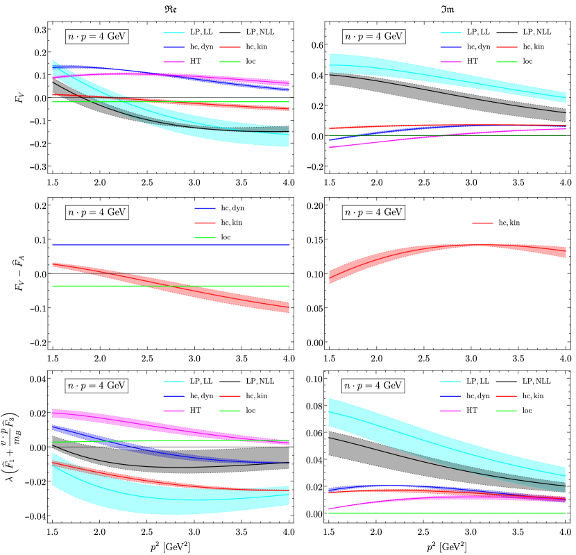
Figure 4: Breakdown of the distinct QCD mechanisms contributing to the transverse and longitudinal transition form factors involved in the four-body leptonic decay amplitude (10) in the kinematical region $p^{2}\in[1.5,\,4.0]\,{\rm GeV^{2}}$, with the theory uncertainties due to the variations of the hard and hard-collinear scales indicated by the individual bands. The representative value of the large component $n\cdot p$ for the virtual photon momentum is taken as $4.0\,{\rm GeV}$.

We proceed to investigate the numerical impacts of the newly derived QCD radiative corrections and the subleading power contributions to the three transition form factors appearing in the four-body leptonic decay amplitude (10) in the entire kinematic region. To facilitate detailed explorations of the dynamical patterns dictating the exclusive $B_{u}^{-}\to\gamma^{\ast}\,\ell\,\bar{\nu}_{\ell}$ form factors with a hard-collinear photon, we first display the obtained leading-power contributions at the leading-logarithmic (LL) and NLL accuracy, the power suppressed corrections from expanding the hard-collinear quark propagator in the small parameter $\Lambda_{\rm QCD}/m_{b}$ beyond the LP approximation, the higher-twist contributions from the two-particle and three-particle $B$-meson distribution amplitudes, the “kinematic” power corrections presented in (65), and the local NLP contributions due to the off-shell photon radiation from the heavy bottom quark at $1.5\,{\rm GeV^{2}}\leq p^{2}\leq 4.0\,{\rm GeV^{2}}$ in Figure 4, where the perturbative uncertainties from varying the hard scales $\mu_{h1}$ and $\mu_{h2}$ as well as the factorization scale $\mu$ are further indicated by the yielding bands. The resulting uncertainties from the NLL resummation improved predictions are evidently much less than the counterpart LL computations. In particular, the achieved LL and NLL uncertainty bands for the imaginary part of the vector form factor ${\rm Im}\,F_{V}$ turn out to be well separated in the majority of the hard-collinear $p^{2}$ regime. The peculiar behaviours of the LP contributions to the two complex-valued form factors $F_{V}$ and $\hat{F}_{1}+{v\cdot p\over m_{B}}\,\hat{F}_{3}$ can be traced back to the soft-collinear convolution integrals in the SCET factorization formulae (3.1), (26), (27), (28), (29) which are effectively controlled by the generalized inverse moments $\lambda_{B}^{\pm}(\bar{n}\cdot p,\mu)$ of the two-particle $B$-meson distribution amplitudes in HQET . Applying the exponential model of $\phi_{B}^{\pm}(\omega,\mu_{0})$ [68] as an illustrative example, the distinctive features of the two inverse moments displayed in Figure 5 are indeed observed to dictate the intricate photon-momentum dependence of the transverse and longitudinal decay form factors, respectively. Furthermore, it is plainly not unexpected to discover from Figure 4 the increasing significance of the “kinematic power corrections” to the two essential form factors $|F_{V}|$ and $\left|\lambda\,\left(\hat{F}_{1}+{v\cdot p\over m_{B}}\,\hat{F}_{3}\right)\right|$, when the off-shellness the hard-collinear photon moves towards higher values. The very prominent subleading power contributions from the hard-collinear quark propagator at tree level will consistently shift the LL predictions of $|F_{V}|$ and $\left|\lambda\,\left(\hat{F}_{1}+{v\cdot p\over m_{B}}\,\hat{F}_{3}\right)\right|$ by an amount of approximately $(20-30)\,\%$ for $1.5\,{\rm GeV}^{2}\leq p^{2}\leq\,4.0{\rm GeV}^{2}$. In addition, they constitute an important source of generating the large-recoil symmetry violation $|F_{V}-\hat{F}_{A}|$ between the vector and axial-vector form factors, which is constructed to characterize the power suppressed terms in the heavy quark expansion conveniently [5]. Our numerical studies of the subleading twist contributions to the radiative leptonic $B$-meson form factors summarized in (53) and (62) imply that the magnitudes of the yielding three-particle higher-twist corrections are at least suppressed by a factor of twenty when compared with the corresponding two-particle NLP effects in virtue of the smallness of the two normalization constants $\lambda_{E}^{2}$ and $\lambda_{H}^{2}$. Unsurprisingly, the local subleading power contributions (66) from the HQET formalism will bring about insignificant impacts on the exclusive non-hadronic $B_{u}^{-}\to\gamma^{\ast}\,W^{\ast}$ decay form factors: $(4-6)\%$ for $|F_{V}|$ and $(4-10)\%$ for $\left|\lambda\,\left(\hat{F}_{1}+{v\cdot p\over m_{B}}\,\hat{F}_{3}\right)\right|$ numerically, which are in accordance with the previous observation in the context of $B\to\gamma\,\ell\,\bar{\nu}_{\ell}$ [7].

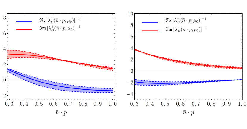
Figure 5: The photon-momentum dependence of the generalized inverse moments $\lambda_{B}^{\pm}(\bar{n}\cdot p,\mu)$ for the two-particle $B$-meson distribution amplitudes by employing the exponential model proposed in [68] for illustration purposes. The uncertainty bands arise from the variation of the non-perturbative shape parameter $\omega_{0}\in[300,400]\,{\rm MeV}$.

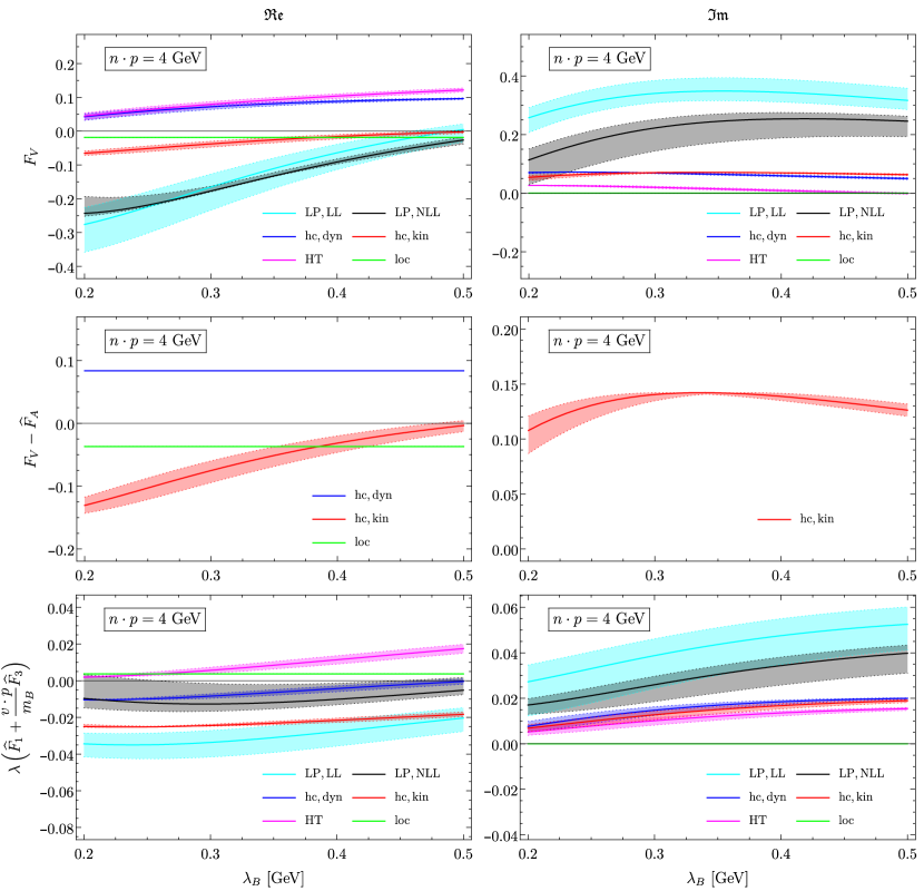
Figure 6: Theory predictions for the inverse-moment dependencies of all separate pieces contributing to the radiative $B_{u}^{-}\to\gamma^{\ast}\,W^{\ast}$ form factors in the decay amplitude (10) in the interval $\lambda_{B_{u}}\in[200,500]\,{\rm MeV}$, with the uncertainty bands from varying the hard and hard-collinear scales. The representative values of the large and small components for the virtual photon momentum are taken as $4.0\,{\rm GeV}$ and $0.75\,{\rm GeV}$.

We further present in Figure 6 the obtained theory predictions for the individual pieces contributing to the three form factors of our interest, as the analytical functions of the inverse moment $\lambda_{B_{u}}$, by adopting the input kinematic parameters $n\cdot p=4.0\,{\rm GeV}$ and $\bar{n}\cdot p=0.75\,{\rm GeV}$. Interestingly, the LP contribution of the vector form factor $|F_{V}|$ turns out to be significantly more sensitive to $\lambda_{B_{u}}$ than that for the longitudinal form factor $\left|\lambda\,\left(\hat{F}_{1}+{v\cdot p\over m_{B}}\,\hat{F}_{3}\right)\right|$, stemming from the different asymptotic behaviours of the very $B$-meson distribution amplitudes at small quark and gluon momenta, which appear in the LP soft-collinear factorization formulae (3.1), (26), (27), (28), (29). It is further worth mentioning that the two-particle subleading twist corrections to both form factors $|F_{V}|$ and $\left|\lambda\,\left(\hat{F}_{1}+{v\cdot p\over m_{B}}\,\hat{F}_{3}\right)\right|$ develop the yet stronger $\lambda_{B_{u}}$-dependence in comparison with the counterpart lower-twist contributions from $\phi_{B}^{+}(\omega,\mu)$ and $\phi_{B}^{-}(\omega,\mu)$. Additionally, the inverse-moment dependence of the helicity form factor $|F_{V}-\hat{F}_{A}|$ originates from the “kinematic” power corrections (65) entirely, keeping in mind that the NLP dynamical contributions displayed in (51) merely generate the “local” large-recoil symmetry breaking effects independent of the higher-twist $B$-meson distribution amplitudes.

Figure 7: The predicted photon-momentum dependencies of the three transition form factors governing the four-body leptonic $B$-meson decay amplitude (10) with three sample choices of the dimensionless shape parameters $\widehat{\sigma}_{B_{u}}^{(1)}$ and $\widehat{\sigma}_{B_{u}}^{(2)}$, but with fixed $\lambda_{B_{u}}(\mu_{0})=350\,{\rm MeV}$, characterizing the non-perturbative behaviours of the leading-twist distribution amplitude $\phi_{B}^{+}(\omega,\mu_{0})$.

In contrast to QCD factorization for $B\to\gamma\,\ell\,\bar{\nu}_{\ell}$ with an on-shell photon, the LP contributions of the non-hadronic radiative $B_{u}^{-}\to\gamma^{\ast}\,\ell\,\bar{\nu}_{\ell}$ form factors in the heavy quark expansion cannot be determined by the inverse moment $\lambda_{B_{u}}(\mu_{0})$ completely even without taking into account the higher-order gluonic corrections. It is therefore interesting to explore the actual dependencies of the exclusive $B$-meson decay form factors on the intricate shapes of the HQET distribution amplitudes, along the lines of [33, 13, 77, 50]. To this end, we show in Figure 7 the achieved predictions of the exclusive $B_{u}^{-}\to\gamma^{\ast}\,W^{\ast}$ form factors with three sample choices of the model parameters $\widehat{\sigma}_{B_{u}}^{(1)}$ and $\widehat{\sigma}_{B_{u}}^{(2)}$ for fixed $\lambda_{B_{u}}(\mu_{0})=350\,{\rm MeV}$ in the kinematic domain $p^{2}\in[1.5,\,4.0]\,{\rm GeV^{2}}$. It is not surprising to observe the pronounced sensitivities of both the transverse and longitudinal form factors under discussion to the precise shapes of the $B$-meson distribution amplitudes, which are in accordance with the previous observations on the SCET sum-rule computations for heavy-to-light $B$-meson decay form factors at large recoil [15, 16]. We are then led to conclude that the four-body leptonic bottom-meson decay processes allow us to probe the partonic landscape of the heavy-hadron system diversely, in a complementary manner to the semi-leptonic and electroweak penguin decays of $B$-mesons [78, 20, 21, 79], with the aid of the upcoming sufficient experimental data.

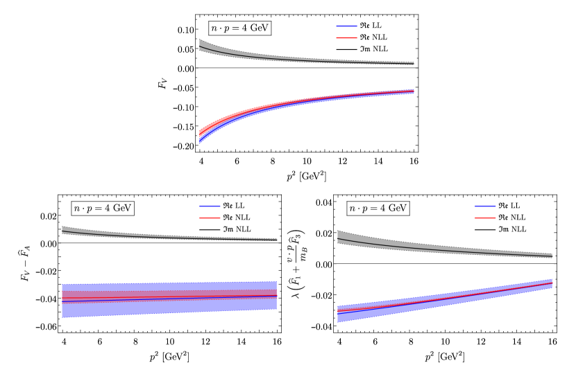
Figure 8: Theory predictions for the photon-momentum dependencies of the exclusive $B_{u}^{-}\to\gamma^{\ast}\,\ell\,\bar{\nu}_{\ell}$ form factors with an off-shell photon carrying the hard momentum $p_{\mu}\sim{\cal O}(m_{b})$ in the LP approximation. The uncertainty bands are obtained by varying the factorization scale in the allowed intervals of $\mu\in[m_{b}/2,\,\,2\,m_{b}]$.

We now turn to display the LP contributions to the radiative leptonic $B_{u}^{-}\to\gamma^{\ast}\,\ell\,\bar{\nu}_{\ell}$ form factors in the kinematic regime $p^{2}\in[4.0,\,16.0]\,{\rm GeV^{2}}$ at the LL and NLL accuracy in Figure 8, where the residual perturbative uncertainties from varying the factorization scale are further represented by the individual bands. Unlike the factorized expressions for the exclusive $B_{u}^{-}\to\gamma^{\ast}\,\ell\,\bar{\nu}_{\ell}$ form factors with a hard-collinear photon, the counterpart contributions of these form factors in the hard $p^{2}$ region are apparently the real-valued functions at ${\cal O}(\alpha_{s}^{0})$. The emerged strong phases for $F_{V(A)}$ and $\left(\hat{F}_{1}+{v\cdot p\over m_{B}}\,\hat{F}_{3}\right)$ at the NLL accuracy are generated perturbatively by the four one-loop diagrams shown in Figure 2, which can be understood from the final-state rescattering mechanism $B_{u}^{-}\to X_{u\,\bar{u}}\,\ell\,\bar{\nu}_{\ell}\to\ell^{\prime}\,\bar{\ell}^{\prime}\,\ell\,\bar{\nu}_{\ell}$ at hadronic level with $X_{u\,\bar{u}}$ standing for the appropriate neutral light-hadron states. Moreover, the higher-order QCD corrections to both the transverse and longitudinal form factors at ${\cal O}(\alpha_{s})$ will give rise to the very minor impacts on the corresponding tree-level predictions at $4.0\,{\rm GeV^{2}}\leq p^{2}\leq 16.0\,{\rm GeV^{2}}$ (numerically less than $10\%$ in magnitudes). In particular, the NLL resummation improved computations are highly beneficial for pining down the theory uncertainties of the LL QCD predictions effectively.

5.3 Differential decay distribution for $B_{u}^{-}\to\ell^{\prime}\,\bar{\ell}^{\prime}\,\ell\,\bar{\nu}_{\ell}$

Having at our disposal the theory predictions for the exclusive radiative $B_{u}^{-}\to\gamma^{\ast}\,\ell\,\bar{\nu}_{\ell}$ form factors, we are now in a position to address the phenomenological aspects of the four-body leptonic $B$-meson decays with an emphasis on the numerous decay observables of experimental interest. In doing so, we begin to derive the five-fold differential decay width for the process $B_{u}^{-}\to\ell^{\prime}\,\bar{\ell}^{\prime}\,\ell\,\bar{\nu}_{\ell}$ with non-identical lepton flavours in terms of the two invariant masses $p^{2}$ and $q^{2}$ as well as the three angles $\theta_{1}$, $\theta_{2}$ and $\phi$ (see Appendix A for the detailed definitions)

$$\frac{d^{5}\Gamma(B_{u}^{-}\to\ell^{\prime}\,\bar{\ell}^{\prime}\,\ell\,\bar{\nu}_{\ell})}{dp^{2}\,dq^{2}\,d\cos\theta_{1}\,d\cos\theta_{2}\,d\phi} = \frac{G_{F}^{2}\,\alpha_{\rm em}^{2}\,|V_{ub}|^{2}}{2^{12}\,\pi^{4}\,p^{4}}\,m_{B}^{3}\,\,\lambda^{1/2}(m_{B}^{2},p^{2},q^{2})\,{\cal J}(p^{2},\,q^{2},\,\theta_{1},\,\theta_{2},\,\phi)\,,$$ (118)

$$= {\cal N}(p^{2},q^{2})\,{\cal J}(p^{2},\,q^{2},\,\theta_{1},\,\theta_{2},\,\phi)\,,$$

by employing the explicit expression of the obtained decay amplitude (10) and by further summing over spins of the final-state particles. It is straightforward to decompose the angular distribution ${\cal J}$ into a set of the trigonometric functions

$${\cal J}(p^{2},\,q^{2},\,\theta_{1},\,\theta_{2},\,\phi) = J_{1}\,(1+\cos^{2}\theta_{1})\,(1+\cos^{2}\theta_{2})+J_{2}\,\sin^{2}\theta_{1}\,\sin^{2}\theta_{2}+J_{3}\,(1+\cos^{2}\theta_{1})\,\cos\theta_{2}$$ (119)

$$+\left[J_{4}\,\sin\theta_{2}+J_{5}\,\sin\,(2\,\theta_{2})\right]\,\,\sin\,(2\,\theta_{1})\,\sin\phi$$

$$+\left[J_{6}\,\sin\theta_{2}+J_{7}\,\sin\,(2\,\theta_{2})\right]\,\,\sin\,(2\,\theta_{1})\,\cos\phi$$

$$+J_{8}\,\sin^{2}\theta_{1}\,\sin^{2}\theta_{2}\,\sin\,(2\,\phi)+J_{9}\,\sin^{2}\theta_{1}\,\sin^{2}\theta_{2}\,\cos\,(2\,\phi)\,,$$

where the nine independent coefficient functions $J_{i}\equiv J_{i}(p^{2},q^{2})$ ($i=1,...,9$) can be expressed by the three radiative bottom-meson decay form factors

$$J_{1} = \frac{1}{4}\,\left[|\widetilde{F}_{A}|^{2}+|\widetilde{F}_{V}|^{2}\right]\,,$$

$$J_{2} = \frac{1}{2}\,\left[|\widetilde{\mathbb{F}}_{A}|^{2}+|\widetilde{F}_{\|}|^{2}+2\,{\rm Re}\,\left(\widetilde{\mathbb{F}}_{A}\,\widetilde{F}_{\|}^{\ast}\right)\right]\,,$$

$$J_{3} = {\rm Re}\,\left(\widetilde{F}_{A}\,\widetilde{F}_{V}^{\ast}\right)\,,$$

$$J_{4} = \frac{1}{2}\,{\rm Im}\,\left(\widetilde{F}_{A}\,\widetilde{F}_{\|}^{\ast}\right)\,,$$

$$J_{5} = \frac{1}{4}\,{\rm Im}\,\left(\widetilde{F}_{V}\,\widetilde{\mathbb{F}}_{A}^{\ast}+\widetilde{F}_{V}\,\widetilde{F}_{\|}^{\ast}\right)\,,$$

$$J_{6} = -\frac{1}{2}\,{\rm Re}\,\left(\widetilde{F}_{V}\,\widetilde{\mathbb{F}}_{A}^{\ast}+\widetilde{F}_{V}\,\widetilde{F}_{\|}^{\ast}\right)\,,$$

$$J_{7} = -\frac{1}{4}\,\left[|\widetilde{F}_{A}\,\widetilde{\mathbb{F}}_{A}|+{\rm Re}\,\left(\widetilde{F}_{A}\,\widetilde{F}_{\|}^{\ast}\right)\right]\,,$$

$$J_{8} = \frac{1}{2}\,{\rm Im}\,\left(\widetilde{F}_{A}\,\widetilde{F}_{V}^{\ast}\right)\,,$$

$$J_{9} = \frac{1}{4}\,\left[|\widetilde{F}_{A}|^{2}-|\widetilde{F}_{V}|^{2}\right]\,.$$ (120)

We have introduced the shorthand notations for the distinct combinations of the transition form factors with the appropriate kinematic functions

$$\widetilde{F}_{V} = 2\,\sqrt{\hat{p}^{2}\,\hat{q}^{2}\,\lambda(1,\hat{p}^{2},\,\hat{q}^{2})}\,F_{V}\,,\qquad\widetilde{F}_{A}=2\,\sqrt{\hat{p}^{2}\,\hat{q}^{2}}\,(1+\hat{p}^{2}-\hat{q}^{2})\,F_{A}\,,$$

$$\widetilde{\mathbb{F}}_{A} = \left[(1-\hat{q}^{2})^{2}-\hat{p}^{4}\right]\,F_{A}\,,\qquad\hskip 21.33955pt\widetilde{F}_{\|}=\lambda(1,\hat{p}^{2},\,\hat{q}^{2})\,\left(F_{1}+{v\cdot p\over m_{B}}\,F_{3}\right)\,,$$ (121)

where the two dimensionless hadronic variables are defined by $\hat{p}^{2}=p^{2}/m_{B}^{2}$ and $\hat{q}^{2}=q^{2}/m_{B}^{2}$. It remains important to point out that our expressions for the full angular distribution of $B_{u}^{-}\to\ell^{\prime}\,\bar{\ell}^{\prime}\,\ell\,\bar{\nu}_{\ell}$ coincide with Ref. [50] by applying the replacement rules for the helicity angles and for the exclusive $B_{u}^{-}\to\gamma^{\ast}\,W^{\ast}$ decay form factors

$$\theta_{\gamma}\to\theta_{1},\hskip 8.5359pt\theta_{W}\to\pi-\theta_{2},\hskip 8.5359ptF_{A\perp}\to F_{A},\hskip 8.5359ptF_{A_{\|}}\to-\left[F_{1}+{v\cdot p\over m_{B}}\,F_{3}+\frac{(1-\hat{q}^{2})^{2}-\hat{p}^{4}}{\lambda(1,\hat{p}^{2},\,\hat{q}^{2})}\,F_{A}\right].\hskip 14.22636pt$$ (122)

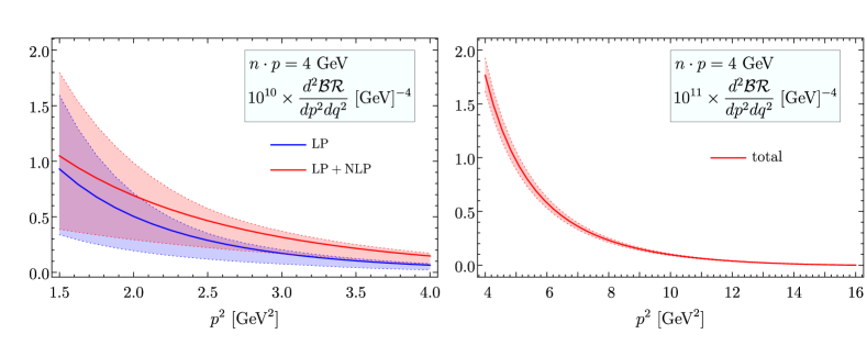
Figure 9: Theory predictions for the double differential branching fractions of the four-body leptonic $B$-meson decays with non-identical lepton flavours in the hard-collinear $p^{2}$ region (left panel) and in the hard $p^{2}$ region (right panel), where the numerical value of the large component of the virtual photon momentum is taken as $4\,{\rm GeV}$. The yielding uncertainty bands are obtained by adding the individual errors from varying all the theory input parameters in quadrature.

To facilitate the experimental explorations we proceed to construct the following weighted angular integrals for the five-fold differential decay width (118)

$$X(p^{2},q^{2})=\int_{-1}^{1}d\cos\theta_{1}\,\int_{-1}^{1}d\cos\theta_{2}\,\int_{0}^{2\pi}d\phi\,\frac{d^{5}\Gamma(B_{u}^{-}\to\ell^{\prime}\,\bar{\ell}^{\prime}\,\ell\,\bar{\nu}_{\ell})}{dp^{2}\,dq^{2}\,d\cos\theta_{1}\,d\cos\theta_{2}\,d\phi}\,\omega_{X}(p^{2},q^{2},\theta_{1},\theta_{2},\phi),\hskip 22.76228pt$$ (123)

to obtain the double differential distributions in the invariant masses $p^{2}$ and $q^{2}$. Adopting $\omega_{X}=1$ immediately leads to the familiar differential decay rate

$$\frac{d^{2}\Gamma}{dp^{2}\,dq^{2}}={1\over\tau_{B_{u}}}\,\frac{d^{2}{\cal BR}}{dp^{2}\,dq^{2}}={32\,\pi\over 9}\,{\cal N}(p^{2},q^{2})\,\left(4\,J_{1}+J_{2}\right)\,.$$ (124)

Inspecting the yielding predictions for the double differential branching fractions of the four-body leptonic $B$-meson decay processes displayed in Figure 9 implies that the newly obtained subleading power corrections computable in the perturbative factorization framework appear to enhance the counterpart LP contribution at the NLL accuracy significantly in the hard-collinear $p^{2}$ region (as large as ${\cal O}(40\,\%)$ enhancement at $p^{2}=2.5\,{\rm GeV^{2}}$ numerically) for the fixed value $n\cdot p=4\,{\rm GeV}$, where the substantial uncertainties represented by the blue and pink bands are due to the poorly constrained shape parameters of the two-particle and three-particle $B$-meson distribution amplitudes. By contrast, the resulting uncertainties for the differential branching fractions in the hard $p^{2}$ region turn out to be insignificant numerically (at the level of ${\cal O}(10\,\%)$), which can be traced back to the very independence of the HQET factorization formula (76) on the non-local hadronic quantities. Additionally, we predict the rapidly decreasing branching fractions in the kinematic regime $4.0\,{\rm GeV}^{2}\leq p^{2}\leq\,16.0\,{\rm GeV}^{2}$ when the invariant mass of the $\ell^{\prime}\bar{\ell}^{\prime}$ pair moves towards the higher values, which provides an explicit confirmation of the expected numerical features dictated by our power counting scheme (see [50] for an earlier discussion).

Along the same vein, we can readily define the non-vanishing angular asymmetries normalized to the differential decay width by taking the appropriate weight functions

$${\cal A}_{c2\theta_{1}} = \left[\frac{d^{2}\Gamma}{dp^{2}\,dq^{2}}\right]^{-1}\,\int_{-1}^{1}d\cos\theta_{1}\,\,{\rm sgn}\left(\cos(2\,\theta_{1})\right)\,\,\frac{d^{3}\Gamma(B_{u}^{-}\to\ell^{\prime}\,\bar{\ell}^{\prime}\,\ell\,\bar{\nu}_{\ell})}{dp^{2}\,dq^{2}\,d\cos\theta_{1}}$$

$$= 1-\frac{5}{2\,\sqrt{2}}+\frac{3}{\sqrt{2}}\,\frac{J_{1}}{4\,J_{1}+J_{2}}\,,$$

$${\cal A}_{c\theta_{2}} = \left[\frac{d^{2}\Gamma}{dp^{2}\,dq^{2}}\right]^{-1}\,\int_{-1}^{1}d\cos\theta_{2}\,\,{\rm sgn}\left(\cos(\theta_{2})\right)\,\,\frac{d^{3}\Gamma(B_{u}^{-}\to\ell^{\prime}\,\bar{\ell}^{\prime}\,\ell\,\bar{\nu}_{\ell})}{dp^{2}\,dq^{2}\,d\cos\theta_{2}}=\frac{3}{2}\,\frac{J_{3}}{4\,J_{1}+J_{2}}\,,$$

$${\cal A}_{s2\phi} = \left[\frac{d^{2}\Gamma}{dp^{2}\,dq^{2}}\right]^{-1}\,\int_{0}^{2\pi}\,\,{\rm sgn}\left(\sin(2\,\phi)\right)\,\,\frac{d^{3}\Gamma(B_{u}^{-}\to\ell^{\prime}\,\bar{\ell}^{\prime}\,\ell\,\bar{\nu}_{\ell})}{dp^{2}\,dq^{2}\,d\phi}=\frac{2}{\pi}\,\frac{J_{8}}{4\,J_{1}+J_{2}}\,,$$

$${\cal A}_{c2\phi} = \left[\frac{d^{2}\Gamma}{dp^{2}\,dq^{2}}\right]^{-1}\,\int_{0}^{2\pi}d\phi\,\,{\rm sgn}\left(\cos(2\,\phi)\right)\,\,\frac{d^{3}\Gamma(B_{u}^{-}\to\ell^{\prime}\,\bar{\ell}^{\prime}\,\ell\,\bar{\nu}_{\ell})}{dp^{2}\,dq^{2}\,d\phi}=\frac{2}{\pi}\,\frac{J_{9}}{4\,J_{1}+J_{2}}\,,$$

$${\cal A}_{s\phi,c\theta_{1}} = \left[\frac{d^{2}\Gamma}{dp^{2}\,dq^{2}}\right]^{-1}\,\int_{-1}^{1}d\cos\theta_{1}\,\int_{0}^{2\pi}d\phi\,\,{\rm sgn}\left(\sin(\phi)\right)\,{\rm sgn}\left(\cos(\theta_{1})\right)\,\,\frac{d^{4}\Gamma(B_{u}^{-}\to\ell^{\prime}\,\bar{\ell}^{\prime}\,\ell\,\bar{\nu}_{\ell})}{dp^{2}\,dq^{2}\,d\cos\theta_{1}\,d\phi}$$

$$= \frac{3}{4}\,\frac{J_{4}}{4\,J_{1}+J_{2}}\,,$$

$${\cal A}_{c\phi,c\theta_{1}} = \left[\frac{d^{2}\Gamma}{dp^{2}\,dq^{2}}\right]^{-1}\,\int_{-1}^{1}d\cos\theta_{1}\,\int_{0}^{2\pi}d\phi\,\,{\rm sgn}\left(\cos(\phi)\right)\,{\rm sgn}\left(\cos(\theta_{1})\right)\,\,\frac{d^{4}\Gamma(B_{u}^{-}\to\ell^{\prime}\,\bar{\ell}^{\prime}\,\ell\,\bar{\nu}_{\ell})}{dp^{2}\,dq^{2}\,d\cos\theta_{1}\,d\phi}$$

$$= \frac{3}{4}\,\frac{J_{6}}{4\,J_{1}+J_{2}}\,,$$

$${\cal A}_{s\phi,c\theta_{1},c\theta_{2}} = \left[\frac{d^{2}\Gamma}{dp^{2}\,dq^{2}}\right]^{-1}\,\int_{-1}^{1}d\cos\theta_{1}\,\int_{-1}^{1}d\cos\theta_{2}\,\int_{0}^{2\pi}d\phi\,\,$$

$$\times\,{\rm sgn}\left(\sin(\phi)\right)\,{\rm sgn}\left(\cos(\theta_{1})\right)\,{\rm sgn}\left(\cos(\theta_{2})\right)\,\,\frac{d^{5}\Gamma(B_{u}^{-}\to\ell^{\prime}\,\bar{\ell}^{\prime}\,\ell\,\bar{\nu}_{\ell})}{dp^{2}\,dq^{2}\,d\cos\theta_{1}\,d\cos\theta_{2}\,d\phi}$$

$$= \frac{2}{\pi}\,\frac{J_{5}}{4\,J_{1}+J_{2}}\,,$$

$${\cal A}_{c\phi,c\theta_{1},c\theta_{2}} = \left[\frac{d^{2}\Gamma}{dp^{2}\,dq^{2}}\right]^{-1}\,\int_{-1}^{1}d\cos\theta_{1}\,\int_{-1}^{1}d\cos\theta_{2}\,\int_{0}^{2\pi}d\phi\,\,$$ (125)

$$\times\,{\rm sgn}\left(\cos(\phi)\right)\,{\rm sgn}\left(\cos(\theta_{1})\right)\,{\rm sgn}\left(\cos(\theta_{2})\right)\,\,\frac{d^{5}\Gamma(B_{u}^{-}\to\ell^{\prime}\,\bar{\ell}^{\prime}\,\ell\,\bar{\nu}_{\ell})}{dp^{2}\,dq^{2}\,d\cos\theta_{1}\,d\cos\theta_{2}\,d\phi}$$

$$= \frac{2}{\pi}\,\frac{J_{7}}{4\,J_{1}+J_{2}}\,,$$

where the sign function reads ${\rm sgn}(\pm|x|)=\pm 1$ for any non-zero real number $x$. In contrast to the established angular observable ${\cal A}_{c\theta_{2}}$, we observe the vanishing single forward-backward asymmetry in the angle $\theta_{1}$ by taking advantage of the derived differential decay distribution (118) immediately. In order to determine the underlying mechanism for such an interesting discrepancy, we recall the well-known expression of the differential forward-backward asymmetry for the electroweak penguin $B\to K^{\ast}\ell\bar{\ell}$ decay process [80]

$${\cal A}_{\rm FB}(B\to K^{\ast}\ell\bar{\ell})\propto{\rm Re}\left(A_{\|,\,L}\,A_{\perp,\,L}^{\ast}\right)-\left(L\rightarrow R\right)\,,$$ (126)

where the four transversity amplitudes in the factorization approximation are given by

$$A_{\|,\,L(R)}\propto\left(C_{9}^{\rm eff}\mp C_{10}\right)\,\frac{V(q^{2})}{m_{B}+m_{K^{\ast}}}\,,\qquad A_{\perp,\,L(R)}\propto\left(C_{9}^{\rm eff}\mp C_{10}\right)\,\frac{A_{1}(q^{2})}{m_{B}-m_{K^{\ast}}}\,.$$ (127)

Confronting further the exclusive three-body $B\to W^{\ast}\,\ell^{\prime}\,\bar{\ell}^{\prime}$ decay amplitude

$${\cal M}(B\to W^{\ast}\,\ell^{\prime}\,\bar{\ell}^{\prime}) \propto \left[\bar{\ell}^{\prime}(p_{1})\,\gamma^{\nu}\,\ell^{\prime}(p_{2})\right]\,\bigg{\{}i\,\epsilon_{\mu\nu pv}\,\epsilon_{W^{\ast}}^{\mu}(q)\,F_{V}(p^{2},n\cdot p)+\epsilon_{W^{\ast}\nu}(q)\,v\cdot p\,F_{A}(p^{2},n\cdot p)$$ (128)

$$+\,q_{\nu}\,\frac{p\cdot\epsilon_{W^{\ast}}(q)}{m_{B}}\,\left[F_{1}(p^{2},n\cdot p)+{v\cdot p\over m_{B}}\,F_{3}(p^{2},n\cdot p)\right]\bigg{\}}\,,$$

with the analogous formula for the semileptonic $B\to K^{\ast}\ell\bar{\ell}$ decay amplitude

$${\cal M}(B\to K^{\ast}\,\ell\,\bar{\ell}) \propto \left[\bar{\ell}(q_{1})\,\gamma^{\mu}\,\left(C_{9}^{\rm eff}+C_{10}\,\gamma_{5}\right)\ell(q_{2})\right]\,\bigg{\{}i\,\epsilon_{\mu\nu pv}\,\epsilon_{K^{\ast}}^{\nu}(p)\,\left[\frac{2\,m_{B}}{m_{B}+m_{K^{\ast}}}V(q^{2})\,\right]$$ (129)

$$+\,\left[\epsilon_{K^{\ast}\mu}(p)-\frac{q\cdot\epsilon_{K^{\ast}}(p)}{q^{2}}\,q_{\mu}\right]\,\left(m_{B}+m_{K^{\ast}}\right)\,A_{1}(q^{2})+...\bigg{\}}\,,$$

we are then allowed to express the differential forward-backward asymmetry of $B\to W^{\ast}\,\ell^{\prime}\,\bar{\ell}^{\prime}$ from (126) analytically by implementing necessary replacements for the hadronic form factors and especially for the short-distance Wilson coefficients

$$C_{9}^{\rm eff}\to 1,\qquad C_{10}\to 0\,,$$ (130)

which leads to the vanishing result apparently due to an exact cancellation between the left-handed and right-handed contributions.

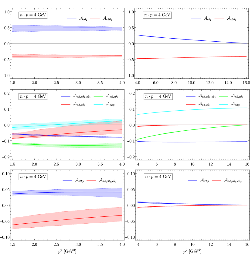
Figure 10: Theory predictions for the various angular asymmetries of the four-body leptonic $B$-meson decays with non-identical lepton flavours in the hard-collinear $p^{2}$ region (left panel) and in the hard $p^{2}$ region (right panel), where the numerical value of the large component of the virtual photon momentum is taken as $4\,{\rm GeV}$. The yielding uncertainty bands are obtained by adding the individual errors from varying all the theory input parameters in quadrature.

We now turn to present our predictions for the differential angular asymmetries of the four-body leptonic $B_{u}^{-}\to\ell^{\prime}\,\bar{\ell}^{\prime}\,\ell\,\bar{\nu}_{\ell}$ decays in the kinematic domain $1.5\,{\rm GeV^{2}}\leq p^{2}\leq 16.0\,{\rm GeV^{2}}$ in Figure 10, where the uncertainty bands are obtained by adding all the separate errors from the variations of the essential theory inputs in quadrature. The yielding pronounced results for the two angular observables ${\cal A}_{c2\theta_{1}}$ and ${\cal A}_{c\theta_{2}}$ in the hard-collinear $p^{2}$ region will evidently enable us to carry out the dedicated measurements with the encouraging precision at the LHCb and Belle II experiments. However, the four angular asymmetries ${\cal A}_{c2\phi}$, ${\cal A}_{s\phi,c\theta_{1}}$, ${\cal A}_{c\phi,c\theta_{1}}$ and ${\cal A}_{c\phi,c\theta_{1},c\theta_{2}}$ can reach at most ${\cal O}(10\,\%)$ numerically based upon our improved calculations for the radiative $B_{u}^{-}\to\gamma^{\ast}\,\ell\,\bar{\nu}_{\ell}$ decay form factors. In addition, the resulting predictions for the two remaining asymmetry observables ${\cal A}_{s2\phi}$ and ${\cal A}_{s\phi,c\theta_{1},c\theta_{2}}$ appear to be merely at the level of ${\cal O}(5\,\%)$, thus rendering their measurements considerably challenging for the ongoing collision experiments. It remains important to remark that the achieved uncertainties of the differential angular asymmetries for $1.5\,{\rm GeV^{2}}\leq p^{2}\leq 4.0\,{\rm GeV^{2}}$ are unsurprisingly improved, when compared with the obtained results for the differential branching fractions presented in Figure 9, on account of the substantial cancellation of the parametric uncertainties from the badly known $B$-meson distribution amplitudes in HQET.

Observables	$[t_{1},\,\,t_{2}]$	LP	Total	Uncertainties
	$({\rm GeV}^{2})$	(NLL)	(LP + NLP)	$\mu$	$\mu_{h1}$	$\widehat{\sigma}_{B_{u}}^{(1,\,2)}$	$\lambda_{B_{u}}$	$p^{2}_{\rm cut}$	$|V_{ub}|$
$\langle{{\cal BR}\,[t_{1},\,t_{2}]}\rangle\times 10^{9}$	$\left.\text{[1.5, }m_{B}^{2}\right]$	$0.88_{-0.37}^{+0.24}$	$1.23_{-0.52}^{+0.30}$	$\text{}_{-0.23}^{+0.06}$	$\text{}_{-0.19}^{+0.07}$	$\text{}_{-0.24}^{+0.21}$	$\text{}_{-0.32}^{+0.13}$	$\text{}_{-0.03}^{+0.05}$	$\text{}_{-0.10}^{+0.11}$
	$\left.\text{[2.0, }m_{B}^{2}\right]$	$0.57_{-0.20}^{+0.16}$	$0.83_{-0.29}^{+0.15}$	$\text{}_{-0.14}^{+0.04}$	$\text{}_{-0.11}^{+0.04}$	$\text{}_{-0.11}^{+0.02}$	$\text{}_{-0.17}^{+0.05}$	$\text{}_{-0.03}^{+0.05}$	$\text{}_{-0.07}^{+0.07}$
	$\left.\text{[3.0, }m_{B}^{2}\right]$	$0.32_{-0.09}^{+0.15}$	$0.42_{-0.09}^{+0.07}$	$\text{}_{-0.05}^{+0.02}$	$\text{}_{-0.03}^{+0.01}$	$\text{}_{-0.03}^{+0.00}$	$\text{}_{-0.04}^{+0.00}$	$\text{}_{-0.03}^{+0.05}$	$\text{}_{-0.04}^{+0.04}$
	$\left.\text{[4.0, }m_{B}^{2}\right]$	$0.24_{-0.08}^{+0.02}$	$0.24_{-0.04}^{+0.02}$	$\text{}_{-0.00}^{+0.00}$	$\text{}_{-0.00}^{+0.00}$	$\text{}_{-0.00}^{+0.00}$	$\text{}_{-0.00}^{+0.00}$	$\text{}_{-0.03}^{+0.00}$	$\text{}_{-0.02}^{+0.02}$
$\langle{{\cal A}_{c2\theta_{1}}\,[t_{1},\,t_{2}]}\rangle$	$\left.\text{[1.5, }m_{B}^{2}\right]$	$-0.38_{-0.08}^{+0.06}$	$-0.45_{-0.05}^{+0.04}$	$\text{}_{-0.01}^{+0.00}$	$\text{}_{-0.01}^{+0.00}$	$\text{}_{-0.03}^{+0.04}$	$\text{}_{-0.04}^{+0.01}$	$\text{}_{-0.02}^{+0.01}$	$-$
	$\left.\text{[2.0, }m_{B}^{2}\right]$	$-0.40_{-0.08}^{+0.05}$	$-0.46_{-0.05}^{+0.04}$	$\text{}_{-0.01}^{+0.00}$	$\text{}_{-0.01}^{+0.00}$	$\text{}_{-0.02}^{+0.02}$	$\text{}_{-0.03}^{+0.01}$	$\text{}_{-0.02}^{+0.01}$	$-$
	$\left.\text{[3.0, }m_{B}^{2}\right]$	$-0.47_{-0.07}^{+0.05}$	$-0.50_{-0.07}^{+0.06}$	$\text{}_{-0.01}^{+0.00}$	$\text{}_{-0.04}^{+0.00}$	$\text{}_{-0.01}^{+0.05}$	$\text{}_{-0.04}^{+0.01}$	$\text{}_{-0.04}^{+0.02}$	$-$
	$\left.\text{[4.0, }m_{B}^{2}\right]$	$-0.54_{-0.00}^{+0.05}$	$-0.54_{-0.00}^{+0.01}$	$\text{}_{-0.00}^{+0.00}$	$\text{}_{-0.00}^{+0.00}$	$\text{}_{-0.00}^{+0.00}$	$\text{}_{-0.00}^{+0.00}$	$\text{}_{-0.00}^{+0.01}$	$-$
$\langle{{\cal A}_{c\theta_{2}}\,[t_{1},\,t_{2}]}\rangle$	$\left.\text{[1.5, }m_{B}^{2}\right]$	$0.48_{-0.13}^{+0.09}$	$0.38_{-0.10}^{+0.07}$	$\text{}_{-0.03}^{+0.00}$	$\text{}_{-0.03}^{+0.01}$	$\text{}_{-0.05}^{+0.06}$	$\text{}_{-0.07}^{+0.03}$	$\text{}_{-0.03}^{+0.02}$	$-$
	$\left.\text{[2.0, }m_{B}^{2}\right]$	$0.43_{-0.13}^{+0.07}$	$0.36_{-0.10}^{+0.06}$	$\text{}_{-0.03}^{+0.00}$	$\text{}_{-0.03}^{+0.01}$	$\text{}_{-0.04}^{+0.04}$	$\text{}_{-0.07}^{+0.02}$	$\text{}_{-0.05}^{+0.03}$	$-$
	$\left.\text{[3.0, }m_{B}^{2}\right]$	$0.28_{-0.10}^{+0.08}$	$0.28_{-0.10}^{+0.05}$	$\text{}_{-0.03}^{+0.01}$	$\text{}_{-0.02}^{+0.01}$	$\text{}_{-0.02}^{+0.00}$	$\text{}_{-0.04}^{+0.01}$	$\text{}_{-0.08}^{+0.05}$	$-$
	$\left.\text{[4.0, }m_{B}^{2}\right]$	$0.17_{-0.01}^{+0.06}$	$0.17_{-0.01}^{+0.07}$	$\text{}_{-0.00}^{+0.00}$	$\text{}_{-0.00}^{+0.00}$	$\text{}_{-0.00}^{+0.00}$	$\text{}_{-0.00}^{+0.00}$	$\text{}_{-0.00}^{+0.07}$	$-$

Table 2: Theory predictions for the binned distributions of the branching fraction as well as the two angular asymmetries ${\cal A}_{c2\theta_{1}}$ and ${\cal A}_{c\theta_{2}}$ for the four-body leptonic $B$-meson decays with non-identical lepton flavours, where the numerically sizeable uncertainties from varying distinct input parameters are further displayed for completeness.

We are now in a position to investigate the binned distributions for both the branching fraction and the two promising angular asymmetries with the required kinematic cut on the large component of the off-shell photon momentum

$$\langle{{\cal BR}\,[t_{1},\,t_{2}]}\rangle = \tau_{B_{u}}\,\int_{t_{1}}^{t_{2}}\,dp^{2}\,\int_{0}^{(m_{B}-\sqrt{p^{2}})^{2}}\,dq^{2}\,\,\theta\left(n\cdot p-3\,{\rm GeV}\right)\,\frac{d^{2}\Gamma(B_{u}^{-}\to\ell^{\prime}\,\bar{\ell}^{\prime}\,\ell\,\bar{\nu}_{\ell})}{dp^{2}\,dq^{2}}\,,$$

$$\langle{{\cal A}_{c2\theta_{1}}\,[t_{1},\,t_{2}]}\rangle = \frac{\tau_{B_{u}}}{\langle{{\cal BR}\,[t_{1},\,t_{2}]}\rangle}\,\,\int_{t_{1}}^{t_{2}}\,dp^{2}\,\int_{0}^{(m_{B}-\sqrt{p^{2}})^{2}}\,dq^{2}\,\int_{-1}^{1}d\cos\theta_{1}\,\,{\rm sgn}\left(\cos(2\,\theta_{1})\right)\,$$

$$\times\,\theta\left(n\cdot p-3\,{\rm GeV}\right)\,\,\frac{d^{3}\Gamma(B_{u}^{-}\to\ell^{\prime}\,\bar{\ell}^{\prime}\,\ell\,\bar{\nu}_{\ell})}{dp^{2}\,dq^{2}\,d\cos\theta_{1}}\,,$$

$$\langle{{\cal A}_{c\theta_{2}}\,[t_{1},\,t_{2}]}\rangle = \frac{\tau_{B_{u}}}{\langle{{\cal BR}\,[t_{1},\,t_{2}]}\rangle}\,\,\int_{t_{1}}^{t_{2}}\,dp^{2}\,\int_{0}^{(m_{B}-\sqrt{p^{2}})^{2}}\,dq^{2}\,\int_{-1}^{1}d\cos\theta_{2}\,\,{\rm sgn}\left(\cos(\theta_{2})\right)\,$$ (131)

$$\times\,\theta\left(n\cdot p-3\,{\rm GeV}\right)\,\,\frac{d^{3}\Gamma(B_{u}^{-}\to\ell^{\prime}\,\bar{\ell}^{\prime}\,\ell\,\bar{\nu}_{\ell})}{dp^{2}\,dq^{2}\,d\cos\theta_{2}}\,,$$

where the conversion relations for the two scalar quantities $n\cdot p$ and $\bar{n}\cdot p$ are given by

$$n\cdot p=\frac{m_{B}^{2}-q^{2}+p^{2}+\sqrt{\lambda(m_{B}^{2},p^{2},q^{2})}}{2\,m_{B}},\qquad\bar{n}\cdot p=\frac{m_{B}^{2}-q^{2}+p^{2}-\sqrt{\lambda(m_{B}^{2},p^{2},q^{2})}}{2\,m_{B}}\,.\hskip 22.76228pt$$ (132)

We collect the numerical results for the LP and NLP computations of these binned observables in Table 2 subsequently with the combined theory uncertainties by adding all the individual errors in quadrature. Here the matching parameter $p^{2}_{\rm cut}=(4.0\pm 1.0)\,{\rm GeV^{2}}$ has been introduced to separate the hard and hard-collinear $p^{2}$ regimes such that the factorized expressions of the non-hadronic $B_{u}^{-}\to\gamma^{\ast}\,\ell\,\bar{\nu}_{\ell}$ form factors summarized in (68) are expected to be applicable for $p^{2}\in[1.5\,{\rm GeV^{2}},\,p^{2}_{\rm cut}]$, whereas the obtained HQET expressions shown in (76) will be employed for evaluating the angular functions $J_{i}$ in the kinematic interval $p^{2}_{\rm cut}\leq p^{2}\leq m_{B}^{2}$. Comparing the numerical predictions for the first and last bins of $\langle{{\cal BR}\,[t_{1},\,t_{2}]}\rangle$ indicates that the predicted hard-collinear contribution to the branching fraction in the bin $p^{2}\in[1.5\,{\rm GeV^{2}},\,4.0\,{\rm GeV^{2}}]$ is approximately a factor of three larger than the counterpart effect from the hard $p^{2}$ bin $[4.0\,{\rm GeV^{2}},\,m_{B}^{2}]$ within the sizeable theory uncertainties. Importantly, the factorizable subleading power corrections to the binned branching fractions of $[1.5\,{\rm GeV^{2}},\,2.0\,{\rm GeV^{2}}]$ and $[1.5\,{\rm GeV^{2}},\,4.0\,{\rm GeV^{2}}]$ with the SCET factorization technique will bring about the notable enhancements for the corresponding LP predictions, amounting to about ${\cal O}(30\,\%)$ and ${\cal O}(50\,\%)$ respectively. In addition, the yielding prediction of the binned decay rate $\langle{{\cal BR}\,[1.5\,{\rm GeV^{2}},\,2.0\,{\rm GeV^{2}}]}\rangle$ deduced from Table 2 is observed to be compatible with the previous calculation in the QCD factorization framework [50]. Apparently, the newly derived subleading power corrections can modify the corresponding LP predictions for the two binned asymmetries $\langle{{\cal A}_{c2\theta_{1}}\,[1.5\,{\rm GeV^{2}},\,m_{B}^{2}]}\rangle$ and $\langle{{\cal A}_{c\theta_{2}}\,[1.5\,{\rm GeV^{2}},\,m_{B}^{2}]}\rangle$ by an amount of approximately ${\cal O}(20\,\%)$. We further mention in passing that the fast-decreasing binned asymmetries $\langle{{\cal A}_{c\theta_{2}}\,[t_{1},\,m_{B}^{2}]}\rangle$ with the growing value of $t_{1}$ can be actually understood from the distinctive feature of the very differential angular asymmetry presented in Figure 10.

Finally we turn to explore the phenomenological opportunities for the four-body charged-current bottom-meson decays $B_{u}^{-}\to\ell^{\prime}\,\bar{\ell}^{\prime}\,\ell\,\bar{\nu}_{\ell}$ with identical lepton flavours $\ell^{\prime}=\ell$, which will become quite challenging experimentally due to the very appearance of the two indistinguishable like-sign leptons in the final state and especially the practical implementation of the essential cut on the virtual photon momentum for the sake of adopting the perturbative QCD factorization theorems. To this end, we will begin with the manifest expression of the full decay amplitude to lowest non-vanishing order in the electromagnetic interaction

$${\cal A}_{\rm tot}(B_{u}^{-}\to\ell\,\bar{\ell}\,\ell\,\bar{\nu}_{\ell}) = {\cal A}(B_{u}^{-}(p_{B})\to\gamma^{\ast}(p)(\to\ell(p_{1})\,\,\bar{\ell}(p_{2}))\,\,W^{\ast}(q)(\to\ell(q_{1})\,\bar{\nu}_{\ell}(q_{2})))$$ (133)

$$-\,{\cal A}(B_{u}^{-}(p_{B})\to\gamma^{\ast}(\tilde{p})(\to\ell(q_{1})\,\,\bar{\ell}(p_{2}))\,\,W^{\ast}(\tilde{q})(\to\ell(p_{1})\,\bar{\nu}_{\ell}(q_{2})))$$

$$\equiv {\cal A}_{\rm dir}(B_{u}^{-}\to\ell\,\bar{\ell}\,\ell\,\bar{\nu}_{\ell})-{\cal\tilde{A}}_{\rm exc}(B_{u}^{-}\to\ell\,\bar{\ell}\,\ell\,\bar{\nu}_{\ell})\,,$$

where the relative minus sign evidently stems from the Fermi-Dirac statistic for leptons. It is then straightforward to write down the desired differential decay width for the exclusive transition process $B_{u}^{-}\to\ell\,\bar{\ell}\,\ell\,\bar{\nu}_{\ell}$

$$d\Gamma(B_{u}^{-}\to\ell\,\bar{\ell}\,\ell\,\bar{\nu}_{\ell})=\left({1\over 2}\right)\,\frac{(2\,\pi)^{4}}{2\,m_{B}}\,\left[\left|{\cal A}_{\rm dir}\right|^{2}+|{\cal\tilde{A}}_{\rm exc}|^{2}-2\,{\rm Re}\left({\cal A}_{\rm dir}^{\ast}\,{\cal\tilde{A}}_{\rm exc}\right)\right]\,d\Phi_{4,\,\rm PS}\,,$$ (134)

where we have introduced the degeneracy factor $1/2$ to prevent the double counting of the identical particles in the final state and $d\Phi_{4,\,\rm PS}$ stands for an element of relativistically invariant four-body phase space

$$d\Phi_{4,\,\rm PS} = \frac{\lambda^{1/2}(m_{B}^{2},p^{2},q^{2})}{2^{8}\,\,(2\,\pi)^{10}\,m_{B}^{2}}\,\,\,dp^{2}\,dq^{2}\,d\cos\theta_{1}\,d\cos\theta_{2}\,d\phi$$ (135)

$$= \frac{\lambda^{1/2}(m_{B}^{2},\tilde{p}^{2},\tilde{q}^{2})}{2^{8}\,\,(2\,\pi)^{10}\,m_{B}^{2}}\,\,\,d\tilde{p}^{2}\,d\tilde{q}^{2}\,d\cos\tilde{\theta}_{1}\,d\cos\tilde{\theta}_{2}\,d\tilde{\phi}\,.$$

The explicit definitions of the two invariant masses $\tilde{p}^{2}$ and $\tilde{q}^{2}$ together with the three helicity angles $\tilde{\theta}_{1}$, $\tilde{\theta}_{2}$ and $\tilde{\phi}$ bear resemblance to the counterpart kinematic variables without a tilde symbol (see Appendix A for more details). The yielding full differential decay rate for the four-body leptonic $B$-meson decay with identical lepton flavours can be expressed as

$$\frac{d^{5}\Gamma(B_{u}^{-}\to\ell\,\bar{\ell}\,\ell\,\bar{\nu}_{\ell})}{dp^{2}\,dq^{2}\,d\cos\theta_{1}\,d\cos\theta_{2}\,d\phi}=\frac{G_{F}^{2}\,\alpha_{\rm em}^{2}\,|V_{ub}|^{2}}{2^{13}\,\pi^{4}}\,m_{B}^{3}\,\,\lambda^{1/2}(m_{B}^{2},p^{2},q^{2})\,\bigg{\{}\frac{1}{p^{4}}\,{\cal J}(p^{2},\,q^{2},\,\theta_{1},\,\theta_{2},\,\phi)\,$$

$$+\,\frac{1}{\tilde{p}^{4}}\,{\cal J}(\tilde{p}^{2},\,\tilde{q}^{2},\,\tilde{\theta}_{1},\,\tilde{\theta}_{2},\,\tilde{\phi})-{2\over p^{2}\,\tilde{p}^{2}}\,{\cal J}_{\rm int}(p^{2},\,\tilde{p}^{2},\,q^{2},\,\tilde{q}^{2},\,\theta_{1},\,\tilde{\theta}_{1},\,\theta_{2},\,\tilde{\theta}_{2},\,\phi,\,\tilde{\phi})\bigg{\}}\,,$$ (136)

where the angular distribution ${\cal J}$ of our interest has been previously derived in (119) and the emerged interference term ${\cal J}_{\rm int}$ remains invariant under the following transformation

$$p^{2}\leftrightarrow\tilde{p}^{2}\,,\qquad q^{2}\leftrightarrow\tilde{q}^{2}\,,\qquad\theta_{1}\leftrightarrow\tilde{\theta}_{1}\,,\qquad\theta_{2}\leftrightarrow\tilde{\theta}_{2}\,,\qquad\phi\leftrightarrow\tilde{\phi}\,.$$ (137)

We can readily identify the translation rules between the two complete sets of variables with and without a tilde for later convenience

$$\tilde{p}^{2} = \left({1\over 4}\right)\,\bigg{[}-\lambda^{1/2}(m_{B}^{2},p^{2},q^{2})\,\left(\cos\theta_{1}-\cos\theta_{2}\right)+(m_{B}^{2}-p^{2}-q^{2})\,\left(1-\cos\theta_{1}\cos\theta_{2}\right)$$

$$\hskip 36.98866pt+\,2\,\sqrt{p^{2}\,q^{2}}\,|\sin\theta_{1}\sin\theta_{2}|\,\cos\phi\bigg{]}\,,$$

$$\tilde{q}^{2} = \left({1\over 4}\right)\,\bigg{[}\lambda^{1/2}(m_{B}^{2},p^{2},q^{2})\,\left(\cos\theta_{1}-\cos\theta_{2}\right)+(m_{B}^{2}-p^{2}-q^{2})\,\left(1-\cos\theta_{1}\cos\theta_{2}\right)$$

$$\hskip 36.98866pt+\,2\,\sqrt{p^{2}\,q^{2}}\,|\sin\theta_{1}\sin\theta_{2}|\,\cos\phi\bigg{]}\,,$$

$$\cos\tilde{\theta}_{1} = \frac{1}{\lambda^{1/2}(m_{B}^{2},\tilde{p}^{2},\tilde{q}^{2})}\,\left[\frac{\lambda^{1/2}(m_{B}^{2},p^{2},q^{2})}{2}\,\left(\cos\theta_{1}+\cos\theta_{2}\right)-p^{2}+q^{2}\right]\,,$$

$$\cos\tilde{\theta}_{2} = \frac{1}{\lambda^{1/2}(m_{B}^{2},\tilde{p}^{2},\tilde{q}^{2})}\,\left[\frac{\lambda^{1/2}(m_{B}^{2},p^{2},q^{2})}{2}\,\left(\cos\theta_{1}+\cos\theta_{2}\right)+p^{2}-q^{2}\right]\,,$$

$$\sin\tilde{\phi} = -\frac{\lambda^{1/2}(m_{B}^{2},p^{2},q^{2})}{\lambda^{1/2}(m_{B}^{2},\tilde{p}^{2},\tilde{q}^{2})}\,\frac{\sqrt{p^{2}\,q^{2}}}{\sqrt{\tilde{p}^{2}\,\tilde{q}^{2}}}\,\left|\frac{\sin\theta_{1}\sin\theta_{2}}{\sin\tilde{\theta}_{1}\sin\tilde{\theta}_{2}}\right|\,\sin\phi\,,$$

$$\cos\tilde{\phi} = \frac{2\,(p^{2}+q^{2})-(m_{B}^{2}-\tilde{p}^{2}-\tilde{q}^{2})\,(1-\cos\tilde{\theta}_{1}\,\cos\tilde{\theta}_{2})}{2\,\sqrt{\tilde{p}^{2}\,\tilde{q}^{2}}\,\left|\sin\tilde{\theta}_{1}\sin\tilde{\theta}_{2}\right|}\,,$$ (138)

which will further enable us to derive the analytical form of ${\cal J}_{\rm int}$ in terms of the five independent variables $(p^{2},q^{2},\theta_{1},\theta_{2},\phi)$ collected in Appendix B.

As already pointed out in [50], the two resultant four-momenta $p=p_{1}+p_{2}$ and $\tilde{p}=q_{1}+p_{2}$ in this case cannot be distinguished experimentally. We will therefore implement both kinematic cuts on the light-cone components $n\cdot p$ and $n\cdot\tilde{p}$ simultaneously for constructing the accessible binned distributions in order to validate the established factorization formulae for the transverse and longitudinal $B_{u}^{-}\to\gamma^{\ast}\,W^{\ast}$ form factors. Moreover, the precise correspondence between the invariant mass of the off-shell photon and the kinematic variable $p^{2}$ does not hold anymore for the case of identical lepton flavours. Consequently, we propose to define the double-binned observables for the branching fraction and the angular asymmetries with the necessary kinematic constraints

$$\langle{{\cal BR}\,[t_{1},\,t_{2};\,\tilde{t}_{1},\,\tilde{t}_{2}]}\rangle = \tau_{B_{u}}\,\int_{0}^{m_{B}^{2}}\,dp^{2}\,\int_{0}^{(m_{B}-\sqrt{p^{2}})^{2}}\,dq^{2}\,\int_{-1}^{1}d\cos\theta_{1}\,\int_{-1}^{1}d\cos\theta_{2}\,\int_{0}^{2\pi}d\phi\,\,$$

$$\Theta_{\rm meas}(p^{2},\tilde{p}^{2},t_{1},t_{2},\tilde{t}_{1},\tilde{t}_{2})\,\,\frac{d^{5}\Gamma(B_{u}^{-}\to\ell\,\bar{\ell}\,\ell\,\bar{\nu}_{\ell})}{dp^{2}\,dq^{2}\,d\cos\theta_{1}\,d\cos\theta_{2}\,d\phi}\,,$$

$$\langle{{\cal A}_{c\theta_{1}+c\tilde{\theta}_{1}}\,[t_{1},\,t_{2};\,\tilde{t}_{1},\,\tilde{t}_{2}]}\rangle = \frac{\tau_{B_{u}}}{2\,\langle{{\cal BR}\,[t_{1},\,t_{2};\,\tilde{t}_{1},\,\tilde{t}_{2}]}\rangle}\,\,\int_{0}^{m_{B}^{2}}\,dp^{2}\,\int_{0}^{(m_{B}-\sqrt{p^{2}})^{2}}\,dq^{2}\,\int_{-1}^{1}d\cos\theta_{1}\,$$

$$\int_{-1}^{1}d\cos\theta_{2}\,\int_{0}^{2\pi}d\phi\,\left[{\rm sgn}\left(\cos(\theta_{1})\right)+{\rm sgn}\left(\cos(\tilde{\theta}_{1})\right)\right]\,$$

$$\times\,\Theta_{\rm meas}(p^{2},\tilde{p}^{2},t_{1},t_{2},\tilde{t}_{1},\tilde{t}_{2})\,\,\frac{d^{5}\Gamma(B_{u}^{-}\to\ell\,\bar{\ell}\,\ell\,\bar{\nu}_{\ell})}{dp^{2}\,dq^{2}\,d\cos\theta_{1}\,d\cos\theta_{2}\,d\phi}\,,$$

$$\langle{{\cal A}_{c2\theta_{1}+c2\tilde{\theta}_{1}}\,[t_{1},\,t_{2};\,\tilde{t}_{1},\,\tilde{t}_{2}]}\rangle = \frac{\tau_{B_{u}}}{2\,\langle{{\cal BR}\,[t_{1},\,t_{2};\,\tilde{t}_{1},\,\tilde{t}_{2}]}\rangle}\,\,\int_{0}^{m_{B}^{2}}\,dp^{2}\,\int_{0}^{(m_{B}-\sqrt{p^{2}})^{2}}\,dq^{2}\,\int_{-1}^{1}d\cos\theta_{1}\,\,$$

$$\int_{-1}^{1}d\cos\theta_{2}\,\int_{0}^{2\pi}d\phi\,\left[{\rm sgn}\left(\cos(2\theta_{1})\right)+{\rm sgn}\left(\cos(2\tilde{\theta}_{1})\right)\right]\,$$

$$\times\,\Theta_{\rm meas}(p^{2},\tilde{p}^{2},t_{1},t_{2},\tilde{t}_{1},\tilde{t}_{2})\,\,\frac{d^{5}\Gamma(B_{u}^{-}\to\ell\,\bar{\ell}\,\ell\,\bar{\nu}_{\ell})}{dp^{2}\,dq^{2}\,d\cos\theta_{1}\,d\cos\theta_{2}\,d\phi}\,,$$

$$\langle{{\cal A}_{c\theta_{2}+c\tilde{\theta}_{2}}\,[t_{1},\,t_{2};\,\tilde{t}_{1},\,\tilde{t}_{2}]}\rangle = \frac{\tau_{B_{u}}}{2\,\langle{{\cal BR}\,[t_{1},\,t_{2};\,\tilde{t}_{1},\,\tilde{t}_{2}]}\rangle}\,\,\int_{0}^{m_{B}^{2}}\,dp^{2}\,\int_{0}^{(m_{B}-\sqrt{p^{2}})^{2}}\,dq^{2}\,\int_{-1}^{1}d\cos\theta_{1}\,\,$$

$$\int_{-1}^{1}d\cos\theta_{2}\,\int_{0}^{2\pi}d\phi\,\left[{\rm sgn}\left(\cos(\theta_{2})\right)+{\rm sgn}\left(\cos(\tilde{\theta}_{2})\right)\right]$$

$$\times\,\Theta_{\rm meas}(p^{2},\tilde{p}^{2},t_{1},t_{2},\tilde{t}_{1},\tilde{t}_{2})\,\,\frac{d^{5}\Gamma(B_{u}^{-}\to\ell\,\bar{\ell}\,\ell\,\bar{\nu}_{\ell})}{dp^{2}\,dq^{2}\,d\cos\theta_{1}\,d\cos\theta_{2}\,d\phi}\,,$$

$$\langle{{\cal A}_{c\theta_{1},c\tilde{\theta}_{1}}\,[t_{1},\,t_{2};\,\tilde{t}_{1},\,\tilde{t}_{2}]}\rangle = \frac{\tau_{B_{u}}}{\langle{{\cal BR}\,[t_{1},\,t_{2};\,\tilde{t}_{1},\,\tilde{t}_{2}]}\rangle}\,\,\int_{0}^{m_{B}^{2}}\,dp^{2}\,\int_{0}^{(m_{B}-\sqrt{p^{2}})^{2}}\,dq^{2}\,\int_{-1}^{1}d\cos\theta_{1}\,\,$$

$$\int_{-1}^{1}d\cos\theta_{2}\,\int_{0}^{2\pi}d\phi\,\left[{\rm sgn}\left(\cos(\theta_{1})\right)\,{\rm sgn}\left(\cos(\tilde{\theta}_{1})\right)\right]$$

$$\times\,\Theta_{\rm meas}(p^{2},\tilde{p}^{2},t_{1},t_{2},\tilde{t}_{1},\tilde{t}_{2})\,\,\frac{d^{5}\Gamma(B_{u}^{-}\to\ell\,\bar{\ell}\,\ell\,\bar{\nu}_{\ell})}{dp^{2}\,dq^{2}\,d\cos\theta_{1}\,d\cos\theta_{2}\,d\phi}\,,$$

$$\langle{{\cal A}_{c2\theta_{1},c2\tilde{\theta}_{1}}\,[t_{1},\,t_{2};\,\tilde{t}_{1},\,\tilde{t}_{2}]}\rangle = \frac{\tau_{B_{u}}}{\langle{{\cal BR}\,[t_{1},\,t_{2};\,\tilde{t}_{1},\,\tilde{t}_{2}]}\rangle}\,\,\int_{0}^{m_{B}^{2}}\,dp^{2}\,\int_{0}^{(m_{B}-\sqrt{p^{2}})^{2}}\,dq^{2}\,\int_{-1}^{1}d\cos\theta_{1}\,\,$$

$$\int_{-1}^{1}d\cos\theta_{2}\,\int_{0}^{2\pi}d\phi\,\left[{\rm sgn}\left(\cos(2\theta_{1})\right)\,{\rm sgn}\left(\cos(2\tilde{\theta}_{1})\right)\right]\,$$

$$\times\,\Theta_{\rm meas}(p^{2},\tilde{p}^{2},t_{1},t_{2},\tilde{t}_{1},\tilde{t}_{2})\,\,\frac{d^{5}\Gamma(B_{u}^{-}\to\ell\,\bar{\ell}\,\ell\,\bar{\nu}_{\ell})}{dp^{2}\,dq^{2}\,d\cos\theta_{1}\,d\cos\theta_{2}\,d\phi}\,,$$

$$\langle{{\cal A}_{c\theta_{2},c\tilde{\theta}_{2}}\,[t_{1},\,t_{2};\,\tilde{t}_{1},\,\tilde{t}_{2}]}\rangle = \frac{\tau_{B_{u}}}{\langle{{\cal BR}\,[t_{1},\,t_{2};\,\tilde{t}_{1},\,\tilde{t}_{2}]}\rangle}\,\,\int_{0}^{m_{B}^{2}}\,dp^{2}\,\int_{0}^{(m_{B}-\sqrt{p^{2}})^{2}}\,dq^{2}\,\int_{-1}^{1}d\cos\theta_{1}\,\,$$ (139)

$$\int_{-1}^{1}d\cos\theta_{2}\,\int_{0}^{2\pi}d\phi\,\left[{\rm sgn}\left(\cos(\theta_{2})\right)\,{\rm sgn}\left(\cos(\tilde{\theta}_{2})\right)\right]\,$$

$$\times\,\Theta_{\rm meas}(p^{2},\tilde{p}^{2},t_{1},t_{2},\tilde{t}_{1},\tilde{t}_{2})\,\,\frac{d^{5}\Gamma(B_{u}^{-}\to\ell\,\bar{\ell}\,\ell\,\bar{\nu}_{\ell})}{dp^{2}\,dq^{2}\,d\cos\theta_{1}\,d\cos\theta_{2}\,d\phi}\,,$$

where the newly defined measurement function is explicitly given by

$$\Theta_{\rm meas} = \bigg{[}\theta(p^{2}-t_{1})\,\theta(t_{2}-p^{2})\,\theta(\tilde{p}^{2}-\tilde{t}_{1})\,\theta(\tilde{t}_{2}-\tilde{p}^{2})+\,\theta(p^{2}-\tilde{t}_{1})\,\theta(\tilde{t}_{2}-p^{2})\,\theta(\tilde{p}^{2}-t_{1})\,\theta(t_{2}-\tilde{p}^{2})$$

$$\hskip 8.5359pt-\,\theta(p^{2}-t_{1,\rm max})\,\theta(t_{2,\rm min}-p^{2})\,\theta(\tilde{p}^{2}-t_{1,\rm max})\,\theta(t_{2,\rm min}-\tilde{p}^{2})\bigg{]}$$

$$\times\,\bigg{[}\theta\left(n\cdot p-3\,{\rm GeV}\right)\,\theta\left(n\cdot\tilde{p}-3\,{\rm GeV}\right)\bigg{]}\,,$$

$$t_{1,\rm max} = {\rm max}\left\{t_{1},\,\tilde{t}_{1}\right\},\qquad t_{2,\rm min}={\rm min}\left\{t_{2},\,\tilde{t}_{2}\right\}.$$ (140)

It is important to remark that our definitions for the exclusive four-body $B_{u}^{-}\to\ell\,\bar{\ell}\,\ell\,\bar{\nu}_{\ell}$ decay observables differ from the previous strategies suggested in [50] on account of executing the essential kinematic cuts distinctly. As displayed in Table 3, the yielding double-binned branching fraction in the kinematic domain $\{p^{2}\,,\tilde{p}^{2}\}\in\left[1.5\,{\rm GeV^{2}},m_{B}^{2}\right]$ is predicted to be $(1.15^{+0.27}_{-0.49})\times 10^{-9}$, which lies well below the upper limit $1.6\times 10^{-8}$ for ${\cal BR}(B_{u}^{-}\to\mu^{+}\,\mu^{-}\,\mu^{-}\,\bar{\nu}_{\mu})$ reported by the LHCb Collaboration with the lowest of the two $\mu^{+}\,\mu^{-}$ invariant masses below $0.96\,{\rm GeV}^{2}$ [81]. Despite of the different implementations of kinematic constraints, our result for the partially integrated decay rate in the hard-collinear interval $\{p^{2}\,,\tilde{p}^{2}\}\in\left[1.5\,{\rm GeV^{2}},2.0\,{\rm GeV^{2}}\right]$ turns out to be comparable with the numerical value achieved in [50]. In particular, the subleading power corrections to the binned branching fractions of $\{p^{2}\,,\tilde{p}^{2}\}\in[1.5\,{\rm GeV^{2}},\,2.0\,{\rm GeV^{2}}]$ and $\{p^{2}\,,\tilde{p}^{2}\}\in[1.5\,{\rm GeV^{2}},\,4.0\,{\rm GeV^{2}}]$ tend to enhance the counterpart LP predictions significantly. Comparing the numerical predictions for $\langle{\cal BR}\rangle$ collected in Tables 2 and 3 further leads us to conclude that the coherent interference of the direct and exchange amplitudes merely generates the minor corrections to the double-binned branching fractions of $B_{u}^{-}\to\ell\,\bar{\ell}\,\ell\,\bar{\nu}_{\ell}$ for all the hard-collinear $\{p^{2}\,,\tilde{p}^{2}\}$-bins. Furthermore, our numerical computation indicates that only three of the six asymmetry observables $\langle{{\cal A}_{c2\theta_{1}+c2\tilde{\theta}_{1}}}\rangle$, $\langle{{\cal A}_{c\theta_{1},\,c\tilde{\theta}_{1}}}\rangle$ and $\langle{{\cal A}_{c\theta_{2},\,c\tilde{\theta}_{2}}}\rangle$ shown in Table 3 can reach ${\cal O}(50\,\%)$ in magnitudes and the yielding theory predictions suffer from the relatively lower uncertainties than those for $\langle{\cal BR}\rangle$, mainly due to the anticipated cancellation of the non-perturbative uncertainties from the HQET distribution amplitudes and of the perturbative uncertainties from the residual factorization/renormalization scale dependencies.

Observables	$[t_{1},\,\,t_{2}]$	LP	Total	Uncertainties
	$({\rm GeV}^{2})$	(NLL)	(LP + NLP)	$\mu$	$\mu_{h1}$	$\widehat{\sigma}_{B_{u}}^{(1,\,2)}$	$\lambda_{B_{u}}$	$p^{2}_{\rm cut}$	$|V_{ub}|$
$\langle{{\cal BR}\,[t_{1},\,t_{2};\,t_{1},\,t_{2}]}\rangle\times 10^{9}$	$\left.\text{[1.5, }m_{B}^{2}\right]$	$0.76_{-0.33}^{+0.22}$	$1.15_{-0.49}^{+0.27}$	$\text{}_{-0.21}^{+0.05}$	$\text{}_{-0.18}^{+0.07}$	$\text{}_{-0.22}^{+0.19}$	$\text{}_{-0.30}^{+0.12}$	$\text{}_{-0.02}^{+0.05}$	$\text{}_{-0.10}^{+0.10}$
	$\left.\text{[2.0, }m_{B}^{2}\right]$	$0.47_{-0.16}^{+0.16}$	$0.74_{-0.26}^{+0.12}$	$\text{}_{-0.12}^{+0.04}$	$\text{}_{-0.10}^{+0.04}$	$\text{}_{-0.10}^{+0.03}$	$\text{}_{-0.16}^{+0.06}$	$\text{}_{-0.02}^{+0.05}$	$\text{}_{-0.07}^{+0.07}$
	$\left.\text{[3.0, }m_{B}^{2}\right]$	$0.23_{-0.08}^{+0.13}$	$0.32_{-0.06}^{+0.06}$	$\text{}_{-0.03}^{+0.01}$	$\text{}_{-0.02}^{+0.01}$	$\text{}_{-0.02}^{+0.00}$	$\text{}_{-0.03}^{+0.00}$	$\text{}_{-0.02}^{+0.05}$	$\text{}_{-0.03}^{+0.03}$
	$\left.\text{[4.0, }m_{B}^{2}\right]$	$0.15_{-0.06}^{+0.02}$	$0.15_{-0.03}^{+0.02}$	$\text{}_{-0.00}^{+0.00}$	$\text{}_{-0.00}^{+0.00}$	$\text{}_{-0.00}^{+0.00}$	$\text{}_{-0.00}^{+0.00}$	$\text{}_{-0.02}^{+0.00}$	$\text{}_{-0.02}^{+0.02}$
$\langle{{\cal A}_{c2\theta_{1}+c2\tilde{\theta}_{1}}\,[t_{1},\,t_{2};\,t_{1},\,t_{2}]}\rangle$	$\left.\text{[1.5, }m_{B}^{2}\right]$	$-0.54^{+0.03}_{-0.09}$	$-0.60^{+0.03}_{-0.05}$	${}^{+0.00}_{-0.02}$	${}^{+0.00}_{-0.01}$	${}^{+0.03}_{-0.02}$	${}^{+0.01}_{-0.03}$	${}^{+0.00}_{-0.01}$	$-$
	$\left.\text{[2.0, }m_{B}^{2}\right]$	$-0.64^{+0.04}_{-0.05}$	$-0.67^{+0.02}_{-0.04}$	${}^{+0.00}_{-0.01}$	${}^{+0.00}_{-0.01}$	${}^{+0.01}_{-0.02}$	${}^{+0.01}_{-0.03}$	${}^{+0.00}_{-0.01}$	$-$
	$\left.\text{[3.0, }m_{B}^{2}\right]$	$-0.70^{+0.02}_{-0.05}$	$-0.72^{+0.03}_{-0.01}$	${}^{+0.01}_{-0.01}$	${}^{+0.01}_{-0.00}$	${}^{+0.01}_{-0.00}$	${}^{+0.01}_{-0.00}$	${}^{+0.02}_{-0.00}$	$-$
	$\left.\text{[4.0, }m_{B}^{2}\right]$	$-0.69^{+0.03}_{-0.02}$	$-0.70^{+0.03}_{-0.00}$	${}^{+0.00}_{-0.00}$	${}^{+0.01}_{-0.00}$	${}^{+0.00}_{-0.00}$	${}^{+0.00}_{-0.00}$	${}^{+0.03}_{-0.00}$	$-$
$\langle{{\cal A}_{c\theta_{1},\,c\tilde{\theta}_{1}}\,[t_{1},\,t_{2};\,t_{1},\,t_{2}]}\rangle$	$\left.\text{[1.5, }m_{B}^{2}\right]$	$0.25^{+0.09}_{-0.05}$	$0.29^{+0.05}_{-0.04}$	${}^{+0.03}_{-0.01}$	${}^{+0.02}_{-0.01}$	${}^{+0.01}_{-0.03}$	${}^{+0.03}_{-0.02}$	${}^{+0.02}_{-0.00}$	$-$
	$\left.\text{[2.0, }m_{B}^{2}\right]$	$0.31^{+0.07}_{-0.06}$	$0.33^{+0.04}_{-0.06}$	${}^{+0.02}_{-0.01}$	${}^{+0.02}_{-0.01}$	${}^{+0.00}_{-0.01}$	${}^{+0.02}_{-0.01}$	${}^{+0.02}_{-0.00}$	$-$
	$\left.\text{[3.0, }m_{B}^{2}\right]$	$0.42^{+0.03}_{-0.04}$	$0.40^{+0.04}_{-0.03}$	${}^{+0.01}_{-0.01}$	${}^{+0.01}_{-0.01}$	${}^{+0.01}_{-0.00}$	${}^{+0.02}_{-0.00}$	${}^{+0.03}_{-0.02}$	$-$
	$\left.\text{[4.0, }m_{B}^{2}\right]$	$0.50^{+0.02}_{-0.01}$	$0.50^{+0.02}_{-0.01}$	${}^{+0.00}_{-0.00}$	${}^{+0.01}_{-0.00}$	${}^{+0.00}_{-0.00}$	${}^{+0.00}_{-0.00}$	${}^{+0.00}_{-0.01}$	$-$
$\langle{{\cal A}_{c\theta_{2},\,c\tilde{\theta}_{2}}\,[t_{1},\,t_{2};\,t_{1},\,t_{2}]}\rangle$	$\left.\text{[1.5, }m_{B}^{2}\right]$	$0.24^{+0.10}_{-0.05}$	$0.27^{+0.09}_{-0.02}$	${}^{+0.03}_{-0.00}$	${}^{+0.03}_{-0.00}$	${}^{+0.04}_{-0.01}$	${}^{+0.06}_{-0.01}$	${}^{+0.03}_{-0.02}$	$-$
	$\left.\text{[2.0, }m_{B}^{2}\right]$	$0.32^{+0.06}_{-0.10}$	$0.31^{+0.08}_{-0.02}$	${}^{+0.04}_{-0.00}$	${}^{+0.04}_{-0.00}$	${}^{+0.03}_{-0.00}$	${}^{+0.03}_{-0.00}$	${}^{+0.03}_{-0.02}$	$-$
	$\left.\text{[3.0, }m_{B}^{2}\right]$	$0.44^{+0.04}_{-0.03}$	$0.42^{+0.03}_{-0.02}$	${}^{+0.02}_{-0.01}$	${}^{+0.01}_{-0.01}$	${}^{+0.00}_{-0.00}$	${}^{+0.01}_{-0.00}$	${}^{+0.02}_{-0.02}$	$-$
	$\left.\text{[4.0, }m_{B}^{2}\right]$	$0.52^{+0.04}_{-0.00}$	$0.52^{+0.00}_{-0.02}$	${}^{+0.00}_{-0.00}$	${}^{+0.00}_{-0.01}$	${}^{+0.00}_{-0.00}$	${}^{+0.00}_{-0.00}$	${}^{+0.00}_{-0.00}$	$-$

Table 3: Theory predictions for the binned distributions of the branching fraction $\langle{\cal BR}\rangle$ as well as the three angular asymmetries $\langle{{\cal A}_{c2\theta_{1}+c2\tilde{\theta}_{1}}}\rangle$, $\langle{{\cal A}_{c\theta_{1},\,c\tilde{\theta}_{1}}}\rangle$ and $\langle{{\cal A}_{c\theta_{2},\,c\tilde{\theta}_{2}}}\rangle$ for the four-body leptonic $B$-meson decays with identical lepton flavours, where the numerically sizeable uncertainties from varying distinct input parameters are further displayed for completeness.

6 Summary and conclusions

In this paper we have performed the improved QCD calculations of the exclusive radiative $B_{u}^{-}\to\gamma^{\ast}\,\ell\,\bar{\nu}_{\ell}$ form factors with an off-shell photon carrying either the hard-collinear momentum $p_{\mu}\sim m_{b}\,(1,\lambda^{2},\lambda)$ or the hard momentum $p_{\mu}\sim m_{b}\,(1,1,1)$ by taking advantage of the modern SCET factorization program and the traditional local OPE technique, respectively. Applying further the renormalized jet functions in the factorized expressions of the analogous $B$-meson-to-vacuum correlations for constructing the light-cone sum rules of the semileptonic $B\to V$ transition form factors [16] as well as the hadronic photon correction to the on-shell $B\to\gamma$ form factors [7], we constructed explicitly the soft-collinear factorization formulae for both the transverse and longitudinal $B\to\gamma^{\ast}\,\ell\,\bar{\nu}_{\ell}$ form factors at the NLL accuracy in the hard-collinear $p^{2}$-region with the aid of the Ward-Takahashi identities due to the ${\rm U_{em}}(1)$ gauge symmetry and the standard momentum-space RG formalism. Subsequently, we evaluated the distinct subleading-power contributions to the generalized $B\to\gamma^{\ast}\,W^{\ast}$ form factors at $p^{2}\sim{\cal O}(m_{b}\,\Lambda_{\rm QCD})$ from expanding the hard-collinear quark propagator beyond the LP approximation, from the two-particle and three-particle higher-twist HQET distribution amplitudes, from the “kinematic” power corrections suppressed by the small (but non-vanishing) component of the virtual photon momentum, and from the energetic photon radiation off the bottom quark at LO in the strong coupling constant. The yielding HQET factorization formulae of the non-hadronic $B\to\gamma^{\ast}$ form factors were then derived in the NLL approximation for $p^{2}\sim{\cal O}(m_{b}^{2})$ with the effective decay constant $\tilde{f}_{B}$ encoding the non-perturbative dynamics of the composite bottom-meson system.

Having at our disposal the desired expressions for the exclusive $B\to\gamma^{\ast}\,\ell\,\bar{\nu}_{\ell}$ decay form factors, we proceeded to explore their numerical implications with the three-parameter ansatz for the essential $B$-meson distribution amplitudes whose RG evolution behaviours can be determined analytically in terms of hypergeometric functions at one-loop order [8]. It has been observed that the resulting non-local power corrections from the subleading terms in the expanded hard-collinear quark propagator can shift the counterpart LP predictions by an amount of approximately $(20-30)\%$ in magnitudes in the kinematic domain $p^{2}\in[1.5,\,4.0]\,{\rm GeV^{2}}$. In particular, the predicted LP contribution to the vector form factor $|F_{V}|$ appeared to develop the yet stronger sensitivity on the inverse moment $\lambda_{B_{u}}$ in comparison with the obtained longitudinal form factor $\left|\lambda\,\left(\hat{F}_{1}+{v\cdot p\over m_{B}}\,\hat{F}_{3}\right)\right|$, which can be traced back to the quite distinct asymptotic behaviours of the two HQET distribution amplitudes $\phi_{B}^{\pm}(\omega,\mu)$ at small partonic momentum $\omega$. Unsurprisingly, the generalized radiative $B\to\gamma^{\ast}\,W^{\ast}$ form factors dependent on the invariant masses of both $\gamma^{\ast}$ and $W^{\ast}$ turned out to be rather sensitive to the precise shape of the $B$-meson distribution amplitudes. By contrast, the resulting theory predictions for such non-hadronic decay form factors in the hard $p^{2}$-regime suffered from the enormously reduced uncertainties due to the apparent independence of the non-perturbative light-ray distributions. We then turned to investigate systematically the angular observables for the four-body leptonic decays $B_{u}^{-}\to\ell^{\prime}\,\bar{\ell}^{\prime}\,\ell\,\bar{\nu}_{\ell}$ with non-identical lepton flavours $\ell\neq\ell^{\prime}$ and (more complicated) identical ones $\ell=\ell^{\prime}$. Our numerical results indicated that the dominant contribution to the branching fraction of $B_{u}^{-}\to\ell^{\prime}\,\bar{\ell}^{\prime}\,\ell\,\bar{\nu}_{\ell}$ indeed arises from the hard-collinear $p^{2}$-region rather than from the kinematic regime of $p_{\mu}\sim m_{b}\,(1,1,1)$ as anticipated by the power-counting analysis. It is also interesting to remark that the newly computed subleading power contributions to the binned branching fractions resulted in the sizeable enhancements of the corresponding LP computations based upon the SCET factorization approach. Additionally, the two promising asymmetry observables $\langle{{\cal A}_{c2\theta_{1}}\,[t_{1}\,t_{2}]}\rangle$ and $\langle{{\cal A}_{c\theta_{2}}\,[t_{1}\,t_{2}]}\rangle$ for non-identical lepton flavours have been predicted to be as large as ${\cal O}(20-50)\%$ for all the selected $p^{2}$-bins with the substantially improved precision. Furthermore, we quote our theory prediction for the double-binned branching fraction of $B_{u}^{-}\to\ell\,\bar{\ell}\,\ell\,\bar{\nu}_{\ell}$ as $(1.15^{+0.27}_{-0.49})\times 10^{-9}$ in the kinematic interval $\{p^{2}\,,\tilde{p}^{2}\}\in\left[1.5\,{\rm GeV^{2}},m_{B}^{2}\right]$ with the additional cuts on the large light-cone components of the two indistinguishable lepton-pair momenta $n\cdot p\geq 3\,{\rm GeV}$ and $n\cdot\tilde{p}\geq 3\,{\rm GeV}$.

Confronting our theory predictions for the binned decay rates and the angular asymmetries with the upcoming dedicated measurements at the LHCb and Belle II experiments will be evidently beneficial for advancing our knowledge of the poorly constrained $B$-meson distribution amplitudes in a complementary manner to the previous determination from the exclusive radiative $B\to\gamma\ell\bar{\nu}_{\ell}$ decays. In this respect, it will be in high demand to carry out a global fit of all the key exclusive channels including further a variety of semileptonic and nonleptonic bottom-meson decays for the sake of obtaining the more stringent constraints on the fundamental HQET distribution amplitudes (see also [82] for an alternative strategy). Further theoretical investigations of the non-hadronic $B\to\gamma^{\ast}\,W^{\ast}$ form factors can be also pursued by constructing the soft-collinear factorization formulae for their subleading power contributions systematically with the ${\rm QCD}\rightarrow\rm{SCET_{I}}\rightarrow\rm{SCET_{II}}$ matching procedure [83].

Acknowledgements

We are grateful to Alexander Khodjamirian for illuminating discussions. C.W is supported in part by the National Natural Science Foundation of China with Grant No. 12105112 and the Natural Science Foundation of Jiangsu Education Committee with Grant No. 21KJB140027. Y.M.W acknowledges support from the National Natural Science Foundation of China with Grant No. 11735010 and 12075125, and the Natural Science Foundation of Tianjin with Grant No. 19JCJQJC61100. Y.B.W is supported in part by the Alexander-von-Humboldt Stiftung.

Appendix A Kinematics for the four-body decays $B_{u}^{-}\to\ell^{\prime}\,\bar{\ell}^{\prime}\,\ell\,\bar{\nu}_{\ell}$

In this appendix, we will begin with the essential kinematics for the four-body leptonic decays $B_{u}^{-}(p_{B})\to\gamma^{\ast}(p)(\to\ell^{\prime}(p_{1})\,\,\bar{\ell}^{\prime}(p_{2}))\,W^{\ast}(q)(\to\ell(q_{1})\,\bar{\nu}_{\ell}(q_{2}))$ with non-identical lepton flavours $\ell^{\prime}\neq\ell$. Following the discussion for the exclusive $B\to K^{\ast}(\to K\pi)\,\ell\,\bar{\ell}$ decays [80], it is customary and convenient to express the full differential decay distribution of $B_{u}^{-}\to\ell^{\prime}\,\bar{\ell}^{\prime}\,\ell\,\bar{\nu}_{\ell}$ in terms of the five kinematic variables: the two invariant masses $p^{2}$ and $q^{2}$, the helicity angles $\theta_{1}$ and $\theta_{2}$, as well as the azimuthal angle $\phi$ (see Figure 11).

More explicitly, we choose the $z$-axis along the flight direction of the off-shell photon momentum $\bf{p}$ in the $B$-meson rest frame. The angle $\theta_{1}$ is then defined as the angle between the $\ell^{\prime-}$ direction of flight and the $z$-axis in the dilepton rest frame. As a consequence, the leptonic momenta in the dilepton rest frame ($2\,\ell^{\prime}$-RF) in the massless limit are given by

$$p_{1}|_{2\,\ell^{\prime}-{\rm RF}} = {\sqrt{p^{2}}\over 2}\,(1,\,\sin\theta_{1},\,0,\cos\theta_{1})\,,$$

$$p_{2}|_{2\,\ell^{\prime}-{\rm RF}} = {\sqrt{p^{2}}\over 2}\,(1,\,-\sin\theta_{1},\,0,-\cos\theta_{1})\,.$$ (141)

In addition, $\theta_{2}$ is the angle between the $\ell^{-}$-momentum $\bf{q_{1}}$ and the negative $z$ direction in the $W^{\ast}$-boson rest frame. The azimuthal angle $\phi$ is defined by the relative angle between the decay plane of the $\ell^{\prime}\bar{\ell^{\prime}}$ system and the $\ell\,\bar{\nu}_{\ell}$ decay plane. Accordingly, the two momenta $q_{1}$ and $q_{2}$ in the $\ell\,\bar{\nu}_{\ell}$ rest frame ($\ell\,\bar{\nu}_{\ell}$-RF) can be written as

$$q_{1}|_{\ell\,\bar{\nu}_{\ell}-{\rm RF}} = {\sqrt{q^{2}}\over 2}\,(1,\,\sin\theta_{2}\,\cos\phi,\,\sin\theta_{2}\,\sin\phi,\,-\cos\theta_{2})\,,$$

$$q_{2}|_{\ell\,\bar{\nu}_{\ell}-{\rm RF}} = {\sqrt{q^{2}}\over 2}\,(1,\,-\sin\theta_{2}\,\cos\phi,\,-\sin\theta_{2}\,\sin\phi,\,\cos\theta_{2})\,.$$ (142)

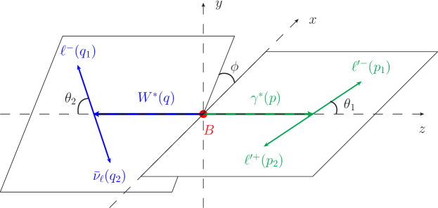
Figure 11: Kinematics of the four-body leptonic decay $B_{u}^{-}\to\ell^{\prime}\,\bar{\ell}^{\prime}\,\ell\,\bar{\nu}_{\ell}$.

Now we proceed to investigate the more complicated kinematics for the exclusive four-body bottom-meson decays $B_{u}^{-}\to\ell^{\prime}\,\bar{\ell}^{\prime}\,\ell\,\bar{\nu}_{\ell}$ with identical lepton flavours $\ell^{\prime}=\ell$. In order to evaluate the so-called exchange amplitude ${\cal\tilde{A}}_{\rm exc}$ displayed in (133), it proves more convenient to introduce further the two invariant masses in the following

$$\tilde{p}^{2}=(q_{1}+p_{2})^{2}\,,\qquad\tilde{q}^{2}=(p_{1}+q_{2})^{2}\,,$$ (143)

as well as the three alternative helicity angles $\tilde{\theta}_{1}$, $\tilde{\theta}_{2}$ and $\tilde{\phi}$ such that

$$q_{1}|_{\ell\,\bar{\ell}^{\prime}-{\rm RF}} = {\sqrt{\tilde{p}^{2}}\over 2}\,(1,\,\sin\tilde{\theta}_{1},\,0,\cos\tilde{\theta}_{1})\,,$$

$$p_{2}|_{\ell\,\bar{\ell}^{\prime}-{\rm RF}} = {\sqrt{\tilde{p}^{2}}\over 2}\,(1,\,-\sin\tilde{\theta}_{1},\,0,-\cos\tilde{\theta}_{1})\,,$$ (144)

correspond to the four-momenta of the final-state leptons from the cascade decay process $\gamma^{\ast}(\tilde{p})\to\ell(q_{1})\,\bar{\ell}^{\prime}(p_{2})$ in the dilepton rest frame ($\ell\,\bar{\ell}^{\prime}$-RF), and

$$p_{1}|_{\ell^{\prime}\,\bar{\nu}_{\ell}-{\rm RF}} = {\sqrt{\tilde{q}^{2}}\over 2}\,(1,\,\sin\tilde{\theta}_{2}\,\cos\tilde{\phi},\,\sin\tilde{\theta}_{2}\,\sin\tilde{\phi},\,-\cos\tilde{\theta}_{2})\,,$$

$$q_{2}|_{\ell^{\prime}\,\bar{\nu}_{\ell}-{\rm RF}} = {\sqrt{\tilde{q}^{2}}\over 2}\,(1,\,-\sin\tilde{\theta}_{2}\,\cos\tilde{\phi},\,-\sin\tilde{\theta}_{2}\,\sin\tilde{\phi},\,\cos\tilde{\theta}_{2})\,,$$ (145)

coincide with the four-momenta of the final-state particles produced from the cascade weak transition $W^{\ast}(\tilde{q})\to\ell^{\prime}(p_{1})\,\bar{\nu}_{\ell}(q_{2})$ in the $\ell^{\prime}\,\bar{\nu}_{\ell}$ rest frame ($\ell^{\prime}\,\bar{\nu}_{\ell}$-RF), respectively.

Appendix B Explicit expressions for the angular function ${\cal J}_{\rm int}$

Here we will present the detailed expressions for ${\cal J}_{\rm int}$ entering the differential decay distribution of the exclusive four-body bottom-meson decay with identical lepton flavours (136) due to the coherent interference of the direct and exchange amplitudes. By analogy with the result (119) for the non-hadronic process $B_{u}^{-}\to\ell^{\prime}\,\bar{\ell}^{\prime}\,\ell\,\bar{\nu}_{\ell}$ with $\ell^{\prime}\neq\ell$, the yielding decomposition for the intricate angular function ${\cal J}_{\rm int}$ can be cast in the form of

$${\cal J}_{\rm int} = \tilde{J}_{1}\,\left(\cos\theta_{1}+\cos\theta_{2}\right)^{2}+\tilde{J}_{2}\,\left(\cos\theta_{1}+\cos\theta_{2}\right)\,\left(1+\cos\theta_{1}\,\cos\theta_{2}\right)$$ (146)

$$+\,\tilde{J}_{3}\,\left(\cos\theta_{1}+\cos\theta_{2}\right)\,\sin^{2}\theta_{1}\,\sin^{2}\theta_{2}+\tilde{J}_{4}\,\left(\cos\theta_{1}+\cos\theta_{2}\right)\,\left(\sin^{2}\theta_{1}+\sin^{2}\theta_{2}\right)$$

$$+\,\tilde{J}_{5}\,\left(1+\cos\theta_{1}\,\cos\theta_{2}\right)\,\left(\sin^{2}\theta_{1}+\sin^{2}\theta_{2}\right)+\,\tilde{J}_{6}\,\sin^{2}\theta_{1}\,\sin^{2}\theta_{2}$$

$$+\,\tilde{J}_{7}\,\left(\cos\theta_{1}+\cos\theta_{2}\right)\,\sin\theta_{1}\,\sin\theta_{2}\,\sin\phi$$

$$+\,\tilde{J}_{8}\,\left(\cos\theta_{1}+\cos\theta_{2}\right)\,\left(1+\cos\theta_{1}\,\cos\theta_{2}\right)\,\sin\theta_{1}\,\sin\theta_{2}\,\sin\phi$$

$$+\,\tilde{J}_{9}\,\left(1+\cos\theta_{1}\,\cos\theta_{2}\right)\,\sin\theta_{1}\,\sin\theta_{2}\,\sin\phi$$

$$+\,\tilde{J}_{10}\,\sin\theta_{1}\,\sin\theta_{2}\,\left(\sin^{2}\theta_{1}+\sin^{2}\theta_{2}\right)\,\sin\phi$$

$$+\,\tilde{J}_{11}\,\left(\cos\theta_{1}+\cos\theta_{2}\right)\,\sin\theta_{1}\,\sin\theta_{2}\,\cos\phi$$

$$+\,\tilde{J}_{12}\,\left(1+\cos\theta_{1}\,\cos\theta_{2}\right)\,\sin\theta_{1}\,\sin\theta_{2}\,\cos\phi$$

$$+\,\tilde{J}_{13}\,\left(\cos\theta_{1}+\cos\theta_{2}\right)^{2}\,\sin\theta_{1}\,\sin\theta_{2}\,\cos\phi$$

$$+\,\tilde{J}_{14}\,\left(\cos\theta_{1}+\cos\theta_{2}\right)\,\sin(2\theta_{1})\,\sin(2\theta_{2})\,\cos\phi$$

$$+\,\tilde{J}_{15}\,\sin^{2}\theta_{1}\,\sin^{2}\theta_{2}\,\sin(2\phi)+\tilde{J}_{16}\,\left(\cos\theta_{1}+\cos\theta_{2}\right)\,\sin^{2}\theta_{1}\,\sin^{2}\theta_{2}\,\sin(2\phi)$$

$$+\,\tilde{J}_{17}\,\sin^{2}\theta_{1}\,\sin^{2}\theta_{2}\,\cos(2\phi)+\tilde{J}_{18}\,\left(\cos\theta_{1}+\cos\theta_{2}\right)\,\sin^{2}\theta_{1}\,\sin^{2}\theta_{2}\,\cos(2\phi)\,.$$

The coefficient functions $\tilde{J}_{i}$ (with $i=1,2,...18$) can be further expressed in terms of the generalized $B_{u}^{-}\to\gamma^{\ast}\,W^{\ast}$ transition form factors $F_{k}\equiv F_{k}(p^{2},q^{2})$ and ${\mathbb{F}}_{k}\equiv F_{k}(\tilde{p}^{2},\tilde{q}^{2})$ together with the suitable kinematic functions ($k=V,A,\parallel$)

$$\tilde{J}_{1} = -\,\,\hat{p}^{2}\,\hat{q}^{2}\,(1+\hat{p}^{2}-\hat{q}^{2})\,\,{\rm Re}\left[(1+\hat{\tilde{p}}^{2}-\hat{\tilde{q}}^{2})\,F_{A}\,{\mathbb{F}}_{A}^{\ast}+F_{A}\,{\mathbb{F}}_{\|}^{\ast}\right]\,,$$

$$\tilde{J}_{2} = -\,\,\hat{p}^{2}\,\hat{q}^{2}\,\lambda^{1/2}(1,\hat{p}^{2},\hat{q}^{2})\,\,{\rm Re}\left[(1+\hat{\tilde{p}}^{2}-\hat{\tilde{q}}^{2})\,F_{V}\,{\mathbb{F}}_{A}^{\ast}+F_{V}\,{\mathbb{F}}_{\|}^{\ast}\right]\,,$$

$$\tilde{J}_{3} = -{1\over 8}\,\,\lambda^{3/2}(1,\hat{p}^{2},\hat{q}^{2})\,\bigg{\{}\left[1+\frac{6\,\hat{p}^{2}\,\hat{q}^{2}}{\lambda(1,\hat{p}^{2},\hat{q}^{2})}\right]\,(1+\hat{p}^{2}-\hat{q}^{2})\,{\rm Re}\left(F_{A}\,{\mathbb{F}}_{V}^{\ast}\right)$$

$$+\,(1-\hat{p}^{2}-\hat{q}^{2})\,\,{\rm Re}\left(F_{\|}\,{\mathbb{F}}_{V}^{\ast}\right)\bigg{\}}\,,$$

$$\tilde{J}_{4} = {1\over 2}\,\,\hat{p}^{2}\,\hat{q}^{2}\,(1+\hat{p}^{2}-\hat{q}^{2})\,\lambda^{1/2}(1,\hat{p}^{2},\hat{q}^{2})\,\,{\rm Re}\left(F_{A}\,{\mathbb{F}}_{V}^{\ast}\right)\,,$$

$$\tilde{J}_{5} = {1\over 2}\,\,\hat{p}^{2}\,\hat{q}^{2}\,\lambda(1,\hat{p}^{2},\hat{q}^{2})\,\,{\rm Re}\left(F_{V}\,{\mathbb{F}}_{V}^{\ast}\right)\,,$$

$$\tilde{J}_{6} = \left[{1\over 2}-\frac{(1-\hat{p}^{2}-\hat{q}^{2})^{2}}{4\,\hat{p}^{2}\,\hat{q}^{2}}\right]\,\tilde{J}_{1}-\tilde{J}_{5}-\frac{1-\hat{p}^{2}-\hat{q}^{2}}{2\,\sqrt{\hat{p}^{2}\,\hat{q}^{2}}}\,\tilde{J}_{12}+{\lambda^{2}(1,\hat{p}^{2},\hat{q}^{2})\over 4}\,\,{\rm Re}\left(F_{\|}\,{\mathbb{F}}_{\|}^{\ast}\right)\,,$$

$$\tilde{J}_{7} = {1\over 2}\,\,\sqrt{\hat{p}^{2}\,\hat{q}^{2}}\,\lambda(1,\hat{p}^{2},\hat{q}^{2})\,\,{\rm Im}\left[(1+\hat{p}^{2}-\hat{q}^{2})\,F_{A}\,{\mathbb{F}}_{\|}^{\ast}+(1+\hat{\tilde{p}}^{2}-\hat{\tilde{q}}^{2})\,F_{\|}\,{\mathbb{F}}_{A}^{\ast}+F_{\|}\,{\mathbb{F}}_{\|}^{\ast}\right]\,,$$

$$\tilde{J}_{8} = -{1\over 4}\,\,\sqrt{\hat{p}^{2}\,\hat{q}^{2}}\,(1-\hat{p}^{2}-\hat{q}^{2})\,\lambda(1,\hat{p}^{2},\hat{q}^{2})\,{\rm Im}\left(F_{V}\,{\mathbb{F}}_{V}^{\ast}\right)\,,$$

$$\tilde{J}_{9} = -\,\,\sqrt{\hat{p}^{2}\,\hat{q}^{2}}\,\left[\frac{1-\hat{p}^{2}-\hat{q}^{2}}{\hat{p}^{2}\,\hat{q}^{2}}\,\tilde{J}_{15}-{\lambda^{3/2}(1,\hat{p}^{2},\hat{q}^{2})\over 2}\,{\rm Im}\left(F_{V}\,{\mathbb{F}}_{\|}^{\ast}\right)\right]\,,$$

$$\tilde{J}_{10} = -{1\over 4}\,\,\sqrt{\hat{p}^{2}\,\hat{q}^{2}}\,\lambda^{3/2}(1,\hat{p}^{2},\hat{q}^{2})\,{\rm Im}\left(F_{\|}\,{\mathbb{F}}_{V}^{\ast}\right)\,,$$

$$\tilde{J}_{11} = -{1\over 2}\,\,\sqrt{\hat{p}^{2}\,\hat{q}^{2}}\,\left[\frac{1-\hat{p}^{2}-\hat{q}^{2}}{\hat{p}^{2}\,\hat{q}^{2}}\,\tilde{J}_{2}+{\lambda^{3/2}(1,\hat{p}^{2},\hat{q}^{2})\over 2}\,{\rm Re}\left(F_{\|}\,{\mathbb{F}}_{V}^{\ast}+2\,F_{V}\,{\mathbb{F}}_{\|}^{\ast}\right)\right]\,,$$

$$\tilde{J}_{12} = -\,\,\sqrt{\hat{p}^{2}\,\hat{q}^{2}}\,\bigg{\{}{\lambda(1,\hat{p}^{2},\hat{q}^{2})\over 2}\,{\rm Re}\left[(1+\hat{p}^{2}-\hat{q}^{2})\,F_{A}\,{\mathbb{F}}_{\|}^{\ast}-\,(1+\hat{\tilde{p}}^{2}-\hat{\tilde{q}}^{2})\,F_{\|}\,{\mathbb{F}}_{A}^{\ast}-\,F_{\|}\,{\mathbb{F}}_{\|}^{\ast}\right]$$

$$+\,\frac{1-\hat{p}^{2}-\hat{q}^{2}}{\hat{p}^{2}\,\hat{q}^{2}}\,\tilde{J}_{1}\bigg{\}}\,,$$

$$\tilde{J}_{14} = {1\over 8}\,\,\sqrt{\hat{p}^{2}\,\hat{q}^{2}}\,\lambda^{3/2}(1,\hat{p}^{2},\hat{q}^{2})\,\left[\frac{(1-\hat{q}^{2})^{2}-\hat{p}^{4}}{\lambda(1,\hat{p}^{2},\hat{q}^{2})}\,\,{\rm Re}\left(F_{A}\,{\mathbb{F}}_{V}^{\ast}\right)+\left({1\over 2}\right)\,\,{\rm Re}\left(F_{\|}\,{\mathbb{F}}_{V}^{\ast}\right)\right]\,,$$

$$\tilde{J}_{15} = {1\over 2}\,\,\hat{p}^{2}\,\hat{q}^{2}\,\lambda^{1/2}(1,\hat{p}^{2},\hat{q}^{2})\,{\rm Im}\left[(1+\hat{p}^{2}-\hat{q}^{2})\,F_{A}\,{\mathbb{F}}_{V}^{\ast}+\,(1+\hat{\tilde{p}}^{2}-\hat{\tilde{q}}^{2})\,F_{V}\,{\mathbb{F}}_{A}^{\ast}+\,F_{V}\,{\mathbb{F}}_{\|}^{\ast}\right]\,,\hskip 28.45274pt$$ (147)

where for convenience we have introduced the shorthand notations

$$F_{\|} \equiv F_{1}(p^{2},q^{2})+{v\cdot p\over m_{B}}\,F_{3}(p^{2},q^{2})\,,\qquad{\mathbb{F}}_{\|}\equiv F_{1}(\tilde{p}^{2},\tilde{q}^{2})+{v\cdot\tilde{p}\over m_{B}}\,F_{3}(\tilde{p}^{2},\tilde{q}^{2})\,,$$

$$\hat{\tilde{p}}^{2} = \tilde{p}^{2}/m_{B}^{2}\,,\qquad\hat{\tilde{q}}^{2}=\tilde{q}^{2}/m_{B}^{2}\,.$$ (148)

The remaining four angular coefficients appearing in (146) turn out to be linearly dependent of those already derived in (147) by virtue of the following relations

$$\tilde{J}_{13} = \frac{1-\hat{p}^{2}-\hat{q}^{2}}{2\,\sqrt{\hat{p}^{2}\,\hat{q}^{2}}}\,\tilde{J}_{5}\,,\qquad\tilde{J}_{16}=-\frac{\sqrt{\hat{p}^{2}\,\hat{q}^{2}}}{1-\hat{p}^{2}-\hat{q}^{2}}\,\tilde{J}_{8}\,,$$

$$\tilde{J}_{17} = {1\over 2}\,\tilde{J}_{1}-\tilde{J}_{5}\,,\qquad\hskip 22.76228pt\tilde{J}_{18}=-{1\over 2}\,\tilde{J}_{4}\,.$$ (149)

References

- [1] B. Aubert et al. [BaBar], Search for the Rare Leptonic Decays (), Phys. Rev. D 79 (2009) 091101 [arXiv:0903.1220 [hep-ex]].
- [2] Y. Yook et al. [Belle], Search for and decays using hadronic tagging, Phys. Rev. D 91 (2015) 052016 [arXiv:1406.6356 [hep-ex]].
- [3] A. Sibidanov et al. [Belle], Search for Decays at the Belle Experiment, Phys. Rev. Lett. 121 (2018) 031801 [arXiv:1712.04123 [hep-ex]].
- [4] M. T. Prim et al. [Belle], Search for and with inclusive tagging, Phys. Rev. D 101 (2020) 032007 [arXiv:1911.03186 [hep-ex]].
- [5] M. Beneke and J. Rohrwild, B meson distribution amplitude from , Eur. Phys. J. C 71 (2011) 1818 [arXiv:1110.3228 [hep-ph]].
- [6] Y. M. Wang, Factorization and dispersion relations for radiative leptonic decay, JHEP 09 (2016) 159 [arXiv:1606.03080 [hep-ph]].
- [7] Y. M. Wang and Y. L. Shen, Subleading-power corrections to the radiative leptonic decay in QCD, JHEP 05 (2018) 184 [arXiv:1803.06667 [hep-ph]].
- [8] M. Beneke, V. M. Braun, Y. Ji and Y. B. Wei, Radiative leptonic decay with subleading power corrections, JHEP 1807 (2018) 154 [arXiv:1804.04962 [hep-ph]].
- [9] M. Beneke and T. Feldmann, Symmetry breaking corrections to heavy to light -meson form-factors at large recoil, Nucl. Phys. B 592 (2001) 3 [hep-ph/0008255].
- [10] M. Beneke, T. Feldmann and D. Seidel, Systematic approach to exclusive decays, Nucl. Phys. B 612 (2001) 25 [hep-ph/0106067].
- [11] M. Beneke, C. Bobeth and Y. M. Wang, decay with an energetic photon, JHEP 12 (2020), 148 [arXiv:2008.12494 [hep-ph]].
- [12] Y. L. Shen, Y. M. Wang and Y. B. Wei, Precision calculations of the double radiative bottom-meson decays in soft-collinear effective theory, JHEP 12 (2020) 169 [arXiv:2009.02723 [hep-ph]].
- [13] Y. M. Wang and Y. L. Shen, QCD corrections to form factors from light-cone sum rules, Nucl. Phys. B 898 (2015) 563 [arXiv:1506.00667 [hep-ph]].
- [14] Y. M. Wang, Y. B. Wei, Y. L. Shen and C. D. Lü, Perturbative corrections to form factors in QCD, JHEP 1706 (2017) 062 [arXiv:1701.06810 [hep-ph]].
- [15] C. D. Lü, Y. L. Shen, Y. M. Wang and Y. B. Wei, QCD calculations of form factors with higher-twist corrections, JHEP 1901 (2019) 024 [arXiv:1810.00819 [hep-ph]].
- [16] J. Gao, C. D. Lü, Y. L. Shen, Y. M. Wang and Y. B. Wei, Precision calculations of form factors from soft-collinear effective theory sum rules on the light-cone, Phys. Rev. D 101 (2020) 074035 [arXiv:1907.11092 [hep-ph]].
- [17] B. Blok, M. A. Shifman and D. X. Zhang, An Illustrative example of how quark hadron duality might work, Phys. Rev. D 57 (1998) 2691; Erratum: [Phys. Rev. D 59 (1999) 019901] [hep-ph/9709333].
- [18] M. A. Shifman, Quark hadron duality, In M. Shifman (ed.): At the frontier of particle physics, vol. 3, hep-ph/0009131.
- [19] I. I. Y. Bigi and N. Uraltsev, A Vademecum on quark hadron duality, Int. J. Mod. Phys. A 16 (2001) 5201 [hep-ph/0106346].
- [20] A. Khodjamirian, T. Mannel, A. A. Pivovarov and Y.-M. Wang, Charm-loop effect in and , JHEP 1009 (2010) 089 [arXiv:1006.4945 [hep-ph]].
- [21] A. Khodjamirian, T. Mannel and Y. M. Wang, decay at large hadronic recoil, JHEP 1302 (2013) 010 [arXiv:1211.0234 [hep-ph]].
- [22] A. V. Danilina and N. V. Nikitin, Four-Leptonic Decays of Charged and Neutral Mesons within the Standard Model, Phys. Atom. Nucl. 81 (2018) 347 [Yad. Fiz. 81 (2018) 331].
- [23] A. Danilina, N. Nikitin and K. Toms, Decays of charged -mesons into three charged leptons and a neutrino, Phys. Rev. D 101 (2020) 096007 [arXiv:1911.03670 [hep-ph]].
- [24] S. Aoki et al. [Flavour Lattice Averaging Group], FLAG Review 2019: Flavour Lattice Averaging Group (FLAG), Eur. Phys. J. C 80 (2020) 113 [arXiv:1902.08191 [hep-lat]].
- [25] B. Grinstein and D. Pirjol, Long distance effects in radiative weak decays, Phys. Rev. D 62 (2000) 093002 [hep-ph/0002216].
- [26] A. Khodjamirian and D. Wyler, Counting contact terms in decays, In “Gurzadyan, V.G. (ed.) et al,: From integrable models to gauge theories” 227-241 [hep-ph/0111249].
- [27] M. Beneke and T. Feldmann, Multipole expanded soft-collinear effective theory with nonAbelian gauge symmetry, Phys. Lett. B 553 (2003) 267 [hep-ph/0211358].
- [28] D. Pirjol and I. W. Stewart, A Complete basis for power suppressed collinear ultrasoft operators, Phys. Rev. D 67 (2003) 094005; Erratum: [Phys. Rev. D 69 (2004) 019903] [hep-ph/0211251].
- [29] C. W. Bauer, S. Fleming, D. Pirjol and I. W. Stewart, An Effective field theory for collinear and soft gluons: Heavy to light decays, Phys. Rev. D 63 (2001) 114020 [hep-ph/0011336].
- [30] M. Beneke, Y. Kiyo and D. S. Yang, Loop corrections to subleading heavy quark currents in SCET, Nucl. Phys. B 692 (2004) 232 [hep-ph/0402241].
- [31] R. J. Hill, T. Becher, S. J. Lee and M. Neubert, Sudakov resummation for subleading SCET currents and heavy-to-light form-factors, JHEP 0407 (2004) 081 [hep-ph/0404217].
- [32] M. Beneke and D. Yang, Heavy-to-light -meson form-factors at large recoil energy: Spectator-scattering corrections, Nucl. Phys. B 736 (2006) 34 [hep-ph/0508250].
- [33] F. De Fazio, T. Feldmann and T. Hurth, SCET sum rules for and transition form factors, JHEP 0802 (2008) 031 [arXiv:0711.3999 [hep-ph]].
- [34] B. O. Lange and M. Neubert, Renormalization group evolution of the -meson light cone distribution amplitude, Phys. Rev. Lett. 91 (2003) 102001 [hep-ph/0303082].
- [35] Z. L. Liu and M. Neubert, Two-Loop Radiative Jet Function for Exclusive -Meson and Higgs Decays, JHEP 2006 (2020) 060 [arXiv:2003.03393 [hep-ph]].
- [36] S. J. Lee and M. Neubert, Model-independent properties of the -meson distribution amplitude, Phys. Rev. D 72 (2005) 094028 [hep-ph/0509350].
- [37] S. W. Bosch, R. J. Hill, B. O. Lange and M. Neubert, Factorization and Sudakov resummation in leptonic radiative decay, Phys. Rev. D 67 (2003) 094014 [arXiv:hep-ph/0301123].
- [38] G. Bell, T. Feldmann, Y. M. Wang and M. W. Y. Yip, Light-Cone Distribution Amplitudes for Heavy-Quark Hadrons, JHEP 11 (2013), 191 [arXiv:1308.6114 [hep-ph]].
- [39] H. Kawamura, J. Kodaira, C. F. Qiao and K. Tanaka, -meson light cone distribution amplitudes in the heavy quark limit, Phys. Lett. B 523 (2001) 111; [Erratum: Phys. Lett. B 536 (2002) 344] [arXiv:hep-ph/0109181 [hep-ph]].
- [40] H. Kawamura, J. Kodaira, C. F. Qiao and K. Tanaka, meson light cone distribution amplitudes and heavy quark symmetry, Int. J. Mod. Phys. A 18 (2003) 1433 [arXiv:hep-ph/0112146 [hep-ph]].
- [41] V. M. Braun, D. Y. Ivanov and G. P. Korchemsky, The meson distribution amplitude in QCD, Phys. Rev. D 69 (2004) 034014 [arXiv:hep-ph/0309330 [hep-ph]].
- [42] G. Bell and T. Feldmann, Modelling light-cone distribution amplitudes from non-relativistic bound states, JHEP 04 (2008) 061 [arXiv:0802.2221 [hep-ph]].
- [43] V. M. Braun, Y. Ji and A. N. Manashov, Higher-twist B-meson Distribution Amplitudes in HQET, JHEP 05 (2017), 022 [arXiv:1703.02446 [hep-ph]].
- [44] B. Geyer and O. Witzel, -meson distribution amplitudes of geometric twist vs. dynamical twist, Phys. Rev. D 72 (2005) 034023 [arXiv:hep-ph/0502239 [hep-ph]].
- [45] M. Neubert, Heavy quark symmetry, Phys. Rept. 245 (1994) 259 [arXiv:hep-ph/9306320 [hep-ph]].
- [46] I. I. Balitsky and V. M. Braun, Evolution Equations for QCD String Operators, Nucl. Phys. B 311 (1989) 541.
- [47] A. V. Rusov, Higher-twist effects in light-cone sum rule for the form factor, Eur. Phys. J. C 77 (2017) 442 [arXiv:1705.01929 [hep-ph]].
- [48] S. Wandzura and F. Wilczek, Sum Rules for Spin Dependent Electroproduction: Test of Relativistic Constituent Quarks, Phys. Lett. B 72 (1977) 195.
- [49] A. Bharucha, B. Kindra and N. Mahajan, Probing the structure of the meson with , [arXiv:2102.03193 [hep-ph]].
- [50] M. Beneke, P. Böer, P. Rigatos and K. K. Vos, QCD factorization of the four-lepton decay , Eur. Phys. J. C 81 (2021) 638 [arXiv:2102.10060 [hep-ph]].
- [51] M. A. Ivanov and D. Melikhov, Theoretical analysis of the leptonic decays , [arXiv:2107.07247 [hep-ph]].
- [52] A. Khodjamirian, Form-factors of and transitions and light-cone sum rules, Eur. Phys. J. C 6 (1999) 477 [arXiv:hep-ph/9712451 [hep-ph]].
- [53] Y. M. Wang and Y. L. Shen, Subleading power corrections to the pion-photon transition form factor in QCD, JHEP 12 (2017) 037 [arXiv:1706.05680 [hep-ph]].
- [54] J. Gao, T. Huber, Y. Ji and Y. M. Wang, Next-to-next-to-leading-order QCD prediction for the photon-pion form factor, [arXiv:2106.01390 [hep-ph]].
- [55] A. V. Manohar and M. B. Wise, Heavy quark physics, Camb. Monogr. Part. Phys. Nucl. Phys. Cosmol. 10 (2000) 1-191.
- [56] S. Descotes-Genon and C. T. Sachrajda, Factorization, the light cone distribution amplitude of the B meson and the radiative decay , Nucl. Phys. B 650 (2003) 356 [arXiv:hep-ph/0209216 [hep-ph]].
- [57] X. D. Ji and M. J. Musolf, Subleading logarithmic mass dependence in heavy meson form-factors, Phys. Lett. B 257 (1991), 409-413
- [58] D. J. Broadhurst and A. G. Grozin, Two loop renormalization of the effective field theory of a static quark, Phys. Lett. B 267 (1991), 105-110 [arXiv:hep-ph/9908362 [hep-ph]].
- [59] K. G. Chetyrkin, Quark mass anomalous dimension to , Phys. Lett. B 404 (1997) 161 [arXiv:hep-ph/9703278 [hep-ph]].
- [60] J. A. M. Vermaseren, S. A. Larin and T. van Ritbergen, The four loop quark mass anomalous dimension and the invariant quark mass, Phys. Lett. B 405 (1997) 327 [arXiv:hep-ph/9703284 [hep-ph]].
- [61] P. A. Zyla et al. [Particle Data Group], Review of Particle Physics, PTEP 2020 (2020) 083C01.
- [62] M. Beneke, A. Maier, J. Piclum and T. Rauh, The bottom-quark mass from non-relativistic sum rules at NNNLO, Nucl. Phys. B 891 (2015) 42 [arXiv:1411.3132 [hep-ph]].
- [63] S. Descotes-Genon and C. T. Sachrajda, Universality of nonperturbative QCD effects in radiative decays, Phys. Lett. B 557 (2003) 213 [arXiv:hep-ph/0212162 [hep-ph]].
- [64] S. W. Bosch and G. Buchalla, The Double radiative decays in the heavy quark limit, JHEP 08 (2002) 054 [arXiv:hep-ph/0208202 [hep-ph]].
- [65] V. M. Braun and I. E. Filyanov, Conformal Invariance and Pion Wave Functions of Nonleading Twist, Z. Phys. C 48 (1990) 239.
- [66] A. G. Grozin and M. Neubert, Hybrid renormalization of penguins and five-dimension heavy light operators, Nucl. Phys. B 495 (1997) 81 [arXiv:hep-ph/9701262 [hep-ph]].
- [67] T. Nishikawa and K. Tanaka, QCD Sum Rules for Quark-Gluon Three-Body Components in the -Meson, Nucl. Phys. B 879 (2014) 110 [arXiv:1109.6786 [hep-ph]].
- [68] A. G. Grozin and M. Neubert, Asymptotics of heavy meson form-factors, Phys. Rev. D 55 (1997) 272 [arXiv:hep-ph/9607366 [hep-ph]].
- [69] M. Rahimi and M. Wald, QCD sum rules for parameters of the -meson distribution amplitudes, Phys. Rev. D 104 (2021) 016027 [arXiv:2012.12165 [hep-ph]].
- [70] M. Beneke, Renormalons, Phys. Rept. 317 (1999) 1 [arXiv:hep-ph/9807443 [hep-ph]].
- [71] M. Beneke, A Quark mass definition adequate for threshold problems, Phys. Lett. B 434 (1998) 115 [arXiv:hep-ph/9804241 [hep-ph]].
- [72] M. Beneke, Pole mass renormalon and its ramifications, [arXiv:2108.04861 [hep-ph]].
- [73] A. Bazavov, C. Bernard, N. Brown, C. Detar, A. X. El-Khadra, E. Gámiz, S. Gottlieb, U. M. Heller, J. Komijani and A. S. Kronfeld, et al., - and -meson leptonic decay constants from four-flavor lattice QCD, Phys. Rev. D 98 (2018) 074512 [arXiv:1712.09262 [hep-lat]].
- [74] N. Carrasco, V. Lubicz, G. Martinelli, C. T. Sachrajda, N. Tantalo, C. Tarantino and M. Testa, QED Corrections to Hadronic Processes in Lattice QCD, Phys. Rev. D 91 (2015) 074506 [arXiv:1502.00257 [hep-lat]].
- [75] R. Frezzotti, M. Garofalo, V. Lubicz, G. Martinelli, C. T. Sachrajda, F. Sanfilippo, S. Simula and N. Tantalo, Comparison of lattice QCD+QED predictions for radiative leptonic decays of light mesons with experimental data, Phys. Rev. D 103 (2021) 053005 [arXiv:2012.02120 [hep-ph]].
- [76] M. Beneke, C. Bobeth and R. Szafron, Power-enhanced leading-logarithmic QED corrections to , JHEP 10 (2019) 232 [arXiv:1908.07011 [hep-ph]].
- [77] Y. M. Wang and Y. L. Shen, Perturbative Corrections to Form Factors from QCD Light-Cone Sum Rules, JHEP 02 (2016), 179 [arXiv:1511.09036 [hep-ph]].
- [78] H. n. Li, Y. L. Shen and Y. M. Wang, Next-to-leading-order corrections to form factors in factorization, Phys. Rev. D 85 (2012) 074004 [arXiv:1201.5066 [hep-ph]].
- [79] H. N. Li, Y. L. Shen and Y. M. Wang, Resummation of rapidity logarithms in meson wave functions, JHEP 02 (2013), 008 [arXiv:1210.2978 [hep-ph]].
- [80] W. Altmannshofer, P. Ball, A. Bharucha, A. J. Buras, D. M. Straub and M. Wick, Symmetries and Asymmetries of Decays in the Standard Model and Beyond, JHEP 01 (2009), 019 [arXiv:0811.1214 [hep-ph]].
- [81] R. Aaij et al. [LHCb], Search for the rare decay , Eur. Phys. J. C 79 (2019) 675 [arXiv:1812.06004 [hep-ex]].
- [82] W. Wang, Y. M. Wang, J. Xu and S. Zhao, -meson light-cone distribution amplitude from Euclidean quantities, Phys. Rev. D 102 (2020) 011502 [arXiv:1908.09933 [hep-ph]].
- [83] M. Beneke and T. Feldmann, Factorization of heavy to light form-factors in soft collinear effective theory, Nucl. Phys. B 685 (2004) 249 [arXiv:hep-ph/0311335 [hep-ph]].