End-to-End Optimized Arrhythmia Detection Pipeline using Machine Learning for Ultra-Edge Devices
Abstract
Atrial fibrillation (AF) is the most prevalent cardiac arrhythmia worldwide, with 2% of the population affected. It is associated with an increased risk of strokes, heart failure and other heart-related complications. Monitoring at-risk individuals and detecting asymptomatic AF could result in considerable public health benefits, as individuals with asymptomatic AF could take preventive measures with lifestyle changes. With increasing affordability to wearables, personalized health care is becoming more accessible. These personalized healthcare solutions require accurate classification of bio-signals while being computationally inexpensive. By making inferences on-device, we avoid issues inherent to cloud-based systems such as latency and network connection dependency. We propose an efficient pipeline for real-time Atrial Fibrillation Detection with high accuracy that can be deployed in ultra-edge devices. The feature engineering employed in this research catered to optimizing the resource-efficient classifier used in the proposed pipeline, which was able to outperform the best performing standard ML model by in terms of memory footprint with a mere trade-off of 2% classification accuracy. We also obtain higher accuracy of approximately 6% while consuming 403 lesser memory and being 5.2 faster compared to the previous state-of-the-art (SoA) embedded implementation.
Index Terms:
Atrial fibrillation, arrhythmia detection, wearables, ultra-edge, physiological signals, ECG, machine learningI Introduction
Fibrillation, the most serious form of arrhythmia, is fast, uncoordinated beats, which are contractions of individual heart-muscle fibers. Atrial fibrillation (also called AFib or AF) is the most common type of supraventricular arrhythmia which is defined as a tachyarrhythmia characterized by predominantly uncoordinated atrial activation with consequent deterioration of atrial mechanical function [1] and can be chronic. AF is the most common and sustained cardiac arrhythmia, occurring in 1-2% of the world population [2], [3] and prevalence of AF in the general population is expected to increase over the coming years due to an aging population. AF is associated with a 5-fold increased risk of ischemic stroke, 3-fold increased risk of heart failure, and 2-fold increased risk of heart disease-related death [4, 5, 6]. According to a survey by Sumeet et al. [7] more than 12 million Europeans and North Americans are estimated to suffer from AF and its prevalence will likely triple in the next 30-50 years [5]. More importantly, the incidence of AF increases with age, from less than 0.5% at 40-50 years of age to 5-15% for 80 years old [6].
A person suffering from AF may exhibit symptoms like palpitations – sensations of racing, irregular heartbeat or flip-flopping in the chest, reduced ability to exercise, fatigue, dizziness, shortness of breath, and chest pain. However, for at least one-third of the patients, it is intermittent and silent. As a result, stroke, heart failure, and death can be the first presenting symptom of someone who has asymptomatic AF. This emphasizes the need for AF surveillance methods, which would allow early diagnosis and treatment.
While standard Machine Learning and Deep Learning models perform exceptionally well in the field of detection, the computation cost associated with it is notoriously high to be deployed on ubiquitous wearables. One solution to tackle this problem is by using cloud servers for computations that have virtually no limit on computational power. Albeit enabling usage of SoA models, there are two problems accompanying this approach including high latency in real-time applications and privacy concerns over sensitive healthcare data. This calls for on-device (offline) AF detection in low-power microcontrollers/microprocessors present in ultra-edge devices and wearables.
This research proposes a resource-efficient inference pipeline for accurate AF detection. The pipeline is optimized for the least inference time and is deployable on low-power embedded devices. This was made possible by the model’s meager memory requirements. The robustness of the proposed architecture was validated for AF detection by training it on one dataset and testing on another dataset to emulate real-world clinical scenarios. To appraise the performance of the architecture for general arrhythmia detection, it was tested to detect Ventricular Fibrillation (VF).
This paper is structured as follows, Section II talks about the existing work, their respective approaches and their results, Section III briefly talks about the datasets used in this research. Section IV elaborates on the data preprocessing. Section V explains the pipeline architecture. Section VI elucidates about feature importance and training employed in this research. Section VII provides a detailed analysis of the results.
II Related Work
In order to perform AF detection, several machine learning and deep learning approaches exist. Y. Jin et al. [8] developed a novel Domain Adaptive Residual Network (DARN) and was able to achieve sensitivity - 98.97%, specificity - 98.75% and accuracy - 98.84% for the MIT-BIH Atrial Fibrillation DataBase (AFDB). Jibin Wang et al. [9] constructed 11-layer network architecture to automatically classify AF and AFL (Atrial Flutter) signals and achieved accuracy, specificity and sensitivity of 98.8%, 98.6% and 98.9% respectively on the AFDB dataset. Sajad Mousavi et al [10] developed an attention network model. Their proposed method achieved the SoA scores on AFDB with an accuracy of 99.40%, sensitivity of 99.53% and specificity of 99.26%. Although there exists considerable research in the field of AF detection with exceptional performances, these solutions are computationally expensive and cannot be used to perform on-device predictions on resource-constrained devices.
Cloud-based approaches were proposed by Nurul Huda et al. [11] and Samuel A Setiawan et al. [12] to tackle the lack of computational power in wearable devices. However, high operational latencies due to data transmission in cloud-based approaches adversely affect real-time monitoring systems. To overcome this limitation, Antonino Faraone et al. [13] proposed a solution for AF detection on resource-constrained devices. They implemented an optimized Convolutional-Recurrent Neural Network for ECG-based detection of arrhythmias. They deployed their proposed model on an embedded device and were able to achieve an accuracy of 86.1%, memory footprint of 210 KB and inference time of 94.8ms.
Our research proposes and implements a more efficient and clinically applicable inference pipeline for real-time AF detection. This pipeline uses a lightweight machine learning (ML) classifier to detect AF which occupies memory in the order of 0.5KB and processing time of a few milliseconds.
III Datasets
MIT-BIH Atrial Fibrillation DataBase (AFDB) [14] and Computing in Cardiology Challenge 2017 Database (2017 Challenge Dataset) [15] were considered for AF detection. Ventricular Fibrillation DataBase (VFDB) [16] was chosen for VF detection. All the datasets discussed below are available in PhysioNet [17].
III-A AFDB
This dataset [14] includes 25 long-term ECG recordings of human subjects with atrial fibrillation. Out of the 25 records, two of them were devoid of usable data and hence they were not used in this research. The remaining 23 records contain two ECG signals each. The individual recordings are each 10 hours in duration and contain two ECG signals each sampled at 250 Hz with 12-bit resolution over a range of ±10 millivolts. The original analog recordings were made at Boston’s Beth Israel Hospital using ambulatory ECG recorders with a typical recording bandwidth of approximately 0.1 Hz to 40 Hz.
III-B 2017 Challenge Dataset (CHDB)
CHDB [15] contains 2 sets of ECG recordings. The training set consists of 8528 recordings and the testing set consists of 3658 recordings lasting from 9 seconds to 31 seconds. The ECG data were recorded using the AliveCor device. The data were digitized in real-time at 44.1 kHz and 24-bit resolution using software demodulation. Finally, the data was stored at 300 Hz.
III-C VFDB
This dataset [16] consists of 30 minutes recordings of 22 subjects who experienced episodes of sustained ventricular tachycardia, ventricular flutter and ventricular fibrillation digitized at 250 Hz. Unlike the AF datasets, VFDB does not provide QRS annotations.
IV Dataset preprocessing
| Features | Description |
|---|---|
| RMSSD | Root Mean Square of Successive Normal-to-Normal interval Differences |
| SDSD | Standard deviation of the time interval between successive NN-intervals |
| SDNN | Standard deviation of Normal-to-Normal intervals |
| MEAN HR | Mean Heart Rate |
| MIN HR | Minimum Heart Rate |
| MAX HR | Maximum Heart Rate |
| MEAN RR | Mean RR Interval |
| NNI_20 | Number of interval differences of successive NN-intervals greater than 20 ms |
| PNNI_20 | Ratio of NNI_20 and total number of NN-intervals |
| NNI_50 | Number of interval differences of successive NN-intervals greater than 50 ms |
| PNNI_50 | Ration of NNI_50 and total number of NN-intervals |
| MEAN_NNI | Mean of NN-intervals |
| CVSD | Coefficient of variation of successive differences equal to ratio of RMSSD and MEAN_NNI |
| CVNNI | Coefficient of variation equal to the ratio of SDNN and MEAN_NNI |
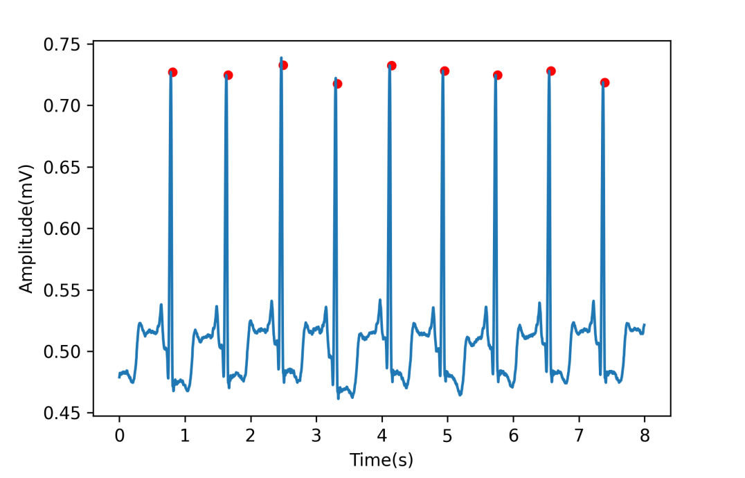
All ECG data were downsampled to 250Hz. A low-pass Butterworth filter with a cut-off frequency of 50 Hz was applied on AFDB, CHDB and VFDB to eliminate the ECG baseline wander. The ECG signals were further rescaled to values between 0 and 1 by applying a min-max scaling to reduce inter-dataset discrepancy, caused by the usage of different sensor hardware for ECG signal measurement. Both the AF datasets provide R-peak values. However, during deployment, there will be no clinical expert intervention to mark the R-peak values and the pipeline will receive only ECG data. Hence, R-peaks were automatically extracted for both experimentation and deployment.
The ECG data from both AFDB and CHDB were segmented with a window length of 5 seconds and an overlap of 1 second. The datasets provide fibrillations as well as flutters and junctional rhythms in their annotations. Each window has 5 seconds of AF annotations and the decision to label an entire window as a positive class depends on a threshold parameter . If the ratio of the number of AF annotations and the total number of annotations (AF and non-AF) exceeds the threshold , then the window segment is classified as an AF signal. The chosen value of in this study is as adapted from Hongpo Zhang et al. [18].
V Pipeline Architecture
The pipeline is an end-to-end workflow that takes raw ECG as input and delivers AF prediction. The raw ECG input is passed to a data pre-processing and feature extraction engine which transforms the signal and extracts the necessary features for AF detection. This engine is pipelined to a scalable ML classifier that outputs the prediction. The architecture of this pipeline is shown in Fig. V. The sequential stages of the pipeline are described in-depth in the following subsections.
V-A Feature Extraction Engine
The Feature Extraction Engine of the pipeline contains 4 sequential stages, namely Baseline Wander Removal , Scaling , R-peak Detection and Feature Extraction which are explained in detail in Section IV. is the set of raw ECG values with being window length in seconds, the sampling frequency in Hz, the Heart Rate Variability (HRV) features, and the variable subset of features discussed in detail, in Section VI. is depicted in Equation 1.
| (1) |
| (2) |
For this study, HRV features were considered, primarily owing to their superior relevance when compared to general non-linear features such as Shannon Entropy, Renyi Entropy and Tsallis entropy [20]. As stated by Gokul H et al. [21], frequency domain features involve Fast Fourier Transformations which are inherently dilatory to extract. Being statistical in nature, time-domain features can be extracted with less to no delay. converts R-peaks to 14 time-domain features, as shown in Table I.
V-B Resource-efficient Classifier
The algorithm used, Bonsai [22], is a tree learner specifically designed for severely resource-constrained devices. Bonsai learns a sparse project matrix that projects the input vector to a lower dimension to reduce data usage. This is implemented in a streaming fashion so as to even accommodate devices with RAMs small enough to not be able to fit a single vector.
Bonsai learns a single, shallow, sparse tree that uses enhanced nodes — both internal and leaf nodes make non-linear predictions. The overall prediction for a point is the sum of the individual node predictions along the path traversed by the point. Path-based prediction allows Bonsai to accurately learn non-linear decision boundaries while sharing parameters along paths to further reduce model size.
Rather than learning the tree node by node in a greedy fashion, all nodes are learned jointly, along with the sparse projection matrix, so as to optimally allocate memory budgets to each node while maximizing prediction accuracy.
VI Feature Selection and Training
VI-A Feature Importance
As the prediction time of the classifier is directly proportional to the number of features used, feature selection was carried out with the aim of finding out the optimal set of features such that the performance of the underlying classifier was maximized while minimizing the number of features selected. This resulted in an optimal feature subset which reduced the computational cost of the classifier and the processing time of .
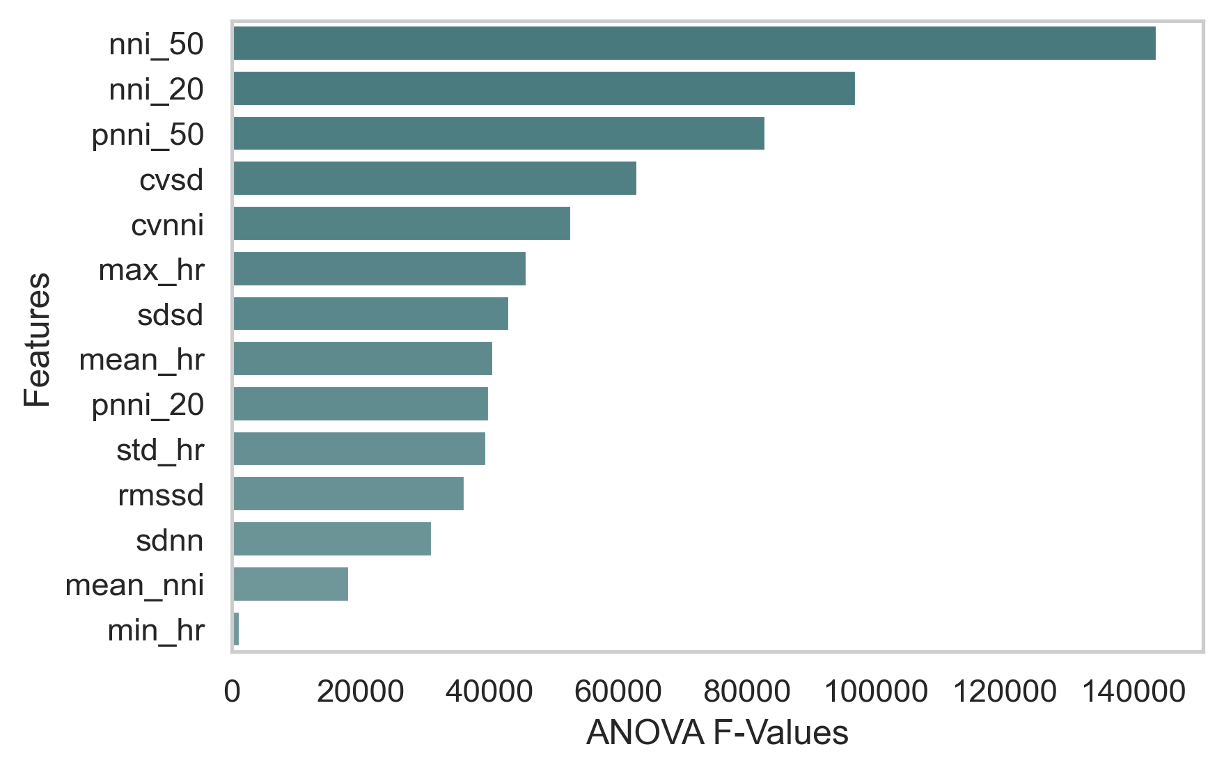
Analysis of Variance (ANOVA) [23] F-test was carried out between each of the independent variables and the predictor variable. An F-statistic or F-value is a measure that determines if the variance between the means of the two populations are significantly different. The higher the value of F-statistic, the higher is the predictive power. The F-values of the extracted features from both the datasets are computed and shown in Fig. 2 and 3. The features are arranged in descending order of their F-values indicating their feature importance in as shown Equation 3.
| (3) | ||||
VI-B Training
A considerable number of AI systems in the healthcare domain fall short of achieving generalizability, thus clinical applicability. Generalization can be hard due to technical differences between sites (including differences in equipment) as well as variations in local clinical and administrative practices [24]. In order to validate the generalizability, we used 2 datasets that collected data under different clinical settings. We constructed a robust train-test strategy where the models were trained and tested on different datasets. The models were also tested on the same dataset it was trained on to establish a point of comparison. This train-test strategy is elucidated in Tab. II.
| (4) |
| (5) |
Models were trained on several subsets of features to choose the optimal subset based on performance, memory requirements and pipeline inference time. In and , the classifier was trained on feature subsets , the most important features chosen using ANOVA as discussed in Section VI-A. The best feature subsets for and were obtained based on accuracy. and were trained on two subset of features each, as derived from and . A 5-fold cross validation was implemented for and . The trained models were deployed onto a Raspberry Pi 3 Model B and the results are discussed in the Section VII.
| Training | |||||||||
|---|---|---|---|---|---|---|---|---|---|
| AFDB(A) | CHDB(C) | ||||||||
| Testing | AFDB (A) |
|
|
||||||
| CHDB(C) |
|
|
|||||||

VII Results and Analysis
All the observations were carried out on a Raspberry Pi 3 Model B and the results were recorded.
VII-A Metrics
The metrics extensively found in literature and throughout this paper are given below by the formulae,
| (6) |
| (7) |

| Model | Data | Accuracy | Precision | Recall | F1 Score | Model Size (in kB) | |||
| Class 0 | Class 1 | Class 0 | Class 1 | Class 0 | Class 1 | ||||
| Decision Tree | CHDB | 93% | 0.96 | 0.90 | 0.89 | 0.96 | 0.93 | 0.93 | 378 |
| AFDB | 88% | 0.89 | 0.88 | 0.87 | 0.90 | 0.88 | 0.89 | 348 | |
| Random Forest | CHDB | 83% | 0.82 | 0.85 | 0.86 | 0.81 | 0.84 | 0.83 | 30699 |
| AFDB | 87% | 0.88 | 0.87 | 0.86 | 0.88 | 0.87 | 0.87 | 29388 | |
| Support Vector Classifier | CHDB | 83% | 0.82 | 0.83 | 0.84 | 0.82 | 0.83 | 0.83 | 563 |
| AFDB | 89% | 0.88 | 0.89 | 0.90 | 0.88 | 0.89 | 0.89 | 604 | |
| Extra Trees Classifier | CHDB | 95% | 0.97 | 0.93 | 0.93 | 0.97 | 0.95 | 0.95 | 91811 |
| AFDB | 92% | 0.95 | 0.89 | 0.88 | 0.95 | 0.91 | 0.92 | 91289 | |
| (8) |
| (9) |
= events classified as events
= - events classified as events
= - events classified as - events
= events classified as - events
The other measurements used to quantify our model’s performance on the embedded device include model size and inference time. Model size is the memory footprint of the classifier on the embedded device. Inference time is termed as the total processing time of .
VII-B Bonsai Results and Analysis
The most optimal feature subset can be either chosen solely with respect to the model performance or based on the compromise between model performance and size. The reasons for choosing a feature subset for both cases are as follows:
VII-B1 Best model performance
We discerned the best scores for with respect to accuracy, sensitivity and specificity was 91.7%, 95.1% and 88.1% was when used, respectively. Similarly, for , Bonsai delivers the best performance using with values of 92.3%, 92.7% and 91.8%, respectively. For and , we observe that gives the best accuracy (90.3%, 89.8%) compared to . Since uses fewer features than it has lower inference time and model size. Hence, we conclude that is the most optimal feature subset if performance is given the most importance.
VII-B2 Best trade-off between model size and performance
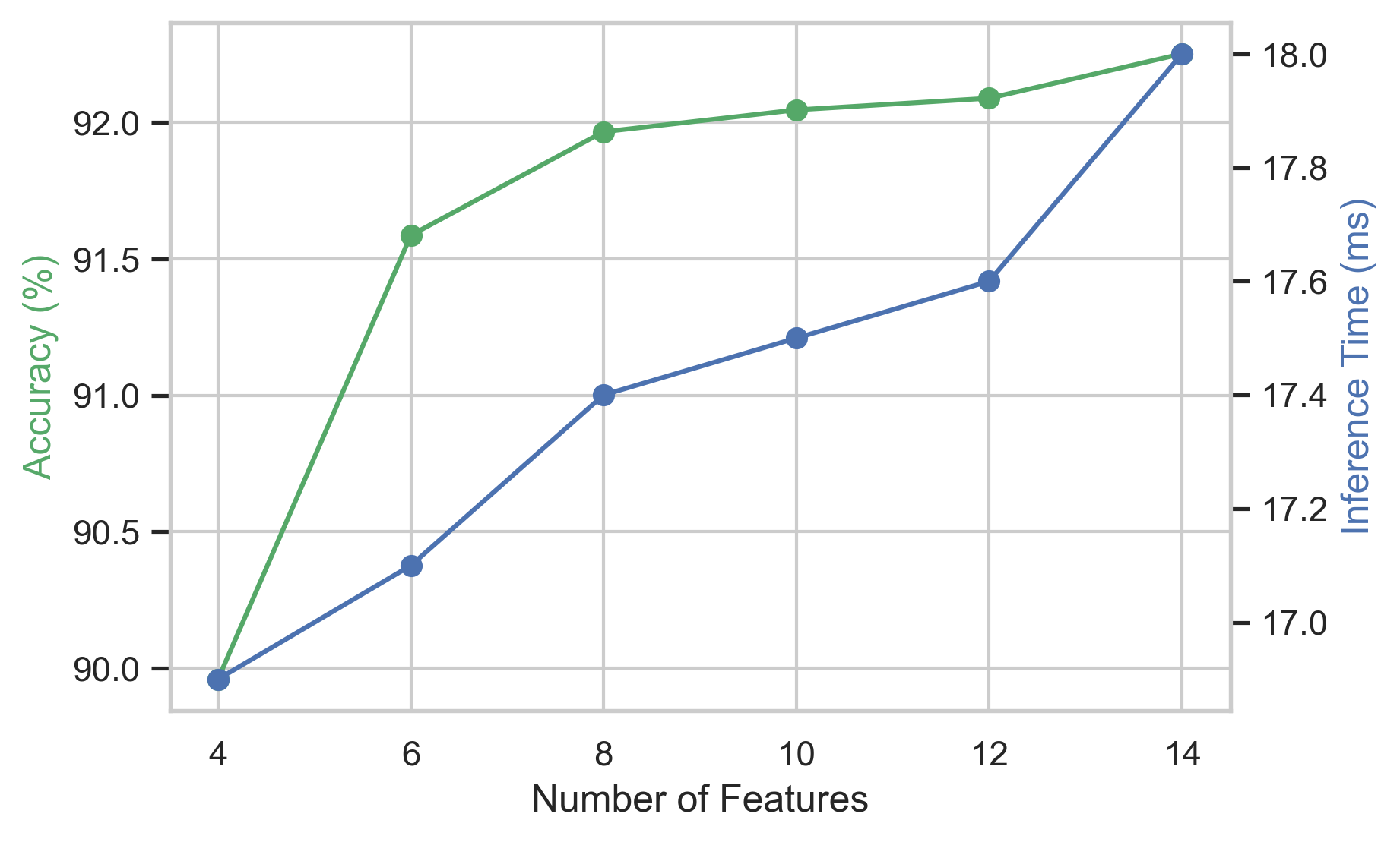
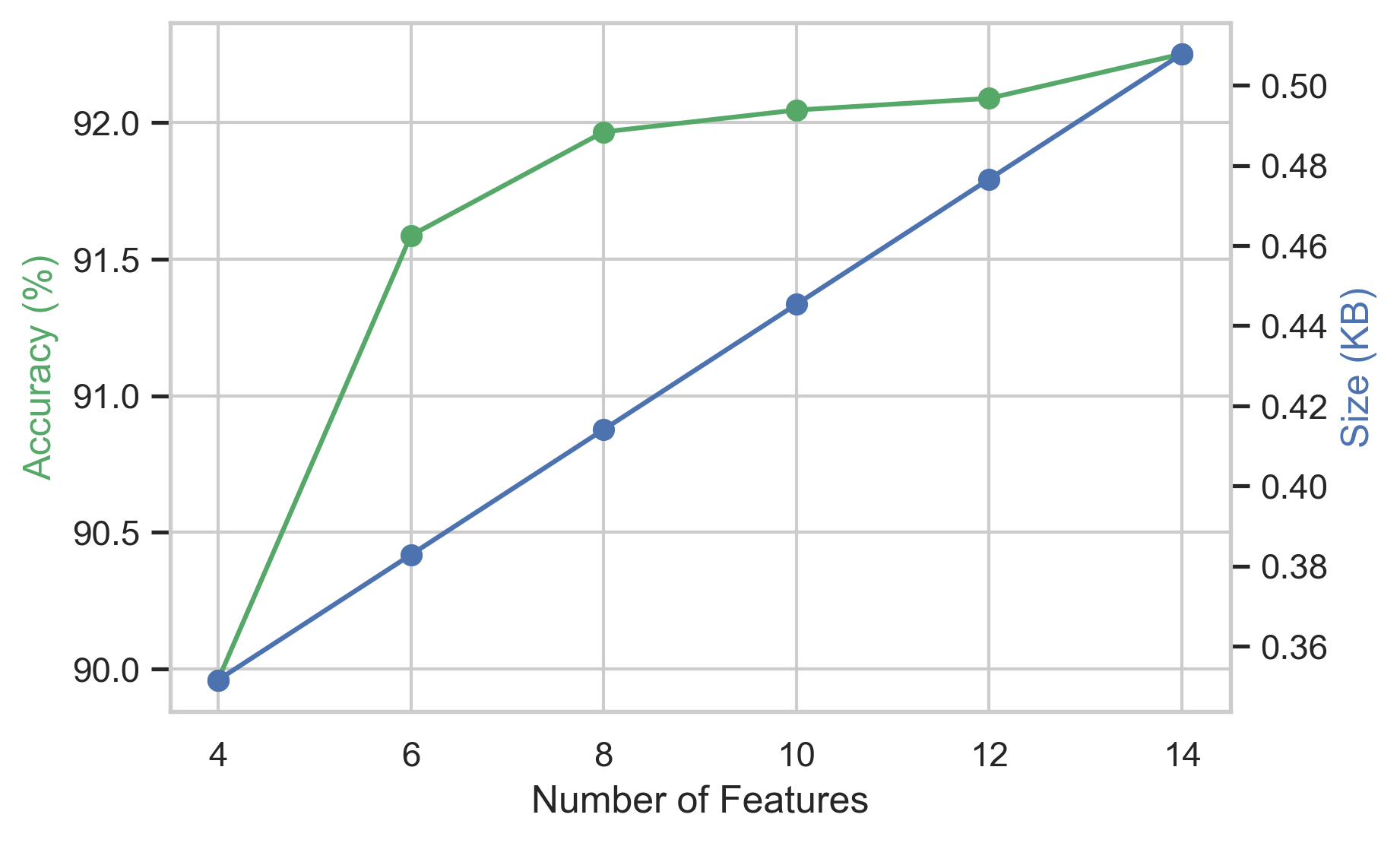
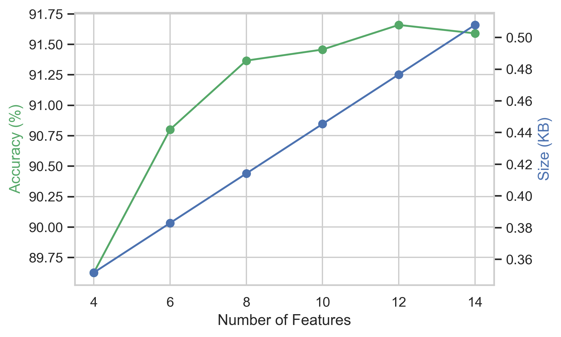
As seen in the below plots, there is a general trend of increase in accuracy with the increase in the number of features. But the increase in accuracy slows down after the top 8 features for both datasets despite a linear increase in model size as seen in Fig. 7 and 9. If the optimal feature subset were to be chosen based on the compromise between model performance and size, or would be chosen. Considering CHDB, when the number of features used was increased from 4 () to 8 () the accuracy increased by 2.0% while the model size increases by 0.062 KB, but when the number of features used was increased from 8 () to 14 () the accuracy increased only by 0.3% while the model size increases by 0.094 KB, the same trend is seen in AFDB.
| CNN + GRU | Bonsai | |
|---|---|---|
| ECG window | 1 256 | 1 1250 |
| Memory [KB] | 210.00 | 0.508 |
| Accuracy [%] | 86.1 | 92.3 |
| Inference [ms] | 94.8 | 16.9 |
We observe regardless of an increase in the number of features, Bonsai’s inference time remained unchanged. Additionally, when compared to the previous SoA embedded implementation [13], our classifier’s accuracy was 6.2% higher, 413 compact in terms of model size and 5.2 faster in terms of inference time (Table IV).
VII-C Standard ML models
To gauge the performance of our classifier, standard ML models such as Decision Trees, Random Forests, Extra Trees and Support Vector Classifier (SVC) were considered as a baseline for comparison. Since Bonsai is a tree-based classifier, three tree-based standard ML models were chosen for a fair comparison. These classifiers were trained on the most optimal feature subset , as derived in Section VII-B1. The classification scores and the memory footprint of these models were reported in Table III. Bonsai was able to outperform the best performing ML model (Extra Trees) around in terms of memory footprint with a mere trade-off of 2% classification accuracy. Bonsai also surpassed the most compact ML model (Decision trees) by a factor of 685.
| Data | Feature Subsets | Accuracy (%) | Precision (%) | Recall (%) | F1 Score (%) | Model Size |
|
|
|||||||
|---|---|---|---|---|---|---|---|---|---|---|---|---|---|---|---|
| (KB) | Time (ms) | Time (ms) | |||||||||||||
| Class 0 | Class 1 | Class 0 | Class 1 | Class 0 | Class 1 | ||||||||||
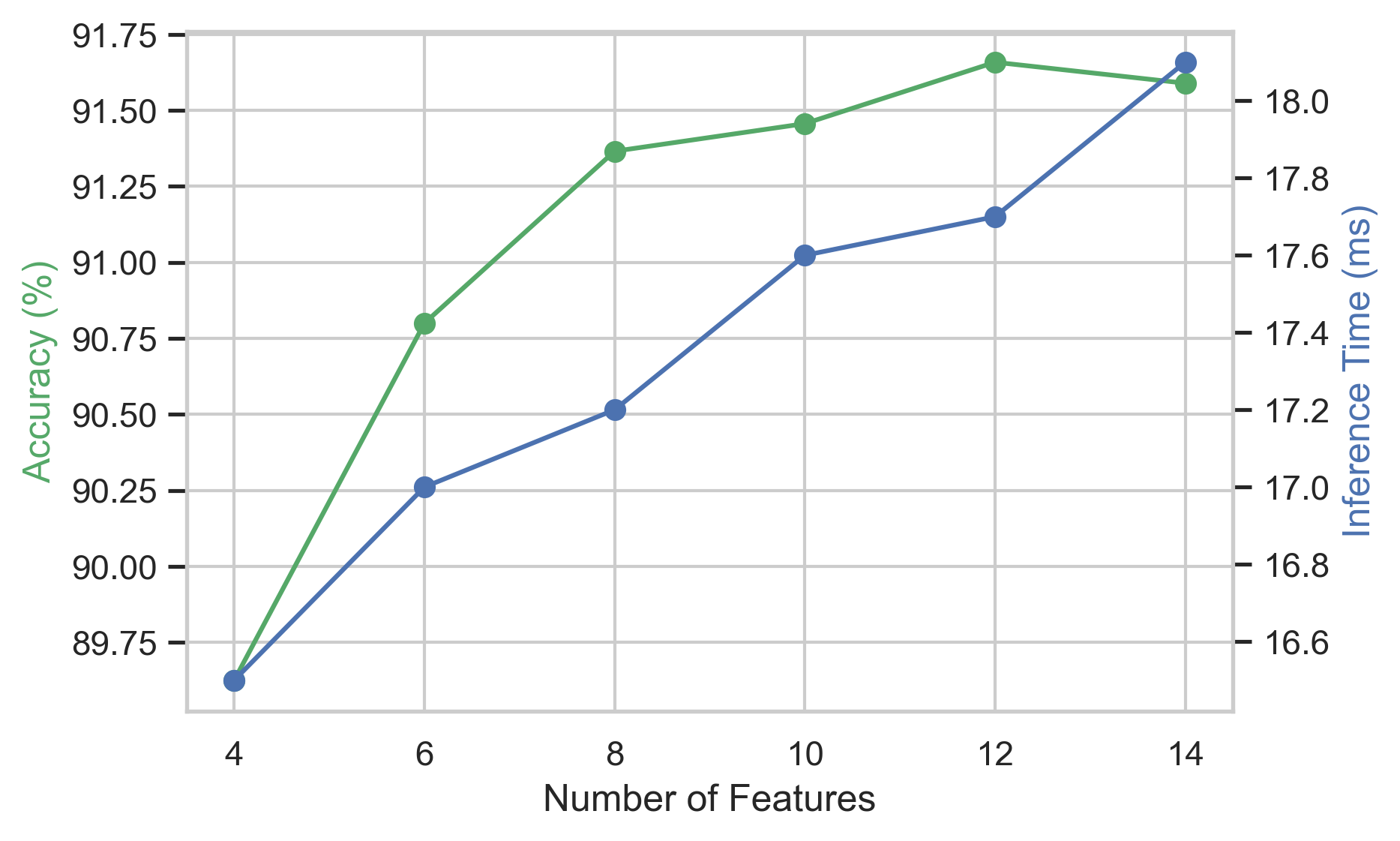
| 89.60 | 94.16 | 85.95 | 84.50 | 94.75 | 89.06 | 90.13 | 0.352 | 3.7 | 16.5 | ||||||
| 90.80 | 95.20 | 87.18 | 85.93 | 95.67 | 90.32 | 91.22 | 0.383 | 3.7 | 17.0 | ||||||
| 91.40 | 94.72 | 88.51 | 87.62 | 95.10 | 91.02 | 91.68 | 0.414 | 3.7 | 17.2 | ||||||
| 91.50 | 94.97 | 88.47 | 87.55 | 95.36 | 91.10 | 91.78 | 0.445 | 3.7 | 17.6 | ||||||
| 91.70 | 94.88 | 88.89 | 88.07 | 95.24 | 91.34 | 91.95 | 0.477 | 3.7 | 17.7 | ||||||
| 91.60 | 94.73 | 88.85 | 88.05 | 95.12 | 91.27 | 91.87 | 0.508 | 3.7 | 18.1 | ||||||
| 89.95 | 91.34 | 88.69 | 88.31 | 91.62 | 89.79 | 90.12 | 0.352 | 3.7 | 16.9 | ||||||
| 91.60 | 92.18 | 91.03 | 90.90 | 92.28 | 91.53 | 91.64 | 0.383 | 3.7 | 16.9 | ||||||
| 91.97 | 92.54 | 91.42 | 91.30 | 92.63 | 91.91 | 92.02 | 0.414 | 3.7 | 17.4 | ||||||
| 92.05 | 92.03 | 92.06 | 92.08 | 92.03 | 92.05 | 92.04 | 0.445 | 3.7 | 17.5 | ||||||
| 92.09 | 92.31 | 91.88 | 91.83 | 92.34 | 92.07 | 92.11 | 0.477 | 3.7 | 17.6 | ||||||
| 92.25 | 92.64 | 91.87 | 91.79 | 92.71 | 92.21 | 92.29 | 0.508 | 3.7 | 18.0 | ||||||
| 90.30 | 88.90 | 90.50 | 90.70 | 88.70 | 89.80 | 89.60 | 0.477 | 3.7 | 16.3 | ||||||
| 89.70 | 89.90 | 88.60 | 88.40 | 90.10 | 89.10 | 89.30 | 0.508 | 3.7 | 16.4 | ||||||
| 89.80 | 95.20 | 85.50 | 83.80 | 95.80 | 89.10 | 90.30 | 0.477 | 3.7 | 16.6 | ||||||
| 89.60 | 95.80 | 84.90 | 82.80 | 96.30 | 88.80 | 90.20 | 0.508 | 3.7 | 16.9 | ||||||
VII-D Pipeline Analysis
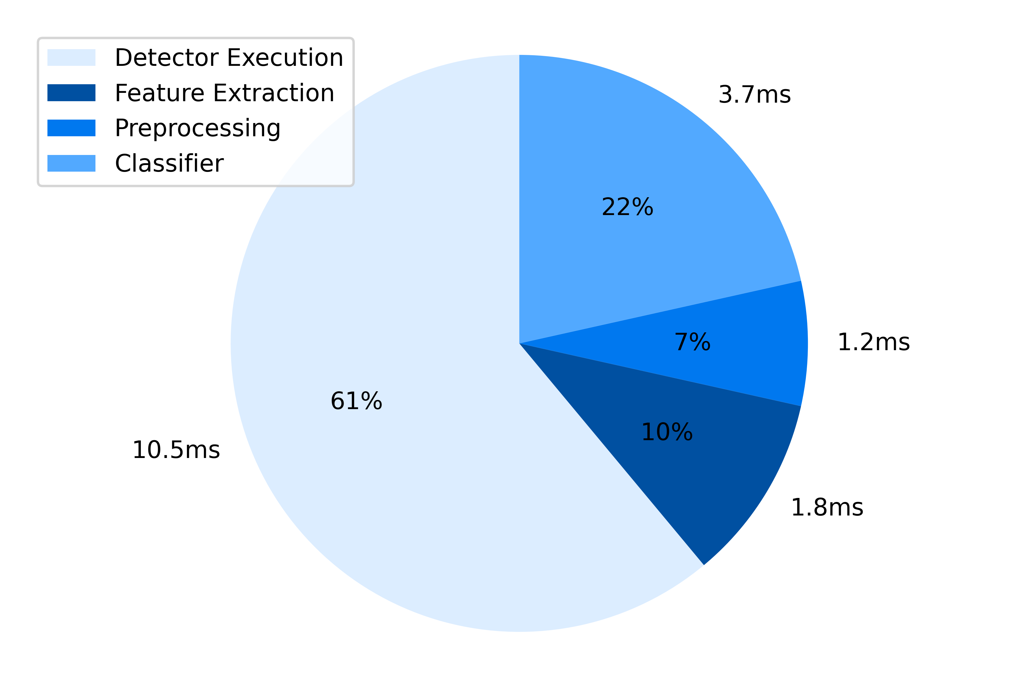
As inferred from the Fig. 5, pipeline inference time is largely occupied (61%) by R-peak detector execution time. It is observed from Fig. 6 and 8 that pipeline inference time increases with growth in the number of features, however, that increase is insignificant (3%-10%).
In order to prove the versatility of our pipeline for the detection of other arrhythmias, the pipeline was trained and tested on Ventricular Fibrillation Database as well. The results of which are accuracy - 89%, F1 score - 86%, precision - 80% and recall - 93%. These scores validate that the proposed pipeline performs well for arrhythmia detection in general.
VIII Conclusion
In this research, we present a novel clinically viable end-to-end pipeline for AF detection. The proposed work outperforms the present SoA embedded implementation with respect to the accuracy, inference time and memory footprint. On average, there was a 6% absolute increase in overall accuracy, while the inference times were observed to be 5.2 lesser and the model size was 403 times smaller when compared to the state-of-the-art model.
The pipeline thus facilitates accurate AF detection, with a significant reduction in latency and memory footprint. Hence they can be pushed onto ultra-edge devices to make real-time on-device predictions. In the future, our end-to-end pipeline could eventually be integrated into a wearable device that acquires and processes ECG signals for arrhythmia detection in real-time.
References
- [1] Anne M. Gillis “Clinical Trials of Pacing for Maintenance of Sinus Rhythm” In Journal of Interventional Cardiac Electrophysiology 10.1, 2004, pp. 55–62 DOI: 10.1023/B:JICE.0000011346.32325.b3
- [2] Yoko Miyasaka et al. “Secular Trends in Incidence of Atrial Fibrillation in Olmsted County, Minnesota, 1980 to 2000, and Implications on the Projections for Future Prevalence” In Circulation 114.2, 2006, pp. 119–125 DOI: 10.1161/CIRCULATIONAHA.105.595140
- [3] M. Shoemaker and Dan M. Roden “Atrial Fibrillation Is a Complex Trait” In Circulation Research 127.2, 2020, pp. 244–246 DOI: 10.1161/CIRCRESAHA.120.317112
- [4] Stewart S, Hart CL, Hole DJ and McMurray JJ. “A population-based study of the long-term risks associated with atrial fibrillation: 20-year follow-up of the Renfrew/Paisley study” In 2002 Oct 1;113(5):359-64. doi: 10. 1016/s0002-9343(02) 01236-6. PMID: 12401529, 2002
- [5] Christopher X. Wong, Dennis H. Lau and Prashanthan Sanders “Atrial Fibrillation Epidemic and Hospitalizations” In Circulation 129.23, 2014, pp. 2361–2363 DOI: 10.1161/CIRCULATIONAHA.114.010073
- [6] Leif Friberg et al. “High Prevalence of Atrial Fibrillation Among Patients With Ischemic Stroke” In Stroke 45.9, 2014, pp. 2599–2605 DOI: 10.1161/STROKEAHA.114.006070
- [7] Sumeet S. Chugh et al. “Worldwide Epidemiology of Atrial Fibrillation” In Circulation 129.8, 2014, pp. 837–847 DOI: 10.1161/CIRCULATIONAHA.113.005119
- [8] Yanrui Jin, Chengjin Qin, Jianfeng Tao and Chengliang Liu “An accurate and adaptative cutterhead torque prediction method for shield tunneling machines via adaptative residual long-short term memory network” In Mechanical Systems and Signal Processing 165, 2022, pp. 108312 DOI: https://doi.org/10.1016/j.ymssp.2021.108312
- [9] Jibin Wang “Automated Detection of Atrial Fibrillation and Atrial Flutter in ECG Signals Based on Convolutional and Improved Elman Neural Network” In Know.-Based Syst. 193.C NLD: Elsevier Science Publishers B. V., 2020 DOI: 10.1016/j.knosys.2019.105446
- [10] Sajad Mousavi, Fatemeh Afghah, Abolfazl Razi and U. Acharya “ECGNET: Learning where to attend for detection of atrial fibrillation with deep visual attention”, 2019 arXiv:1812.07422 [q-bio.QM]
- [11] Nurul Hossain et al. “A Low-cost, Low-energy Wearable ECG System with Cloud-Based Arrhythmia Detection”, 2020 DOI: 10.1109/TENSYMP50017.2020.9230619
- [12] Samuel A. Setiawan, Aulia A. Iskandar and Muhammad Fathony “Development of Cloud Computing Algorithm for Arrhythmia Detection” In 2020 FORTEI-International Conference on Electrical Engineering (FORTEI-ICEE), 2020, pp. 53–58 DOI: 10.1109/FORTEI-ICEE50915.2020.9249808
- [13] Antonino Faraone and Ricard Delgado-Gonzalo “Convolutional-Recurrent Neural Networks on Low-Power Wearable Platforms for Cardiac Arrhythmia Detection” In 2020 2nd IEEE International Conference on Artificial Intelligence Circuits and Systems (AICAS), 2020, pp. 153–157 DOI: 10.1109/AICAS48895.2020.9073950
- [14] George Moody and Roger Mark “MIT-BIH atrial fibrillation Database” In MIT-BIH Atrial Fibrillation Database v1.0.0, 2000 URL: https://physionet.org/content/afdb/1.0.0/
- [15] Gari Clifford et al. “Af classification from a short single lead ecg recording - the physionet computing in cardiology challenge 2017” In AF Classification from a Short Single Lead ECG Recording - The PhysioNet Computing in Cardiology Challenge 2017 v1.0.0, 2017 URL: https://physionet.org/content/challenge-2017/1.0.0/
- [16] “MIT-BIH malignant Ventricular Ectopy database” In MIT-BIH Malignant Ventricular Ectopy Database v1.0.0, 1999 URL: https://physionet.org/content/vfdb/1.0.0/
- [17] Goldberger AL, Glass machine L and Amaral LAN “Physionet” In PhysioNet URL: https://physionet.org/
- [18] Hongpo Zhang et al. “SS-SWT and SI-CNN: An Atrial Fibrillation Detection Framework for Time-Frequency ECG Signal” In Journal of Healthcare Engineering 2020, 2020, pp. 1–11 DOI: 10.1155/2020/7526825
- [19] G.. Nason and B.. Silverman “The Stationary Wavelet Transform and some Statistical Applications” In Wavelets and Statistics New York, NY: Springer New York, 1995, pp. 281–299 DOI: 10.1007/978-1-4612-2544-7˙17
- [20] Task Force European Society of Cardiology the North American Society of Pacing Electrophysiology “Heart Rate Variability” In Circulation 93.5, 1996, pp. 1043–1065 DOI: 10.1161/01.CIR.93.5.1043
- [21] Gokul H. et al. “Gait Recovery System for Parkinson’s Disease using Machine Learning on Embedded Platforms”, 2020 arXiv:2004.05811 [eess.SP]
- [22] Ashish Kumar, Saurabh Goyal and Manik Varma “Resource-Efficient Machine Learning in 2 KB RAM for the Internet of Things” In Proceedings of the 34th International Conference on Machine Learning - Volume 70, ICML’17 Sydney, NSW, Australia: JMLR.org, 2017, pp. 1935–1944
- [23] Ellen R Girden “ANOVA: Repeated measures” Sage, 1992
- [24] C.. Kelly, A. Karthikesalingam and M. Suleyman “Key challenges for delivering clinical impact with artificial intelligence” In BMC Med 17 195, 2019
- [25] Mark Lown et al. “Machine learning detection of Atrial Fibrillation using wearable technology” In PLOS ONE 15.1 Public Library of Science, 2020, pp. 1–9 DOI: 10.1371/journal.pone.0227401
- [26] Dennis, Don Kurian and Gaurkar, Yash and Gopinath, Sridhar and Goyal, Sachin and Gupta, Chirag and Jain, Moksh and Jaiswal, Shikhar and Kumar, Ashish and Kusupati, Aditya and Lovett, Chris and Patil, Shishir G and Saha, Oindrila and Simhadri, Harsha Vardhan “EdgeML: Machine Learning for resource-constrained edge devices” URL: https://github.com/Microsoft/EdgeML
- [27] Supreeth Prajwal Shashikumar et al. “A deep learning approach to monitoring and detecting atrial fibrillation using wearable technology” In 2017 IEEE EMBS International Conference on Biomedical Health Informatics (BHI), 2017, pp. 141–144 DOI: 10.1109/BHI.2017.7897225
- [28] Abhijith Ragav et al. “Scalable Deep Learning for Stress and Affect Detection on Resource-Constrained Devices” In 2019 18th IEEE International Conference On Machine Learning And Applications (ICMLA), 2019, pp. 1585–1592 DOI: 10.1109/ICMLA.2019.00261