longtable
Trimmed Harrell-Davis quantile estimator based on the highest density interval of the given width
Abstract
Traditional quantile estimators that are based on one or two order statistics are a common way to estimate distribution quantiles based on the given samples. These estimators are robust, but their statistical efficiency is not always good enough. A more efficient alternative is the Harrell-Davis quantile estimator which uses a weighted sum of all order statistics. Whereas this approach provides more accurate estimations for the light-tailed distributions, it’s not robust. To be able to customize the trade-off between statistical efficiency and robustness, we could consider a trimmed modification of the Harrell-Davis quantile estimator. In this approach, we discard order statistics with low weights according to the highest density interval of the beta distribution.
Keywords: quantile estimation, robust statistics, Harrell-Davis quantile estimator.
600mm(.5)
This is an original manuscript of an article published by Taylor & Francis
in Communications in Statistics — Simulation and Computation on 17 March 2022,
available online: https://www.tandfonline.com/10.1080/03610918.2022.2050396
Introduction
We consider a problem of quantile estimation for the given sample. Let be a sample with elements: . We assume that all sample elements are sorted () so that we could treat the element as the order statistic . Based on the given sample, we want to build an estimation of the quantile .
The traditional way to do this is to use a single order statistic or a linear combination of two subsequent order statistics. This approach could be implemented in various ways. A classification of the most popular implementations could be found in [HF96]. In this paper, Rob J. Hyndman and Yanan Fan describe nine types of traditional quantile estimators which are used in statistical computer packages. The most popular approach in this taxonomy is Type 7 which is used by default in R, Julia, NumPy, and Excel:
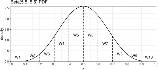
Traditional quantile estimators have simple implementations and a good robustness level. However, their statistical efficiency is not always good enough: the obtained estimations could noticeably differ from the true distribution quantile values. The gap between the estimated and true values could be decreased by increasing the number of used order statistics. In [HD82], Frank E. Harrell and C. E. Davis suggest estimating quantiles using a weighted sum of all order statistics:
where is the regularized incomplete beta function, , . To get a better understanding of this approach, we could look at the probability density function of the beta distribution (see Figure 1). If we split the interval into segments of equal width, we can define as the area under curve in the segment. Since is the cumulative distribution function of , we can express as .
The Harrell-Davis quantile estimator is suggested in [DN03], [GK12], [Wil16], and [GC20] as an efficient alternative to the traditional estimators. In [YSD85], asymptotic equivalence for the traditional sample median and the Harrell–Davis median estimator is shown.
The Harrell-Davis quantile estimator shows decent statistical efficiency in the case of light-tailed distributions: its estimations are much more accurate than estimations of the traditional quantile estimators. However, the improved efficiency has a price: is not robust. Since the estimation is a weighted sum of all order statistics with positive weights, a single corrupted element may spoil all the quantile estimations, including the median. It may become a severe drawback in the case of heavy-tailed distributions in which it’s a typical situation when we have a few extremely large outliers. In such cases, we use the median instead of the mean as a measure of central tendency because of its robustness. Indeed, if we estimate the median using the traditional quantile estimators like , its asymptotic breakdown point is 0.5. Unfortunately, if we switch to , the breakdown point becomes zero so that we completely lose the median robustness.
Another severe drawback of is its computational complexity. If we have a sorted array of numbers, a traditional quantile estimation could be computed using simple operations. For an unsorted sample, there are approaches that allow getting an order statistic using operations (e.g., see [Ale17]). If we estimate the quantiles using , we need operations for a sorted array. Moreover, these operations involve computation of values which are pretty expensive from the computational point of view.
Alternatively, we could consider the Sfakianakis-Verginis quantile estimator (see [SV08]) or the Navruz-Özdemir quantile estimator (see [NÖ20]) which are also based on a weighted sum of all order statistics. However, they also have the disadvantages listed above.
Neither nor fit all kinds of problem. is simple, robust, and computationally fast, but its statistical efficiency doesn’t always satisfy the business requirements. could provide better statistical efficiency, but it’s computationally slow and not robust.
To get a reasonable trade-off between and , we consider a trimmed modification of the Harrell-Davis quantile estimator. The core idea is simple: we take the classic Harrell-Davis quantile estimator, find the highest density interval of the underlying beta distribution, discard all the order statistics outside the interval, and calculate a weighted sum of the order statistics within the interval. The obtained quantile estimation is more robust than (because it doesn’t use extreme values) and typically more statistically efficient than (because it uses more than only two order statistics). Let’s discuss this approach in detail.
The trimmed Harrell-Davis quantile estimator
The estimators based on one or two order statistics are not efficient enough because they use too few sample elements. The estimators based on all order statistics are not robust enough because they use too many sample elements. It looks reasonable to consider a quantile estimator based on a variable number of order statistics. This number should be large enough to ensure decent statistical efficiency but not too large to exclude possible extreme outliers.
A robust alternative to the mean is the trimmed mean. The idea behind it is simple: we should discard some sample elements at both ends and use only the middle order statistics. With this approach, we can customize the trade-off between robustness and statistical efficiency by controlling the number of the discarded elements. If we apply the same idea to , we can build a trimmed modification of the Harrell-Davis quantile estimator. Let’s denote it as .
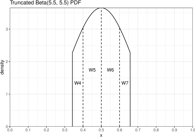
In the case of the trimmed mean, we typically discard the same number of elements on each side. We can’t do the same for because the array of order statistic weights is asymmetric. It looks reasonable to drop the elements with the lowest weights and keep the elements with the highest weights. Since the weights are assigned according to the beta distribution, the range of order statistics with the highest weight concentration could be found using the beta distribution highest density interval. Thus, once we fix the proportion of dropped/kept elements, we should find the highest density interval of the given width. Let’s denote the interval as where . The order statistics weights for should be defined using a part of the beta distribution within this interval. It gives us the truncated beta distribution (see Figure 2).
We know the CDF for which is used in : . For , we need the CDF for which could be easily found:
The final equation has the same form as :
There is only one thing left to do: we should choose an appropriate width of the beta distribution highest density interval. In practical application, this value should be chosen based on the given problem: researchers should carefully analyze business requirements, describe desired robustness level via setting the breakdown point, and come up with a value that satisfies the initial requirements.
However, if we have absolutely no information about the problem, the underlying distribution, and the robustness requirements, we can use the following rule of thumb which gives the starting point: . We denote with such a value as . In most cases, it gives an acceptable trade-off between the statistical efficiency and the robustness level. Also, has a practically reasonable computational complexity: instead of for . For example, if , we have to process only 100 sample elements and calculate 101 values of .
An example Let’s say we have the following sample:
Nine elements were randomly taken from the standard normal distribution . The last element is an outlier. The weight coefficient for an are presented in Table LABEL:tab:t1.
| () | |||
|---|---|---|---|
| () | |||
| 1 | -0.565 | 0.0005 | 0 |
| 2 | -0.106 | 0.0146 | 0 |
| 3 | -0.095 | 0.0727 | 0 |
| 4 | 0.363 | 0.1684 | 0.1554 |
| 5 | 0.404 | 0.2438 | 0.3446 |
| 6 | 0.633 | 0.2438 | 0.3446 |
| 7 | 1.371 | 0.1684 | 0.1554 |
| 8 | 1.512 | 0.0727 | 0 |
| 9 | 2.018 | 0.0146 | 0 |
| 10 | 0.0005 | 0 | |
| () |
Here are the corresponding quantile estimations:
As we can see, is heavily affected by the outlier . Meanwhile, gives a reasonable median estimation because it uses a weighted sum of four middle order statistics.
Beta distribution highest density interval of the given width
In order to build the truncated beta distribution for , we have to find the highest density interval of the required width . Thus, for the given , we should provide an interval :
Let’s briefly discuss how to do this. First of all, we should calculate the mode of (non-degenarate cases are presented in Figure 3):
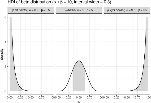
The actual value of depends on the specific case from the above list which defines the mode location. Three of these cases are easy to handle:
-
•
Degenerate case : There is only one way to get such a situation: . Since such a sample contains a single element, it doesn’t matter how we choose the interval.
-
•
Left border case : The mode equals zero, so the interval should be “attached to the left border”: .
-
•
Right border case : The mode equals one, so the interval should be “attached to the right border”:
The fourth case is the middle case (), the HDI should be inside . Since the density function of the beta distribution is a unimodal function, it consists of two segments: a monotonically increasing segment and a monotonically decreasing segment . The HDI should contain the mode, so
Since , we could also conclude that
Thus,
The density function of the beta distribution is also known (see [CT+21]):
It’s easy to see that for the highest density interval , the following condition is true:
The left border of this interval could be found as a solution of the following equation:
The left side of the equation is monotonically increasing, the right side is monotonically decreasing. The equation has exactly one solution which could be easily found numerically using the binary search algorithm.
Simulation study
Let’s perform a few numerical simulations and see how works in action.111The source code of all simulations is available on GitHub: https://github.com/AndreyAkinshin/paper-thdqe
Simulation 1
Let’s explore the distribution of estimations for , , and . We consider a contaminated normal distribution which is a mixture of two normal distributions: . For our simulation, we use . We generate samples of size 7 randomly taken from the considered distribution. For each sample, we estimate the median using , , and . Thus, we have median estimations for each estimator. Next, we evaluate lower and higher percentiles for each group of estimations. The results are presented in Table LABEL:tab:t2.
| () quantile | HF7 | HD | THD-SQRT |
|---|---|---|---|
| () | |||
| 0.00 | -1.6921648 | -87.6286082 | -1.6041220 |
| 0.01 | -1.1054591 | -9.8771723 | -1.0261234 |
| 0.02 | -0.9832125 | -5.2690083 | -0.9067884 |
| 0.03 | -0.9037046 | -1.7742334 | -0.8298706 |
| 0.04 | -0.8346268 | -0.9921591 | -0.7586603 |
| 0.96 | 0.8172518 | 0.8964743 | 0.7540437 |
| 0.97 | 0.8789283 | 1.1240294 | 0.8052421 |
| 0.98 | 0.9518048 | 4.3675475 | 0.8824462 |
| 0.99 | 1.0806293 | 10.4132583 | 0.9900912 |
| 1.00 | 2.0596785 | 140.5802861 | 1.7060750 |
| () |
We also perform the same experiment using the Fréchet distribution (shape=1) as an example of a right-skewed heavy-tailed distribution. The results are presented in Table LABEL:tab:t3.
| () quantile | HF7 | HD | THD-SQRT |
|---|---|---|---|
| () | |||
| 0.00 | 0.3365648 | 0.4121860 | 0.3720898 |
| 0.01 | 0.5161896 | 0.6684699 | 0.5810966 |
| 0.02 | 0.5703807 | 0.7578653 | 0.6369594 |
| 0.03 | 0.6082605 | 0.8058995 | 0.6834209 |
| 0.04 | 0.6433384 | 0.8460783 | 0.7187727 |
| 0.96 | 4.2510264 | 7.2021571 | 4.6591661 |
| 0.97 | 4.6202217 | 8.3669085 | 5.0186522 |
| 0.98 | 5.2815341 | 10.0274664 | 5.6965864 |
| 0.99 | 6.5037105 | 14.3159366 | 7.1671722 |
| 1.00 | 42.0799646 | 35.3494053 | |
| () |
In Table LABEL:tab:t2, approximately 2% of all results exceed 10 by their absolute values (while the true median value is zero). Meanwhile, the maximum absolute value of the median estimations is approximately . In Table LABEL:tab:t3, the higher percentiles of estimations are also noticeably higher than the corresponding values of .
Thus, is much more resistant to outliers than .
Simulation 2
Let’s compare the statistical efficiency of and . We evaluate the relative efficiency of these estimators against which is a conventional baseline in such experiments. For the quantile, the classic relative efficiency can be calculated as the ratio of the estimator mean squared errors () (see [Dek+05]):
where is the true quantile value. We conduct this simulation according to the following scheme:
-
•
We consider a bunch of different symmetric and asymmetric, light-tailed and heavy-tailed distributions listed in Table LABEL:tab:t4.
-
•
We enumerate all the percentile values from 0.01 to 0.99.
-
•
For each distribution, we generate 200 random samples of the given size. For each sample, we estimate the percentile using , , and . For each estimator, we calculate the arithmetic average of .
-
•
is not a robust metric, so we wouldn’t get reproducible output in such an experiment. To achieve more stable results, we repeat the previous step 101 times and take the median across values for each estimator. This median is our estimation of .
-
•
We evaluate the relative efficiency of and against .
| () Distribution | Support | Skewness | Tailness |
|---|---|---|---|
| () | |||
| Uniform(a=0, b=1) | Symmetric | Light-tailed | |
| Triangular(a=0, b=2, c=1) | Symmetric | Light-tailed | |
| Triangular(a=0, b=2, c=0.2) | Right-skewed | Light-tailed | |
| Beta(a=2, b=4) | Right-skewed | Light-tailed | |
| Beta(a=2, b=10) | Right-skewed | Light-tailed | |
| Normal(m=0, sd=1) | Symmetric | Light-tailed | |
| Weibull(scale=1, shape=2) | Right-skewed | Light-tailed | |
| Student(df=3) | Symmetric | Light-tailed | |
| Gumbel(loc=0, scale=1) | Right-skewed | Light-tailed | |
| Exp(rate=1) | Right-skewed | Light-tailed | |
| Cauchy(x0=0, gamma=1) | Symmetric | Heavy-tailed | |
| Pareto(loc=1, shape=0.5) | Right-skewed | Heavy-tailed | |
| Pareto(loc=1, shape=2) | Right-skewed | Heavy-tailed | |
| LogNormal(mlog=0, sdlog=1) | Right-skewed | Heavy-tailed | |
| LogNormal(mlog=0, sdlog=2) | Right-skewed | Heavy-tailed | |
| LogNormal(mlog=0, sdlog=3) | Right-skewed | Heavy-tailed | |
| Weibull(shape=0.3) | Right-skewed | Heavy-tailed | |
| Weibull(shape=0.5) | Right-skewed | Heavy-tailed | |
| Frechet(shape=1) | Right-skewed | Heavy-tailed | |
| Frechet(shape=3) | Right-skewed | Heavy-tailed | |
| () |
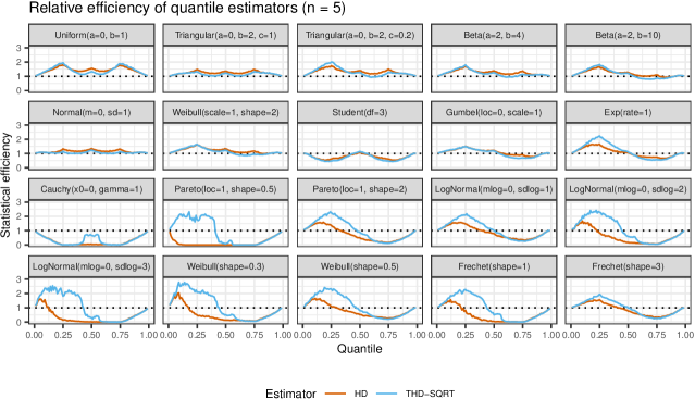
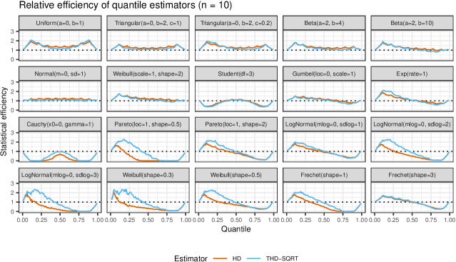
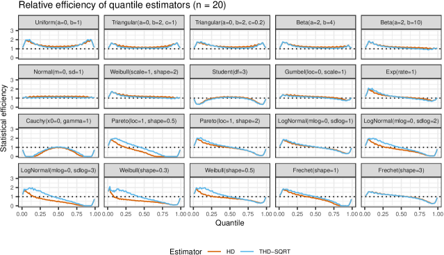
As we can see, is not so efficient as in the case of light-tailed distributions. However, in the case of heavy-tailed distributions, has better efficiency than because the estimations of are corrupted by outliers.
Conclusion
There is no perfect quantile estimator that fits all kinds of problems. The choice of a specific estimator has to be made based on the knowledge of the domain area and the properties of the target distributions. is a good alternative to in the light-tailed distributions because it has higher statistical efficiency. However, if extreme outliers may appear, estimations of could be heavily corrupted. could be used as a reasonable trade-off between and . In most cases, has better efficiency than and it’s also more resistant to outliers than . By customizing the width of the highest density interval, we could set the desired breakdown point according to the research goals. Also, has better computational efficiency than which makes it a faster option in practical applications.
Disclosure statement
The author reports there are no competing interests to declare.
Acknowledgments
The author thanks Ivan Pashchenko for valuable discussions.
Reference implementation
Here is an R implementation of the suggested estimator:
getBetaHdi <- function(a, b, width) {
eps <- 1e-9
if (a < 1 + eps & b < 1 + eps) # Degenerate case
return(c(NA, NA))
if (a < 1 + eps & b > 1) # Left border case
return(c(0, width))
if (a > 1 & b < 1 + eps) # Right border case
return(c(1 - width, 1))
if (width > 1 - eps)
return(c(0, 1))
# Middle case
mode <- (a - 1) / (a + b - 2)
pdf <- function(x) dbeta(x, a, b)
l <- uniroot(
f = function(x) pdf(x) - pdf(x + width),
lower = max(0, mode - width),
upper = min(mode, 1 - width),
tol = 1e-9
)$root
r <- l + width
return(c(l, r))
}
thdquantile <- function(x, probs, width = 1 / sqrt(length(x)))
sapply(probs, function(p) {
n <- length(x)
if (n == 0) return(NA)
if (n == 1) return(x)
x <- sort(x)
a <- (n + 1) * p
b <- (n + 1) * (1 - p)
hdi <- getBetaHdi(a, b, width)
hdiCdf <- pbeta(hdi, a, b)
cdf <- function(xs) {
xs[xs <= hdi[1]] <- hdi[1]
xs[xs >= hdi[2]] <- hdi[2]
(pbeta(xs, a, b) - hdiCdf[1]) / (hdiCdf[2] - hdiCdf[1])
}
iL <- floor(hdi[1] * n)
iR <- ceiling(hdi[2] * n)
cdfs <- cdf(iL:iR/n)
W <- tail(cdfs, -1) - head(cdfs, -1)
sum(x[(iL+1):iR] * W)
})
An implementation of the original Harrell-Davis quantile estimator could be found in the Hmisc package (see [Har21]).
References
- [Ale17] Andrei Alexandrescu “Fast Deterministic Selection” In 16th International Symposium on Experimental Algorithms (SEA 2017) 75, Leibniz International Proceedings in Informatics (LIPIcs) Dagstuhl, Germany: Schloss Dagstuhl–Leibniz-Zentrum fuer Informatik, 2017, pp. 24:1–24:19 DOI: 10.4230/LIPIcs.SEA.2017.24
- [CT+21] Carroll Croarkin and Paul Tobias “NIST/SEMATECH Engineering Statistics Handbook”, 2021 DOI: 10.18434/M32189
- [Dek+05] Frederik Michel Dekking, Cornelis Kraaikamp, Hendrik Paul Lopuhaä and Ludolf Erwin Meester “A Modern Introduction to Probability and Statistics: Understanding why and how”, Springer Texts in Statistics Springer Science & Business Media, 2005
- [DN03] Herbert A David and Haikady N Nagaraja “Order statistics” John Wiley & Sons, 2003 DOI: 10.1002/0471722162
- [GC20] Jean Dickinson Gibbons and Subhabrata Chakraborti “Nonparametric statistical inference” CRC press, 2020
- [GK12] Robert J Grissom and John J Kim “Effect sizes for research: Univariate and multivariate applications” Routledge Academic, 2012 DOI: 10.4324/9781410612915
- [Har21] Frank E Harrell Jr “Hmisc: Harrell Miscellaneous”, 2021 URL: https://CRAN.R-project.org/package=Hmisc
- [HD82] Frank E. Harrell and C.. Davis “A new distribution-free quantile estimator” In Biometrika 69.3 [Oxford University Press, Biometrika Trust], 1982, pp. 635–640 DOI: 10.1093/biomet/69.3.635
- [HF96] Rob J Hyndman and Yanan Fan “Sample quantiles in statistical packages” In The American Statistician 50.4 Taylor & Francis, 1996, pp. 361–365 DOI: 10.2307/2684934
- [NÖ20] Gözde Navruz and A Fırat Özdemir “A new quantile estimator with weights based on a subsampling approach” In British Journal of Mathematical and Statistical Psychology 73.3 Wiley Online Library, 2020, pp. 506–521 DOI: 10.1111/bmsp.12198
- [SV08] Michael E Sfakianakis and Dimitris G Verginis “A new family of nonparametric quantile estimators” In Communications in Statistics—Simulation and Computation® 37.2 Taylor & Francis, 2008, pp. 337–345 DOI: 10.1080/03610910701790491
- [Wil16] Rand R Wilcox “Introduction to robust estimation and hypothesis testing” Academic press, 2016
- [YSD85] Carl N Yoshizawa, Pranab K Sen and C Edward Davis “Asymptotic equivalence of the Harrell-Davis median estimator and the sample median” In Communications in Statistics-Theory and Methods 14.9 Taylor & Francis, 1985, pp. 2129–2136 DOI: 10.1080/03610928508829034