ReGroup: Recursive Neural Networks for Hierarchical Grouping of Vector Graphic Primitives

Abstract.

Selection functionality is as fundamental to vector graphics as it is for raster data. But vector selection is quite different: instead of pixel-level labeling, we make a binary decision to include or exclude each vector primitive. In the absence of intelligible metadata, this becomes a perceptual grouping problem. These have previously relied on heuristics derived from empirical principles like Gestalt Theory, but since these are ill-defined and subjective, they often result in ambiguity. Here we take a data-centric approach to the problem. By exploiting the recursive nature of perceptual grouping, we interpret the task as constructing a hierarchy over the primitives of a vector graphic, which is amenable to learning with recursive neural networks with few human annotations. We verify this by building a dataset of these hierarchies on which we train a hierarchical grouping network. We then demonstrate how this can underpin a prototype selection tool.

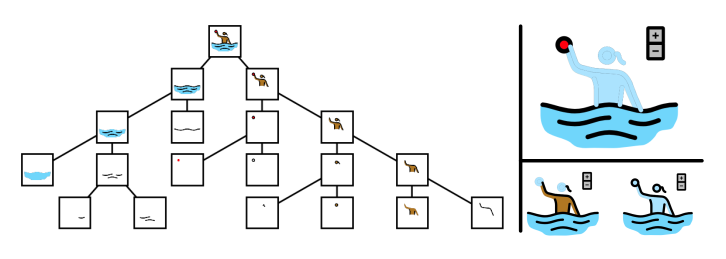
Figure 1. We parse a 2D vector graphics image (root node of the tree on the left) into a perceptually organized hierarchy of graphical elements, and use it to power selection tools. We collect a dataset of such hierarchies and train a neural network that learns to group by recursively merging elements. One of our selection tools (top right) works by selecting an initial path (the swimmer’s face in this example) and using the plus button to traverse to ancestors of the path. The expanded selection is highlighted in light blue. Competing state-of-the-art approaches, Fisher et. al. (Fisher et al., 2021) (inset bottom left) and Suggero (Lindlbauer et al., 2013) (inset bottom right), fail to grow the selection correctly, grouping head and ball in one case and omitting all outlines in the other. This is because handwritten heuristics alone are not robust indicators of grouping affinity: our data-driven method learns to avoid such errors.

1. Introduction

Vector graphics are the de facto standard for wide classes of diagrams, illustrations and other resolution-independent visuals. They are typically expressed as unions of paths: open or closed curves with various geometric and color attributes which constitute atomic elements of the drawings. Editing a semantically meaningful component – such as the head of a human figure or the roof of a house, each of which may comprise several paths – requires that the component first be selected. While careful designers can organize paths into meaningful groups to make selection easier, large quantities of graphics “in the wild” lack much if any such organization, making selection a tedious and finicky process (Lindlbauer et al., 2013; Xu et al., 2012).

Vector editing programs, such as Adobe Illustrator and Inkscape, try to make selecting groups of paths in unorganized graphics easier with tools such as rectangular and lasso selections, in addition to the regular one-click-per-path mode. However, a meaningful component might be too close to other paths and/or non-convex, to make such tools inefficient. “Smart” selection tools that are now common for raster images, such as selecting foreground objects or human figures (Barrett and Cheney, 2002), are much less common in vector-based software. A significant reason for the discrepancy is that deep neural networks, which power modern smart selection, are developed primarily for the raster domain. Nevertheless, some prior research has explored advanced selection mechanisms, such as Lasso and Harpoon (Leitner and Haller, 2011), which interpret designers’ intentions from imprecise selection strokes. These methods either rely on handwritten heuristics based on Gestalt principles (Metzger, 1936; Wertheimer, 1938) for grouping paths based on perceptual relationships, or ignore perception altogether and analyze textual annotations in the graphic’s DOM (Dhanuka et al., 2020).

In this paper, we focus on the common case of perceptual grouping in the absence of reliable textual annotations. Gestalt principles, while easy for humans to understand, present several practical difficulties for developing automated grouping heuristics. We identify two key challenges. First, they are often too ambiguous to robustly operationalize by hand. For example, the seemingly clear Principle of Proximity yields many competing options: should we measure proximity based on the distance between path bounding boxes, or between path centroids, or between all path points (average or Hausdorff), or something completely different? Each such choice will fail on a long tail of real-world cases. Second, the heuristics explored in prior work are largely local, operating on pairs of paths at a time and ignoring global context. This actually violates the overarching Gestalt idea of Pragnanz, according to which visual relations are best understood in the light of the overall harmony of the figure. However, a compact mathematical formulation of Pragnanz is unknown, and unlikely to exist. Hence, our ability to write context-aware grouping rules by hand is extremely limited.

To address these challenges, we propose a novel, data-driven model for automatically inferring a grouping hierarchy for a vector graphic. By training a statistical model on a dataset of human-annotated groupings, to implicitly capture notions of perceptual similarity between vector paths at various scales, we avoid the difficult and error-prone task of explicitly specifying heuristic grouping rules. By forcing the model to encode not just the path(s) of interest, but also their surrounding context from the whole image, we try to ensure a degree of Pragnanz. By deriving a complete tree whose leaves are atomic paths and internal nodes are selectable groups, we obtain an organizational structure that humans can easily understand and manipulate, which fits standard models of perception and cognition (Serre, 2014), which can be precomputed in advance, and which enables several applications.

Our method trains a neural network to predict the perceptual affinity between any two disjoint subsets of paths of a graphic. Specifically, the network maps each such subset to a unit vector in a high-dimensional embedding space, where the cosine similarity between two vectors acts as a proxy for their grouping affinity. To infer the hierarchy, we first embed all individual paths (the leaves of the hierarchy). Then, we group the two nearest neighbors in embedding space into a single subtree with a newly-created common parent as the root. The embedding of the union of the leaf paths replaces the individual child embeddings. This process is repeated until a single tree spanning the entire graphic remains. Note that in each step of this hierarchical agglomerative clustering, a new cluster representative (the root embedding of the merged subtree) is computed using a (fixed) neural module, instead of the standard choice of some handwritten statistic such as the mean. Hence, this is a variant of a recursive neural network (RvNN) (Socher et al., 2011) (with one caveat, discussed in Section 5.5). While recursive models have been explored in the context of text, raster image, and 3D shape parsing (Socher et al., 2011; Socher et al., 2013; Li et al., 2017), we have to handle the very distinctive grouping cues in stylized vector graphics, where the elements include long, thin, curved and non-convex paths, placed length-to-length, and are not easily separable by approximately convex partitioning. We refine this basic strategy by adding containment constraints (Fisher et al., 2021), a useful and intuitive prior that further regularizes the model.

We show that our method is significantly better at approximating human perceptual grouping than a range of prior baselines including the current state-of-the-art, using a variety of evaluation metrics. We justify our design decisions with ablation studies. We also demonstrate various prototype applications that leverage our inferred hierarchies, such as slider, toggle, scribble, and language-based “smart” selection tools.

To summarize, our contributions are as follows:

• We argue for the tree data structure as an expressive and concise way to organize vector graphic elements (Section 3).

• We collect a dataset of graphics with perceptual grouping hierarchies (Section 4).

• We develop a new neural network model, trained on this dataset, that maps subsets of paths to a common embedding space, where spatial similarity reflects grouping affinity. We perform hierarchical agglomerative clustering in this space to build the tree for a given graphic, using the network as a data-driven embedding function for each new cluster (Section 5).

• We rigorously test the model against prior art using quantitative metrics (Sections 6, 7 and 8), and show that it improves performance across the board.

• We demonstrate applications that leverage the inferred hierarchies for easy selection (Section 9).

2. Related Work

Perceptually Guided Selection Tools

have two components: perceptual modeling and interactivity. Design decisions for the two components are guided by the interaction medium and the types of graphics. For example, raster-based electronic ink devices (Saund and Moran, 1994), vector drawings on large interactive white boards (Lindlbauer et al., 2013; Perteneder et al., 2015), sketched drawings (Noris et al., 2012), and vector graphics (Xu et al., 2012; Fisher et al., 2021; Gogia, 2016). These design decisions cover three categories: feature selection for perceptual similarity, assimilation of features into data structures, and user interactions built on top of them. Proximity, orientation and scale based features are common across the works discussed here. Additionally, PerSketch (Saund and Moran, 1994) detects closure, corners and t-junctions. Suggero (Lindlbauer et al., 2013), Insight (Gogia, 2016) and Fisher et. al. (Fisher et al., 2021) measure shape and color similarity. Suggero detects end-point connectivity, a useful feature, given how people use large white boards. Fisher et al. pay close attention to stroke features such as stroke width, line join and dash arrays. Lazy Selection (Xu et al., 2012) and cLuster (Perteneder et al., 2015) measure shape compactness. Notably, Smart Scribbles (Noris et al., 2012) measures the time of stroke creation. This information, while not always available (we do not assume access to it), is a strong indicator of similarity.

The pairwise features between graphical elements are condensed into a suitable data structure. Such a data structure should be multi-scale, have a notion of grouping and be expressive enough to deal with ambiguities arising in visual perception. As discussed in Section 3, trees are an obvious candidate and indeed most of the works discussed here use them. Suggero, Insight, cLuster, Lazy Selection and Fisher et. al. build a single tree or a collection of them. Since it is not a priori clear how different features should be combined, a collection of trees helps maintain different perspectives. Suggero, Insight and Lazy Selection build trees by Hierarchical Agglomerative Clustering (HAC) (Müllner, 2011). cLuster and Fisher et. al. modify HAC. cLuster learns a small set of weights from a dataset of segmented white boards to drive HAC. Fisher et. al. extend HAC to respect containment relations. PerSketch maintains an object lattice. Atomic elements are combined by a rule-based system. Different nodes share atomic elements allowing for multiple sensible interpretations. Lastly, Smart Scribbles maintains a segmentation of the sketch which is refined by the user. The segmentation is inferred from the minimum $k$-cut of the relationship graph.

User interactions are built on top of these data structures. PerSketch, Lazy Selection and Smart Scribbles are scribble based tools. The scribble is compared with candidate nodes in the data structure for curve similarity. Lazy Selection also uses scribble speed to rank candidate nodes. Suggero and cLuster use Harpoon (Leitner and Haller, 2011), where selections can be made by cutting across the selection targets. Suggero places a menu with suggestions for further selections. cLuster automatically adds selections based on the initial selection. Fisher et. al. visualize the tree in a panel adjacent to the graphic. Selections can be made by directly clicking on the vertices of the tree. Insight makes selections guided by a sequence of clicks from the user.

In contrast, our features are learned from a dataset of tree annotations. Section 7 supports our thesis that data-driven features are more faithful to human experience than those discussed above. We use the perceptual model to recursively infer trees for test graphics, which power a scribble-based selection tool, and an ancestor-traversing slider tool.

Learning to Group Discrete Visual Objects.

Grouping means different things in different contexts. For example, when interpreted as semantic or instance segmentation (Yang et al., 2020; Girshick, 2015; He et al., 2017; Wang et al., 2018), it is natural to view it as a classification problem. In the context of object detection (He et al., 2017; Girshick, 2015; Luo et al., 2020), it can be viewed as a regression problem. Regression is also used to approximate a matrix encoding pairwise grouping relations between graphical elements (Li et al., 2018). Grammar-based visual parsing (Girshick et al., 2011; Talton et al., 2011; Martinović and Van Gool, 2013) view the problem as conditional sampling from a probabilistic context-free grammar. Socher et al. (Socher et al., 2011; Socher et al., 2013) introduced recursive neural networks (RvNNs), which train a fixed network module to parse a set of primitives (e.g. words or image fragments) into trees by embedding the primitives into a latent space, repeatedly merging near neighbors in this space, and recursively using the network to update the embeddings for the new merged nodes. RvNNs can be thought of as “soft” grammars, where the grammar structure is never explicitly represented. 3D part-based modeling methods like GRASS (Li et al., 2017) and StructureNet (Mo et al., 2019) leverage RvNNs. We are also inspired by recursive nets, but our method is tailored for 2D vector graphics parsing, and makes different design choices because of the substantial domain difference. Grouping is also viewed as a metric learning problem: to model perceptual similarity (Lun et al., 2017) and to enforce global grouping constraints (Li et al., 2018). Lastly, it is viewed as a sub-task in another task: GRASS (Li et al., 2017) and Li et. al. (Li et al., 2018) group elements as part of a generative model while Tagger (Greff et al., 2016) uses grouping to solve an auxiliary denoising task.

Since acquiring grouping datasets is hard, approaches have been developed to generalize to unseen categories. For example, some RvNNs (Li et al., 2017, 2018) incorporate grouping as part of a Variational Autoencoder (VAE). Sampling from a manifold of plausible data points ensures that the models see a wide variety of examples during training. Luo et. al. (Luo et al., 2020) specify a data-driven reward function and use reinforcement learning techniques such as policy gradient and experience replay to explore many trajectories. Lun et. al. (Lun et al., 2017) and SketchGNN (Yang et al., 2020) use creative data augmentation strategies.

Typically, methods can’t scale with increasing numbers of graphical elements (Yang et al., 2020). It is hard to enforce pairwise and global grouping constraints simultaneously (Li et al., 2018). Another common problem is that of scale invariance. This is addressed by data augmentation strategies (Girshick, 2015), or image pyramids (He et al., 2015b), or network architecture design (Lin et al., 2017). Alternatively, it is addressed using a local coordinate system (Li et al., 2018).

In this work, we build a recursive neural model to hierarchically group vector graphics elements. Unlike GRASS or StructureNet, we address the grouping problem head on, using a metric learning framework to directly learn perceptual similarity between graphical elements. We use data augmentation strategies to generalize to unseen examples. Our method suffers as the complexity of the graphic increases: however, the notion of containment graphs, borrowed from Fisher et. al. (Fisher et al., 2021), mitigates this problem. We achieve scale invariance by factoring the representation of graphical element into its location, provided by a bounding box, and its appearance, by rasterizing the graphical element in its bounding box.

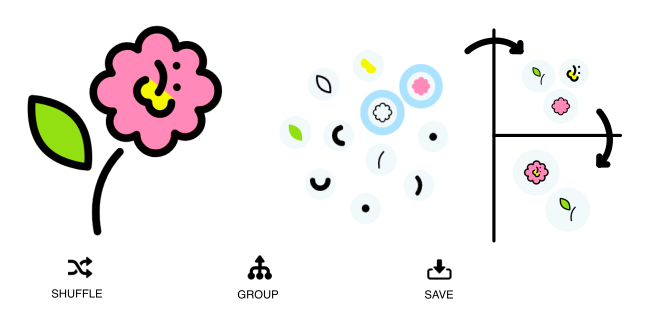
Figure 2. Annotation Interface: We show the graphic and its composing paths are side by side. The annotator selects paths by clicking on them directly in the graphic or by clicking on the individual bubbles containing paths. For example, the stroke and fill of the flower petals is selected (highlighted in blue). The group button is pressed to combine the chosen paths. The selected bubbles disappear and a new bubble representing the group is added. The annotator continues till only one bubble remains.

3. Trees for Perceptual Organization

3.1. Notation

By trees we refer to rooted trees or hierarchies. We setup some notation to ease the upcoming discussion. A tree, $T$ consists of a vertex set $V(T)$ and an edge set $E(T)$. A tree implicitly encodes a partial order among the vertex set. This is the ancestor-descendant relationship between vertices. Let $v_{1}\leq v_{2}$ denote that $v_{1}$ is a descendant of $v_{2}$. Further, let $v_{1}<v_{2}$ denote $v_{1}\leq v_{2}\land v_{1}\neq v_{2}$. Refer to $LCA(x,y)$ as the least common ancestor i.e. the deepest vertex that is also an ancestor of two vertices $x,y\in V$ in $T$. Let $Leaves(T)$ be the leaves of the tree and let $T(x)$ denote the subtree of $T$ rooted at vertex $x$.

3.2. Alternative Data Structures

We contrast trees with three alternatives: Graphs, $n$-ary Graphs and single level segmentations.

Graphics can be organized by recording all pairwise relationships between paths. However, obtaining this data from annotators is expensive. $O(n^{2})$ queries need to be made for a single graphic. Moreover, we can’t articulate relationships between more than two paths at a time.

$n$-ary Graphs (Mo et al., 2019) are hierarchies with edges between sibling vertices. They are more query-efficient than graphs and are an ideal candidate. As they are a strict generalization of trees, they are more expressive. However, it becomes harder to extract this information from lay people.

There is substantial prior work on segmentation, both for sketches (Yang et al., 2020; Li et al., 2019) and images (Lun et al., 2017). An algorithm designer has to explicitly choose what a group represents. Is the visual entity revealed by the group a noun, such as an eye, table, pen etc? Or is it merely elements having a common property, such as color, shape, size etc? A tree is better suited to the purpose since it can simultaneously record both high-level, semantic, and low-level, geometry-based relationships.

3.3. Argument for Trees

Trees naturally extend clusters and are easier to collect data for (Section 4) than Graphs and n-ary Graphs. They have other useful properties for the purpose of perceptual organization.

First, they can model the strength of the relationship between two percepts. In a tree, $T$, with two vertices, $a$ and $b$, $LCA(a,b)$ denotes the level at which the two percepts, represented by $a$ and $b$, are unified to form a distinct perceptual entity for an observer. The distance between the two vertices in the tree,

(1) $$Tdist(a,b)=Depth(a)+Depth(b)-2Depth(LCA(a,b)),$$

is inversely proportional to the strength of their relationship. We use this property to learn an embedding to compare different percepts (Section 5).

Second, they are efficient for selection. We hypothesize that any reasonable selection of $N$ paths can be well approximated by selecting $O(logN)$ vertices in a well organized tree. The set of $N$ paths can be written as a union of sets of sizes $2^{\lceil log_{2}N\rceil},2^{\lceil log_{2}N\rceil-1},\cdots,1$. We posit that a vertex in a well organized tree can approximate each subset. In other words, only a few vertices would have to be chosen at each level of the tree.

Finally, trees have been a mainstay in describing our visual system (Serre, 2014) and while they only serve as an approximation, it is likely that they endow inductive biases which reduce sample complexity. In fact, people have successfully trained low capacity recursive architectures for 3D shape generation and abstraction (Li et al., 2017; Mo et al., 2019).

4. VGTrees Dataset

We asked annotators to “assemble” each graphic hierarchically, starting from an unorganized collection of the paths in the graphic. This notion naturally maps artificial objects, such as chairs, tables, airplanes (Li et al., 2017; Mo et al., 2019; Yu et al., 2019; Wang et al., 2011) and indoor scenes (Li et al., 2019), but also generalises to other content well enough that it was useful to convey the task to the annotators.

We also gave annotators additional instructions to help ensure annotated hierarchies map well to usable semantics. We told them to create small-sized groups at a time, typically containing 2-5 subgroups, and we asked that they be able to rationalize their grouping decisions. We gave concrete examples of the latter, including, but not limited to: homogeneity in color or purpose, similarity in shape, and proximity. We also showed them a video where one of the authors performed the task.

# (graphic, tree) pairs	$1508$
Min paths	2
Max paths	103
Avg paths	13.85
Avg maximum depth in tree	4.95
Avg branching factor	2.32

Table 1. Dataset statistics at a glance

	# Graphics	$CTED\downarrow$		$FMI\uparrow$
				$d=3$	$d=2$	$d=1$
A v. A	47	0.270		0.128	0.504	0.863
A v. C	233	0.317		0.197	0.482	0.805
Overall	280	0.309		0.187	0.485	0.815

Table 2. We ran two studies to check for consistency among different annotators. We compared annotations by two of the authors, A v. A. We also compared annotations by one of the authors with crowd sourced ones, A v. C.. Each metric is in range $[0,1]$. Constrained Tree Edit Distance (lower is better), Fowlkes-Mallows Index (higher is better). Both show that there is consensus among annotators. In Section 7, we find that there is more consensus among human annotators, than between humans and algorithms.

We launched the annotation interface (Figure 2) as a web application, using graphics sourced from the publicly available OpenMoji dataset (Benedikt Groß and openmoji.org/about/#team, 2018). Table 1 shows relevant statistics of the dataset.

The majority of organizations ($\sim 85\%$) were created by the authors. To ensure that this did not cause the dataset to be biased due to annotators being subject experts or prejudiced towards their own methods, we ran two experiments. In the first one, two of the authors each organized 47 of the same graphics. In the second experiment, we crowd-sourced 233 organizations and compared them with our own. We evaluated the agreement between organization using Constrained Tree Edit Distance (CTED) (Zhang, 1996) and the Fowlkes-Mallows Index (FMI) (Fowlkes and Mallows, 1983). In Table 2, we find that while consistency between authors (A v. A) is better, as is to be expected, there is consistency between an author and crowd sourced annotations too (A v. C). In fact, according to CTED and FMI ($d=1$), there is more consistency between them than between our best model and human annotations.

5. Methodology

5.1. Overview

Our aim is to organize paths in a graphic into a tree in a way that makes it easy for humans to interact with it. We need to, recursively, decide pairs of paths to group. As the process goes on, grouped paths become candidates for further grouping.

We use the dataset (Section 4) to learn a function $\phi:V(T)\xrightarrow{}S^{64}$ that maps vertices in a tree to embeddings on a unit hypersphere. We enforce a monotonous mapping between grouping affinity and the cosine similarity of vertex embeddings.

The function $\phi$ can be used to make grouping decisions by a simple greedy strategy (Algorithm 1). Alternatively, we can design other inference strategies that are more suited for certain types of graphics. For example, it is often required that containment relationships be satisfied in the organization. Doing so is a straightforward extension of the scheme that we present, as we describe below.

5.2. Contrastive Learning for Grouping Affinity

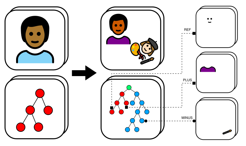
Figure 3. Each data point is a (graphic, tree) pair (left). These points go through a data augmentation pipeline (center). In this example, another data point is sampled and placed on the canvas. The path fills of the original graphic are perturbed in HSV space. The trees of the original data point (in red) and the new one (in blue) are combined using a new root vertex (in green). Three vertices are sampled (right). The REF and the PLUS vertices are closer to each other than to the MINUS vertex in the tree. Grouping affinity between vertices is learned via a contrastive loss.

We use the contrastive learning framework (Schroff et al., 2015; Oord et al., 2018; Wang and Isola, 2020) to learn $\phi$, parameterized by a neural network. A batch of triplets is constructed (Figure 3) with each triplet containing a reference $v$, a positive $v_{+}$ and a negative $v_{-}$ vertex. The reference and positive vertices have a higher grouping affinity than with the minus vertex. Using a modification of the contrastive loss, InfoNCE (Oord et al., 2018), we enforce that this holds true in the embedding space as well.

(2) $$\mathcal{L}=-\frac{e^{\phi(v)\cdot\phi(v_{+})/\tau}}{e^{\phi(v)\cdot\phi(v_{+})/\tau}+e^{\phi(v)\cdot\phi(v_{-})/\tau}}$$

We sample triplets on the basis of distance between vertices in the tree. Three vertices, $v_{1},v_{2},v_{3}$ are chosen at random from $V(T)$ and a permutation of $\{1,2,3\}$, $(i,j,k)$ is found such that:

(3) $$TDist(v_{i},v_{j})<TDist(v_{i},v_{k})\wedge TDist(v_{i},v_{j})<TDist(v_{j},v_{k})$$

Then $v_{i}$, $v_{j}$ and $v_{k}$ become the reference, positive and the negative vertices respectively. We found that adding the second proposition in the conjunction above was crucial in learning a good embedding (Section 8).

In early experiments we used a max margin loss for embeddings in euclidean space and found that training was unstable: our gradient clipping threshold was hit very often. In contrast, this behaviour wasn’t observed for the current setup. This has been observed before (Wang and Isola, 2020).

5.3. ReGroup Model

We now describe how we parameterize the embedding function $\phi$. The model has three components: location encoder, appearance encoder and context encoder. All three process vertices in the tree.

Each graphic is placed in a square canvas. Each vertex, $v\in V(T)$ in the corresponding tree represents a set of paths: $Leaves(T(v))$. We compute the axis oriented bounding boxes for each path. These are normalized to fit in a unit square. The extremities of this unit square represent those of the square canvas.

The location encoder is an MLP with two hidden layers. For a particular vertex, the tightest bounding box covering all its paths is computed and fed to the location encoder as input. The bounding box conveys information on the size and location of the vertex. Our experiments suggest that the location encoder, on its own, is surprisingly good at modeling grouping affinity.

The appearance encoder is an ImageNet pretrained ResNet18 (He et al., 2016). Its input is a raster of all paths in the vertex, composited on a square canvas. The square canvas covers the bounding boxes of the paths and includes some padding. The fc layer of the ResNet is modified so that instead of producing the logits for ImageNet classification, it produces a small dimensional vector.

Together, the location encoder and the appearance encoder convey the vertex’ visual attributes in a resolution independent manner. In order to incorporate contextual information of the vertex in the presence of the rest of the graphic, we add a context encoder.

The context encoder is based on the Fast R-CNN modification proposed by Mask R-CNN (Girshick, 2015; He et al., 2017). This module is another ImageNet pretrained ResNet18 equipped with the RoIAlign layer. Its input is a raster of the whole graphic and the vertex bounding box. The ResNet18 produces a feature map from the raster. The RoIAlign layer pools the features from the map in the region specified by the vertex bounding box. While these features are biased towards the region of the graphic containing the vertex, their receptive field is the whole graphic. In this sense, they encode how the vertex appears in the context of the whole graphic. Further, we make the same modification to $fc$ of this module as that for the appearance encoder.

All three modules described above output a $64D$ vector. These vectors are concatenated and processed by another MLP with two hidden layers to produce an embedding on $S^{64}$. The outputs of the individual modules are layer normalized (Ba et al., 2016) so that training progresses independently of the difference in initialization of the three modules and to force downstream layers to use all three of them.

5.4. Data Augmentation

By simple XML DOM manipulation, we can create new data points that help enforce desirable invariants. A nice consequence of working with the DOM is that the augmentations are much faster than ones in the raster domain. We list the five augmentations that form a part of our pipeline.

1. Rotational Transformation: The graphic is rotated around its center.

2. No Fill Transformation: We set all fill colours to empty to obtain line drawing.

3. Stroke Width and Opacity Jitter: We make strokes thicker or thinner. We also perturb the fill opacities.

4. HSV Jitter: We transform the path fills in HSV space.

5. Graphic Combination: We combine two graphics on the same canvas by placing them in non overlapping regions.

Grouping affinities, arguably, don’t change under any of these transformations. Figure 3 shows an example of applying the Rotational Transformation, HSV Jitter and Graphic Combination to the dataset. We use these augmentations in a probabilistic program. As a result, we generate a wide variety of training examples, each a product of zero or more of the augmentations described above.

Input: $\phi$, $N$ Paths in Graphic

Result: Tree $T$

$subtrees$ = [$path_{1},path_{2},\cdots,path_{N}$];

while length(subtrees) ¿ 1 do

       $subtreePairs$ = $combinations(subtrees,2)$;

       $maxSimilarity$ = $-\infty$;

       $bestPair$ = $undefined$;

       for $pair$ $in$ $subtreePairs$ do

             $(subtree_{1},subtree_{2})$ = $pair$;

             $e_{1}$ = $\phi(subtree_{1}.root)$;

             $e_{2}$ = $\phi(subtree_{2}.root)$;

             $sim$ = $e_{1}\cdot e_{2}$;

             if $sim<maxSimilarity$ then

                   $maxSimilarity$ = $sim$;

                   $bestPair$ = $pair$;

                  

             end if

            

       end for

      $(subtree_{1},subtree_{2})$ = $bestPair$;

       $subtrees.remove(subtree_{1})$;

       $subtrees.remove(subtree_{2})$;

       $subtrees.add(bestPair)$;

      

end while

$T$ = $subtrees.first$;

Algorithm 1 Greedy Tree Inference

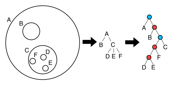
Figure 4. Containment guided tree inference. Given detected containment relationships between paths $A$-$E$ – $C$ contains $D,E,F$ and $A$ contains all the other paths (left) – we follow Fisher et al. (Fisher et al., 2021) to construct an initial coarse tree based on just these relationships (middle), and then expand each high-degree parent-children substructure to its final deeper form using our ReGroup neural grouping algorithm (right). The resulting structure respects all the containment constraints, while also reflecting the finer organization within each containment group.

5.5. Tree Inference

We present a simple $O(N^{3})$ algorithm (Algorithm 1), with $N$ being the number of paths in the graphic, for inferring an organizing hierarchy. Note that since our learned affinity function is cosine similarity in the embedding space, we can leverage efficient nearest neighbor search techniques (Guo et al., 2020) to accelerate inference in complex graphics. This is one of the principal reasons behind our design decision to target a standard inner-product metric, instead of having the network directly output a scalar affinity score for two paths.

We start with a set of trivial subtrees, each comprising just one node representing one of the $N$ individual paths. At each iteration, the two subtrees with the highest cosine similarity are chosen and merged via a newly-created common parent. The chosen pair is removed from the set and the combined subtree is added: the size of the set reduces by $1$. After $N-1$ steps, the complete hierarchy is obtained.

This setup is identical to hierarchical agglomerative clustering (HAC), with one crucial difference. Standard HAC algorithms provide only rudimentary means to directly compare internal vertices of the tree. The embedding of an internal vertex is approximated as some statistic (e.g. the mean) of the leaf vertex embeddings. Instead, we use a more powerful and accurate alternative: using $\phi$ to obtain embeddings for internal vertices as well. Hence, we embed each recursively obtained path grouping using the same fixed neural network module, making this a variant of recursive neural networks (Socher et al., 2011). The main difference from standard RvNNs is that the embedding of a parent node is computed by the neural net from the union of the leaf paths, not from the embeddings of its immediate children: computing the union is trivial, and we were able to make this work better in our experiments. It is not a “deep” model in the same way as a standard RvNN: however, since the network determines the topology of the tree, the embedding of an internal node is indeed influenced by the embeddings of its descendants.

We can extend this algorithm using the idea of containment groups from Fisher et. al. (Fisher et al., 2021). In many circumstances, containment is a strong indicator of grouping affinity. The algorithm proceeds by constructing a containment tree where parent paths contain child paths. (In general, it is possible for a path to be contained by more than one path. We heuristically choose only one path from among all containing paths as the parent.) Once the containment tree is constructed, each set of sibling paths is hierarchically grouped using the neural net-guided greedy strategy. The resulting subtree is then combined with the containing parent path to replace the containment-based parent-child substructure (Figure 4).

5.6. Implementation Details

We trained ReGroup for $28$ epochs. Each epoch had $25600$ triplets batched into sets of $32$. For validation we used $2560$ triplets. While the triplets sampled for training were different for each epoch, the ones for validation were fixed.

We used Adam (Kingma and Ba, 2014) with an initial learning rate of $0.0002$ which was decayed by $0.1$ every $7$ epochs. The temperature hyperparameter, $\tau$, was set to $0.1$.

The rasters for both the appearance encoder and the context encoder were $256$ by $256$ pixels. The conv1, bn1, layer1 and layer2 layers of the two ResNet18 were frozen. These are the module names as per the implementation in TorchVision. All the layers that weren’t ImageNet-pretrained were initialized using Kaiming Initialization (He et al., 2015a).

The graphics were rasterized using a GPU rasterizer, Pathfinder. Using this helped us avoid saving and loading rasters to/from disk. Training took $7$ hours on a single Nvidia Tesla T4 GPU.

6. Evaluation Metrics

In this section, we describe metrics that we chose to compare inferred trees against the ground truth.

6.1. Constrained Tree Edit Distance

Tree Edit Distances (Bille, 2005) give us a global measure for comparing two trees, $T_{1}$ and $T_{2}$. We briefly describe them under the framework of Tai Mappings (Kuboyama, 2007).

A Tai Mapping, $TM$ between $V(T_{1})$ and $V(T_{2})$, is a bijective mapping with the constraint that for any $(v_{1},w_{1}),(v_{2},w_{2})\in TM$:

(4) $$v_{1}\leq v_{2}\iff w_{1}\leq w_{2}$$

$TM$ respects the ancestor relationship in the two trees. For a $TM$, let $UM$ denote the set of vertices from both trees that are unmatched. Given a cost of relabeling, $r(a,b)$ and a cost of deletion, $d(a)$, the cost of $TM$ is defined as:

(5) $$cost(TM)=\sum_{(v,w)\in TM}r(v,w)+\sum_{v\in UM}d(v)$$

A desirable constraint in our problem setting is that two vertices have non overlapping paths in $T_{1}$, then the same holds for the corresponding mapped vertices in $T_{2}$. This is achieved by the Constrained Tai Mapping (Zhang, 1996). This is a Tai Mapping that satisfies: for any $(v_{1},w_{1}),(v_{2},w_{2}),(v_{3},w_{3})\in CTM$:

(6) $$v_{3}<LCA(v_{1},v_{2})\iff w_{3}<LCA(w_{1},w_{2})$$

We set delete and relabel costs to be:

(7) $$\begin{split}d(v)&=1\\ r(v,w)&=\frac{Leaves(T_{1}(v))\oplus Leaves(T_{2}(w))}{Leaves(T_{1}(v))\cup Leaves(T_{2}(w))}\end{split}$$

The minimum cost Constrained Tai Mapping gives us the Constrained Tree Edit Distance (CTED). When we report CTED, we make sure to normalize it by the total number of nodes in both trees so that it is in the range $[0,1]$.

6.2. Fowlkes-Mallows Index

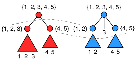
Figure 5. Fowlkes-Mallows Index is calculated by aligning two clusterings and measuring their precision and recall.

In addition to tree edit distances, we found it useful to track the $FMI$ (Fowlkes and Mallows, 1983). It indicates how well the inferred tree, $T_{1}$ and the ground truth tree, $T_{2}$, match at a coarse level. For example, as in Figure 5, $T_{1}$ and $T_{2}$ are cut at depth $d=1$ to obtain two clusterings over the paths i.e. the leaves of the trees. For a particular correspondence of clusters, say, $\{1,2,3\}\leftrightarrow\{1,2\}$ and $\{4,5\}\leftrightarrow\{4,5\}$, we categorize the pairs as follows:

1. True Positives: Number of pairs of paths that are in the same cluster on both sides of the mapping.

2. False Positives: Number of pairs of paths that belong to the same cluster on the right hand side of the mapping but not on the left.

3. False Negatives: Number of pairs of paths that belong to the same cluster on the left hand side but not on the right.

Based on these definitions, we define precision and recall. The maximum geometric mean of precision and recall, measured over all possible mappings, is the $FMI$ at that level.

7. Evaluation

In this section, we report comparisons between our method and the prior state-of-the-art: Suggero (Lindlbauer et al., 2013) and the very recent method of Fisher et al. (Fisher et al., 2021). We evaluate two versions of our method. The first is ReGroup where we explicitly enforce containment constraints as part of greedy tree inference. We also evaluate ReGroup-NoCG, where we drop the containment constraints. All comparisons, here, are done in a data-driven manner.

We conducted two tests. For the first one, we used different train-val-test splits of VGTrees (Section 4). For the second, we scraped partially organized graphics from the internet.

For the first test, we split VGTrees into 900 (graphic, tree) pairs for training, 200 for validation, and 200 for testing. We ensured that none of the graphics seen during training were included in the validation or test sets. The CTED and FMI scores (Table 3) for our method are significantly better than for Suggero and Fisher et. al.

For the second test, we scraped novel graphics from Publicdomainvectors.org. A good number of these graphics, encoded as SVGs (Bellamy-Royds et al., 2008), had group tags that indicated a grouping of a collection of graphical elements. We filtered for graphics containing three or more of such tags. Around $60\%$ of these graphics contained Inkscape metadata. This led us to believe that groups therein were created by humans, perhaps, for the purpose of editing. We manually inspected hundreds of these groups and found that they were largely consistent with our understanding of perceptual organization.

Since these graphics are only partially organized, we tried to find out whether the groups in the graphic are approximated by some vertex in our inferred tree. This score, referred to as Node Overlap, for a group $G$ and tree $T$, is:

(8) $$NO(G,T)=max_{v\in V(T)}IoU(Leaves(T(v)),G)$$

We evaluated these scores for 2 subsets of graphics, of size 200 each. We compare 3 grouping methods as in the first test. The scores (Table 3) are averaged over the 2 subsets and 3 methods.

We found that explicitly enforcing containment relationships was important for achieving the best score on Node Overlap: ReGroup improves upon the next best score of Fisher et al. However, this was not strictly true for CTED and FMI scores on VGTrees. One possible explanation is that annotators don’t always annotate consistently with respect to these relations, and the purely data-driven pipeline (ReGroup-NoCG) converges to fit these annotations (and hence also the characteristics of the VGTrees test set) more closely.

	$NO\uparrow$	$CTED\downarrow$		$FMI\uparrow$
				$d=3$	$d=2$	$d=1$
Suggero	$0.698\pm 0.02$	$0.448\pm 0.02$		$0.193\pm 0.02$	$0.385\pm 0.03$	$0.660\pm 0.01$
Fisher et. al.	$0.802\pm 0.00$	$0.420\pm 0.01$		$0.239\pm 0.02$	$0.432\pm 0.04$	$0.691\pm 0.04$
ReGroup-NoCG	$0.747\pm 0.01$	$\mathbf{0.343\pm 0.01}$		$0.288\pm 0.01$	$\mathbf{0.518\pm 0.03}$	$\mathbf{0.779\pm 0.02}$
ReGroup	$\mathbf{0.815\pm 0.01}$	$0.387\pm 0.01$		$\mathbf{0.296\pm 0.03}$	$0.504\pm 0.04$	$0.744\pm 0.03$

Table 3. Comparison of our method with prior heuristics-based perceptual grouping methods, using different metrics: Node Overlap (higher is better), Constrained Tree Edit Distance (lower is better), Fowlkes-Mallows Index (higher is better). Best values in bold. The error bars are 1 standard deviation with 6 trials for NO and 3 for the rest.

	$NO\uparrow$	$CTED\downarrow$		$FMI\uparrow$
				$d=3$	$d=2$	$d=1$
RG-NoCG	$0.747\pm 0.01$	${0.343\pm 0.01}$		$0.288\pm 0.01$	$\mathbf{0.518\pm 0.03}$	$\mathbf{0.779\pm 0.02}$
RG	${0.815\pm 0.01}$	$0.387\pm 0.01$		$\mathbf{0.296\pm 0.03}$	$0.504\pm 0.04$	$0.744\pm 0.03$
RG - DA	$0.805\pm 0.01$	$0.373\pm 0.01$		$0.264\pm 0.01$	$0.467\pm 0.03$	$0.699\pm 0.03$
RG-NoCG - DA	$0.709\pm 0.01$	$\mathbf{0.335\pm 0.01}$		$0.274\pm 0.01$	$0.494\pm 0.01$	$0.766\pm 0.01$
RG + AS	$0.809\pm 0.01$	$0.390\pm 0.01$		$0.258\pm 0.01$	$0.482\pm 0.02$	$0.704\pm 0.01$
RG-NoCG + AS	$0.730\pm 0.01$	$0.364\pm 0.01$		$0.234\pm 0.01$	$0.457\pm 0.01$	$0.704\pm 0.01$
RG - L	$0.799\pm 0.01$	$0.397\pm 0.01$		$0.284\pm 0.04$	$0.492\pm 0.04$	$0.723\pm 0.04$
RG-NoCG - L	$0.701\pm 0.02$	$0.363\pm 0.01$		$0.250\pm 0.01$	$0.480\pm 0.02$	$0.748\pm 0.02$
RG - A	$\mathbf{0.816\pm 0.01}$	$0.387\pm 0.01$		$0.280\pm 0.03$	$0.501\pm 0.04$	$0.747\pm 0.04$
RG-NoCG - A	$0.771\pm 0.01$	$0.352\pm 0.01$		$0.265\pm 0.01$	$0.511\pm 0.03$	$0.761\pm 0.02$
RG - C	$0.804\pm 0.01$	$0.401\pm 0.01$		$0.272\pm 0.04$	$0.486\pm 0.04$	$0.732\pm 0.04$
RG-NoCG - C	$0.704\pm 0.01$	$0.386\pm 0.02$		$0.225\pm 0.01$	$0.423\pm 0.01$	$0.706\pm 0.02$

Table 4. Ablations of our method: Node Overlap (higher is better), Constrained Tree Edit Distance (lower is better), Fowlkes-Mallows Index (higher is better). Best values in bold. Legend: RG: ReGroup; DA: Data Augmentation; AS: Alternative Sampling; L: Location Encoder; A: Appearance Encoder; C: Context Encoder . The error bars are 1 standard deviation with 6 trials for NO and 3 for the rest.

8. Ablations

In our ablation study, we evaluated the efficacy of data augmentation, our triplet sampling strategy, and the effect of each of our three encoders.

For data augmentation, our expectation was that data augmentation would aid generalization. Indeed, across all scenarios, models trained with data augmentation performed better than those without. The comparison Node Overlap score for ReGroup-NoCG, with and without data augmentation is particularly striking. Especially without the regularization of containment constraints, data augmentation helps achieve better scores on previously unseen graphics.

To measure the effect of our triplet sampling strategy, we added a second proposition in Equation 3 to further constrain the set of triplets. Specifically, we also enforce that $TDist(v_{+},v)<TDist(v_{+},v_{-})$. Removing this constraint is detrimental to training, as indicated by the RG + AS and RG-NoCG + AS scores in Table 4.

Finally, we tested the sensitivity of our results to each individual module in ReGroup. One by one, we reinitialized modules in the trained model to Kaiming Initialization. Any patterns learned were, thus, discarded. On the whole, we found that the contribution of each model was important to achieving good scores across metrics. However, surprisingly, reinitializing the appearance encoder seems to improve the Node Overlap scores for both variants of our method. Reinitializing the location encoder led to the biggest drop in Node Overlap scores.

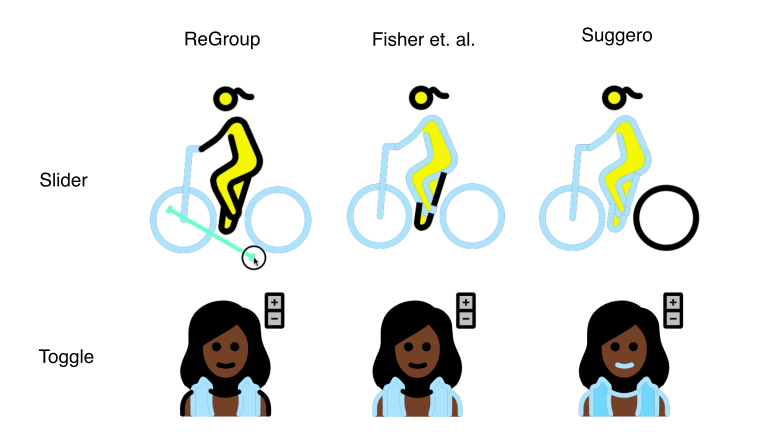
Figure 6. Visualizations of the Slider and Toggle selection tools. Please see the supplementary video for a visualization of the Scribble tool.

9. Applications

9.1. Click-Based Selection Tools

We made 3 variants of click-based selection tools. We made a Scribble tool, using Lazy Selection user interface  (Xu et al., 2012) to capture user intent, and using the inferred tree to generate meaningful selection suggestions by proposing internal nodes with the highest overlap with the scribbled line. Please see the supplementary video for example interactions with this tool.

We also made two versions of a tool that traverses the ancestor sequence from the selected path to the root of the tree. We call them Slider and Toggle.

To use Slider (Figure 6 (top)), the user clicks on an initial path and drags a slider in any direction. Parent groups are added to the current selection based on the length of the slider. In our initial user study we found that although the tool minimizes cursor travel, it is hard to understand. Users expect the direction of the drag to influence selection. This wasn’t the case in our implementation. Moreover, while the drag action was continuous, ancestor traversal was discrete. This made it hard for users to predict what is going to happen next.

In our final iteration, we developed the Toggle tool (Figure 6 (bottom)). After an initial click, the toggle bar comes up and users can select ancestors/descendants simply by clicking on plus/minus button. The interface is one-dimensional and discrete just like the traversal logic.

All three of these tools leverage the precomputed hierarchical structure to enable efficient selection.

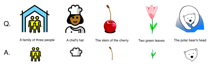
Figure 7. CLIP for text based selection: For each graphic (top row), and prompt (middle row), we find the node in the inferred tree most similar to the prompt using CLIP. The results (bottom row) are one of the top 3 most similar nodes for each (graphic, prompt) pair. Examples shown are from both graphics in VGTrees and the public domain. ReGroup infers trees with semantically meaningful nodes, appropriately matching the CLIP prompt.

9.2. Text-Based Selection Tool

We used inferred trees, in combination with CLIP (Radford et al., 2021), to create a text-based selection tool (Figure 7). CLIP is trained to jointly embed text and images in the same space. It is trained on a large dataset of (text, image) pairs and has impressive zero-shot capabilities.

Our prototype asks users for a text prompt. CLIP’s text encoder is used to find a feature vector for the prompt. CLIP’s image encoder embeds all nodes in the inferred tree in the same feature space. We find which node has the highest cosine similarity with the prompt feature vector. The top 3 most similar nodes are given to the user as suggestions.

The inferred tree lets us turn an exponential problem, of finding the optimal subset of paths for a prompt, into a linear one, where only the nodes in the tree need to be checked for prompt similarity. This relies on having tree nodes corresponding to most of the semantically meaningful entities of interest. As Figure 7 demonstrates, and the Node Overlap metric quantifies, this is frequently the case.

10. Limitations and Future Work

While our method achieves good qualitative and quantitative results on our test cases, its design induces several limitations. These are related to what relationships we can capture, and what hierarchies we can construct.

Because the greedy hierarchical clustering algorithm only considers pairs of nodes, we can only infer binary trees. This means we cannot directly represent e.g. the three blades of a ceiling fan or the spots on a ladybug in a single group: instead, they are grouped into an arbitrary binary tree. Because our node similarity measure is capable of evaluating similarity between leaves as well as groups, it should be possible to extend the greedy algorithm to use this information to add nodes to an existing group instead of creating a new one.

In the process of rendering the graphic for appearance and context encoders, the render order information is discarded as the paths are composited. This could potentially discard important hints on objects to be grouped based on e.g. being close in the render order. Future work could address this perhaps by adding a position encoding (Vaswani et al., 2017) to the embeddings.

We have in VGTrees, discovered several designs that violate our assumption that every path corresponds to an atomic design element. For instance, we found a graphic of two people standing side by side, where their torsos were represented by a single path. In this case, our model is unable to construct a semantically meaningful hierarchy. However, it is easy for a designer to fix this by splitting up such a compound object, and perhaps future work might discover a way of doing this automatically.

There are multiple possible ways of evaluating containment constraints, and which is the optimal one seems to be situationally dependent. For example, it is not clear how to decide which objects, if any, are contained by an open path. In our implementation, we make the pragmatic decision of connecting the end points of open paths, which is optimal in terms of our evaluation scores, but we can still find examples where this is not the right thing to do.

Moreover, always following containment constraints can give rise to false positives. Consider the example of a figure holding a water bottle in front of their torso. In this case the containment hint is spurious, because it represents the spatial relationship of separate objects rather than there being a single discrete object. But since the bottle is “contained” in the torso, it’ll be grouped with it before the torso is grouped with the hands. We hope there may be a data-driven solution for classifying these meaningful versus spurious containment relationships.

Our method only extracts what we believe to be semantic groups without attempting to actually recover the semantics by e.g. estimating vertex labels. As a result, we don’t know what a particular group represents. This also ultimately limits our ability to exploit the semantics of the groups to further improve grouping by considering e.g. the logical relationships between objects. Overcoming this is difficult, since the content is often highly stylised or abstract, and not all levels of a hierarchy are necessarily semantically meaningful.

Lastly, our method has not been stress-tested on complex graphics. It would also benefit from access to much larger training datasets. Unlike heuristic-based methods, whose performance is fixed, our data-driven approach has the potential to continuously improve as it is trained on more data.

11. Conclusion

In this paper we present a method to automatically organise vector graphics into hierarchical structures represented as trees, for the purposes of simplifying the manipulation of these graphics. We have proposed a data-driven similarity metric which we trained on the dataset we had gathered, and designed an algorithm to construct a hierarchy from this similarity information.

We evaluated our method against various baselines on a variety of vector data, focusing on the veracity of the induced hierarchy compared to the ground truth. Finally, we demonstrated prototype selection tools which take advantage of the hierarchical structure to facilitate rapid semantic selection.

References

- (1)
- Ba et al. (2016) Jimmy Lei Ba, Jamie Ryan Kiros, and Geoffrey E Hinton. 2016. Layer normalization. arXiv preprint arXiv:1607.06450 (2016).
- Barrett and Cheney (2002) William A Barrett and Alan S Cheney. 2002. Object-based image editing. In Proceedings of the 29th annual conference on Computer graphics and interactive techniques. 777–784.
- Bellamy-Royds et al. (2008) Amelia Bellamy-Royds, Bogdan Brinza, Chris Lilley, Dirk Schulze, David Storey, and Eric Willigers. 2008. SVG 2.0 Specification. https://www.w3.org/TR/SVG2/.
- Benedikt Groß and openmoji.org/about/#team (2018) Carlin MacKenzie Benedikt Groß, Daniel Utz and openmoji.org/about/#team. 2018. OpenMoji – Open source emojis for designers, developers and everyone else! https://github.com/hfg-gmuend/openmoji.
- Bille (2005) Philip Bille. 2005. A survey on tree edit distance and related problems. Theoretical Computer Science 337, 1 (2005), 217 – 239. https://doi.org/10.1016/j.tcs.2004.12.030
- Dhanuka et al. (2020) Praveen Kumar Dhanuka, Vineet Batra, Ankit Phogat, and Sumit Dhingra. 2020. Automatic vector graphic organization and asset extraction. In ACM SIGGRAPH 2020 Posters. 1–2.
- Fisher et al. (2021) Matthew Fisher, Vineet Agarwal, and Tarun Beri. 2021. Automatic Hierarchical Arrangement of Vector Designs. (2021).
- Fowlkes and Mallows (1983) E. B. Fowlkes and C. L. Mallows. 1983. A Method for Comparing Two Hierarchical Clusterings. J. Amer. Statist. Assoc. 78, 383 (1983), 553–569. https://doi.org/10.1080/01621459.1983.10478008 arXiv:https://www.tandfonline.com/doi/pdf/10.1080/01621459.1983.10478008
- Girshick (2015) Ross Girshick. 2015. Fast r-cnn. In Proceedings of the IEEE international conference on computer vision. 1440–1448.
- Girshick et al. (2011) Ross Girshick, Pedro Felzenszwalb, and David McAllester. 2011. Object Detection with Grammar Models. In NeurIPS, J. Shawe-Taylor, R. Zemel, P. Bartlett, F. Pereira, and K. Q. Weinberger (Eds.), Vol. 24.
- Gogia (2016) Sumit Gogia. 2016. Insight: interactive machine learning for complex graphics selection. Ph. D. Dissertation. Massachusetts Institute of Technology.
- Greff et al. (2016) Klaus Greff, Antti Rasmus, Mathias Berglund, Tele Hao, Harri Valpola, and Jürgen Schmidhuber. 2016. Tagger: Deep unsupervised perceptual grouping. In Advances in Neural Information Processing Systems. 4484–4492.
- Guo et al. (2020) Ruiqi Guo, Philip Sun, Erik Lindgren, Quan Geng, David Simcha, Felix Chern, and Sanjiv Kumar. 2020. Accelerating Large-Scale Inference with Anisotropic Vector Quantization. In Proceedings of the 37th International Conference on Machine Learning, Vol. 119.
- He et al. (2017) Kaiming He, Georgia Gkioxari, Piotr Dollár, and Ross Girshick. 2017. Mask r-cnn. In Proceedings of the IEEE international conference on computer vision. 2961–2969.
- He et al. (2015a) Kaiming He, Xiangyu Zhang, Shaoqing Ren, and Jian Sun. 2015a. Delving deep into rectifiers: Surpassing human-level performance on imagenet classification. In Proceedings of the IEEE international conference on computer vision. 1026–1034.
- He et al. (2015b) Kaiming He, Xiangyu Zhang, Shaoqing Ren, and Jian Sun. 2015b. Spatial pyramid pooling in deep convolutional networks for visual recognition. IEEE transactions on pattern analysis and machine intelligence 37, 9 (2015), 1904–1916.
- He et al. (2016) Kaiming He, Xiangyu Zhang, Shaoqing Ren, and Jian Sun. 2016. Deep residual learning for image recognition. In Proceedings of the IEEE conference on computer vision and pattern recognition. 770–778.
- Kingma and Ba (2014) Diederik P Kingma and Jimmy Ba. 2014. Adam: A method for stochastic optimization. arXiv preprint arXiv:1412.6980 (2014).
- Kuboyama (2007) Tetsuji Kuboyama. 2007. Matching and learning in trees. Doctoral Thesis, University of Tokyo (2007).
- Leitner and Haller (2011) Jakob Leitner and Michael Haller. 2011. Harpoon Selection: Efficient Selections for Ungrouped Content on Large Pen-Based Surfaces. In Proceedings of the 24th Annual ACM Symposium on User Interface Software and Technology (Santa Barbara, California, USA) (UIST ’11). Association for Computing Machinery, New York, NY, USA, 593–602. https://doi.org/10.1145/2047196.2047275
- Li et al. (2017) Jun Li, Kai Xu, Siddhartha Chaudhuri, Ersin Yumer, Hao Zhang, and Leonidas Guibas. 2017. Grass: Generative recursive autoencoders for shape structures. ACM Transactions on Graphics (TOG) 36, 4 (2017), 1–14.
- Li et al. (2018) Ke Li, Kaiyue Pang, Jifei Song, Yi-Zhe Song, Tao Xiang, Timothy M Hospedales, and Honggang Zhang. 2018. Universal sketch perceptual grouping. In Proceedings of the european conference on computer vision (ECCV). 582–597.
- Li et al. (2019) K. Li, K. Pang, Y. Song, T. Xiang, T. M. Hospedales, and H. Zhang. 2019. Toward Deep Universal Sketch Perceptual Grouper. IEEE Transactions on Image Processing 28, 7 (2019), 3219–3231. https://doi.org/10.1109/TIP.2019.2895155
- Li et al. (2019) Manyi Li, Akshay Gadi Patil, Kai Xu, Siddhartha Chaudhuri, Owais Khan, Ariel Shamir, Changhe Tu, Baoquan Chen, Daniel Cohen-Or, and Hao Zhang. 2019. Grains: Generative recursive autoencoders for indoor scenes. ACM Transactions on Graphics (TOG) 38, 2 (2019), 1–16.
- Lin et al. (2017) Tsung-Yi Lin, Piotr Dollár, Ross Girshick, Kaiming He, Bharath Hariharan, and Serge Belongie. 2017. Feature pyramid networks for object detection. In Proceedings of the IEEE conference on computer vision and pattern recognition. 2117–2125.
- Lindlbauer et al. (2013) David Lindlbauer, Michael Haller, Mark Hancock, Stacey D. Scott, and Wolfgang Stuerzlinger. 2013. Perceptual Grouping: Selection Assistance for Digital Sketching. In Proceedings of the 2013 ACM International Conference on Interactive Tabletops and Surfaces (St. Andrews, Scotland, United Kingdom) (ITS ’13). Association for Computing Machinery, New York, NY, USA, 51–60. https://doi.org/10.1145/2512349.2512801
- Lun et al. (2017) Zhaoliang Lun, Changqing Zou, Haibin Huang, Evangelos Kalogerakis, Ping Tan, Marie-Paule Cani, and Hao Zhang. 2017. Learning to Group Discrete Graphical Patterns. ACM Trans. Graph. 36, 6, Article 225 (Nov. 2017), 11 pages. https://doi.org/10.1145/3130800.3130841
- Luo et al. (2020) Tiange Luo, Kaichun Mo, Zhiao Huang, Jiarui Xu, Siyu Hu, Liwei Wang, and Hao Su. 2020. Learning to group: a bottom-up framework for 3d part discovery in unseen categories. arXiv preprint arXiv:2002.06478 (2020).
- Martinović and Van Gool (2013) Anđelo Martinović and Luc Van Gool. 2013. Earley Parsing for 2D Stochastic Context Free Grammars. Technical Report KUL/ESAT/PSI/1301. KU Leuven.
- Metzger (1936) Wolfgang Metzger. 1936. Laws of seeing. The MIT Press.
- Mo et al. (2019) Kaichun Mo, Paul Guerrero, Li Yi, Hao Su, Peter Wonka, Niloy Mitra, and Leonidas Guibas. 2019. StructureNet: Hierarchical Graph Networks for 3D Shape Generation. ACM Transactions on Graphics (TOG), Siggraph Asia 2019 38, 6 (2019), Article 242.
- Müllner (2011) Daniel Müllner. 2011. Modern hierarchical, agglomerative clustering algorithms. arXiv:1109.2378 [stat.ML]
- Noris et al. (2012) Gioacchino Noris, Daniel Sỳkora, Arik Shamir, Stelian Coros, Brian Whited, Maryann Simmons, Alexander Hornung, M Gross, and R Sumner. 2012. Smart scribbles for sketch segmentation. In Computer Graphics Forum, Vol. 31. Wiley Online Library, 2516–2527.
- Oord et al. (2018) Aaron van den Oord, Yazhe Li, and Oriol Vinyals. 2018. Representation learning with contrastive predictive coding. arXiv preprint arXiv:1807.03748 (2018).
- Perteneder et al. (2015) Florian Perteneder, Martin Bresler, Eva-Maria Grossauer, Joanne Leong, and Michael Haller. 2015. CLuster: Smart Clustering of Free-Hand Sketches on Large Interactive Surfaces. In Proceedings of the 28th Annual ACM Symposium on User Interface Software & Technology (Charlotte, NC, USA) (UIST ’15). Association for Computing Machinery, New York, NY, USA, 37–46. https://doi.org/10.1145/2807442.2807455
- Radford et al. (2021) Alec Radford, Jong Wook Kim, Chris Hallacy, Aditya Ramesh, Gabriel Goh, Sandhini Agarwal, Girish Sastry, Amanda Askell, Pamela Mishkin, Jack Clark, et al. 2021. Learning transferable visual models from natural language supervision. arXiv preprint arXiv:2103.00020 (2021).
- Saund and Moran (1994) Eric Saund and Thomas P. Moran. 1994. A Perceptually-Supported Sketch Editor. In Proceedings of the 7th Annual ACM Symposium on User Interface Software and Technology (Marina del Rey, California, USA) (UIST ’94). Association for Computing Machinery, New York, NY, USA, 175–184. https://doi.org/10.1145/192426.192494
- Schroff et al. (2015) Florian Schroff, Dmitry Kalenichenko, and James Philbin. 2015. Facenet: A unified embedding for face recognition and clustering. In Proceedings of the IEEE conference on computer vision and pattern recognition. 815–823.
- Serre (2014) Thomas Serre. 2014. Hierarchical Models of the Visual System. Encyclopedia of computational neuroscience 6 (2014), 1–12.
- Socher et al. (2011) Richard Socher, Cliff Chiung-Yu Lin, Andrew Y Ng, and Christopher D Manning. 2011. Parsing natural scenes and natural language with recursive neural networks. In ICML.
- Socher et al. (2013) Richard Socher, Alex Perelygin, Jean Wu, Jason Chuang, Christopher D Manning, Andrew Y Ng, and Christopher Potts. 2013. Recursive deep models for semantic compositionality over a sentiment treebank. In Proceedings of the 2013 conference on empirical methods in natural language processing. 1631–1642.
- Talton et al. (2011) Jerry O. Talton, Yu Lou, Steve Lesser, Jared Duke, Radomír Měch, and Vladlen Koltun. 2011. Metropolis Procedural Modeling. ACM Trans. Graph. 30, 2, Article 11 (April 2011), 14 pages. https://doi.org/10.1145/1944846.1944851
- Vaswani et al. (2017) Ashish Vaswani, Noam Shazeer, Niki Parmar, Jakob Uszkoreit, Llion Jones, Aidan N Gomez, Łukasz Kaiser, and Illia Polosukhin. 2017. Attention is all you need. In Advances in neural information processing systems. 5998–6008.
- Wang and Isola (2020) Tongzhou Wang and Phillip Isola. 2020. Understanding contrastive representation learning through alignment and uniformity on the hypersphere. In International Conference on Machine Learning. PMLR, 9929–9939.
- Wang et al. (2018) Xiaogang Wang, Bin Zhou, Haiyue Fang, Xiaowu Chen, Qinping Zhao, and Kai Xu. 2018. Learning to Group and Label Fine-Grained Shape Components. ACM Trans. Graphics (SIGGRAPH Asia 2018) 37, 6 (2018).
- Wang et al. (2011) Yanzhen Wang, Kai Xu, Jun Li, Hao Zhang, Ariel Shamir, Ligang Liu, Zhiquan Cheng, and Yueshan Xiong. 2011. Symmetry hierarchy of man-made objects. In Computer graphics forum, Vol. 30. Wiley Online Library, 287–296.
- Wertheimer (1938) Max Wertheimer. 1938. Laws of organization in perceptual forms. (1938).
- Xu et al. (2012) Pengfei Xu, Hongbo Fu, Oscar Kin-Chung Au, and Chiew-Lan Tai. 2012. Lazy Selection: A Scribble-Based Tool for Smart Shape Elements Selection. ACM Trans. Graph. 31, 6, Article 142 (Nov. 2012), 9 pages. https://doi.org/10.1145/2366145.2366161
- Yang et al. (2020) Lumin Yang, Jiajie Zhuang, Hongbo Fu, Kun Zhou, and Youyi Zheng. 2020. Sketchgcn: Semantic sketch segmentation with graph convolutional networks. arXiv preprint arXiv:2003.00678 (2020).
- Yu et al. (2019) Fenggen Yu, Kun Liu, Yan Zhang, Chenyang Zhu, and Kai Xu. 2019. Partnet: A recursive part decomposition network for fine-grained and hierarchical shape segmentation. In Proceedings of the IEEE/CVF Conference on Computer Vision and Pattern Recognition. 9491–9500.
- Zhang (1996) Kaizhong Zhang. 1996. A constrained edit distance between unordered labeled trees. Algorithmica 15, 3 (1996), 205–222.