Intriguing Findings of Frequency Selection for Image Deblurring

Abstract

Blur was naturally analyzed in the frequency domain, by estimating the latent sharp image and the blur kernel given a blurry image. Recent progress on image deblurring always designs end-to-end architectures and aims at learning the difference between blurry and sharp image pairs from pixel-level, which inevitably overlooks the importance of blur kernels. This paper reveals an intriguing phenomenon that simply applying ReLU operation on the frequency domain of a blur image followed by inverse Fourier transform, i.e., frequency selection, provides faithful information about the blur pattern (e.g., the blur direction and blur level, implicitly shows the kernel pattern). Based on this observation, we attempt to leverage kernel-level information for image deblurring networks by inserting Fourier transform, ReLU operation, and inverse Fourier transform to the standard ResBlock. 1 $\times$ 1 convolution is further added to let the network modulate flexible thresholds for frequency selection. We term our newly built block as Res FFT-ReLU Block, which takes advantages of both kernel-level and pixel-level features via learning frequency-spatial dual-domain representations. Extensive experiments are conducted to acquire a thorough analysis on the insights of the method. Moreover, after plugging the proposed block into NAFNet, we can achieve 33.85 dB in PSNR on GoPro dataset. Our method noticeably improves backbone architectures without introducing many parameters, while maintaining low computational complexity. Code is available at https://github.com/DeepMed-Lab/DeepRFT-AAAI2023.

Introduction

Image deblurring aims at removing blurring artifacts to recover sharp images (Cho et al. 2021). The blurring of an image can be caused by many factors, e.g., camera shake, objects movement, out-of-focus optics, etc. The blurry image leads to visually low quality and hampers subsequent high-level vision tasks, ranging from security, medical imaging to object recognition (Chen et al. 2020).

Figure 1: PNSR vs. computational cost on the GoPro dataset (Nah, Kim, and Lee 2017). Our method performs much better than baseline methods: MIMO-UNet (Cho et al. 2021) and NAFNet (Chen et al. 2022), and other state-of-the-arts.

Image deblurring by frequency domain operations was very popular decades ago, based on a simple assumption that image blur may be due to the Point Spread Function (PSF) of the sensor, sensor motion, and other reasons (Banham and Katsaggelos 1997). Thus, the motion blurred image is expressed by convolving a latent sharp image with the PSF, which can be most easily instantiated in the frequency domain (Chakrabarti, Zickler, and Freeman 2010; Xu, Zheng, and Jia 2013; Hu et al. 2014; Pan et al. 2016). Here we take a simple example and assume that the blur kernel does not vary spatially: $B(\omega)=F(\omega)G(\omega)+N(\omega)$, where $F(\omega)$, $G(\omega)$, $B(\omega)$ and $N(\omega)$ are Fourier transforms of the sharp image, the blur kernel (PSF), the blurry image and the sensor noise, respectively, and $\omega\in[-\pi,\pi]^{2}$. This gives us an important cue that frequency domain offers us abundant information on image deblurring tasks which should not be overlooked.

Deep networks are popular for their end-to-end learning ability. The field of image deblurring has made significant advances riding on the wave of deep networks. DeepDeblur (Nah, Kim, and Lee 2017), pioneers the technique of end-to-end trainable methods, directly mapping a blurry image to its paired sharp image by a Convolutional Neural Network (CNN). It designs a multi-scale architecture, and uses a modified residual network structure (He et al. 2016) called ResBlock (see Fig. 4 (a)) to focus on learning the difference between blurry and sharp image pairs. Thereafter, end-to-end learning strategy with ResBlock is proven to be effective in image deblurring, and becomes a mainstream approach in recent years (Tao et al. 2018; Zhang et al. 2019a; Gao et al. 2019; Zhang et al. 2019b; Park et al. 2020; Yuan, Su, and Ma 2020; Zamir et al. 2021; Chen et al. 2021; Zou et al. 2021; Purohit et al. 2021; Cho et al. 2021; Chen et al. 2022). But, these methods overlook the importance of blur kernels.

In this paper, we reveal an intriguing phenomenon that taking the inverse Fourier transform on frequency selection (e.g., ReLU on the frequency domain) of a blurry image acts as learning blur pattern from the blurry image, indicating the blur direction and blur level, implicitly showing the kernel pattern. The faithful blur kernel information provided by such operations motivates us to insert Fourier transform, ReLU, and inverse Fourier transform to the standard ResBlock to take advantages of both kernel-level and pixel-level features via fusing frequency-spatial dual-domain representations. Furthermore, we investigate ReLU on the frequency domain from a new perspective, and experiments show that setting different thresholds instead of $0+j0$ ($0+j0$ is for ReLU) for frequency selection give different deblurring results. With this new viewpoint, we find that adding convolution after Fourier transform helps the network modulate flexible thresholds for selecting frequencies and can further promote image deblurring performance. To sum up, we propose a new, efficient and plug-and-play ResBlock, termed as Residual (Res) Fast Fourier Transform (FFT)-ReLU Block, to replace standard ResBlock. Our Res FFT-ReLU Block inserts a FFT-ReLU stream, consisting of 4 simple operations: 2D real FFT, 1$\times$1 convolutions, ReLU and inverse 2D real FFT, into ResBlock.

The effectiveness of the Res FFT-ReLU Block is compared and verified by plugging in different architectures on three datasets: GoPro (Nah, Kim, and Lee 2017), HIDE (Shen et al. 2019) and RealBlur (Rim et al. 2020) datasets. Substantial ablation studies are conducted to explore insights of the FFT-ReLU stream. It is worth mentioning that after plugging the proposed stream to MIMO-UNet+ (Cho et al. 2021) and NAFNet (Chen et al. 2022), the new models, which are termed as FMIMO-UNet+ and FNAFNet, can achieve 33.52 dB and 33.85 dB respectively in terms of PSNR on GoPro dataset. Our method noticeably improves backbone architectures without introducing too many parameters, while maintaining low computational complexity. The PSNR vs. FLOPs (G) compared with state-of-the-art methods are shown in Fig. 1.

Related Works

Deep Image Deblurring

Deep learning methods have achieved significant success in image deblurring (Sun et al. 2015; Nah, Kim, and Lee 2017) as well as other low-level vision tasks such as image denoise (Cheng et al. 2021; Zamir et al. 2020), image deraining (Jiang et al. 2020) and image super-resolution (Mei, Fan, and Zhou 2021; Dong et al. 2016; Zhang et al. 2018b; Guo et al. 2020). Sun et al. (Sun et al. 2015) propose to estimate the spatially-varying kernels of motion blur by a CNN. But, since the characteristics of blur are complex, the blur kernel estimation method is not practical in real scenarios. Later, DeepDeblur (Nah, Kim, and Lee 2017) directly maps a blurry image to its sharp counterpart. Scale-recurrent network (Tao et al. 2018) proposes an encoder-decoder structure to yield training feasibility. Adversarial training(Kupyn et al. 2018, 2019; Zhang et al. 2020) and Recurrent Neural Networks(Zhang et al. 2018a; Park et al. 2020) also have been extensively studied. Most of these networks perform CNNs on the spatial domain to recover the sharp image. MAXIM (Tu et al. 2022) proposes MLP-based building blocks, which requires a big batch size for training. NAFNet (Chen et al. 2022) designs computationally efficient networks from the baseline, which even achieves 33.69 dB PSNR on GoPro. Instead of designing a brand-new end-to-end image deblurring architecture, we reveal an intriguing phenomenon on frequency selection, and shed new light on improving the deblurring performance by incorporating faithful information about the blur pattern.

Transformer/non-local has strong global context modeling ability and has shown its great promise in various computer vision tasks. Some transformer-based image restoration methods have been proposed, such as SwinIR (Liang et al. 2021), Restormer (Zamir et al. 2022) and Uformer (Wang et al. 2022). But the considerable computational complexity usually hampers their usage in efficient image restoration. We test the model of SwinIR (Liang et al. 2021) and Restormer (32.92 dB on GoPro) (Zamir et al. 2022) on GoPro dataset, which take 1.99s and 1.14s per image, respectively, even much slower than MPRNet, while our FMIMO-UNet (33.08 dB) takes 0.339s per image.

End-to-end Deblur Model with ResBlock

DeepDeblur (Nah, Kim, and Lee 2017) designs a residual block (ResBlock) based on Conv-ReLU-Conv structure. Thereafter, ResBlock has become one fundamental block in image deblurring (Tao et al. 2018; Zhang et al. 2019a; Park et al. 2020; Cho et al. 2021). Various efforts have been devoted to modifying the ResBlock, e.g., the content-aware processing module proposed by SAPHN (Suin, Purohit, and Rajagopalan 2020), the channel attention block proposed by MPRNet (Zamir et al. 2021), the HIN block proposed by HINet (Chen et al. 2021), and the dilated conv block proposed by SDWNet (Zou et al. 2021).

Applications of Fourier Transform

In recent years, some methods extract information from the frequency domain to fulfill different tasks (Chi et al. 2019; Rippel, Snoek, and Adams 2015; Zhong et al. 2018; Yang and Soatto 2020; Rao et al. 2021; Suvorov et al. 2022). FDA (Yang and Soatto 2020) swaps the low-frequency spectrum between images to mitigate the influence caused by the images’ style change for image segmentation. GFNet (Rao et al. 2021) learns long-term spatial dependencies in the frequency domain for image classification. LaMa (Suvorov et al. 2022) applies the structure of fast Fourier convolution (Chi, Jiang, and Mu 2020) to image inpainting. In image deblurring, SDWNet (Zou et al. 2021) introduces wavelet transform into deep networks. In this paper, we reveal an intriguing phenomenon of frequency selection for image deblurring.

Method

Empirical Findings of Frequency Selection via ReLU Operation

We will describe the main observation insights of this paper in this section. The blurry image can be modeled as convolving the latent sharp image with the blur kernel. For simplicity, we elaborate the deviation in 1D scenario. The “unknown” sharp image is defined as $f(t)=\left\{\begin{matrix}1&|t|<\tau\\ 0&|t|>\tau\\ \end{matrix}\right.$ The blur kernel of a simple motion blur can be denoted as $g(t)=\delta(t)+\delta(t+\epsilon)$, where $\delta(\cdot)$ is the Direct delta function, and $\epsilon$ is a very small value.

Remark 1: Based on the above assumption, let’s define a blurry image $b=g\otimes f$, where $\otimes$ means convolution, and we drop $t$ for simplicity. Taking the inverse Fourier transform (i.e., $\mathcal{F}^{-1}(\cdot)$) after ReLU (i.e., $\sigma(\cdot)$) on the blurry image in the frequency domain ($\mathcal{F}(\cdot)$ means Fourier transform) is written as $\hat{b}=\mathcal{F}^{-1}(\sigma(\mathcal{F}(b)))$, which can separate blur pattern component from other components. ReLU is applied to the real and imaginary parts respectively.

More details to support Remark 1 are given in the supplementary material. One can easily decompose $\hat{b}$ and obtain a separate component from $\hat{b}$ as $(\delta(t)+1/2(\delta(t-\epsilon)+\delta(t+\epsilon)))\otimes\mathcal{F}^{-1}(|\mathcal{F}(f(t))|)$.

Figure 2: Given a top-hat function $f$ on the left, its $\mathcal{F}^{-1}(|\mathcal{F}(f)|$ is plotted on the right, with obvious peaks, where $\mathcal{F}(\cdot)$ and $\mathcal{F}^{-1}(\cdot)$ mean discrete Fourier and inverse Fourier transform.

Figure 3: We use a circle image as an example for sharp image $f$. The image is blurred ($b$) by linear kernels with motion blur of different directions $\{0^{\circ},45^{\circ},90^{\circ},135^{\circ},180^{\circ}\}$, different blur levels and a mixture of blur. Blur kernel-like images are calculated by the equations below the image. The middle image of the sharp image is visualized for reference. See more details in the supplementary material about equations $\mathcal{F}^{-1}(\sigma(\mathcal{F}(f)))-f/2$ and $\mathcal{F}^{-1}(\sigma(\mathcal{F}(b)))-b/2$ (best viewed by zoom-in on screen).

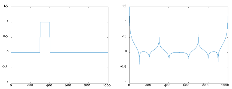
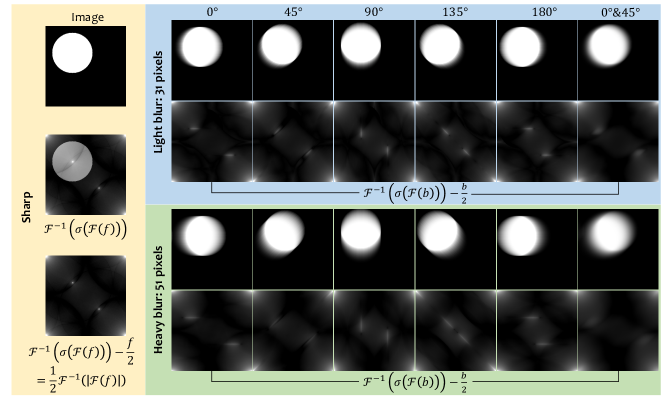
We observe that an absolute operation on Fourier transform of a top-hat function will produce peaks after inverse Fourier transform, as examples shown in Fig. 2. We plot the discrete Fourier transform. Based on the phenomenon revealed in Fig. 2, $\mathcal{F}^{-1}(\sigma(\mathcal{F}(g\otimes f)))$ will separate a component containing the convolution of $g$ and some peak values, when $f$ is a top-hat function.

Without loss of generality, we can extend Remark 1 to more complicated scenarios. Fig. 3 shows examples of feature selection derived from a clean and blurry images caused by blur kernels with different blur direction, blur levels and mixtures of blur. As may be observed, taking inverse Fourier transform on frequency selection via ReLU acts as a sort of learning blur pattern directly from the blurry image.

Figure 4: (a) ResBlock. (b) Insert simple FFT-ReLU stream into ResBlock. (c) Proposed Res FFT-ReLU Block, where the bottom stream is termed as FFT-ReLU stream.

Simple Fourier Transform with ReLU Stream

Basic Building Block for Image Deblurring

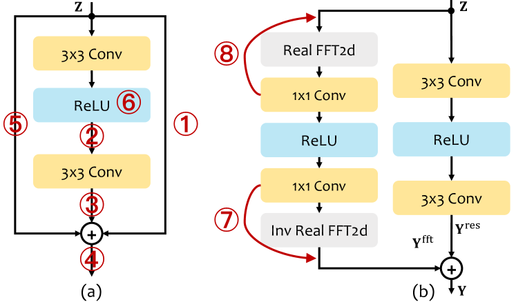
The residual building block in image deblurring tasks is called ResBlock. Specifically, standard ResBlock learns pixel-level features, consisting of two $3\times 3$ convolutional layers and one ReLU layer in between, as shown in Fig. 4 (a). Using inverse Fourier transform after selecting frequency from a blurry image $\mathcal{F}^{-1}(\sigma(\mathcal{F}(b)))$ generates blur patterns, implicitly showing the kernel pattern (see Eq. 3 in supplementary material and Fig. 3, $\mathcal{F}^{-1}(\sigma(\mathcal{F}(b)))$ can be considered as a linear combination of a blur pattern image $\mathcal{F}^{-1}(|\mathcal{F}(b)|)$ and $b$). If such operations can be inserted into an end-to-end image deblurring network, the network will be able to learn both kernel-level and pixel-level information. Many methods can be applied to fuse kernel-level blur pattern features generated by $\mathcal{F}^{-1}(\sigma(\mathcal{F}(b)))$ and the pixel-level features. Instead of designing a complicated fusion block, we simply replace the identity mapping by $\mathcal{F}^{-1}(\sigma(\mathcal{F}(\mathbf{Z})))$ for the sake of light computation, i.e., replace the identity mapping in Fig. 4(a) by the left most stream, termed as simple-FFT-ReLU stream in Fig. 4(b). The position of simple-FFT-ReLU stream w.r.t. the standard ResBlock (see Fig. 5(a)) can be changed, and our experiments show that fusing kernel-level and pixel-level features either in parallel or sequentially can boost the results (see Table 1).

Analysis of ReLU on Frequency Domain from A New Perspective

We analyze ReLU in frequency domain from another perspective. The phase and amplitude of a complex number $z=me^{j\beta}$ are $e^{j\beta}$ and $m\geq 0$ respectively. A Fourier transformed feature gives the phase and amplitude components. Applying ReLU (denoted as $\sigma(\cdot)$) on the frequency domain of a feature is defined as $\sigma(me^{j\beta})=m\sigma(e^{j\beta})$. This is considered as applying ReLU on the phase of the feature. As suggested by Pan (Pan et al. 2019), the phase of a blurry image plays an important role for deblurring, providing faithful information about the motion pattern. Applying ReLU indicates setting $T=0+j0$ as the selective threshold. What will happen if we change the threshold for frequency selection? As shown in Table 2 in the experiment, setting different thresholds on ReLU, i.e., $m\sigma(e^{j\beta}-\frac{T}{m})+T$, gives different results, e.g., $T=100(1+j)$ leads to a better result compared with original ReLU. A proper threshold for selecting frequency is important for deblurring. But $T$ has to be set manually. To let the network modulate flexible thresholds for selecting frequencies, convolution can be further added after Fourier transform. For the sake of simplicity, let $a\cdot ke^{j\beta}+b$ denote the feature after $1\times$1 conv in frequency, where $a$ and $b$ are learnable complex values. $m\sigma(e^{j\beta}-\frac{T}{m})+T$ is then replaced by $m\sigma(a\cdot e^{j\beta}+\frac{b}{m})$ (ReLU after convolution).

Res FFT-ReLU Block

From the above analysis, we propose a Residual Fast Fourier Transform with ReLU Block (Res FFT-ReLU Block) to replace the widely-used ResBlock. As shown in Fig. 4(c), different from Fig. 4(b), we keep the identity mapping which assists network training.

As shown in Fig. 4(c), besides a normal spatial residual stream, we simply add another stream based on a channel-wise FFT (Brigham and Morrow 1967). DFT is widely used in modern signal processing algorithms, whose 1D version can be derived by $X[k]=\sum_{n=0}^{N-1}x[n]e^{-j\frac{2\pi}{N}kn}$, where $x[n]$ is a sequence of $N$ complex numbers, $X[k]$ indicates the spectrum at the frequency $\omega_{k}=2\pi k/N$, and $j$ represent the imaginary unit. It is clear that the spectrum at any frequency has global information. Noted that the DFT of a real signal $x[n]$ is conjugate symmetric, i.e. $X[N-k]=\sum_{n=0}^{N-1}x[n]e^{-j\frac{2\pi}{N}(N-k)n}=X^{*}[k]$. The same applies to 2D DFT, which performs sequential row and column 1D DFT on a 2D signal whose size is $M\times N$, i.e., $X[M-u,N-v]=X^{*}[u,v]$. Since the results of a real array’s DFT has symmetric properties, the right half of the results can be derived from the left half. The FFT algorithms reduce the complexity and calculates the DFT in a more efficient way. Let $\mathbf{Z}\in\mathbb{R}^{H\times W\times C}$ be the input feature volume, where $H$, $W$, and $C$ indicate the height, width and channel of the feature volume. The left stream in Res FFT-ReLU Block, called FFT-ReLU stream (see Fig. 4(c)) is processed as follows:

• computes 2D real FFT of $\mathbf{Z}$ and obtain $\tilde{\mathbf{Z}}=\mathcal{F}(\mathbf{Z})\in\mathbb{C}^{H\times W/2\times C}$, where $\mathbb{C}$ means complex domain.

• uses two stacks of $1\times 1$ convolution layers (convolution operator $\otimes$) with a ReLU layer in between: $h(\tilde{\mathbf{Z}};\mathbf{\Theta}^{(1)},\mathbf{\Theta}^{(2)})=\text{ReLU}(\tilde{\mathbf{Z}}\otimes\mathbf{\Theta}^{(1)})\otimes\mathbf{\Theta}^{(2)}\in\mathbb{C}^{H\times W/2\times C}$, where $\mathbf{\Theta}^{(1)},\mathbf{\Theta}^{(1)}\in\mathbb{C}^{C\times C}$ are parameters in complex values, and $h(\cdot;\mathbf{\Theta}^{(1)},\mathbf{\Theta}^{(2)})$ is the network block parameterized by $\mathbf{\Theta}^{(1)}$ and $\mathbf{\Theta}^{(2)}$. We apply ReLU to the real and imaginary parts respectively.

• applies inverse 2D real FFT to transform $h(\tilde{\mathbf{Z}};\mathbf{\Theta}^{(1)},\mathbf{\Theta}^{(2)})$ back to spatial domain: $\mathbf{Y}^{\text{fft}}=\mathcal{F}^{-1}\left(h(\tilde{\mathbf{Z}};\mathbf{\Theta}^{(1)},\mathbf{\Theta}^{(2)})\right)\in\mathbb{R}^{H\times W\times C}$.

Then the final output of Res FFT-ReLU Block is calculated via $\mathbf{Y}=\mathbf{Y}^{\text{fft}}+\mathbf{Y}^{\text{res}}+\mathbf{Z}$, where $\mathbf{Y}^{\text{res}}$ uses the same computation as that in the original ResBlock. The code of realizing $\Theta^{(1)}$ on $\mathbf{Z}$ is:

weight_real=nn.Parameter(torch.Tensor(C, C))
weight_imag=nn.Parameter(torch.Tensor(C, C))
weight=torch.complex(weight_real,weight_imag)
Z_output=Z@weight #@ is matrix multiplication

Global Context Learning Ability

Convolution on Frequency Does Not Bring the Global Context Learning Ability

Mathematically, given $x[n]$, which is a sequence of $N$ numbers. For $S\times 1$ convolution on the spatial domain, weights are denoted as $w[a]$, where $a\in\mathcal{N}_{n}(S)$, and $\mathcal{N}_{n}(S)$ indicates a $S\times 1$ neighborhood of $x[n]$. We have $y=\sum_{a}x[n-a]\cdot w[a]$. If we conduct $S\times 1$ convolution on the frequency domain, we have $y=\mathcal{F}^{-1}(\sum_{a}X[k-a]w[a])=\sum_{a}w[a]\cdot x[n]\cdot e^{j2\pi an/N}$, where $X[k]$ is from Res FFT-ReLU Block section. This indicates that linear convolution operation on frequency domain is only used to extract features, which cannot introduce global context learning ability to the network.

ReLU on Frequency Brings the Global Context Learning Ability for the Network

ReLU is a non-linear operation. The output feature on the $r$th spatial location after converting to the spatial domain is calculated by $x[r]=\frac{1}{N}\sum_{k=0}^{N-1}\left(\sigma(\sum_{n=0}^{N-1}x[n]e^{-j2\pi kn/N})e^{j2\pi rk/N}\right)$. Since ReLU is nonlinear, unlike convolution, it is not possible to simplify this equation by eliminating any $x[n]$. Thus, introducing ReLU in the frequency domain brings the global context learning ability for the network. We will show in Table 1 that ReLU in frequency domain not always helps improve performance, whose location matters.

Experiments

Experimental Setup

Dataset

Three datasets are mainly evaluated: GoPro (Nah, Kim, and Lee 2017), HIDE (Shen et al. 2019) and RealBlur (Rim et al. 2020) datasets. Since existing methods adopt different experimental settings, we summarize them and report two groups of results: (I) train on 2,103 pairs of blurry and sharp images in GoPro dataset, and test on 1,111 image pairs in GoPro (follow (Cho et al. 2021)), 2,025 image pairs in HIDE (follow (Zamir et al. 2021)), 980 image pairs in RealBlur-R test set, and 980 image pairs in RealBlur-J test set (follow (Zamir et al. 2021)), respectively; (II) train on 3,758 image pairs in RealBlur-R, and test on 980 image pairs in RealBlur-R (follow (Zamir et al. 2021)), and train on 3,758 image pairs in RealBlur-J, and test on 980 image pairs in RealBlur-J (follow (Zamir et al. 2021)). Besides, we also show the effectiveness of Res FFT-ReLU Block on REDS dataset (Nah et al. 2021), with 24,000 and 3,000 images for training and testing, respectively (follow (Tu et al. 2022)).

Loss Function

We unify the loss function for all experiments. $\hat{\mathbf{S}}$, $\mathbf{S}$ and $\varepsilon$ denote the predicted sharp image, the groundtruth sharp image, and a constant value $10^{-3}$, respectively. Two kinds of loss functions are adopted: (1) Charbonnier loss (Zamir et al. 2021): $\mathcal{L}_{c}=\sqrt{||\hat{\mathbf{S}}-{\mathbf{S}}||^{2}+\varepsilon^{2}}$, and (2) Frequency Reconstruction (FR) loss (Cho et al. 2021; Tu et al. 2022): $\mathcal{L}_{fr}=||\mathcal{F}(\hat{\mathbf{S}})-\mathcal{F}(\mathbf{S})||_{1}$. Finally, the loss function is $\mathcal{L}=\mathcal{L}_{c}+\alpha_{1}\mathcal{L}_{fr}$, where $\alpha_{1}$ is a tradeoff-parameter and is empirically set to 0.01.

Implementation Details

We adopt the training strategy used in MPRNet (Zamir et al. 2021) unless otherwise specified. I.e., the network training hyperparameters (and the default values we use) are patch size (256$\times$ 256), batch size (16), training epoch (3,000), optimizer (Adam (Kingma and Ba 2015)), initial learning rate (2$\times$10^-4). The learning rate is steadily decreased to 1$\times$10^-6 using the cosine annealing strategy (Loshchilov and Hutter 2017). Following (Zamir et al. 2021), horizontal and vertical flips are randomly applied on patches for data augmentation. For testing, we adopt the same dataset slicing crop method as used in SDWNet (Zou et al. 2021), where we utilize a step of 256 to perform 256$\times$256 size sliding window slicing, and compensate slicing on the edge part.

Evaluation metric

The average performance of PSNR and SSIM over all testing sets are computed by using the official software released by (Zamir et al. 2021). We report number of parameters, FLOPs, and testing time per image (see supplementary material) on on a workstation with Intel Xeon Gold 6240C CPU, NVIDIA GeForce RTX 3090 GPU.

Position Ablation on Simple-FFT-ReLU Stream

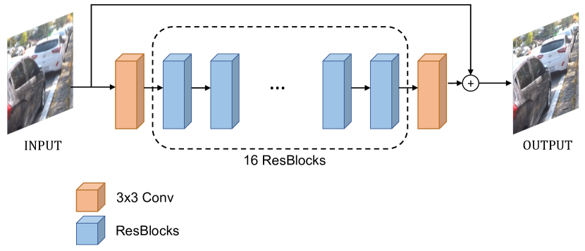
We discuss how the position of simple-FFT-ReLU stream on the ResBlock changes the deblurring performance. Experiments are conducted on GoPro dataset (Group I setting). The backbone architecture we use is a simplified version of DeepDeblur (Nah, Kim, and Lee 2017), which contains 16 ResBlocks, and termed as RSNet in the paper. As shown in Fig. 5(a), the position of simple-FFT-ReLU is changed w.r.t. ResBlock. Results are reported in Table 1. If we insert simple-FFT-ReLU in postion ⑥, the performance drops, compared with RSNet (27.78 vs. 28.06). If we replace the identity mapping by the simple-FFT-ReLU stream, PSNR increases compared with RSNet (29.51 vs. 28.06). This verifies our claim on the effectiveness of replacing identity mapping by simple FFT-ReLU stream, as marked in gray in Table 1. Based on this observation, we further change the threshold for filtering out frequencies. We conduct simple statistics and find that the real/imag values after FFT are mainly around $-10,000(1+j)$ to $+10,000(1+j)$. Thus, instead of setting $0+j0$ as the threshold, we try different thresholds, and also apply inverse ReLU (filter out frequency components larger than $0+j0$). Results are shown in Table 2. Inverse ReLU achieves similar results with ReLU (29.47 vs. 29.51). A positive threshold such as $+100(1+j)$ achieves better performance. Replacing ReLU by selecting high-/low- frequency components are not helpful at all, although all are non-linear operations. We also conduct ablation study on the position of 1$\times$1 convolution with simple-FFT-ReLU (see Fig. 5 (b)). Results are shown in Table 1.

Figure 5: Ablation on (a) the position of simple-FFT-ReLU, and (b) the position of 1$\times$1 convolution with simple-FFT-ReLU, where ① means we keep the identity mapping, and ⑥ indicates replacing ReLU with simple-FFT-ReLU. The others means the position where we insert simple-FFT-ReLU. ⑦ and ⑧ mean we put 1$\times$1 Conv before Real FFT2d or after inv Real FFT2d.

Table 1: Ablation on GoPro dataset with RSNet (Nah, Kim, and Lee 2017) for Fig. 5(a) (upper area) and Fig. 5(b) (bottom area). “$\times$” for ⑤ means the left stream is totally removed in Fig. 5(a). Result worse than RSNet is in italics.

①	②	③	④	⑤	⑥	⑦	⑧	PSNR	Params (M)
✓	$\times$	$\times$	$\times$	$\times$	$\times$	-	-	28.06	0.30
✓	✓	$\times$	$\times$	$\times$	$\times$	-	-	29.17	0.30
✓	$\times$	✓	$\times$	$\times$	$\times$	-	-	29.77	0.30
✓	$\times$	$\times$	✓	$\times$	$\times$	-	-	29.73	0.30
✓	$\times$	$\times$	$\times$	✓	$\times$	-	-	29.08	0.30
$\times$	$\times$	$\times$	$\times$	✓	$\times$	-	-	29.51	0.30
✓	$\times$	$\times$	$\times$	$\times$	✓	-	-	27.78	0.30
-	-	-	-	-	-	$\times$	$\times$	30.30	0.36
-	-	-	-	-	-	✓	$\times$	30.17	0.35
-	-	-	-	-	-	✓	✓	29.96	0.33

Table 2: Ablation on GoPro dataset with RSNet (Nah, Kim, and Lee 2017), for selecting frequency by different thresholds (upper), or replacing ReLU by high/low frequency selection (bottom) for the setting highlighted in Table 1.

Thre	Freq	PSNR
$-1000(1+j)$	-	28.71
$+1000(1+j)$	-	29.32
$-100(1+j)$	-	28.78
$+100(1+j)$	-	29.60
inv. ReLU	-	29.47
-	HF (1/8)	27.81
-	LF (1/8)	27.83

Figure 6: Visualization of example features of three layers of different networks. In each layer, to maximize the neuron on location $[\frac{1}{4}H,\frac{1}{4}W]$, we show visualizations from one random gradient descent run for channel $C=16$.

Ablation Study on FFT-ReLU Stream

Table 3: Ablation on FFT-ReLU stream on GoPro dataset with RSNet (Nah, Kim, and Lee 2017). “Real” means the weights in 1$\times$1 convolution are all real values, instead of the default complex values. “Concat” means after applying FFT, we concatenate the real part $\mathcal{R}(\mathcal{F}(\mathbf{Z}))$ and the imaginary part $\mathcal{I}(\mathcal{F}(\mathbf{Z}))$ along the channel dimension, so the weights of subsequent convolution operations are all real values. Gray areas indicate RSNet and RSNet w/ FFT-ReLU stream. Results worse than RSNet are in italics.

ResBlock		FFT-ReLU Stream					PSNR	Params
$\mathbf{Z}$	$\mathbf{Y}^{\text{res}}$	FFT	Conv	ReLU	Conv	iFFT		(M)
✓	✓	$\times$	$\times$	$\times$	$\times$	$\times$	28.06	0.30
$\times$	$\times$	✓	✓	✓	✓	✓	25.64	0.07
✓	$\times$	✓	✓	✓	✓	✓	26.00	0.07
✓	✓	$\times$	✓	✓	✓	$\times$	28.16	0.33
✓	✓	✓	$\times$	✓	$\times$	✓	29.08	0.30
✓	✓	✓	✓	$\times$	✓	✓	28.59	0.36
✓	✓	✓	✓	$\times$	$\times$	✓	28.60	0.33
✓	✓	✓	Real	✓	Real	✓	29.91	0.33
✓	✓	✓	✓	✓	$\times$	✓	30.06	0.33
✓	✓	✓	✓	✓	✓	✓	30.30	0.36
✓	✓	✓	✓	GeLU	✓	✓	30.42	0.36
✓	✓	✓	Concat	✓	Concat	✓	30.32	0.43
✓	✓	✓	3$\times$3	✓	3$\times$3	✓	31.15	1.48

Quantitative Results

We conduct extensive ablation study on GoPro dataset (Group I setting) to have a thorough investigation on the proposed FFT-ReLU stream. We can summarize the following conclusions from Table 3. (1) Using RSNet with only our FFT-ReLU stream leads to obvious performance drop, compared with RSNet (25.64 vs. 28.06), but adding FFT-ReLU stream to RSNet leads to significant improvement (30.30 vs. 28.06). This indicates that our FFT-ReLU stream is an add on stream, which should be trained in conjunction with the pixel-level spatial domain CNN. We will illustrate the reason by visualizing neurons in the next subsection. (2) It is expected to see that w/o ReLU w/ two 1$\times$1 convolution layers, the performance does not change too much, compared with RSNet (28.59 vs. 28.06). (3) If we change the complex convolution into real convolution, the performance drops a little due to the decrease of parameter numbers (29.91 vs. 30.30). (4) Noted that we propose a complex convolution in frequency domain. An alternative is to first concatenates the real part $\mathcal{R}(\mathcal{F}(\mathbf{Z}))$ and the imaginary part $\mathcal{I}(\mathcal{F}(\mathbf{Z}))$ along the channel dimension to acquire $\tilde{\mathbf{Z}}=\mathcal{R}(\mathcal{F}(\mathbf{Z}))\odot_{C}\mathcal{I}(\mathcal{F}(\mathbf{Z}))\in\mathbb{R}^{H\times W/2\times 2C}$, where $\odot_{C}$ represents concatenation through the channel dimension. Then we can simply use two stacks of $1\times 1$ convolution layers (convolution operator $\otimes$) with a ReLU layer in between: $h(\tilde{\mathbf{Z}};\mathbf{\Theta}^{(1)}_{\text{real}},\mathbf{\Theta}^{(2)}_{\text{real}})=\text{ReLU}(\tilde{\mathbf{Z}}*\mathbf{\Theta}^{(1)}_{\text{real}})\otimes\mathbf{\Theta}^{(2)}_{\text{real}}\in\mathbb{R}^{H\times W/2\times 2C}$. The inverse 2D real FFT can be applied afterwards. We term this alternative as “Concat”. Using Concat, the weights in convolution are all real values, and the performance does not change compared with our complex convolution (30.32 vs. 30.30), but the number of parameters increases. (5) We further replace 1$\times$1 convolution by 3$\times$3 convolution, which can be easily implemented in “Concat” setting. A further improvement is oberved (31.15 vs. 30.32). But, Concat 3$\times$3 increases the model parameters by 4 times, compared with Concat 1$\times$1.

Visualizations of Neurons

We visualize neurons to better understand how our FFT-ReLU stream works. In (Yosinski et al. 2015), the learned features computed by individual neurons at any layer of the network can be visualized by generating the input image such that the corresponding neurons activation value is maximized. Similarly, given a feature volume $\mathbf{Z}_{i}\in\mathbb{R}^{H\times W\times C}$ in Layer $i$, where $H$, $W$ and $C$ mean the height, width and the channel, we show visualizations of neurons on spatial location of $[\frac{1}{4}H,\frac{1}{4}W]$ from one random gradient descent run for $C=16$ in Layer 1, 8, 16, using a public repository. As shown in Fig. 6, to maximize the neuron on $[\frac{1}{4}H,\frac{1}{4}W]$, RSNet only gathers information from its local neighborhood. RSNet w/ only FFT-ReLU stream can learn global context, but using only FFT-ReLU stream lacks pixel-level localization ability, i.e., there is not a clear activation region on $[\frac{1}{4}H,\frac{1}{4}W]$. This explains the reason why it can only obtain $26.00$ dB in PSNR in Table 3. RSNet w/ FFT-ReLU stream can learn both kernel-level and pixel-level representations. Another interesting observation is that though FFT-ReLU stream has the ability to learn global context, in the lower layers, e.g., Layer 1, local information is more important, like Transformer (Raghu et al. 2021). Other details are provided in the supplementary material.

Evaluation of Res FFT-ReLU Block

Table 4: Evaluation of Res FFT-ReLU Block (Group I setting) in PSNR. FFT means the ResBlock is replaced by Res FFT-ReLU Block. $\times$ means the original architecture. All models are trained by ourselves for fair comparison.

Model	FFT	GoPro	HIDE	Params (M)	FLOPs (G)
Deep Deblur	$\times$	31.15	29.17	11.71	336.03
	✓	32.37$\uparrow$1.22	30.86$\uparrow$1.69	12.65	363.19
RSNet	$\times$	28.06	26.01	0.30	19.48
	✓	30.30$\uparrow$2.24	28.87$\uparrow$2.86	0.36	23.84
U-Net	$\times$	29.20	27.15	0.62	12.18
	✓	30.39$\uparrow$1.19	28.71$\uparrow$1.56	0.76	14.86
MPRNet	$\times$	31.09	29.66	2.14	80.70
-small	✓	32.50$\uparrow$1.41	30.82$\uparrow$1.16	2.43	94.24
MIMO-UNet	$\times$	31.90	29.62	6.80	67.17
	✓	32.71$\uparrow$0.81	30.85$\uparrow$1.23	8.17	80.21
NAFNet32	$\times$	32.95	30.60	17.1	16.00
	✓	33.12$\uparrow$0.17	30.76$\uparrow$0.16	17.8	23.10

Quantitative Results

Res FFT-ReLU Block is plug-and-play. We plug it into various architectures: DeepDeblur (Nah, Kim, and Lee 2017); U-Net (one backbone network used in MPRNet (Zamir et al. 2021)); MPRNet-small (Zamir et al. 2021), whose number of channels is three times smaller than original MPRNet due to limited computation resource; MIMO-UNet (Cho et al. 2021); NAFNet (Chen et al. 2022). NAFNet uses a different ResBlock, and we show the building block of NAFNet w/ Res FFT-ReLU Block in the supplementary material. PSNRs on GoPro and HIDE datasets in Group I setting are summarized in Table 4. Replacing ResBlock by our Res FFT-ReLU Block leads to remarkable performance gains in various architectures. Besides, RSNet and RSNet w/ Res FFT-ReLU Block on REDS dataset are tested. Results are 26.78 and 27.79$\uparrow$1.01 dB respectively.

Evaluation of FMIMO-UNet and FNAFNet

Table 5: Comparison on GoPro, HIDE and RealBlur datasets (Group I and II settings). Group II results are with $\mathparagraph$.

	GoPro	HIDE	RealBlur-R	RealBlur-J
Method	PSNR SSIM	PSNR SSIM	PSNR SSIM	PSNR SSIM
Xu et al. (CVPR’13)	21.00 0.741	-	34.46 0.937	27.14 0.830
Hu et al. (CVPR’14)	-	-	33.67 0.916	26.41 0.803
Pan et al. (CVPR’16)	-	-	34.01 0.916	27.22 0.790
Nah et al. (CVPR’17)	29.08 0.914	25.73 0.874	32.51 0.841	27.87 0.827
SRN (CVPR’18)	30.26 0.934	28.36 0.915	35.66 0.947	28.56 0.867
Zhang et al. (CVPR’18)	29.19 0.931	-	35.48 0.947	27.80 0.847
DeblurGAN (CVPR’18)	28.70 0.858	24.51 0.871	33.79 0.903	27.97 0.834
DeblurGAN-v2 (ICCV’19)	29.55 0.934	26.61 0.875	35.26 0.944	28.70 0.866
Gao et al. (CVPR’19)	30.90 0.935	29.11 0.913	-	-
DMPHN (CVPR’19)	31.20 0.940	29.09 0.924	35.70 0.948	28.42 0.860
RADN (AAAI’20)	31.76 0.953	-	-	-
Suin et al. (CVPR’20)	31.85 0.948	29.98 0.930	-	-
SVDN (CVPR’20)	29.81 0.937	-	-	-
DBGAN (CVPR’20)	31.10 0.942	28.94 0.915	33.78 0.909	24.93 0.745
MT-RNN (ECCV’20)	31.15 0.945	29.15 0.918	35.79 0.951	28.44 0.862
MPRNet (CVPR’21)	32.66 0.959	30.96 0.939	35.99 0.952	28.70 0.873
MIMO-UNet (ICCV’21)	31.73 0.951	29.28 0.921	35.47 0.946	27.76 0.836
MIMO-UNet+ (ICCV’21)	32.45 0.957	29.99 0.930	35.54 0.947	27.63 0.837
MIMO-UNet++ (ICCV’21)	32.68 0.959	-	-	-
SPAIR (ICCV’21)	32.06 0.953	30.29 0.931	-	28.81 0.875
HINet (CVPRW’21)	32.71 0.959	-	-	-
Restormer (CVPR’22)	32.92 0.961	31.22 0.942	36.19 0.957	28.96 0.879
Uformer (CVPR’22)	33.06 0.967	30.90 0.953	36.19 0.956	29.09 0.886
NAFNet32 (ECCV’22)	32.85 0.959	30.60 0.936	35.97 0.951	28.75 0.875
NAFNet64 (ECCV’22)	33.69 0.967	31.32 0.943	-	-
FMIMO-UNet-small	32.50 0.958	30.65 0.937	35.92 0.952	28.58 0.864
FMIMO-UNet	33.08 0.962	31.19 0.943	35.96 0.953	28.72 0.871
FMIMO-UNet+	33.52 0.965	31.66 0.946	36.11 0.955	28.88 0.880
FNAFNet32	33.12 0.962	30.76 0.938	36.07 0.955	28.78 0.879
FNAFNet64	33.85 0.967	31.12 0.944	-	-
DeblurGAN-v2 $\mathparagraph$ (ICCV’19)	-	-	36.44 0.935	29.69 0.870
SRN $\mathparagraph$ (CVPR’18)	-	-	38.65 0.965	31.38 0.909
MPRNet $\mathparagraph$ (CVPR’21)	-	-	39.31 0.972	31.76 0.922
FMIMO-UNet $\mathparagraph$	-	-	40.01 0.972	32.65 0.931
FMIMO-UNet+ $\mathparagraph$	-	-	40.01 0.973	32.63 0.933

MIMO-UNet and NAFNet are most recent ResBlock-based models with remarkable speed advantages among existing networks. We design FMIMO-UNet based on MIMO-UNet and MIMO-UNet+, acquiring FMIMO-UNet and FMIMO-UNet+. Besides, we reduce the number of Res FFT-ReLU Block to 4 for each encoder block and decoder block, and obtain an extra model termed as FMIMO-UNet-small. We design FNAFNet based on NAFNet. FMIMO-UNets and FNAFNet are compared with other state-of-the-arts in Table 5. Note that due to the limited computation resource, Res FFT-ReLU block is only added to a few encoder/decoder blocks. We set the batch size to 32 for both FNAFNet32 and FNAFNet64. See detailed analysis, computational cost comparisons and visualizations in the supplementary material.

Conclusion

In this paper, we reveal an intriguing phenomenon that frequency selection can provide faithful information about the blur pattern. With this viewpoint, we propose a plug-and-play block called Res FFT-ReLU Block based on FFT-ReLU stream. Res FFT-ReLU Block allows the image-wide receptive field which is able to capture the long-term interaction. Plugging Res FFT-ReLU Block into MIMO-UNet and NAFNet achieves remarkable superior performance compared with state-of-the-arts, on three well-known public image deblurring datasets.

Appendix A Appendix

Analysis of Remark 1

In this section, we provide the Analysis for Remark 1. For simplicity, we elaborate the deviation in 1D scenario. The “unknown” sharp image is defined as $f(t)=\left\{\begin{matrix}1&|t|<\tau\\ 0&|t|>\tau\\ \end{matrix}\right.$ The blur kernel of a simple motion blur can be denoted as $g(t)=\delta(t)+\delta(t+\epsilon)$, where $\delta(\cdot)$ is the Direct delta function, and $\epsilon$ is a very small value.

Analysis. Taking the inverse Fourier transform (denoted as $\mathcal{F}^{-1}(\cdot)$) after ReLU (denoted as $\sigma(\cdot)$, applied on real part and imaginary part separately) on the blurry image (denoted as $b$) in the frequency domain (Fourier transform is denoted as $\mathcal{F}(\cdot)$) can be formulated as:

$$\hat{b}=\mathcal{F}^{-1}(\sigma\left(\mathcal{F}(b)\right))$$ (1)

$$=\mathcal{F}^{-1}\left(\frac{\mathcal{F}(b)+\left|\mathcal{F}(b)\right|}{2}\right)$$ (2)

$$=\frac{b}{2}+\frac{1}{2}\mathcal{F}^{-1}(|\mathcal{F}(b)|)$$ (3)

$$=\frac{b}{2}+\frac{1}{2}\mathcal{F}^{-1}(\left|\mathcal{F}(g(t)\otimes f(t))\right|)$$ (4)

$$=\frac{b}{2}+\frac{1}{2}\mathcal{F}^{-1}\left(\left|\mathcal{F}(g(t))\cdot\mathcal{F}(f(t))\right|\right)$$ (5)

$$=\frac{b}{2}+\frac{1}{2}\mathcal{F}^{-1}(\left|\big{(}1+\cos(\omega\epsilon)+j\sin(\omega\epsilon)\big{)}\cdot\mathcal{F}(f(t))\right|)$$ (6)

$$=\frac{b}{2}+\frac{1}{2}\mathcal{F}^{-1}\left((1+\cos(\omega\epsilon))|\mathcal{F}(f(t))|\right)$$

$$~{}~{}~{}+\frac{1}{2}\mathcal{F}^{-1}(\left|j\sin(\omega\epsilon)\mathcal{F}(f(t))\right|)$$ (7)

$${=\frac{1}{2}\left(\delta(t)+\frac{1}{2}\left[\delta(t-\epsilon)+\delta(t+\epsilon)\right]\right)\otimes\mathcal{F}^{-1}(|\mathcal{F}(f(t))|)}$$

$$+\frac{1}{2}\mathcal{F}^{-1}(\left|j\sin(\omega\epsilon)\mathcal{F}(f(t))\right|)+\frac{b}{2}.$$ (8)

Note that $|\cdot|$ denotes conducting absolute operation on real part and imaginary part separately. According to Eq. 8, one can simply extract component $\left(\delta(t)+\frac{1}{2}\left[\delta(t-\epsilon)+\delta(t+\epsilon)\right]\right)\otimes\mathcal{F}^{-1}(|\mathcal{F}(f(t))|)$ from $\hat{b}$, which contains blur pattern. As shown in Fig. 2 in the paper, $\mathcal{F}^{-1}(|\mathcal{F}(f(t))|)$ produces peaks, which are caused by the $|\cdot|$ operation. Thus, $\hat{b}$ contains a blur pattern component: the convolution of the blur kernel $g(t)$ and some decomposed peak values. This component implicitly shows the kernel pattern.

Supplementary for Experiments

Network Structure

The Structure of RSNet

The backbone architecture we use in our ablation study is a simplified version of DeepDeblur (Nah, Kim, and Lee 2017), which contains 16 ResBlocks. We term it as RSNet, whose structure is illustrated in Fig. 7.

Figure 7: The structure of RSNet.

Building Block of NAFNet w/ Res FFT-ReLU

Figure 8: Building block of NAFNet w/ Res FFT-ReLU.

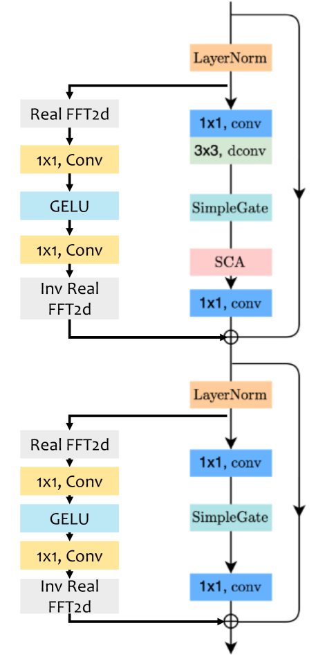
NAFNet (Chen et al. 2022) uses a different ResBlock compared with Fig. 4(a) in the paper. Thus, we add the proposed FFT-ReLU stream in a slightly different way. As shown in Fig. 8, the proposed Res FFT-ReLU block of FNAFNet consists of two FFT-ReLU streams.

In NAFNet, the computation is mainly conducted in the $5$th blocks. Noted that because of our limited computation resource, for FNAFNet32, we add Res FFT-ReLU block to the first three encoder blocks and their skip connected decoder blocks. For FNAFNet64, we only add Res FFT-ReLU block to the first encoder block and its skip connected decoder block.

Table 6: Ablation on FFT-ReLU stream on GoPro dataset (Nah, Kim, and Lee 2017) with RSNet (Nah, Kim, and Lee 2017) (16 ResBlocks). Let’s assume the height of a feature channel is $H$. “HF (1/4)” or “LF (1/4)” indicates after FFT, we only keep the high-frequency component which is outside or low-frequency component which is inside the circle with the radius of $\frac{1}{4}H$, respectively. “Layer 1 $\sim$ Layer 8” denotes we only add FFT-ReLU stream on the first 8 ResBlocks. Gray areas indicate conventional RSNet and RSNet w/ FFT-ReLU stream, as shown in Fig. 9. Results worse than conventional RSNet are in italics.

ResBlock		FFT-ReLU Stream
$\mathbf{Z}$	$\mathbf{Y}^{\text{res}}$	FFT	Conv	ReLU	Conv	iFFT	PSNR	Params (M)
✓	✓	$\times$	$\times$	$\times$	$\times$	$\times$	28.06	0.30
✓	✓	✓	✓	✓	✓	✓	30.30	0.36
✓	✓	HF (1/4)	✓	✓	✓	✓	28.64	0.36
✓	✓	LF (1/4)	✓	✓	✓	✓	30.44	0.36
✓	✓	HF (1/8)	✓	✓	✓	✓	29.03	0.36
✓	✓	LF (1/8)	✓	✓	✓	✓	29.52	0.36
✓	✓	HF (1/16)	✓	✓	✓	✓	29.65	0.36
✓	✓	LF (1/16)	✓	✓	✓	✓	29.31	0.36
✓	✓	Layer 1 $\sim$ Layer 8					29.69	0.33
✓	✓	Layer 9 $\sim$ Layer 16					30.01	0.33

Figure 9: Illustration on differentiating high- and low-frequencies. Although the operation of keeping high- or low-frequency is applied on features, corresponding images are shown for reference. Best viewed electronically, zoom in.

Figure 10: CCA similarity of features between different layer pairs (a) inside RSNet w/ FFT-ReLU stream and RSNet, and (b) in RSNet w/ FFT-ReLU stream vs. RSNet. Cropped region indicates higher similarity scores.

Low/High Frequency and Necessity of Multi-layer Res FFT-ReLU Block

To have a better understanding on whether high- or low-frequency plays a more important role in Conv-ReLU-Conv operation in FFT-ReLU stream, we set different thresholds on differentiating high- or low- frequencies, as shown in Fig. 9. Results are shown on the middle part in Table 6. It is interesting to see that LF (1/4) works better than RSNet w/ FFT-ReLU (30.44 vs. 30.30). This is because after FFT, almost all informative frequencies lie inside LF (1/4), where HF (1/4) may contain noise frequencies, though applying ReLU on HF (1/4) can still acquire global context. For HF (1/8), LF (1/8), HF (1/16) and LF (1/16), results are slightly worse than our proposed RSNet w/ FFT-ReLU, but better than RSNet. These experiments show that all high- and low- frequencies are important in restoring sharp images.

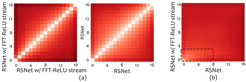
Although our FFT-ReLU stream can learn global context, multi-layer Res FFT-ReLU Block is necessary. Multi-layer can be considered as progressively deblurring the output of the previous layers. Adding FFT-ReLU stream in the first 8 layers and the last 8 layers in RSNet obtain different deblurring results (29.69 vs. 30.01), as shown in Table 6. If adding FFT-ReLU stream in the lower layers, the lack of semantic information will make the learned global information less meaningful. Besides, we show Canonical Correlation Analysis (CCA) similarities in Fig. 10 (a) between layers of features inside RSNet w/ FFT-ReLU stream, and RSNet. We can see the similarity scores between low and high layers inside RSNet w/ FFT-ReLU stream are very small, which are smaller than those in RSNet. It is also interesting to observe relatively high similarity scores between lower layers of RSNet w/ FFT-ReLU stream vs. lower and middle layers of RSNet, as pointed out in Fig. 10 (b).

Figure 11: Visualizations of the preferred inputs for different location units on the final output layer for RSNet, RSNet w/ FFT-ReLU Stream, and RSNet w/ simple-FFT-ReLU stream (gray in Table 1 in the main paper).

Figure 12: Visualizations of restored image by MIMO-UNet, FMIMO-UNet and the FFT of their difference. Sharp-Blur denotes we directly subtract Blur from Sharp images, and show one channel (Green channel). The same applies for others. $|\mathcal{F}(\cdot)|$ denotes the log of the magnitudes of 2-dimensional discrete Fourier transform, where the log operation is taking for visualization purpose.

Figure 13: Failure cases in NAFNet on RealBlur dataset.

Other Details for Visualizing Neurons

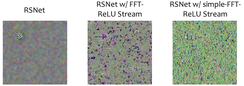
We provide some details for Visualizations of Neurons in Sec. 5.2 in the main paper. For training details, we follow the default setting (Ozbulak 2019), which includes the maximum iterations (150), optimizer (SGD), initial learning rate (6), weight decay (0.0001), and the Gaussian filter which is applied every 4 iterations. We also visualize the neuron in the output layer of different networks, including RSNet w/ simple-FFT-ReLU. For the output layer, we adopt a slightly different strategy. I.e., instead of maximizing a selected neuron, we first apply Sobel filter on the output image to obtain the edge map of the image, then we learn the best input image by maximizing the neuron on location $[\frac{1}{4}H,\frac{1}{4}W]$ on the obtained edge map. We propose to visualize the output neuron after applying a Sobel filter, because the ability of maximizing an edge point is related to the ability of image deblurring. Visualizations of the preferred inputs for different location units on the final output layer are shown in Fig. 11. It is easy to see that RSNet can only learn local context, while the other two networks have the ability to capture global context.

Visualizations of MIMO-UNet w/ and w/o Res FFT-ReLU Block

We denote the MIMO-UNet with our proposed Res FFT-ReLU Block as FMIMO-UNet. Since end-to-end image deblurring architecture learns the discrepancy between blur and sharp image pairs, given a deblurring architecture, it is intuitive to visualize the difference between the restored sharp image with the ground-truth sharp image. This difference indicates how far to go for the model to restore an ideal sharp image. We also take the FFT of the difference, as shown in Fig. 12. Compared with MIMO-UNet, by using our Res FFT-ReLU Block, FMIMO-UNet can compensate more frequency information (see $|\mathcal{F}(\text{FMIMO}-\text{MIMO})|$, and comparisons between $|\mathcal{F}(\text{Sharp}-\text{FMIMO})|$ and $|\mathcal{F}(\text{Sharp}-\text{MIMO})|$).

Table 7: Parameters, FLOPs and runtime (average testing time per image in GoPro dataset on a NVIDIA 3090 GPU) comparison. ${\ddagger}$ means testing an image for 4 times by test time augmentation.

Model	PSNR	Params.	FLOPs	Runtime
		(M)	(G)	(s)
DMPHN (Zhang et al. 2019a)	31.20	21.7	-	0.307
DBGAN (Zhang et al. 2020)	31.10	11.6	759.85	1.298
MPRNet (Zamir et al. 2021)	32.66	20.1	777.01	1.002
MIMO-UNet (Cho et al. 2021)	31.37	6.8	67.17	0.153
MIMO-UNet+	32.45	16.1	154.41	0.309
MIMO-UNet++	32.68	16.1${\ddagger}$	617.63	1.185
SDWNet (Zou et al. 2021)	31.36	7.2	189.68	0.533
UFormer (Wang et al. 2022)	33.06	50.9	89.46	0.442
Restormer (Zamir et al. 2022)	32.92	26.1	141.00	1.14
NAFNet32 (Chen et al. 2022)	32.85	17.1	16.00	0.132
NAFNet64 (Chen et al. 2022)	33.69	65.0	63.50	0.329
FMIMO-UNet-small	32.52	4.4	44.60	0.244
FMIMO-UNet	33.08	8.2	80.21	0.339
FMIMO-UNet+	33.52	19.5	187.04	0.948
FNAFNet32	33.12	17.8	23.10	0.185
FNAFNet64	33.85	68.0	72.40	0.366

Evaluation of FMIMO-UNet and FNAFNet

Detailed Analysis for Evaluation of FMIMO-UNet and FNAFNet

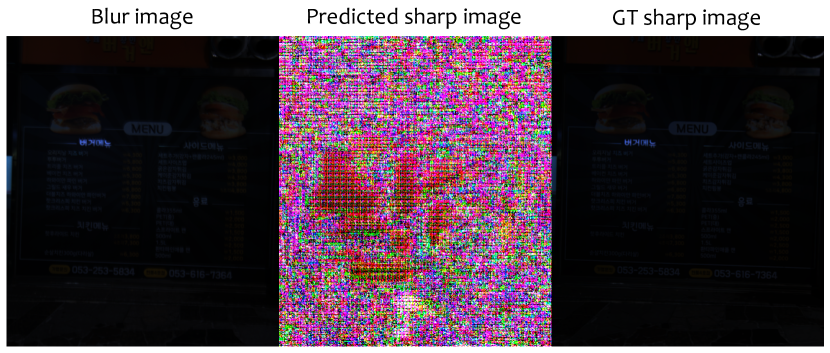
The results of FMIMO-UNet-small, FMIMO-UNet, and FMIMO-UNet+ are reported after cropping the input image to the training size of 256 with an overlap size of 32, i.e., sliding window strategy with window size 256 and stride 224. This further improves the performance for FMIMO-UNet from 32.71 dB to 33.08 dB. As shown in Table 5 in the main paper, our FMIMO-UNet-small outperforms MIMO-UNet by 0.79 dB PSNR with 2.4M less parameters (see Table 7). As mentioned above, because of our limited computation resource, for FNAFNet32, we add Res FFT-ReLU block to the first three encoder blocks and their skip connected decoder blocks. For FNAFNet64, we only add Res FFT-ReLU block to the first encoder block and its skip connected decoder block. We set the batch size to 32 for both FNAFNet32 and FNAFNet64. But for NAFNet64, the batch size was set as 64 in the paper (Chen et al. 2022). FNAFNet32 outperforms NAFNet32 by 0.27 dB and FNAFNet64 outperforms NAFNet64 by 0.16 dB. We do not report the results on NAFNet64/FNAFNet64 for RealBlur dataset, because some predicted sharp images look weird for NAFNet64, as shown in Fig. 13. This may due to the reason that the model cannot fit the distribution of the sharp image.

Parameters, FLOPs and Runtime Comparison

We compare parameters, FLOPs and runtime of our FMIMO-UNet and FNAFNet with the state-of-the-arts (see Table 7). FLOPs number is calculated using ptflops with the input size of 256$\times$256 (Zou et al. 2021). Runtime is measured by using the released test code of each method to run the entire GoPro (Nah, Kim, and Lee 2017) testing dataset, and obtaining the average runtime (second) per image on our environment with one NVidia 3090 GPU. FMIMO-UNet+ takes much less FLOPs than MIMO-UNet++ and MPRNet.

Qualitative Comparisons of FMIMO-UNet with Other Competitors

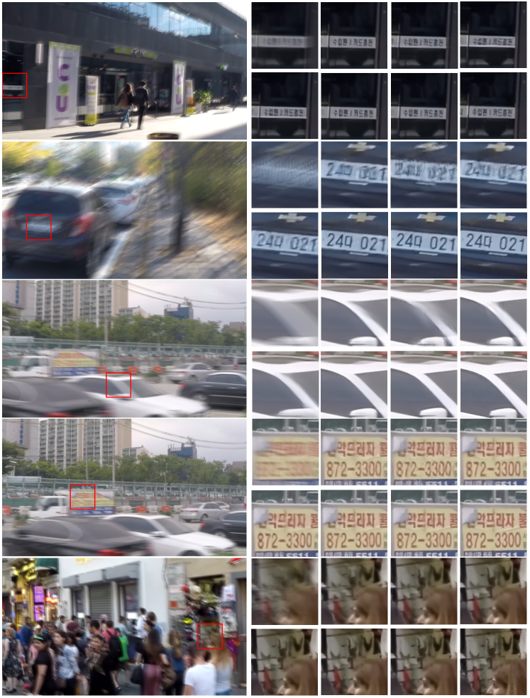
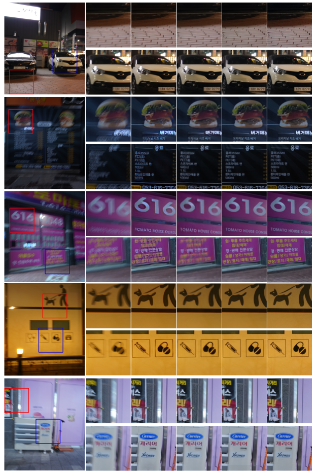
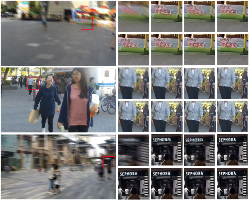
Some of the predicted sharp images from the GoPro, HIDE, and RealBlur datasets are shown in Fig. 14, Fig. 16 Fig. 15, respectively. Results from competitors are tested by using their released models. FMIMO-UNet is more successful in deblurring local details and structures compared with others.

Figure 14: Examples on the GoPro test dataset. The original blur image and the zoom-in patches are shown. From left-top to right-bottom are blurry image, results obtained through, MIMO-UNet+ (Cho et al. 2021), HINet (Chen et al. 2021), MPRNet (Zamir et al. 2021), Restormer (Zamir et al. 2022), FMIMO-UNet, FMIMO-UNet+, and the groundtruth sharp image.

Figure 15: Examples on RealBlur datasets. The original blur image and the zoom-in patches are shown. From left to right are blurry image, results obtained through DeblurGAN-v2 (Kupyn et al. 2019), SRN (Tao et al. 2018), FMIMO-UNet+ and the groundtruth sharp image.

Figure 16: Examples on HIDE datasets. The original blur image and the zoom-in patches are shown. From left-top to right-bottom are blurry image, results obtained through MIMO-UNet+ (Cho et al. 2021), HINet (Chen et al. 2021), MPRNet (Zamir et al. 2021), Restormer (Zamir et al. 2022), FMIMO-UNet, FMIMO-UNet+ and the groundtruth sharp image.

References

- Banham and Katsaggelos (1997) Banham, M. R.; and Katsaggelos, A. K. 1997. Digital image restoration. IEEE Signal Process. Mag., 14(2): 24–41.
- Brigham and Morrow (1967) Brigham, E. O.; and Morrow, R. E. 1967. The fast Fourier transform. IEEE Spectrum, 4(12): 63–70.
- Chakrabarti, Zickler, and Freeman (2010) Chakrabarti, A.; Zickler, T. E.; and Freeman, W. T. 2010. Analyzing spatially-varying blur. In Proc. CVPR.
- Chen et al. (2022) Chen, L.; Chu, X.; Zhang, X.; and Sun, J. 2022. Simple Baselines for Image Restoration. In Proc. ECCV.
- Chen et al. (2021) Chen, L.; Lu, X.; Zhang, J.; Chu, X.; and Chen, C. 2021. HINet: Half Instance Normalization Network for Image Restoration. In Proc. CVPR Workshop.
- Chen et al. (2020) Chen, X.; Xia, J. J.; Shen, D.; Lian, C.; Wang, L.; Deng, H. H.; Fung, S. H.; Nie, D.; Thung, K.; Yap, P.; and Gateno, J. 2020. One-Shot Generative Adversarial Learning for MRI Segmentation of Craniomaxillofacial Bony Structures. IEEE Trans. Medical Imaging, 39(3): 787–796.
- Cheng et al. (2021) Cheng, S.; Wang, Y.; Huang, H.; Liu, D.; Fan, H.; and Liu, S. 2021. NBNet: Noise Basis Learning for Image Denoising With Subspace Projection. In Proc. CVPR.
- Chi, Jiang, and Mu (2020) Chi, L.; Jiang, B.; and Mu, Y. 2020. Fast Fourier Convolution. In Larochelle, H.; Ranzato, M.; Hadsell, R.; Balcan, M.; and Lin, H., eds., Proc. NeurIPS.
- Chi et al. (2019) Chi, L.; Tian, G.; Mu, Y.; Xie, L.; and Tian, Q. 2019. Fast Non-Local Neural Networks with Spectral Residual Learning. In Proc. ACM MM.
- Cho et al. (2021) Cho, S.; Ji, S.; Hong, J.; Jung, S.; and Ko, S. 2021. Rethinking Coarse-to-Fine Approach in Single Image Deblurring. In Proc. ICCV.
- Dong et al. (2016) Dong, C.; Loy, C. C.; He, K.; and Tang, X. 2016. Image Super-Resolution Using Deep Convolutional Networks. IEEE Trans. Pattern Anal. Mach. Intell., 38(2): 295–307.
- Gao et al. (2019) Gao, H.; Tao, X.; Shen, X.; and Jia, J. 2019. Dynamic Scene Deblurring With Parameter Selective Sharing and Nested Skip Connections. In Proc. CVPR.
- Guo et al. (2020) Guo, Y.; Chen, J.; Wang, J.; Chen, Q.; Cao, J.; Deng, Z.; Xu, Y.; and Tan, M. 2020. Closed-Loop Matters: Dual Regression Networks for Single Image Super-Resolution. In Proc. CVPR.
- He et al. (2016) He, K.; Zhang, X.; Ren, S.; and Sun, J. 2016. Deep Residual Learning for Image Recognition. In Proc. CVPR.
- Hu et al. (2014) Hu, Z.; Cho, S.; Wang, J.; and Yang, M. 2014. Deblurring Low-Light Images with Light Streaks. In Proc. CVPR.
- Jiang et al. (2020) Jiang, K.; Wang, Z.; Yi, P.; Chen, C.; Huang, B.; Luo, Y.; Ma, J.; and Jiang, J. 2020. Multi-Scale Progressive Fusion Network for Single Image Deraining. In Proc. CVPR.
- Kingma and Ba (2015) Kingma, D. P.; and Ba, J. 2015. Adam: A Method for Stochastic Optimization. In Bengio, Y.; and LeCun, Y., eds., Proc. ICLR.
- Kupyn et al. (2018) Kupyn, O.; Budzan, V.; Mykhailych, M.; Mishkin, D.; and Matas, J. 2018. DeblurGAN: Blind Motion Deblurring Using Conditional Adversarial Networks. In Proc. CVPR.
- Kupyn et al. (2019) Kupyn, O.; Martyniuk, T.; Wu, J.; and Wang, Z. 2019. DeblurGAN-v2: Deblurring (Orders-of-Magnitude) Faster and Better. In Proc. ICCV.
- Liang et al. (2021) Liang, J.; Cao, J.; Sun, G.; Zhang, K.; Gool, L. V.; and Timofte, R. 2021. SwinIR: Image Restoration Using Swin Transformer. In Proc. ICCV Workshop.
- Loshchilov and Hutter (2017) Loshchilov, I.; and Hutter, F. 2017. SGDR: Stochastic Gradient Descent with Warm Restarts. In Proc. ICLR.
- Mei, Fan, and Zhou (2021) Mei, Y.; Fan, Y.; and Zhou, Y. 2021. Image Super-Resolution With Non-Local Sparse Attention. In Proc. CVPR.
- Nah, Kim, and Lee (2017) Nah, S.; Kim, T. H.; and Lee, K. M. 2017. Deep Multi-scale Convolutional Neural Network for Dynamic Scene Deblurring. In Proc. CVPR.
- Nah et al. (2021) Nah, S.; Son, S.; Lee, S.; Timofte, R.; and Lee, K. M. 2021. NTIRE 2021 Challenge on Image Deblurring. In Proc. CVPR Workshop.
- Ozbulak (2019) Ozbulak, U. 2019. PyTorch CNN Visualizations. https://github.com/utkuozbulak/pytorch-cnn-visualizations.
- Pan et al. (2016) Pan, J.; Sun, D.; Pfister, H.; and Yang, M. 2016. Blind Image Deblurring Using Dark Channel Prior. In Proc. CVPR.
- Pan et al. (2019) Pan, L.; Hartley, R. I.; Liu, M.; and Dai, Y. 2019. Phase-Only Image Based Kernel Estimation for Single Image Blind Deblurring. In Proc. CVPR.
- Park et al. (2020) Park, D.; Kang, D. U.; Kim, J.; and Chun, S. Y. 2020. Multi-Temporal Recurrent Neural Networks for Progressive Non-uniform Single Image Deblurring with Incremental Temporal Training. In Proc. ECCV.
- Purohit et al. (2021) Purohit, K.; Suin, M.; Rajagopalan, A. N.; and Boddeti, V. N. 2021. Spatially-Adaptive Image Restoration using Distortion-Guided Networks. In Proc. ICCV.
- Raghu et al. (2021) Raghu, M.; Unterthiner, T.; Kornblith, S.; Zhang, C.; and Dosovitskiy, A. 2021. Do Vision Transformers See Like Convolutional Neural Networks? In Proc. NeurIPS.
- Rao et al. (2021) Rao, Y.; Zhao, W.; Zhu, Z.; Lu, J.; and Zhou, J. 2021. Global Filter Networks for Image Classification. In Proc. NeurIPS.
- Rim et al. (2020) Rim, J.; Lee, H.; Won, J.; and Cho, S. 2020. Real-World Blur Dataset for Learning and Benchmarking Deblurring Algorithms. In Vedaldi, A.; Bischof, H.; Brox, T.; and Frahm, J., eds., Proc. ECCV.
- Rippel, Snoek, and Adams (2015) Rippel, O.; Snoek, J.; and Adams, R. P. 2015. Spectral Representations for Convolutional Neural Networks. In Proc. NeurIPS.
- Shen et al. (2019) Shen, Z.; Wang, W.; Lu, X.; Shen, J.; Ling, H.; Xu, T.; and Shao, L. 2019. Human-Aware Motion Deblurring. In Proc. ICCV.
- Suin, Purohit, and Rajagopalan (2020) Suin, M.; Purohit, K.; and Rajagopalan, A. N. 2020. Spatially-Attentive Patch-Hierarchical Network for Adaptive Motion Deblurring. In Proc. CVPR.
- Sun et al. (2015) Sun, J.; Cao, W.; Xu, Z.; and Ponce, J. 2015. Learning a convolutional neural network for non-uniform motion blur removal. In Proc. CVPR.
- Suvorov et al. (2022) Suvorov, R.; Logacheva, E.; Mashikhin, A.; Remizova, A.; Ashukha, A.; Silvestrov, A.; Kong, N.; Goka, H.; Park, K.; and Lempitsky, V. 2022. Resolution-robust Large Mask Inpainting with Fourier Convolutions. In Proc. WACV.
- Tao et al. (2018) Tao, X.; Gao, H.; Shen, X.; Wang, J.; and Jia, J. 2018. Scale-Recurrent Network for Deep Image Deblurring. In Proc. CVPR.
- Tu et al. (2022) Tu, Z.; Talebi, H.; Zhang, H.; Yang, F.; Milanfar, P.; Bovik, A.; and Li, Y. 2022. MAXIM: Multi-Axis MLP for Image Processing. In Proc. CVPR.
- Wang et al. (2022) Wang, Z.; Cun, X.; Bao, J.; and Liu, J. 2022. Uformer: A General U-Shaped Transformer for Image Restoration. In Proc. CVPR.
- Xu, Zheng, and Jia (2013) Xu, L.; Zheng, S.; and Jia, J. 2013. Unnatural L0 Sparse Representation for Natural Image Deblurring. In Proc. CVPR.
- Yang and Soatto (2020) Yang, Y.; and Soatto, S. 2020. FDA: Fourier Domain Adaptation for Semantic Segmentation. In Proc. CVPR.
- Yosinski et al. (2015) Yosinski, J.; Clune, J.; Nguyen, A. M.; Fuchs, T. J.; and Lipson, H. 2015. Understanding Neural Networks Through Deep Visualization. CoRR, abs/1506.06579.
- Yuan, Su, and Ma (2020) Yuan, Y.; Su, W.; and Ma, D. 2020. Efficient Dynamic Scene Deblurring Using Spatially Variant Deconvolution Network With Optical Flow Guided Training. In Proc. CVPR.
- Zamir et al. (2022) Zamir, S. W.; Arora, A.; Khan, S. H.; Hayat, M.; Khan, F. S.; and Yang, M. 2022. Restormer: Efficient Transformer for High-Resolution Image Restoration. In Proc. CVPR.
- Zamir et al. (2020) Zamir, S. W.; Arora, A.; Khan, S. H.; Hayat, M.; Khan, F. S.; Yang, M.; and Shao, L. 2020. Learning Enriched Features for Real Image Restoration and Enhancement. In Proc. ECCV.
- Zamir et al. (2021) Zamir, S. W.; Arora, A.; Khan, S. H.; Hayat, M.; Khan, F. S.; Yang, M.; and Shao, L. 2021. Multi-Stage Progressive Image Restoration. In Proc. CVPR.
- Zhang et al. (2019a) Zhang, H.; Dai, Y.; Li, H.; and Koniusz, P. 2019a. Deep Stacked Hierarchical Multi-Patch Network for Image Deblurring. In Proc. CVPR.
- Zhang et al. (2019b) Zhang, H.; Dai, Y.; Li, H.; and Koniusz, P. 2019b. Deep Stacked Hierarchical Multi-patch Network for Image Deblurring. In Proc. CVPR.
- Zhang et al. (2018a) Zhang, J.; Pan, J.; Ren, J. S. J.; Song, Y.; Bao, L.; Lau, R. W. H.; and Yang, M. 2018a. Dynamic Scene Deblurring Using Spatially Variant Recurrent Neural Networks. In Proc. CVPR.
- Zhang et al. (2020) Zhang, K.; Luo, W.; Zhong, Y.; Ma, L.; Stenger, B.; Liu, W.; and Li, H. 2020. Deblurring by Realistic Blurring. In Proc. CVPR.
- Zhang et al. (2018b) Zhang, Y.; Tian, Y.; Kong, Y.; Zhong, B.; and Fu, Y. 2018b. Residual Dense Network for Image Super-Resolution. In Proc. CVPR.
- Zhong et al. (2018) Zhong, Z.; Shen, T.; Yang, Y.; Lin, Z.; and Zhang, C. 2018. Joint Sub-bands Learning with Clique Structures for Wavelet Domain Super-Resolution. In Proc. NeurIPS.
- Zou et al. (2021) Zou, W.; Jiang, M.; Zhang, Y.; Chen, L.; Lu, Z.; and Wu, Y. 2021. SDWNet: A Straight Dilated Network with Wavelet Transformation for Image Deblurring. In Proc. ICCV Workshop.