Identifying Axion Insulator by Quantized Magnetoelectric Effect in Antiferromagnetic ${\mathrm{MnBi}}_{2}{\mathrm{Te}}_{4}$ Tunnel Junction

Abstract

Intrinsic magnetic topological insulator ${\mathrm{MnBi}}_{2}{\mathrm{Te}}_{4}$ is believed to be an axion insulator in its antiferromagnetic ground state. However, direct identification of axion insulators remains experimentally elusive because the observed vanishing Hall resistance, while indicating the onset of the axion field, is inadequate to distinguish the system from a trivial normal insulator. Using numerical Green’s functions, we theoretically demonstrate the quantized magnetoelectric current in a tunnel junction of atomically thin ${\mathrm{MnBi}}_{2}{\mathrm{Te}}_{4}$ sandwiched between two contacts, which is a smoking-gun signal that unambiguously confirms antiferromagnetic ${\mathrm{MnBi}}_{2}{\mathrm{Te}}_{4}$ to be an axion insulator. Our predictions can be verified directly by experiments.

Recently, topological insulators with intrinsic magnetism becomes a new frontier dubbed intrinsic magnetic topological insulators (MTIs), where the time reversal symmetry is broken by the spontaneous magnetic ordering rather than magnetic disorders [1, 2, 3, 4, 5, 6], holding great potential for the realization of high temperature topological materials. Since the topological phases of intrinsic MTIs are highly mingled with the magnetic states, manipulating the magnetic ordering through external magnetic fields, temperature or thickness will simultaneously tune the correlated topological states [7, 8]. For example, depending on the magnetic states, ${\mathrm{MnBi}}_{2}{\mathrm{Te}}_{4}$ (MBT) can exhibit versatile topological phases such as topological insulator [9], (high Chern number) Chern insulator [2, 10], quantum spin Hall insulator and Weyl semimetal [7], and in particular, axion insulator [11].

Unlike other topological phases characterized by the first Chern number [12, 13], an axion insulator is in a higher order topological phase characterized by the symmetry protected axion field $\theta=\pi$ [14, 15, 16, 17], which can manifest as the quantized topological magnetoelectric (TME) effect [18, 19, 20] and other striking transport phenomena [21, 22, 23, 24, 25]. However, because the first Chern number of an axion insulator vanishes identically, the ensuing transport effect on a Hall bar device exhibits a vanishing Hall resistance accompanied by a large longitudinal resistance, which is just similar to a normal insulator. This property makes it rather elusive to properly distinguish axion insulators from normal insulators by transport experiments [11]. Therefore, to confirm the existence of axion insulator, a viable experimental scheme without ambiguity is needed.

In this Letter, we propose an axion insulator tunnel junction consisting of a few-layer MBT sandwiched between two metallic contacts as an experimental setup to unambiguously identify axion insulators through the quantized TME. We first show that a perpendicular magnetic field can induce a surface charge polarization that is physically related to the layer-resolved Chern numbers and the quantized axion field $\theta=\pi$. When the magnetic field adiabatically varies with time (i.e., with a frequency far less than the insulating gap), the surface charge polarization becomes time-dependent and will generate an AC charge current through the tunnel junction. We use time-dependent non-equilibrium Green’s function to quantity the detectable AC current driven by a harmonic magnetic field, which agrees remarkably well with the time derivative of the induced charge polarization, thus strengthening the validity and reliability of our proposed scheme to identify axion insulators. Since archetypal materials parameters have been adopted in the modeling, we anticipate our theory to be able to inspire and guide experiments in the perceivable future.

Low energy effective Hamiltonian.— MBT is a van der Waals magnet consisting of Te-Bi-Te-Mn-Te-Bi-Te septuple layers (SLs) arranged on a triangle lattice with parallel intralayer ferromagnetic order while adjacent SLs are coupled antiferromagnetically. Under the basis $\begin{bmatrix}\lvert p_{z}^{+},\uparrow\rangle,&\lvert p_{z}^{-},\uparrow\rangle,&\lvert p_{z}^{+},\downarrow\rangle,&\lvert p_{z}^{-},\downarrow\rangle\end{bmatrix}^{T}$ with $\lvert p_{z}^{+(-)},\sigma\rangle$ the spin-$\sigma$ orbital of Bi (Te), the low energy Hamiltonian for a layered MBT can be written as [26, 27, 4]

$$\mathcal{H}=\sum_{a=0}^{3}d_{a}(\bm{k})\Gamma_{a}+\Delta\sum_{i}\bm{m}_{i}\cdot\bm{\sigma}\otimes\tau_{0}.$$ (1)

Here, the first term is an effective Hamiltonian for a three dimensional topological insulator, where $d_{0}(\bm{k})=M_{0}-B_{1}k_{z}^{2}-B_{2}(k_{x}^{2}+k_{y}^{2})$, $d_{1}(\bm{k})=A_{2}k_{x}$, $d_{2}(\bm{k})=A_{2}k_{y}$, $d_{3}(\bm{k})=A_{1}k_{z}$ with $A_{1(2)}$, $B_{1(2)}$, $M_{0}$ being system parameters and the lattice momentum $\bm{k}=\begin{pmatrix}k_{x},&k_{y},&k_{z}\end{pmatrix}$. $\Gamma_{0}=\sigma_{0}\otimes\tau_{3}$ and $\Gamma_{a}=\sigma_{a}\otimes\tau_{1}$ ($a=1,2,3$) where $\sigma_{a}$ and $\tau_{a}$ are Pauli matrices acting on the spin and orbital spaces, respectively. The second term describes the exchange interaction between topological electrons and magnetic ordering, where $\Delta$ is the exchange strength and $\bm{m}_{i}$ is the unit magnetization vector of the $i$-th SL [4]. Henceforth in all numerical calculations, the materials parameters are shown in Tab. 1, and temperature is set to be zero.

Table 1: Parameters adopted. $a_{0}$ is the lattice constant. $M_{0}$, $A_{1(2)}$ and $B_{1(2)}$ are based in Ref. [26]. $J$, $K$ and $M_{S}$ are chosen from Ref. [28]. $\mu_{B}$ is the Bohr magneton. The exchange gap $\Delta$ is evaluated from Refs. [29, 30].

$a_{0}$(nm)	$\Delta$(eV)	$M_{0}$(eV)	$A_{1}$(eV$\cdot$ nm)	$A_{2}$(eV$\cdot$ nm)
5	-0.05	-0.1165	0.27232	0.31964
$J$(meV)	$K$(meV)	$M_{S}$ ($\mu_{B}$)	$B_{1}$(eV$\cdot\text{nm}^{2}$)	$B_{2}$(eV$\cdot\text{nm}^{2}$)
0.68	0.21	5/2	0.119048	0.094048

Since the topological states of MBT is intertwined with the magnetic ordering, we first need to determine its magnetic configuration. In the macro-spin approximation (spatially uniform magnetization within a particular SL), the magnetic property of an $N$-SL MBT can be characterized by the free energy [31, *Mills1968Sur]

$$U=J\sum_{i=1}^{N-1}\bm{m}_{i}\cdot\bm{m}_{i+1}-\sum_{i=1}^{N}\left[\frac{K}{2}(m_{i}^{z})^{2}+M_{s}\bm{\mathcal{B}}\cdot\bm{m}_{i}\right],$$ (2)

where $J$ is the antiferromagnetic interlayer exchange interaction, $K$ is the easy-axis anisotropy, $\bm{\mathcal{B}}$ is external magnetic field, and $M_{s}$ is the saturation magnetization of each SL. The magnetization vector is parameterized as $\bm{m}_{i}=\{\sin\theta_{i}\cos\phi_{i},\sin\theta_{i}\sin\phi_{i},\cos\theta_{i}\}$ with $\theta_{i}$ ($\phi_{i}$) the polar (azimuthal) angle. Without losing generality, we assume that $\bm{\mathcal{B}}$ is applied along $z$ direction and $\bm{m}_{i}$ rotates only in the $xz$ plane. We obtain the equilibrium magnetic configuration by minimizing the free energy $U$ using the steepest descent method [33, *Rossler2006Spin], which is detailed in the supplementary materials (SM) [35].

Figure. 1(a) shows the total magnetization as a function of the applied magnetic field for a six-SL MBT, where we identify the spin-flop critical points at around $\mathcal{B}_{c}^{\pm}\approx\pm 3$T, beyond which the Zeeman energy overcomes the exchange and anisotropy interactions and induces non-collinear spin configurations until the system is fully polarized into a ferromagnetic state at above $10$T (see Fig. S1 in the SI). Such distinct magnetic evolution is in quantitative agreement with experiments [2, 11]. The complicated spin configurations in the intermediate spin-flop phases are discussed in the SM [35].

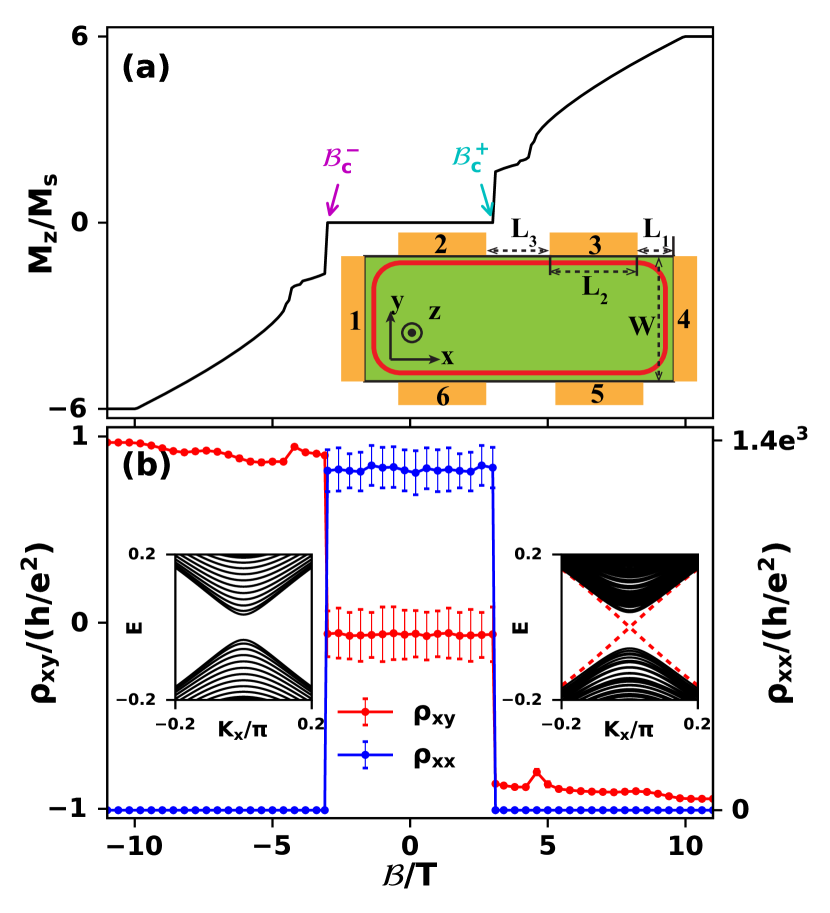
Figure 1: (a) Total magnetization as a function of magnetic field for a 6-SL MBT. Inset: schematics of a Hall bar device where the metallic leads are shaded orange and the MBT is colored green. The red curve marks the edge channel when the MBT becomes a Chern insulator (i.e., when $|\mathcal{B}|>|\mathcal{B}_{c}^{\pm}|$). (b) Longitudinal resistivity $\rho_{xx}$ and Hall resistivity $\rho_{xy}$ as functions of magnetic field. The data is obtained on a Hall bar of size $L_{1}\times L_{2}\times L_{3}\times W=5\times 50\times 30\times 50$ with a disorder strength $D=0.1$ eV (comparable to the magnetic exchange gap) after averaging over 160 computations. Insets: band structures along the $x$ direction for a 6-SL MBT in its antiferromagnetic (left) and ferromagnetic (right) states.

In-plane transport properties on a Hall bar.— To study the electronic transport, we first discretize the continuum Hamiltonian Eq. (1) on a cubic lattice ($a_{0}=5$nm) invoking the $k\cdot p$ perturbation. Then, under a Hall bar device geometry as illustrated in the inset of Fig. 1(a), we calculate the Hall resistivity $\rho_{xy}$ and the longitudinal resistivity $\rho_{xx}$ using the Landauer-Büttiker formula [35, 36]. To incorporate fluctuations, we also add a disorder potential $\mathcal{H}_{D}=V(\bm{r})s_{z}\otimes\sigma_{0}$ to the lattice Hamiltonian, where $V(\bm{r})$ is uniformly distributed within $[-D/2,\ D/2]$ with $D$ being the disorder strength. The Fermi level is zero as we do not consider doping or gating.

For a six-SL MBT device reflecting real experimental setup [11], we obtain $\rho_{xx}$ and $\rho_{xy}$ by averaging 160 repeated calculations, which are plotted as functions of magnetic field $\mathcal{B}$ (along $z$) in Fig. 1(b). The results show a topological phase transition from a normal insulator (indistinguishable from an axion insulator) with a vanishing Chern number $\mathcal{C}=0$ at low magnetic fields into a quantum anomalous Hall insulator with $\mathcal{C}=\pm 1$ at high magnetic fields. When $\lvert\mathcal{B}\rvert<\mathcal{B}_{c}^{+}$, the magnetic ground state remains antiferromagnetic with antiparallel spins on adjacent SL, and the system preserves the $\mathcal{PT}$ symmetry. Because the spin flips its sign under $\mathcal{PT}$ operation [$\mathcal{PT}$: $\mathcal{H}(\bm{k},\uparrow)\rightarrow\mathcal{H}(\bm{k},\downarrow)$], the bands must be doubly degenerate with a band gap of $\delta\approx 2\Delta$ at $k_{x}=0$, as shown in the left inset in Fig. 1(b). Consequently, we obtain $\mathcal{C}=0$, hence a vanishing Hall resistivity and a large longitudinal resistivity akin to a normal insulator. While ARPES experiments showed controversial results on the band gap in MBT [29, 37], transport measurements strongly support the existence of large gaps in both the antiferromagnetic and ferromagnetic states of MBT [11, 2, 10] by confirming the insulating behavior in longitudinal transport, even though this insulating gap cannot tell axion insulators from normal insulators.

When $\lvert\mathcal{B}\rvert$ exceeds $\mathcal{B}_{c}^{+}$, however, the magnetic moments undergo a spin-flop transition which breaks the time reversal symmetry for electrons. Correspondingly, the topological Chern number becomes $\mathcal{C}=-\text{sgn}(\mathcal{B})$, leading to a quantized Hall resistivity $\rho_{xy}=h/(\mathcal{C}e^{2})$ and a vanishing longitudinal resistivity $\rho_{xx}=0$ [12]. The deviations of $\rho_{xy}$ around integer values are ascribed to the finite size effect, which can be suppressed by enlarging the system size. The in-plane resistivities shown in Fig. 1 agree quantitatively with experimental observations [Cai2022Electric, 11] widely regarded as evidences for axion insulator. Nevertheless, the topological phase transition taking place here is inadequate to determine an axion insulator because the $\mathcal{C}=0$ phase appearing at small fields by itself is indistinguishable from a normal insulator.

Surface charge polarization and layer-resolved Chern numbers.— A defining feature of axion insulator is the topological TME enabled by the quantized $\theta$-field, which, unlike the Chern number $\mathcal{C}$, can uniquely characterize the axion insulator phase. On the one hand, a magnetic field $\bm{B}$ below the spin-flop threshold will induce a quantized charge polarization $\bm{P}=e^{2}\theta\bm{B}/(2\pi h)$ [14], which is intimately related to the layer-resolved Chern numbers. If the applied $\bm{B}$ field is time dependent, a charge current proportional to $d\bm{P}/dt$ will be generated, enabling a directly detectable signal to be discussed later. On the other hand, the TME also manifests as the magnetization induced by an electric field [39]. However, the TME coefficient quantized by $\theta$ is typically two orders of magnitude smaller than that of ordinary magnetoelectric materials [40]. Therefore, the TME is more amenable to transport measurement as the sensitivity of detecting current is extremely high. Nonetheless, as a consistency check, we also calculated the tiny magnetization induced by an electric field, which indeed turns out to be quantized by the $\theta$ field (see the SM [35]).

To calculate $\bm{P}$, we consider a slab of thickness $L_{z}$ and widths $L_{x}=L_{y}$ with open boundary conditions and assume that a static magnetic field $\bm{B}=(0,0,B)$ is applied along the $z$-direction, which amounts to a magnetic flux of $\Phi_{0}=Ba_{0}^{2}$ per unit cell. Using the equilibrium Green’s function method [35], we obtain the charge distribution $Q(\bm{r})=-e\langle\hat{n}(\bm{r})\rangle$ where $-e$ is the electron charge and $\hat{n}(\bm{r})$ is the electron density operator. Figure 2 (blue dots) plots the charge distribution among each SL, $Q_{z}=\sum_{x,y}Q(\bm{r})$, with respect to an averaged background charge $\overline{Q(\bm{r})}=\sum_{x,y,z}Q(\bm{r})/L_{z}$ which compensates the positive ions in the lattice. Since $Q(\bm{r})$ is an odd function of $z$, as shown in Fig. 2, there is indeed a finite charge polarization $\bm{P}=\int dV\bm{r}Q(\bm{r})$. As will be shown later, only surface charges contribute to the detectable current, thus only the surface charge polarization $P_{z}=[Q(L_{z}/2)-Q(-L_{z}/2)]/2-\overline{Q(\bm{r})}$ is relevant to our discussion. Ideally, the surface charge polarization $P_{z}$ should be very close the total polarization $P$, but finite-size effects can bring about deviations. Fortunately, we find that the finite-size effects are well suppressed by increasing the thickness $L_{z}$. It turns out that $P_{z}(L_{z}=6,8,10)=0.91,0.97,0.99$ ($e^{2}\Phi/2h$) with $\Phi=L_{x}L_{y}\Phi_{0}$ being the total magnetic flux penetrating the slab, rapidly approaching the quantized value determined by the axion field $\theta=\pi$.

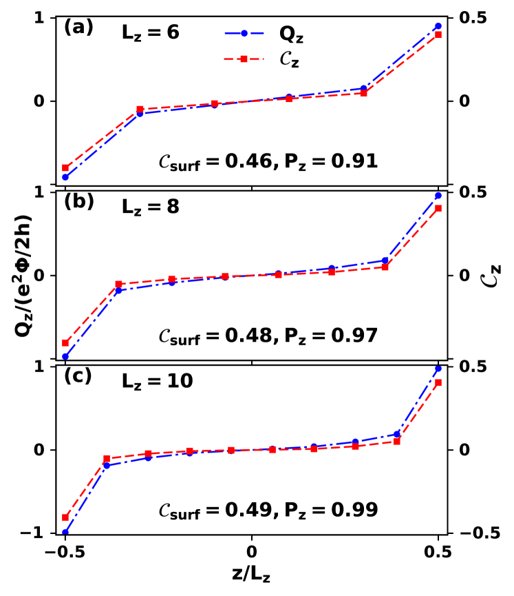
Figure 2: Charge distribution among each SL relative to the background average $Q_{z}-\overline{Q(\bm{r})}$ (blue dots) and layer-resolved Chern numbers $\mathcal{C}_{z}$ (red squres) for MBT of thickness (a) $L_{z}=6$, (b) $L_{z}=8$, and (c) $L_{z}=10$ on a slab of size $L_{x}\times L_{y}\times L_{z}$ with $L_{x}=L_{y}=40$. Here, the magnetic flux per unit cell is $\Phi_{0}=0.05h/2e$ and the total magnetic flux is $\Phi=L_{x}L_{y}\Phi_{0}$, which corresponds to a magnetic field of $B=2\text{T}$ smaller than the spin-flop threshold $\mathcal{B}_{c}\approx 3.0\text{T}$ ($a_{0}=5$nm).

We now turn to the layer-resolved Chern numbers $\mathcal{C}_{z}$ which reflect the relative contribution to the system topology by different SLs. To this end, we adopt periodic boundary conditions in the lateral dimensions under the same slab geometry used above. While the layer-resolved Chern numbers can be straightforwardly obtained by projecting the wavefunctions onto each SL [35] in a clean system, here we resort to the non-commutative approach which is able to incorporate disorders [41, *Prodan2012Quantum]: $\mathcal{C}_{z}=-2\pi i\text{Tr}\left\{\hat{P}\left[[\hat{x},\ \hat{P}],\ [\hat{y},\ \hat{P}]\right]\hat{P}_{z}\right\}$, where $\hat{x}$ ($\hat{y}$) is the position operator, $\hat{P}$ is the projector onto the occupied bands, $\hat{P}_{z}\equiv\lvert\psi_{z}\rangle\langle\psi_{z}\rvert$ is the projector onto the $z$-th SL, $[\cdots]$ is the commutator and Tr denotes the trace. In the presence of $\mathcal{PT}$ symmetry, $\hat{P}_{z}$ flips sign on opposite surfaces because $\hat{P}_{-z}=|\psi_{-z}\rangle\langle\psi_{-z}|=\mathcal{PT}|\psi_{z}\rangle\langle\psi_{z}|\mathcal{PT}=(\mathcal{PT})^{2}|\psi_{z}\rangle\langle\psi_{z}|=-|\psi_{z}\rangle\langle\psi_{z}|=-\hat{P}_{z}$, ensuring that the layer-resolved Chern numbers are odd in $z/L_{z}$.

Figure 2 shows the layer-resolved Chern numbers $\mathcal{C}_{z}$ with three different thicknesses $L_{z}=6,8,10$ (red squares), which agrees remarkably well with the charge distribution $Q_{z}$. Even in the presence of disorders, we find that $\mathcal{C}_{z}$ and $Q_{z}$ are very robust (See SM [35]), suggesting that they are topologically protected properties intrinsic to the axion insulator. Correspondingly, the surface Chern number $\mathcal{C}_{surf}^{L_{z}}=\sum_{z=-L_{z}/2}^{0}\mathcal{C}_{z}$ is almost half quantized: $\mathcal{C}_{surf}^{6}=0.46$, $\mathcal{C}_{surf}^{8}=0.48$, and $\mathcal{C}_{surf}^{10}=0.49$, indicating a distinct bulk axion field $\theta=\pi$ [43].

Charge current in MBT tunnel junction.— To detect the quantized TME in MBT using transport experiment, we need to consider a time-dependent magnetic field such that the induced surface charge polarization becomes dynamical and produces a charge current in the $z$ direction. This approach has been utilized to characterize multiferroic materials exhibiting non-quantized magnetoelectric effects [40]. To this end, we conceive an axion insulator tunnel junction (AITJ) consisting of an even-SL MBT sandwiched between two metallic contacts  as illustrated in Fig. 3(a). In the adiabatic limit, the charge polarization follows the magnetic field at any instant of time, which can be detected directly as an AC output signal from the AITJ. Since the metallic contacts are connected only to the top and bottom layers, only the surface polarization $P_{z}$ is relevant to the transport measurement.

Using the lattice Hamiltonian, we resort to the time-dependent non-equilibrium Green’s function to compute the output current in the AITJ [35]. A harmonic magnetic field $\bm{B}(t)=\hat{\bm{z}}B\sin{\omega t}$ applied to the AITJ converts to a phase $\Phi_{0}(t)=\Phi_{0}\sin{\omega t}$ for electrons, where $\Phi_{0}=Ba_{0}^{2}$ is the magnetic flux per unit cell. As a result, the effective Hamiltonian acquires a time-dependent perturbation that drives the electron motion, forming a charge current. Since the system is now periodic in time, the induced charge current can be expanded into a Fourier series as [35, 45]

$$I(t)=\sum_{n=-\infty}^{\infty}I_{n}e^{in\omega t},$$ (3)

where $I_{n}$ is $n$-th harmonic component satisfing $I_{n}=-I_{-n}^{*}$, ensuring a real current. The total current $I(t)$ includes a DC component $I_{0}$ and a series of AC components $I_{n>0}$. Truncating the Green’s function at order $n=4$ suffices to yield a converging result [35]. Figure 3(b) (solid blue curve) plots the numerical result of $I(t)$ for one period of oscillation, where the first order term $I_{n=\pm 1}$ indeed dominates all other components. The plot is offset by $I_{0}$ because this DC component is short circuited via the bias tee illustrated in Figure 3(a).

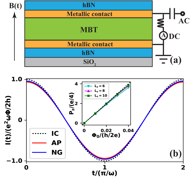
Figure 3: (a) Schematics of the proposed AITJ setup to detect the dynamical TME. The metallic leads are connected to a bias tee to separate the harmonic AC output from the DC output which is short circuited. The hexagonal boron nitride (hBN) flakes are added to avoid degradation [46], and the whole device is placed on a silicon dioxide substrate. (b) Output current $I(t)$ induced by an AC magnetic field $\hat{\bm{z}}B\sin\omega t$ calculated by the time-dependent non-equilibrium Green’s function (NG) (solid blue), the adiabatic variation of the surface charge polarization (AP) (solid red), respectively. The ideal case (IC) (dotted black) for an exactly quantized axion field $\theta=\pi$ is plotted as a reference. System size: $L_{x}=L_{y}=20$ and $L_{z}=6$. Magnetic flux per unit cell: $\Phi_{0}=0.05h/2e$. Driving frequency: $\hbar\omega=0.001\text{eV}$. Inset: surface charge polarization as a function of the magnetic flux for three different thicknesses $L_{z}=6,8,10$.

As an independent confirmation, we use the same harmonic field $\bm{B}(t)=\hat{\bm{z}}B\sin{\omega t}$ in the surface charge polarization $P_{z}$ and calculate the resulting charge current $I_{z}(t)=dP_{z}(t)/dt$ [47], assuming an adiabatic condition that $\bm{P}$ undergoes a quasi-static variation without inter-band transitions induced by the oscillating $\bm{B}(t)$ [48]. Figure 3(b) (solid red curve) plots $I_{z}(t)$ within one period of oscillation for a same MBT slab, which agrees remarkably well with the harmonic signal $I(t)$ obtained by the non-equilibrium Green’s function method. To benchmark the accuracy of our numerical results, we also plot the ideal case for an infinite system, where $I(t)=dP(t)/dt=\theta e^{2}/(2\pi h)\omega\Phi\cos\omega t$ with a strictly quantized axion field $\theta=\pi$ (dotted black curve in Fig. 3(b)). We see that our numerical results obtained both from the non-equilibrium Green’s functions and from $P_{z}(t)$ only slightly deviate from the ideal case, which demonstrates the validity and reliability of our proposal. We mention in passing that if the Fermi level is tuned into the conducting band (e.g., by gating the device [49]), the MBT will become metallic and the induced AC current will vanish.

For an MBT of size $L_{x}=L_{y}=10\rm{\mu m}$, a harmonic magnetic field of strength $B\sim 100$Gs and frequency $\omega/2\pi=1$GHz induces an output AC current $I\sim 121.54$nA, which is a conservative estimation. Since $I$ scales as $\omega BL_{x}L_{y}$, the output current can be amplified by increasing the driving frequency $\omega$, the magnetic field $B$, or the system size in the lateral dimensions. In the ideal case, the induced surface charge polarization $P_{z}$ should scale linearly with the magnetic flux per unit cell $\Phi_{0}$. To evaluate potential deviations due to finite-size effects, we plot $P_{z}$ as a function of $\Phi_{0}$ for different thicknesses against the ideal scaling in the inset of Fig. 3(b), where the finite-size effects turn out to be negligible, further confirming the validity of our calculations.

In summary, we have theoretically proposed an experimental setup to unambiguously identify antiferromagnetic MBT as an axion insulator by detecting the AC current induced by a harmonic magnetic field under the adiabatic condition. Comparing to the vanishing Hall resistance measured in previous experiments, which is inadequate to confirm the axion insulator phase, our proposed scheme provides a smoking-gun signal to identify MBT as an axion insulator.

Acknowledgments.— This work is supported by the Air Force Office of Scientific Research under grant FA9550-19-1-0307. We acknowledge helpful discussions with Chong Wang and U. K. Rößler.

References

- Tokura et al. [2019] Y. Tokura, K. Yasuda, and A. Tsukazaki, Nature Reviews Physics 1, 126 (2019).
- Deng et al. [2020] Y. Deng et al., Science 367, 895 (2020).
- Li et al. [2019a] H. Li et al., Phys. Rev. X 9, 041039 (2019a).
- Li and Cheng [2021] Y.-H. Li and R. Cheng, Phys. Rev. Lett. 126, 026601 (2021).
- Li et al. [2021] H. Li, H. Jiang, C.-Z. Chen, and X. C. Xie, Phys. Rev. Lett. 126, 156601 (2021).
- Song et al. [2021] Z.-D. Song et al., Phys. Rev. Lett. 127, 016602 (2021).
- Li et al. [2019b] J. Li, Y. Li, S. Du, Z. Wang, B.-L. Gu, S.-C. Zhang, K. He, W. Duan, and Y. Xu, Science Advances 5, eaaw5685 (2019b).
- Gu et al. [2021] M. Gu, J. Li, H. Sun, Y. Zhao, C. Liu, J. Liu, H. Lu, and Q. Liu, Nature Communications 12, 3524 (2021).
- Gong et al. [2019] Y. Gong et al., Chinese Physics Letters 36, 076801 (2019).
- Ge et al. [2020] J. Ge et al., National Science Review 7, 1280 (2020).
- Liu et al. [2020] C. Liu et al., Nature Materials 19, 522 (2020).
- Thouless et al. [1982] D. J. Thouless, M. Kohmoto, M. P. Nightingale, and M. den Nijs, Phys. Rev. Lett. 49, 405 (1982).
- Hasan and Kane [2010] M. Z. Hasan and C. L. Kane, Rev. Mod. Phys. 82, 3045 (2010).
- Qi et al. [2008] X.-L. Qi, T. L. Hughes, and S.-C. Zhang, Phys. Rev. B 78, 195424 (2008).
- Qi and Zhang [2011] X.-L. Qi and S.-C. Zhang, Rev. Mod. Phys. 83, 1057 (2011).
- Zhang et al. [2020] R.-X. Zhang, F. Wu, and S. Das Sarma, Phys. Rev. Lett. 124, 136407 (2020).
- Xu et al. [2019] Y. Xu, Z. Song, Z. Wang, H. Weng, and X. Dai, Phys. Rev. Lett. 122, 256402 (2019).
- Sekine and Nomura [2021] A. Sekine and K. Nomura, Journal of Applied Physics 129, 141101 (2021).
- Zhao and Liu [2021] Y. Zhao and Q. Liu, Applied Physics Letters 119, 060502 (2021).
- Nenno et al. [2020] D. M. Nenno, C. A. C. Garcia, J. Gooth, C. Felser, and P. Narang, Nature Reviews Physics 2, 682 (2020).
- Wu et al. [2016] L. Wu, M. Salehi, N. Koirala, J. Moon, S. Oh, and N. P. Armitage, Science 354, 1124 (2016).
- Tse and MacDonald [2010] W.-K. Tse and A. H. MacDonald, Phys. Rev. Lett. 105, 057401 (2010).
- Nomura and Nagaosa [2011] K. Nomura and N. Nagaosa, Phys. Rev. Lett. 106, 166802 (2011).
- Qi et al. [2009] X.-L. Qi, R. Li, J. Zang, and S.-C. Zhang, Science 323, 1184 (2009).
- Gao et al. [2021] A. Y. Gao et al., Nature 595, 521 (2021).
- Zhang et al. [2019] D. Zhang, M. Shi, T. Zhu, D. Xing, H. Zhang, and J. Wang, Phys. Rev. Lett. 122, 206401 (2019).
- Lian et al. [2020] B. Lian, Z. Liu, Y. Zhang, and J. Wang, Phys. Rev. Lett. 124, 126402 (2020).
- Yang et al. [2021] S. Yang et al., Phys. Rev. X 11, 011003 (2021).
- Otrokov et al. [2019] M. M. Otrokov et al., Nature 576, 416 (2019).
- Zeugner et al. [2019] A. Zeugner et al., Chemistry of Materials 31, 2795 (2019).
- Mills [1968] D. L. Mills, Phys. Rev. Lett. 20, 18 (1968).
- Mills and Saslow [1968] D. L. Mills and W. M. Saslow, Phys. Rev. 171, 488 (1968).
- Rößler and Bogdanov [2004] U. K. Rößler and A. N. Bogdanov, Phys. Rev. B 69, 094405 (2004).
- Roessler and Bogdanov [2006] U. K. Roessler and A. N. Bogdanov, arXiv e-prints , cond-mat/0605493 (2006), arXiv:cond-mat/0605493 [cond-mat.mtrl-sci] .
- [35] See the supplemental materials for more informations.
- Datta [1995] S. Datta, Electronic Transport in Mesoscopic Systems, Cambridge Studies in Semiconductor Physics and Microelectronic Engineering (Cambridge University Press, 1995).
- Shikin et al. [2020] A. M. Shikin, D. A. Estyunin, I. I. Klimovskikh, S. O. Filnov, E. F. Schwier, S. Kumar, K. Miyamoto, T. Okuda, A. Kimura, K. Kuroda, K. Yaji, S. Shin, Y. Takeda, Y. Saitoh, Z. S. Aliev, N. T. Mamedov, I. R. Amiraslanov, M. B. Babanly, M. M. Otrokov, S. V. Eremeev, and E. V. Chulkov, Scientific Reports 10, 13226 (2020).
- Cai et al. [2021] J. Cai, D. Ovchinnikov, Z. Fei, M. He, T. Song, Z. Lin, C. Wang, D. Cobden, J.-H. Chu, Y.-T. Cui, C.-Z. Chang, D. Xiao, J. Yan, and X. Xu, “Electric control of a canted-antiferromagnetic chern insulator,” (2021), arXiv:2107.04626 [cond-mat.mes-hall] .
- Pournaghavi et al. [2021] N. Pournaghavi, A. Pertsova, A. H. MacDonald, and C. M. Canali, Phys. Rev. B 104, L201102 (2021).
- Nan et al. [2008] C.-W. Nan, M. Bichurin, S. Dong, D. Viehland, and G. Srinivasan, Journal of applied physics 103, 1 (2008).
- Prodan [2011] E. Prodan, Journal of Physics A: Mathematical and Theoretical 44, 113001 (2011).
- Prodan [2012] E. Prodan, Applied Mathematics Research eXpress 2013, 176 (2012).
- Essin et al. [2009] A. M. Essin, J. E. Moore, and D. Vanderbilt, Phys. Rev. Lett. 102, 146805 (2009).
- Note [1] In artificial heterostructures involving 2D materials, graphene contacts are preferred (see, for example, Refs. [46, 49]) because it can be incorporated without the need for lattice matching.
- Li et al. [2018] Y.-H. Li, J. Song, J. Liu, H. Jiang, Q.-F. Sun, and X. C. Xie, Phys. Rev. B 97, 045423 (2018).
- Song et al. [2018] T. Song, X. Cai, M. W.-Y. Tu, X. Zhang, B. Huang, N. P. Wilson, K. L. Seyler, L. Zhu, T. Taniguchi, K. Watanabe, M. A. McGuire, D. H. Cobden, D. Xiao, W. Yao, and X. Xu, Science 360, 1214 (2018).
- Li et al. [2010] R. D. Li, J. Wang, X. L. Qi, and S. C. Zhang, Nature Physics 6, 284 (2010).
- [48] So long as the driving frequency is far less than the band gap of the MBT, we can treat the magnetic field as varying adiabatically. The driving frequency of the magnetic field is on the order of eV, which is indeed far less than the energy gap meV.
- Jiang et al. [2018] S. Jiang, J. Shan, and K. F. Mak, Nature Materials 17, 406 (2018).