Many-body localized to ergodic transitions in a system with correlated disorder

Abstract

We study the transition from a many-body localized phase to an ergodic phase in spin chain with correlated random magnetic fields. Using multiple statistical measures like gap statistics and extremal entanglement spectrum distributions, we find the phase diagram in the disorder-correlation plane, where the transition happens at progressively larger values of the correlation with increasing values of disorder. We then show that one can use the average of sample variance of magnetic fields as a single parameter which encodes the effects of the correlated disorder. The distributions and averages of various statistics collapse into a single curve as a function of this parameter. This also allows us to analytically calculate the phase diagram in the disorder-correlation plane.

Introduction: Strongly disordered interacting systems in one dimension exhibit the phenomenon of many-body localization (MBL), characterized by absence of transport and breakdown of standard equilibrium statistical mechanics mirlin ; basko . This has now been established both theoretically huse_review ; altman_review ; fabien_review and through experiments on ultra-cold atomic systems mblexpt1 ; mblexpt2 . The energy eigenstates of these systems (at finite energy density) exhibit low entanglement entropy, violate the eigenstate thermalization hypothesis (ETH) deutsch ; srednicki ; altman_review ; huse_review ; fabien_review , and show characteristic bimodal distribution of entanglement eigenvalues yang ; ent_spectrum . They also show characteristic features in the distribution of the lowest entanglement spectra abhisek_kedar . These features clearly distinguish the MBL phase from the standard ergodic phase, which follow ETH, have large entanglement entropy, and show unimodal distribution of entanglement eigenvalues. By increasing the fluctuations of the random couplings, which are the microscopic manifestation of disorder, one can tune a system from the ergodic phase to the MBL phase. This is known as the MBL-ergodic phase transition  oganesyan ; apal ; heisenberg ; xxz ; pollmann ; nicolas ; nicolas ; dimer2d ; quasiperiodic .

The theoretical models of MBL huse_review ; altman_review ; fabien_review have mostly used local Hamiltonians with random short-range couplings. These couplings are drawn independently from a distribution, leading to models with uncorrelated disorder. However, in a real experimental system, one would expect the random couplings to be correlated; e.g. in a solid state system with impurities, the disorder potential will decay with distance, leading to correlated disorder. For non-interacting systems, correlation in disorder is known to change the phenomenology of Anderson localization izrailev ; croy , with mobility edges appearing in systems that are completely localized in absence of correlations.

In this Letter, we explore the MBL-ergodic transition in a disordered spin chain in presence of correlated disorder in magnetic fields. We first construct a model of correlated disorder, where one can tune the overall scale of fluctuations and correlations in the disorder independently. This allows us to consider different scenarios ranging from weak to strong disorder with negligible to large correlations and tune between these limits using only two parameters. We track the MBL-ergodic transition in the fluctuation-correlation plane using several statistics from average value of the ratio of successive level spacings of the eigenstates to the distribution of the lowest few entanglement spectra of the eigenstates and find the corresponding phase diagram. The ergodic phase exists at all values of correlation at low disorder, while it exists only at very high correlations at strong disorder.

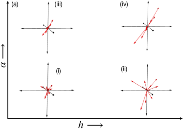
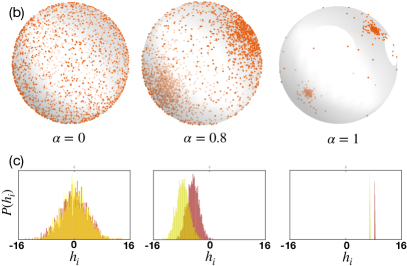
Figure 1: (a): A schematic showing how the distribution of the random coupling vectors change with $h$ and $\alpha$. Few sample vectors are shown for a $L=3$ site system in different regions of the $h-\alpha$ plane: (i) $h=1.5$, $\alpha=0.1$, (ii) $h=3.5$, $\alpha=0.1$, (iii) $h=1.5$, $\alpha=0.99$ and (iv) $h=3.5$, $\alpha=0.99$. As $h$ increases, the distribution of length of the vectors broadens, while increasing $\alpha$ narrows their angular distribution. (b): A representation of the unit vectors obtained from the random coupling vectors of the $L=3$ site system for three different values of $\alpha=0,~{}0.8,~{}1$ at fixed $h=4$. This clearly shows the evolution of the angular distribution from an uniform distribution on the unit sphere at $\alpha=0$ to a narrowly bunched distribution around the $(1,1,1)$ direction. Note that the angular distribution has finite width at $\alpha=1$ since we are looking at $L=3$. This will approach a delta function as $L\rightarrow\infty$. (c) The distribution of magnetic fields $h_{i}$, obtained from a single sample realization, for a system of $L=2000$ sites for $\alpha=0,~{}0.8,~{}1$ at fixed $h=1$. The sample distribution narrows to a delta function as $\alpha$ is increased from $0$ to $1$, showing that fields at different sites in the system are getting correlated. Distributions obtained from two different samples are plotted in the same graph. At $\alpha=0$ the distributions overlap, while the overlap decreases with increasing $\alpha$. This shows that at large $\alpha$ the inter-sample variation of $h_{i}$ is much larger than its intra-sample variation.

Increasing correlations in our model of disorder leads to less fluctuations between random couplings in a given realization. Using this idea, we define the average of sample variance as a single parameter which controls the phases and phase boundaries of the system. This is corroborated by the collapse of the gap statistics and the lowest entanglement spectrum distributions, obtained at different points in the fluctuation-correlation plane, into a single curve when the data is plotted as a function of the average sample variance. This allows us to analytically determine the phase boundary of the system. We note that the correlated disorder we consider is among the random couplings in real space, which is different from considerations of correlated randomness in Fock space  subroto ; sthitadhi1 ; sthitadhi2 . In fact, while correlated disorder in Fock space is thought to be essential for MBL phases to exist sthitadhi3 , increasing correlations in our disorder model actually favours the ergodic phase.

The model: We work with the spin-$1/2$ Heisenberg model on a one-dimensional chain of $L$ sites with nearest neighbour antiferromagnetic coupling. The spin-$1/2$ degrees of freedom also experience a random magnetic field along the $z$ direction at each site, which breaks both translation invariance and the global $SU(2)$ invariance of the underlying Heisenberg Hamiltonian. The Hamiltonian of this disordered model is given by

$$H=J\sum_{i}\sigma^{z}_{i}\sigma^{z}_{i+1}+\frac{1}{2}(\sigma^{+}_{i}\sigma^{-}_{i+1}+\sigma^{-}_{i}\sigma^{+}_{i+1})-\sum_{i}h_{i}\sigma^{z}_{i}$$ (1)

We set $J=1$ as a unit of energy. The magnetic fields $h_{i}$ are random variables drawn from a multivariate Gaussian distribution

$$P(h_{1},h_{2},..h_{L})=\frac{1}{(2\pi)^{\frac{L}{2}}\sqrt{\textrm{Det}C^{-1}}}e^{-\frac{1}{2}h_{i}C^{-1}_{ij}h_{j}}$$ (2)

where the covariance matrix $C_{ij}=\langle h_{i}h_{j}\rangle$ is given by

$$C_{ij}=h^{2}\left[\delta_{ij}+\alpha(1-\delta_{ij})\right]~{}~{}~{}0\leq\alpha\leq 1$$ (3)

The parameter $h$ denotes the standard deviation of $h_{i}$, while their cross-correlators are given by $\langle h_{j}h_{j}\rangle=h^{2}\alpha$ for $i\neq j$. It is evident that $\alpha=0$ corresponds to the case of $h_{i}$ being uncorrelated Gaussian random variables, which was studied in Ref. abhisek_kedar, . In this case, the system exhibits a MBL to ergodic phase transition at a critical disorder strength $h_{c}(0)=1.6-1.8$, depending on the statistics used to track the transition.

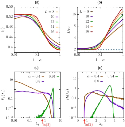
Figure 2: (a)-(b): For the Heisenberg model with random magnetic fields drawn from a Gaussian distribution with correlation $\alpha$, the average ratio of adjacent many-body gaps $\langle r\rangle$ (a) and the Kullback-Leibler parameter $D_{KL}$ (b) are plotted as function of $1-\alpha$ for different system sizes. As $\alpha$ changes from $0$ (uncorrelated disorder) to $1$ (extremely correlated disorder), the system transitions from the MBL to the ergodic phase. The value of $\langle r\rangle$ changes from its Poissonian value of $0.39$ to the Wigner-Dyson value of $0.53$. $D_{KL}$ goes to a constant value of $2$ in the ergodic limit ($\alpha=1$), and scales with system size in the MBL limit ($\alpha\rightarrow 0$). (c)-(d): The distribution of lowest two entanglement eigenvalues, $\lambda_{1}$ and $\lambda_{2}$ are plotted for $\alpha=0.4,0.8$ and $0.94$. Here the system size $L=16$ and the subsystem size $L_{A}=8$. In the MBL phase ($\alpha=0.4$), $P_{1}(\lambda_{1})$ shows a decreasing power law up to $\ln(2)$ and $P_{2}(\lambda_{2})$ develops a finite value at $\ln(2)$. In the ergodic phase ($\alpha=0.94$), $P_{1}(\lambda_{1})$ goes to $0$ at $\lambda_{1}=0$, while $P_{2}(\lambda_{2})$ goes to $0$ at $\lambda_{2}=\ln 2$. $\alpha=0.8$ shows the distributions close to the MBL-ergodic transition. The standard deviation of the disorder has been kept fixed at $h=4$.

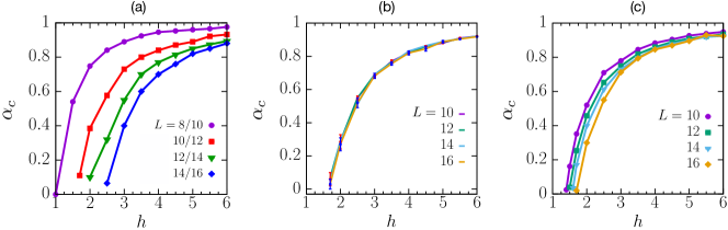
Figure 3: Phase diagram in $h-\alpha$ plane, where the critical correlation $\alpha_{c}(h)$ for the transition has been obtained for each value of $h$ from (a) the crossing point between $\langle r\rangle$ vs $\alpha$ curves of successive system sizes, (b) the location of the sign change in the power law exponent $b$ in $P_{1}(\lambda_{1})$ for different system sizes, and (c) the location where $P_{2}[\lambda_{2}=\ln(2)]$ vanishes for different system sizes. We notice strong system size dependence in (a), while the weakest system size dependence in using the criterion (b). In (b), the errorbars are obtained from errors in estimation of the exponent $b$.

At finite $\alpha$, the $h_{i}$s are correlated random variables. To see how the distribution changes with $\alpha$, it is instructive to look at the eigenvectors and eigenvalues of the covariance matrix. The eigenvectors represent the linear combinations of $h_{i}$s which are uncorrelated Gaussian random variables with the variances given by the eigenvalues. For our choice, $(1,1,....1)$ is an eigenvector with eigenvalue $h^{2}[1+(L-1)\alpha]$ and the rest of the degenerate eigenvalues are equal to $h^{2}(1-\alpha)$ with the eigenvectors lying in a $L-1$ dimensional subspace orthogonal to $(1,1,...1)$. As $\alpha\rightarrow 1$, the probability distributions along these orthogonal directions shrink to a delta function , i.e. all the coupling vectors lie along the $(1,1,...1)$ direction. This is the extremely correlated limit, where the magnetic fields in each realization are exactly same on all lattice sites. The value of this common magnetic field varies from one realization to another.

A schematic representation of how the distribution of the vector of couplings change with $h$ and $\alpha$ is shown in Fig. 1 (a) in the $h-\alpha$ plane (for $L=3$). Increasing $h$ at fixed $\alpha$ broadens the distribution of the length of these vectors while keeping their angular distribution same. Similarly increasing $\alpha$ while keeping $h$ fixed causes the angular distribution to narrow around the $(1,1,1)$ direction. In Fig. 1 (b) we plot the unit vectors corresponding to different sample realizations of the coupling vector on a unit sphere for $\alpha=0,~{}0.8,1.0$. The change of the angular distribution from an uniform distribution at $\alpha=0$ to a narrow distribution as $\alpha\rightarrow 1$ is clearly seen here. In Fig 1 (c), we plot the distribution of individual $h_{i}$s obtained from a single sample for a system of size $L=2000$ for the same values of $\alpha$ as in Fig. 1 (b). We plot two different distributions corresponding to two different samples. When the disorder is uncorrelated ($\alpha=0$), the distributions overlap, showing that the samples are statistically similar to each other. As $\alpha$ is increased, the overlap decreases, showing that couplings in a sample are more narrowly distributed than couplings taken from different samples. In the extreme limit of $\alpha=1$, we find that all couplings in a sample are same, but their value varies from one sample to another.

Our correlated disorder model has the simplicity that it can be tuned from uncorrelated to extremely correlated limit using a single parameter. Other models, where the covariance $C_{ij}$ depends on the separation between $i$ and $j$, introduce additional lengthscales in the problem, and tuning them from uncorrelated to extremely correlated limits require going to large system sizes, which are numerically not accessible.

MBL-ergodic transition with varying $\alpha$: We will first consider the fate of this system as $\alpha$ is tuned from $0$ to $1$ at a fixed value of $h$. We will focus our attention on the system at $h=4$, where the uncorrelated system ($\alpha=0$) is in a many-body localized phase. As we increase $\alpha$, the system undergoes a phase transition from the MBL to ergodic phase. We numerically diagonalize the Hamiltonian for a large number of disorder realizations and use the eigenvalues $E_{n}$ and eigenstate wavefunctions $\phi_{n}(i)$ in the middle third of the spectrum to construct several statistics to look at this transition:

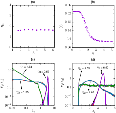
Figure 4: (a) The MBL-ergodic phase boundary in the $h-\alpha$ plane can be understood using a single parameter, the average sample variance $\eta^{2}$. The value of $\eta$ at the transition point, $\eta_{c}$, is plotted as a function of $h$. The constant $\eta_{c}(h)$ indicates that the MBL-ergodic transition is controlled by $\eta$. (b) $\langle r\rangle$ is plotted as a function of $\eta$ for several values of $(h,\alpha)$. The data collapses to a single curve (which changes from Wigner-Dyson to Poissonian value) with a small spread. (c)-(d): Distribution of (c) lowest entanglement eigenvalue $P_{1}(\lambda_{1})$ and (d) second lowest entanglement eigenvalue $P_{2}(\lambda_{2})$ are plotted for three values of $\eta$: $\eta_{1}=4.53$ (MBL phase), $\eta_{2}=1.85$ (transition point) and $\eta_{3}=0.52$ (ergodic phase). The curve for each value of $\eta$ is composed of data from three sets of $(h,\alpha)$ values. All curves with the same $\eta$ collapse to a single curve.

(i) The gap ratio $\langle r\rangle$: The level repulsion between the eigenstates can be parametrized by the ratio of the gap between successive energy eigenvalues, $r_{n}=(E_{n+1}-E_{n})/(E_{n}-E_{n-1})$. The gapmoment $\langle r\rangle$ is the average of this quantity, both over eigenstates in a disorder realization and over disorder realizations. $\langle r\rangle$ is expected to have an average value of $0.53$ in the ergodic phase corresponding to Wigner-Dyson distribution for level statistics, and an average value of $0.39$ in the MBL phase corresponding to a Poisson distribution for level statistics. In Fig. 2(a), we plot $\langle r\rangle$ as a function of $(1-\alpha)$ for different system sizes from $L=8$ to $L=16$ and see that the system clearly shows a transition from MBL to ergodic phase as $\alpha$ is increased. The location of the transition point, as measured from crossing of curves for increasing system sizes, vary over a broad range, similar to the transition for uncorrelated disorder as a function of $h$ oganesyan ; apal ; abhisek_kedar .

(ii) Kullback-Leibler divergences: The projection of an eigenstate $|\psi_{n}\rangle$ on a set of complete basis states (say the eigenstates of $\sigma^{z}_{i}$, $|\mu\rangle=\otimes_{i}|\sigma^{z}_{i}\rangle$), defines a probability distribution $p^{(n)}_{\mu}=|\langle\psi_{n}|\mu\rangle|^{2}$. One can construct the Kullback-Leibler divergences of the probability distributions obtained from successive energy eigenstates, $D_{KL}=\sum_{\mu}p^{(n)}_{\mu}\left(\ln{p^{(n)}_{\mu}\over{p^{(n-1)}_{\mu}}}\right)$ to compare how similar the successive eigenstates are. $D_{KL}$, averaged over adjacent pairs of eigenstates, and over disorder realizations, is expected to scale with system size in the MBL phase and should go to a value of $2$ in the ergodic phase  heisenberg . In Fig. 2(b) we have plotted $D_{KL}$ as a function of $(1-\alpha)$ for different system sizes. We notice that $D_{KL}$ reaches a constant value 2 when $\alpha\rightarrow 1$ (ergodic limit), and it scales with the system size as $\alpha$ decreases (MBL phase) heisenberg . Note that although $D_{KL}$ distinguishes the MBL phase from the ergodic phase, it is not a good indicator of the MBL-ergodic transition, since the crossover from $D_{KL}\sim L$ to $D_{KL}=2$ takes place over a wide range of $\alpha$ and is sensitive to the system size..

While the statistics described above show a gradual change from MBL to ergodic behaviour as a function of $\alpha$, sharper distinctions can be drawn from the distribution of entanglement spectra of reduced density matrices constructed from the energy eigenstates of the system nandkishore ; ent_spectrum ; abhisek_kedar . To see this, we consider a subsystem of size $L_{A}$ ($L_{A}=L/2$ for numerical data presented here). We start with the eigenstate $|\phi_{n}\rangle$, trace out the degrees of freedom lying outside the subsystem to construct the reduced density matrix $\hat{\rho}_{A}$. Here we look at the distribution of the lowest two entanglement eigenvalues of $\ln\hat{\rho}_{A}$, $\lambda_{1(2)}$:

(i) $P_{1}(\lambda_{1})$: The lowest entanglement eigenvalue $\lambda_{1}$ has a power law distribution in the range $0$ to $\ln(2)$, $P_{1}(\lambda_{1})\sim\lambda_{1}^{-b}$, with the exponent going from positive values in the MBL phase to negative values in the ergodic phase. The distribution shows characteristic kink at $\ln(2)$ in the MBL phase with an exponential decay at large values, while the ergodic phase shows a prominent peak at $\lambda_{1}\sim 3.5$. In Fig.. 2(c), we plot $P_{1}(\lambda_{1})$ for three values of $\alpha=0.4,0.8$, and 0.94 with a fixed $h=4$. We find that $\alpha=0.4$ is in the deep MBL phase, while $\alpha=0.94$ is in the ergodic phase. $\alpha=0.8$ shows the distribution at a point close to the transition.

(ii) $P_{2}(\lambda_{2})$: The second lowest entanglement eigenvalue $\lambda_{2}$ is always greater than $\ln(2)$. In the MBL phase the distribution is finite at $\lambda_{2}=\ln(2)$, while the ergodic phase shows exponentially small weight at this point. We note that a finite value of $P_{2}[\lambda_{2}=\ln(2)]$ corresponds to the exchange of exactly one bit information between the subsystem and its surroundings abhisek_kedar . In Fig. 2(d), we plot $P_{2}(\lambda_{2})$ for three values of $\alpha=0.4,0.8,$ and 0.94 with a fixed $h=4$. From the $P_{2}(\lambda_{2})$ curves, we once again find that $\alpha=0.4$ and $0.94$ corresponds respectively to systems deep in the MBL and ergodic phases, while the intermediate value $\alpha=0.8$ shows the distribution close to the transition point.

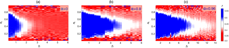
Figure 5: The density-plots of the average ratio of adjacent gaps $r$ are shown in energy-disorder ($\epsilon-h$) plane for three values of correlation (a) $\alpha=0$, (b) $\alpha=0.8$, and (c) $\alpha=0.96$. The energy $\epsilon$ is scaled by its range to lie between $0$ and $1$. With increase in $\alpha$, the blue region showing the ergodic states extend to larger values of $h$ and the transition from Wignar-Dyson to Poissonian statistics is broadened.

Additionally, we have also looked at the distribution of all entanglement eigenvalues which changes from a unimodal distribution in the ergodic phase to a bimodal distribution in the MBL phase and find the same MBL to ergodic transition as a function of $\alpha$ (see Appendix A for details).

The phase diagram: Having established that there is a MBL-ergodic transition as a function of $\alpha$ at large enough $h$, we now focus on the phase diagram of the system in the $h-\alpha$ plane, determined by fixing $h$ on a grid of values and tuning $\alpha$ in each case. We use three different criterion, with varying degree of system size dependence, to obtain the transition point $\alpha_{c}(h)$ : (i) The crossing point between the $\langle r\rangle$ vs $\alpha$ curves of successive system sizes. The phase diagram obtained from this criterion is plotted in Fig. 3(a) for different system sizes. (ii) The value of $\alpha$ where the exponent $b$ of the lowest entanglement eigenvalue distribution $P_{1}(\lambda_{1})$ changes sign. The phase diagram from this criterion is plotted in Fig. 3(b) for different system sizes. (iii) The value of $\alpha$ where $P_{2}[\lambda_{2}=\ln(2)]$ reaches $0$ (we use a threshold value of $10^{-3}$). The corresponding phase diagram is plotted in Fig. 3(c). All three criteria give qualitatively similar phase diagrams: at low $h<h_{c}(0)$, where $h_{c}(0)$ is the critical disorder for the uncorrelated system, the system is ergodic for all values of $\alpha$. For $h>h_{c}(0)$, there is a $\alpha_{c}(h)$ below which the system is in MBL phase, while it is in ergodic phase for $\alpha>\alpha_{c}(h)$. $\alpha_{c}(h)$ is a monotonically increasing function of $h$, rising rapidly from $0$ just above $h=h_{c}(0)$ and slowly saturating to $1$ as $h\rightarrow\infty$. In the next section we will derive an analytic expression for $\alpha_{c}(h)$. The phase boundaries obtained from the $\langle r\rangle$ vs $\alpha$ curves are strongly system size dependent, whereas the phase diagram obtained from change of slope of $b$ has the weakest size dependence. While the finite size systematics for the phase boundary obtained through (i) and (iii) sets the leading error estimates, we estimate the errors in phase boundary obtained by (ii) from errors in estimating $b$ (see Appendix B for the estimation of error in $b$).

The effective one-parameter model: If we consider the random magnetic fields at different sites in a particular disorder realization (or sample) as components of a vector, the parameter $\alpha$ controls the variation between these components. When $\alpha=1$, all the couplings in a particular sample are same; hence each realization is translation invariant, and the system should behave ergodically. The MBL vs ergodic behaviour of the system should thus be controlled by a measure of variation of the couplings within a sample. This can be captured by defining a sample/realization variance $\sigma^{2}=\frac{1}{L}\sum_{i}h_{i}^{2}-\left(\frac{1}{L}\sum_{i}h_{i}\right)^{2}$. $\sigma^{2}$ is a random variable, and its average over all disorder realizations is defined as $\eta^{2}=\langle\sigma^{2}\rangle$. For uncorrelated disorder ($\alpha=0$), one can easily show that for large system sizes, $\eta=h$ is just the standard deviation of the fields. On the other hand, for $\alpha=1$, $\sigma^{2}=0$ for every realization and hence $\eta=0$. For a generic $\alpha$, one can show that (see Appendix C for details)

$$\eta^{2}=h^{2}(1-\alpha)$$ (4)

We will now show that the phases and the phase diagram in the $h-\alpha$ plane can be understood in terms of this single parameter $\eta$. We first plot the value of $\eta$ at the phase transition points, $\eta_{c}(h)=h\sqrt{1-\alpha_{c}(h)}$, as a function of $h$ in Fig. 4(a). For $h>h_{c}(0)$, $\eta_{c}$ is constant, showing that the phase diagram can be understood in terms of this single parameter. Since $\eta_{c}=h_{c}(0)$ (for $\alpha=0$), one can use this to analytically obtain the phase boundaries in the $h-\alpha$ plane,

$$\alpha_{c}(h) =1-\left(\frac{h_{c}(0)}{h}\right)^{2} ~{}~{}\text{for}~{}~{}h\geq h_{c}(0)$$ (5)

$$=0 ~{}~{}\text{for}~{}~{}h<h_{c}(0)$$

Beyond the phase boundary, we now show that the behaviour of the system in the two phases across the transition is a function of a single parameter $\eta$. To see this, in Fig.  4(b), we plot the gapmoment $\langle r\rangle$ obtained at different $(h,\alpha)$ points as a function of $\eta$ and show that the data collapses to a single curve with a small spread. This data collapse is even more remarkable if one looks at the distribution of lowest entanglement eigenvalues. In Fig  4(c), we plot $P_{1}(\lambda_{1})$ for three different values of $\eta$, in the MBL, ergodic and the critical phase. Each curve is actually three curves (three different $(h,\alpha)$ values corresponding to the same value of $\eta$). These three curves are indistinguishable due to data collapse. Similar trends are seen in $P_{2}(\lambda_{2})$ plotted in Fig  4(d). This conclusively shows that there is a single parameter $\eta$ which is relevant for understanding the phases and the phase transitions in the $h-\alpha$ plane.

Mobility edge: Long-range correlations in disorder models are known to lead to mobility edges, even in non-interacting systems ganeshan ; modaksubroto1 . While the question of a many-body mobility edge has been debated sankar ; heisenberg ; modaksubroto2 ; monika ; mondaini , for spin chains with uncorrelated disorder, it has been shown heisenberg that at weak disorder, there is an energy range over which the gap statistics changes from its Wigner-Dyson distribution value of $0.51$ to its value in the Poisson limit ($0.39$). Due to finite size of the system, the change happens over a finite energy window. At large disorder, all states are many-body localized, leading to the disappearance of the mobility edge. In Fig. 5(a)-(c), we plot the gap statistics $r$ as a color plot in the energy-$h$ plane for three different values of correlation, $\alpha=0,0.8$ and $0.96$. In each case, we see a transition at weak disorder, with the ergodic states at the center of the spectrum extending to larger values of $h$ as $\alpha$ grows. This simply reflects the fact that the critical disorder increases with increasing $\alpha$. In addition, the transition energy range becomes larger as correlation $\alpha$ is increased, and a sharp “edge” is absent, as seen in Fig 5(a)-(c).

In summary, we have studied a spin chain with correlated disorder and have mapped out the phase diagram in the disorder-correlation plane. We show that the sample variance can be treated as a single parameter controlling the phases and phase transitions in the system. Using this, we can analytically find the phase boundary of the system. The usual picture of “mobility edges” separating localized and delocalized states at weak disorder in systems with uncorrelated disorder continues to hold in this case with some small modifications.

Appendix A Distribution of entanglement spectrum across the MBL-ergodic transition

In the main text we have studied the distribution of the lowest two entanglement eigenvalues, $P_{1}(\lambda_{1})$ and $P_{2}(\lambda_{2})$ to distinguish MBL and ergodic phases. We have also shown that the power law exponent of $P_{1}(\lambda_{1})$ below $\ln(2)$ and $P_{2}[\lambda_{2}=\ln(2)]$ can be used to track the transition accurately in the $\alpha-h$ plane. However one can also look at the whole entanglement spectrum $P(\lambda)$ to study the phase transition. In Fig. 6 we show $P(\lambda)$ for three values of $\alpha$, i.e. $\alpha=0.4,0.8$ and $0.94$. The system size is $L=16$ and the subsystem size is $L_{A}=8$. In the ergodic phase all eigenvalues of the reduced density matrix scale as $\rho_{n}\sim 1/2^{L_{A}}$, and hence we see a peak in the distribution for $\alpha=0.94$ around $\lambda\sim 8\ln(2)\approx 5.5$. As the system moves from the ergodic to MBL phase, a large weight appears at $\lambda=0$ which corresponds to the occurrence of product states abhisek_kedar . Therefore, MBL phase is characterized by the existence of two peaks, one near $\lambda=0$ and another corresponding peak at large $\lambda$. The MBL-ergodic transition can be tracked by tracking the appearance of the $\lambda=0$ peak nandkishore . Using this metric, we see that we can reproduce the MBL-ergodic transition as a function of $\alpha$ discussed in the main text.

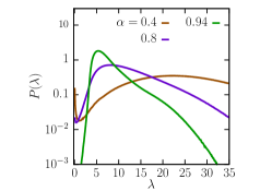
Figure 6: The distribution of the full entanglement spectrum $P(\lambda)$ for system size $L=16$ and subsystem size $L_{A}=8$ for different values of $\alpha$ for fixed $h=4$. The distribution shows a peak in the ergodic phase ($\alpha=0.94$) near $\lambda\sim 8\ln(2)$, while it is characterized by two peaks in the MBL phase ($\alpha=0.4$). At $\alpha=0.8$ the system is near the transition. The appearance of the peak near $\lambda=0$ can be used to track the transition.

Appendix B Estimation of error in the phase diagram obtained from the power-law exponent $b$

To draw the phase diagram in the $h-\alpha$ plane, we have used three different criteria in the main text. We have seen that the phase boundary obtained from the sign change of the power-law exponent $b$ of $P_{1}(\lambda_{1})$ has the weakest system size dependence. Therefore it is useful to estimate the error in drawing the phase boundary using this criterion. In Fig. 3(b) of the main text we have plotted the phase diagram and the corresponding error bars. Here we provide the technical details in the estimation of errors. For a given $h$, we move on a grid of $\alpha$ and fit $P_{1}(\lambda_{1})$ for each $\alpha$ in the range $0<\lambda_{1}<\ln(2)$ with a power law $P_{1}(\lambda_{1})\sim\lambda_{1}^{-b}$. This gives us a standard error of fitting in $b$, $\Delta b$. We estimate $\alpha_{c}(h)$ by tracking the sign change in $b$ as a function of $\alpha$. Similarly we estimate the error in $\alpha_{c}(h)$ by tracking the sign change in $b+\Delta b$ and $b-\Delta b$ as a function of $\alpha$. This is used to construct the errorbars shown in Fig. 2.

Appendix C Relation between $\eta,h$ and $\alpha$

In this Appendix we will calculate the relation between $\eta,h$ and $\alpha$ used in the main text. We consider a sample of $L$ random variables $h_{i}$ drawn from a correlated Gaussian distribution with standard deviation $h$ and correlation $\alpha$. We define $\bar{h}={1\over L}\sum_{i}h_{i}$ and $\sigma^{2}=\frac{1}{L}\sum_{i}h_{i}^{2}-\left(\frac{1}{L}\sum_{i}h_{i}\right)^{2}$ to be the mean value and the variance within the sample respectively. The average of sample variance over all disorder realization $\eta^{2}=\langle\sigma^{2}\rangle$ is given by,

$$\eta^{2} =\frac{1}{L}\Big{\langle}\sum_{i=1}^{L}(h_{i}-\bar{h})^{2}\Big{\rangle}$$

$$=(h^{2}-\langle{\bar{h}}^{2}\rangle)$$ (6)

In this case,

$$\bar{h}^{2} ={1\over L^{2}}\left[\sum_{i}^{n}h_{i}^{2}+h_{1}(h_{2}+h_{3}+...+h_{L})\right.$$ (7)

$$\!\!\!\!\!\!+h_{2}(h_{1}+h_{3}+...+h_{L})+...+h_{L}(h_{1}+h_{2}+...+h_{L-1})\Big{]},$$

Disorder average of $\bar{h}^{2}$ yields $\langle\bar{h}^{2}\rangle={1\over L^{2}}\left[Lh^{2}+L(L-1)\alpha h^{2}\right]$. Using this in Eqn. 6 we find $\eta^{2}=(1-\alpha)h^{2}+{\cal O}(1/L)$, which reduces to Eq. 4 in the main text for large $L$.

References

- [1] Igor V Gornyi, Alexander D Mirlin, and Dmitry G Polyakov. Interacting electrons in disordered wires: Anderson localization and low-t transport. Physical review letters, 95(20):206603, 2005.
- [2] Denis M Basko, Igor L Aleiner, and Boris L Altshuler. Metal–insulator transition in a weakly interacting many-electron system with localized single-particle states. Annals of physics, 321(5):1126–1205, 2006.
- [3] Rahul Nandkishore and David A Huse. Many-body localization and thermalization in quantum statistical mechanics. Annu. Rev. Condens. Matter Phys., 6(1):15–38, 2015.
- [4] Ehud Altman. Many-body localization and quantum thermalization. Nature Physics, 14(10):979–983, 2018.
- [5] Fabien Alet and Nicolas Laflorencie. Many-body localization: An introduction and selected topics. Comptes Rendus Physique, 19(6):498–525, 2018.
- [6] Michael Schreiber, Sean S Hodgman, Pranjal Bordia, Henrik P Lüschen, Mark H Fischer, Ronen Vosk, Ehud Altman, Ulrich Schneider, and Immanuel Bloch. Observation of many-body localization of interacting fermions in a quasirandom optical lattice. Science, 349(6250):842–845, 2015.
- [7] Jacob Smith, Aaron Lee, Philip Richerme, Brian Neyenhuis, Paul W Hess, Philipp Hauke, Markus Heyl, David A Huse, and Christopher Monroe. Many-body localization in a quantum simulator with programmable random disorder. Nature Physics, 12(10):907–911, 2016.
- [8] Josh M Deutsch. Quantum statistical mechanics in a closed system. Physical review a, 43(4):2046, 1991.
- [9] Mark Srednicki. Chaos and quantum thermalization. Physical review e, 50(2):888, 1994.
- [10] Zhi-Cheng Yang, Claudio Chamon, Alioscia Hamma, and Eduardo R Mucciolo. Two-component structure in the entanglement spectrum of highly excited states. Physical review letters, 115(26):267206, 2015.
- [11] Scott D Geraedts, Nicolas Regnault, and Rahul M Nandkishore. Characterizing the many-body localization transition using the entanglement spectrum. New Journal of Physics, 19(11):113021, 2017.
- [12] Abhisek Samanta, Kedar Damle, and Rajdeep Sensarma. Tracking the many-body localized to ergodic transition via extremal statistics of entanglement eigenvalues. Physical Review B, 102(10):104201, 2020.
- [13] Vadim Oganesyan and David A Huse. Localization of interacting fermions at high temperature. Physical review b, 75(15):155111, 2007.
- [14] Arijeet Pal and David A Huse. Many-body localization phase transition. Physical review b, 82(17):174411, 2010.
- [15] David J Luitz, Nicolas Laflorencie, and Fabien Alet. Many-body localization edge in the random-field heisenberg chain. Physical Review B, 91(8):081103, 2015.
- [16] Marko Žnidarič, Tomaž Prosen, and Peter Prelovšek. Many-body localization in the heisenberg x x z magnet in a random field. Physical Review B, 77(6):064426, 2008.
- [17] Jonas A Kjäll, Jens H Bardarson, and Frank Pollmann. Many-body localization in a disordered quantum ising chain. Physical review letters, 113(10):107204, 2014.
- [18] Maxime Dupont and Nicolas Laflorencie. Many-body localization as a large family of localized ground states. Physical Review B, 99(2):020202, 2019.
- [19] Hugo Théveniaut, Zhihao Lan, and Fabien Alet. Many-body localization transition in a two-dimensional disordered quantum dimer model. arXiv preprint arXiv:1902.04091, 2019.
- [20] Shankar Iyer, Vadim Oganesyan, Gil Refael, and David A Huse. Many-body localization in a quasiperiodic system. Physical Review B, 87(13):134202, 2013.
- [21] FM Izrailev and AA Krokhin. Localization and the mobility edge in one-dimensional potentials with correlated disorder. Physical review letters, 82(20):4062, 1999.
- [22] Alexander Croy, Philipp Cain, and Michael Schreiber. Anderson localization in 1d systems with correlated disorder. The European Physical Journal B, 82(2):107–112, 2011.
- [23] Soumi Ghosh, Atithi Acharya, Subhayan Sahu, and Subroto Mukerjee. Many-body localization due to correlated disorder in fock space. Physical Review B, 99(16):165131, 2019.
- [24] Sthitadhi Roy and David E Logan. Fock-space correlations and the origins of many-body localization. Physical Review B, 101(13):134202, 2020.
- [25] Sthitadhi Roy, JT Chalker, and David E Logan. Percolation in fock space as a proxy for many-body localization. Physical Review B, 99(10):104206, 2019.
- [26] Sthitadhi Roy and David E Logan. Localization on certain graphs with strongly correlated disorder. Physical Review Letters, 125(25):250402, 2020.
- [27] Scott D Geraedts, Rahul Nandkishore, and Nicolas Regnault. Many-body localization and thermalization: Insights from the entanglement spectrum. Physical Review B, 93(17):174202, 2016.
- [28] Sriram Ganeshan, JH Pixley, and S Das Sarma. Nearest neighbor tight binding models with an exact mobility edge in one dimension. Physical review letters, 114(14):146601, 2015.
- [29] Ranjan Modak, Soumi Ghosh, and Subroto Mukerjee. Criterion for the occurrence of many-body localization in the presence of a single-particle mobility edge. Physical Review B, 97(10):104204, 2018.
- [30] Xiaopeng Li, Sriram Ganeshan, JH Pixley, and S Das Sarma. Many-body localization and quantum nonergodicity in a model with a single-particle mobility edge. Physical review letters, 115(18):186601, 2015.
- [31] Ranjan Modak and Subroto Mukerjee. Many-body localization in the presence of a single-particle mobility edge. Physical review letters, 115(23):230401, 2015.
- [32] Thomas Kohlert, Sebastian Scherg, Xiao Li, Henrik P Lüschen, Sankar Das Sarma, Immanuel Bloch, and Monika Aidelsburger. Observation of many-body localization in a one-dimensional system with a single-particle mobility edge. Physical review letters, 122(17):170403, 2019.
- [33] Xingbo Wei, Chen Cheng, Gao Xianlong, and Rubem Mondaini. Investigating many-body mobility edges in isolated quantum systems. Physical Review B, 99(16):165137, 2019.