Reentrant Correlated Insulators in Twisted Bilayer Graphene at 25T ($2\pi$ Flux)

Abstract

Twisted bilayer graphene (TBG) is remarkable for its topological flat bands, which drive strongly-interacting physics at integer fillings, and its simple theoretical description facilitated by the Bistritzer-MacDonald Hamiltonian, a continuum model coupling two Dirac fermions. Due to the large moiré unit cell, TBG offers the unprecedented opportunity to observe reentrant Hofstadter phases in laboratory-strength magnetic fields near 25T. This Letter is devoted to magic angle TBG at $2\pi$ flux where the magnetic translation group commutes. We use a newly developed gauge-invariant formalism to determine the exact single-particle band structure and topology. We find that the characteristic TBG flat bands reemerge at $2\pi$ flux, but, due to the magnetic field breaking $C_{2z}\mathcal{T}$, they split and acquire Chern number $\pm 1$. We show that reentrant correlated insulating states appear at $2\pi$ flux driven by the Coulomb interaction at integer fillings, and we predict the characteristic Landau fans from their excitation spectrum. We conjecture that superconductivity can also be re-entrant at $2\pi$ flux.

Introduction. Twisted bilayer graphene (TBG) is the prototypical moiré material obtained from rotating two graphene layers by an angle $\theta$. Near the magic angle $\theta=1.05^{\circ}$, the two bands near charge neutrality flatten to a few meV, pushing the system into the strong-coupling regime and unravelling a rich landscape of correlated insulators and superconductors Cao et al. (2018, 2018); Kim et al. (2017); Kennes et al. (2021); Balents et al. (2020); Liu and Dai (2021); Chu et al. (2020). Due to the large moiré unit cell, magnetic fluxes of $2\pi$ are achieved at only 25T. In Hofstadter tight-binding models, such as the square lattice with Peierls substitution, the $2\pi$-flux and zero-flux models are equivalent, although the situation is more complicated in TBG Herzog-Arbeitman et al. (2020). This begs the question: do insulating and superconducting phases of TBG repeat at 25T?

We study the Bistritzer-MacDonald (BM) Hamiltonian Bistritzer and MacDonald (2011), describing the interlayer moiré-scale coupling of the graphene Dirac fermions within a single valley, which has established itself as a faithful model of the emergent TBG physics. We write the BM Hamiltonian in the particle-hole symmetric approximation as

$$H_{BM}(\mathbf{r})=\begin{pmatrix}-i\hbar v_{F}\boldsymbol{\nabla}\cdot\boldsymbol{\sigma}&h.c.\\ \sum_{j=1}^{3}T_{j}e^{2\pi i\mathbf{q}_{j}\cdot\mathbf{r}}&-i\hbar v_{F}\boldsymbol{\nabla}\cdot\boldsymbol{\sigma}\\ \end{pmatrix}\ .$$ (1)

Here $\mathbf{q}_{j}=C_{3z}^{j-1}\mathbf{q}_{1}$ are the inter-layer momentum hoppings, $\mathbf{q}_{1}=(0,4\sin(\frac{\theta}{2})/3a_{g})$, and $a_{g}=.246$nm is the graphene lattice constant. The BM couplings $T_{1}=w_{0}\sigma_{0}+w_{1}\sigma_{1}$, $T_{j+1}=\exp(\frac{2\pi i}{3}j\sigma_{3})T_{1}\exp(-\frac{2\pi i}{3}j\sigma_{3})$ act on the sublattice indices of the Dirac fermions, and $\sigma_{j}$ are the Pauli matrices. The lattice potential scale is $w_{1}=110$meV with $w_{0}/w_{1}=.6$ - $.8$ Koshino et al. (2018); Das et al. (2021) and the kinetic energy scale is $2\pi\hbar v_{F}|\mathbf{q}_{1}|=190$meV. The spectrum of $H_{BM}(\mathbf{r})$ has been thoroughly investigated Song et al. (2019); Tarnopolsky et al. (2019); Bernevig et al. (2021a); Song et al. (2021); Wang et al. (2020); Chen et al. (2020).

The salient feature of the BM model from the Hofstadter perspective is the size of the moiré unit cell. After a unitary transform by $\text{diag}(e^{i\pi\mathbf{q}_{1}\cdot\mathbf{r}},e^{-i\pi\mathbf{q}_{1}\cdot\mathbf{r}})$, $H_{BM}(\mathbf{r})$ is put into Bloch form and is periodic under translations by $\mathbf{a}_{i}$, the moiré lattice vectors Zou et al. (2018). Near the magic angle, the moiré unit cell area $\Omega=|\mathbf{a}_{1}\times\mathbf{a}_{2}|$ is a factor of $\theta^{-2}\sim 3000$ times larger than the graphene unit cell. This dramatic increase in size brings the Hofstadter regime

$$\phi=eB\Omega/\hbar\sim 2\pi$$ (2)

within reach, showcasing physics which is only possible in strong flux Hofstadter (1976); Herzog-Arbeitman et al. (2020); Wang and Santos (2020); Albrecht et al. (2001); Bernevig and Hughes (2013); Lu et al. (2020); Dean et al. (2013). Here $e/2\pi\hbar$ is the flux quantum (henceforth $e\!=\!\hbar\!=1\!$) and the magnetic field $B$ is near $25$T at $\phi=2\pi$ and $\theta=1.05^{\circ}$. In the lattice Hofstadter problem, there is an exact periodicity in flux depending on the orbitals Herzog-Arbeitman et al. (2020). This is no longer true in the continuum model Eq. (1). Nevertheless we find that the flat bands and correlated insulators are revived at $\phi=2\pi$.

A constant magnetic field $\epsilon_{ij}\partial_{i}A_{j}=B>0$ (repeated indices are summed) is incorporated into Eq. (1) via the canonical substitution $-i\boldsymbol{\nabla}\to\boldsymbol{\pi}=-i\boldsymbol{\nabla}-\mathbf{A}(\mathbf{r})$ yielding $H^{\phi}_{BM}$. Because the vector potential breaks translation symmetry, the spectrum in flux cannot be solved using Bloch’s theorem. This problem has a long history with many approaches Zak (1964a, b); Brown (1969); Streda (1982); Wannier (1978); Pereira et al. (2007); Xiao et al. (2010); Gumbs et al. (1995); Bistritzer and MacDonald (2011); Hejazi et al. (2019); Crosse et al. (2020); Lian et al. (2021a). However, we found that none accommodated the more demanding topological calculations essential for understanding TBG. Our separate work Ref. Herzog-Arbeitman et al. contains technical calculations and proofs of formulae for the band structure, non-abelian Wilson loop, and many-body form factors. We apply the theory here to study the single-particle and many-body physics of TBG at $2\pi$ flux. Accompanying this paper, Ref. Das et al. experimentally confirms our prediction of re-entrant correlated insulators in TBG at $2\pi$ flux.

Magnetic Bloch Theorem.

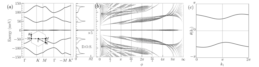
Figure 1: TBG in flux. (a) The band structure and density of states at $\phi=2\pi$, $w_{0}/w_{1}=0.8$, and $\theta=1.05^{\circ}$ reveal $\sim 1.5$meV flat bands with a $40$meV gap. (b) The full Hofstadter spectrum shows the flat bands remain gapped at all flux. (c) Calculating the Wilson loop $W(k_{1})$ of the two flat bands shows that, due to $C_{2}\mathcal{T}$ breaking, the topology of the flat bands is trivial when they are connected.

In zero flux, the translation group of a crystal allows one to construct an orthonormal basis of momentum eigenstates labeled by $\mathbf{k}$ in the Brillouin zone (BZ) and the spectrum is given by the Bloch Hamiltonian at each $\mathbf{k}$. A similar construction can be followed at $2\pi$ flux where the magnetic translation group commutes. To begin, define the canonical momentum $\pi_{\mu}=-i\partial_{\mu}-A_{\mu}$ and guiding centers $Q_{\mu}=\pi_{\mu}-B\epsilon_{\mu\nu}x_{\nu}$ which obey the (gauge-invariant) algebra

$$\hbox{}[\pi_{\mu},\pi_{\nu}]=iB\epsilon_{\mu\nu},\ [Q_{\mu},Q_{\nu}]=-iB\epsilon_{\mu\nu},\ [\pi_{\mu},Q_{\nu}]=0,$$ (3)

forming two decoupled algebras which are isomorphic to the free oscillator algebra. The kinetic term of Eq. (1) contains only $\pi_{\mu}$ operators and commutes with the guiding centers $Q_{\mu}$. The Landau level ladder operators

$$a =(\pi_{x}+i\pi_{y})/\sqrt{2B},\quad a^{\dagger}=(\pi_{x}-i\pi_{y})/\sqrt{2B}$$ (4)

obeying $[a,a^{\dagger}]=1$ allow the Dirac Hamiltonian to be exactly solved in flux Xiao et al. (2010). Without a potential term, the $Q_{\mu}$ operators generate the macroscopic Landau level degeneracy. A potential term $U(\mathbf{r})$ will break the degeneracy. If $U(\mathbf{r})$ is periodic, the magnetic translation operators $T_{\mathbf{a}_{i}}=e^{i\mathbf{a}_{i}\cdot\mathbf{Q}}$ commute with $H_{BM}^{\phi}$ because

$$T_{\mathbf{a}_{i}}U(\mathbf{r})T^{\dagger}_{\mathbf{a}_{i}}=U(\mathbf{r}+\mathbf{a}_{i})=U(\mathbf{r}),\text{ and }\ [T_{\mathbf{a}_{i}},\pi_{\mu}]=0$$ (5)

using Eq. (3) and the Baker-Campbell-Hausdorff (BCH) formula. The magnetic translation operators obey the projective representation $T_{\mathbf{a}_{1}}T_{\mathbf{a}_{2}}=e^{i\phi}T_{\mathbf{a}_{2}}T_{\mathbf{a}_{1}}$ Zak (1964a). For generic flux, $T_{\mathbf{a}_{1}}$ and $T_{\mathbf{a}_{2}}$ do not commute, creating a characteristic fractal spectrum Hofstadter (1976). Our interest in this work is the Hofstadter regime where $\phi=2\pi$, the magnetic translation operators commute, and the spectrum consists of bands labeled by a “momentum” $\mathbf{k}=k_{1}\mathbf{b}_{1}+k_{2}\mathbf{b}_{2}$, $k_{i}\in(-\pi,\pi)$ and $\mathbf{a}_{i}\cdot\mathbf{b}_{j}=\delta_{ij}$. To determine the band structure, one needs a basis of magnetic translation group irreps on infinite boundary conditions. Our results rest on the following construction at $\phi=2\pi$:

$$\ket{\mathbf{k},n,\alpha,l}=\frac{1}{\sqrt{\mathcal{N}(\mathbf{k})}}\sum_{\mathbf{R}}e^{-i\mathbf{k}\cdot\mathbf{R}}T_{\mathbf{a}_{1}}^{\mathbf{R}\cdot\mathbf{b}_{1}}T_{\mathbf{a}_{2}}^{\mathbf{R}\cdot\mathbf{b}_{2}}\ket{n,\alpha,l}$$ (6)

where $\mathbf{R}$ is the moiré Bravais lattice, $\alpha=A,B$ is the sublattice index, $l=\pm 1$ is the layer index, and $n$ is the Landau level defined by $\ket{n,\alpha,l}=\frac{a^{{\dagger}\,n}}{\sqrt{n!}}\ket{0,\alpha,l},\ a\ket{0,\alpha,l}=0$. A similar construction was used in Ref. Herzog-Arbeitman et al. (2020) to identify a projective representation of the magnetic space group $1^{\prime}$ in the Hofstadter Hamiltonian of a tight-binding model. The states in Eq. (15) are magnetic translation group eigenstates obeying $T_{\mathbf{a}_{i}}\ket{\mathbf{k},n,\alpha,l}=e^{i\mathbf{k}\cdot\mathbf{a}_{i}}\ket{\mathbf{k},n,\alpha,l}$, which immediately proves their orthogonality at different $\mathbf{k}$. Orthogonality at different $n$ follows because $\ket{\mathbf{k},n}$ are eigenstates of the Hermitian operator $a^{\dagger}a$ with eigenvalue $n$. The normalization $\mathcal{N}(\mathbf{k})$ is determined by requiring orthonormality $\braket{\mathbf{k}^{\prime},m}{\mathbf{k},n}=(2\pi)^{2}\delta_{mn}\delta(\mathbf{k}-\mathbf{k}^{\prime})$ and can be expressed in terms of theta functions (App. A). We find that $\mathcal{N}(\mathbf{k}^{*})=0$, indicating that the states are not well-defined at $\mathbf{k}^{*}=\pi\mathbf{b}_{1}+\pi\mathbf{b}_{2}$. This is because the states in Eq. (15) are built from Landau levels $\ket{n,\alpha,l}$ which carry a Chern number, but Chern states cannot be periodic and well-defined everywhere in the BZ Brouder et al. (2007). On infinite boundary conditions, the point $\mathbf{k}^{*}$ is a set of measure zero in the BZ, and we prove in Ref. Herzog-Arbeitman et al. that the basis in Eq. (15) is complete with the exception of pathological examples that do not occur when the wavefunctions are suitably smooth.

The basis states in Eq. (15) yield a simple expression for the magnetic Bloch Hamiltonian

$$\hbox{}(2\pi)^{2}\delta(0)[H_{BM}^{\phi=2\pi}(\mathbf{k})]_{mn,\alpha\beta,ll^{\prime}}=\braket{\mathbf{k},m,\alpha,l}{H^{\phi=2\pi}_{BM}}{\mathbf{k},n,\beta,l^{\prime}}\ .$$ (7)

The matrix elements of Eq. (7) can be computed exactly to obtain an expression for $H_{BM}^{\phi=2\pi}(\mathbf{k})$ (App. A). Truncating to $N_{LL}$ Landau levels, we obtain a finite $4N_{LL}\times 4N_{LL}$ matrix that can be diagonalized at each $\mathbf{k}$ to produce a band structure. This is similar to the zero flux expansion of $H_{BM}$ on a plane wave basis, where high momentum modes are truncated. As computed in Fig. 1a, the famous flat bands of magic-angle TBG remain at $2\pi$ flux suggesting that the system will be dominated by strong interactions. We use the open momentum space technique Lian et al. (2021a) to obtain the Hofstadter spectrum (Fig. 1b) which shows the evolution of the higher energy passive bands. At $2\pi$ flux, full density Bloch-like flat bands reappear at charge neutrality and are the focus of this work.

Topology of the Flat bands. Similar to the zero flux TBG flat bands, the reentrant flat bands at $2\pi$ flux have a very small bandwidth of $\sim 1$ meV. However, their topology is quite different due to the breaking of crystalline symmetries by magnetic field. Let us review the zero flux model. Ref. Song et al. (2019) showed that the space group $p6^{\prime}2^{\prime}2$ of the BM Hamiltonian (Eq. (1)) was generated by $C_{3z},C_{2x},$ and $C_{2z}\mathcal{T}$ and also featured an approximate unitary particle-hole operator $P$. Notably, $C_{2z}\mathcal{T}$ alone is sufficient to protect the gapless Dirac points and fragile topology of the flat bands Song et al. (2019).

Because a perpendicular magnetic field is reversed by time-reversal and $C_{2x}$ symmetries (while it is invariant under in-plane rotations), the $C_{2x}$ and $C_{2z}\mathcal{T}$ symmetries are broken in flux Herzog-Arbeitman et al. (2020). Thus, the space group of $H_{BM}^{\phi}$ is reduced to $p31m^{\prime}$ which is generated by $C_{3z}$ and $M\mathcal{T}\equiv C_{2x}C_{2z}\mathcal{T}$. $P$ also remains a symmetry. Without $C_{2z}\mathcal{T}$, the system changes substantially. The most direct way to assess the topology at $2\pi$ flux is to calculate the non-Abelian Wilson loop. To do so, we need an expression for the Berry connection $\mathcal{A}^{MN}(\mathbf{k})$ where $M,N$ index the occupied bands. At $2\pi$ flux, the Berry connection ${\cal A}_{i}={\mathbf{b}}_{i}\cdot{\cal A}$ contains new contributions Herzog-Arbeitman et al. :

$$\mathcal{A}_{i}^{MN}(\mathbf{k}) =[U^{\dagger}(\mathbf{k})(i\partial_{k_{i}}-\epsilon_{ij}\tilde{Z}_{j})U(\mathbf{k})]^{MN}$$ (8)

$$\qquad\qquad-\delta^{MN}\epsilon_{ij}\partial_{k_{j}}\log\sqrt{\mathcal{N}(\mathbf{k})}$$

where $U(\mathbf{k})$ is the matrix of eigenvectors and $M,N$ span the occupied bands. In the case of the TBG flat bands, $U(\mathbf{k})$ is a $4N_{LL}\times 2$ matrix. The Abelian term in the second line of Eq. (8) is an exact expression for the Berry connection of a Landau level which is discussed at length in Ref. Herzog-Arbeitman et al. and accounts for the Chern number of the basis states. The non-Abelian term $\tilde{Z}_{j}$ acts nontrivially on the Landau level indices (App. A). We numerically calculate the Wilson loop Alexandradinata et al. (2014) over the flat bands in Fig. 1(c) which shows no winding. Hence the fragile topology of the flat bands, which was protected by $C_{2z}\mathcal{T}$, is broken in flux. However, we calculate that the neighboring passive bands are gapped (unlike at zero flux) and carry nonzero Chern numbers (App. B). They are dispersive Landau levels originating from the Rashba point of the passive bands at zero flux Das et al. (2021).

To gain a deeper understanding of the topology at $2\pi$ flux, we study the band representation $\mathcal{B}$ with topological quantum chemistry Bradlyn et al. (2017); Aroyo et al. (2006a, b). First, Fig. 1b demonstrates that the flat bands remain gapped from all other bands in flux. This is despite the fragile topology of TBG, verifying the prediction of Ref. Herzog-Arbeitman et al. (2020). $C_{2z}$ symmetry, however is sufficient to protect a gap closing in concert with the fragile topology. Thus $\mathcal{B}$ can be simply obtained by reducing the band representation of TBG in zero flux derived in Ref. Song et al. (2019) to $p31m^{\prime}$. We find

$$\mathcal{B}=2\Gamma_{1}+K_{2}+K_{3}+K_{2}^{\prime}+K_{3}^{\prime}=A_{2b}\uparrow p31m^{\prime}$$ (9)

which is an elementary band representation and is not topological. The irreps are defined

$$\begin{array}[]{r|rr}3m^{\prime}&1&C_{3z}\\ \hline\cr\Gamma_{1}&1&1\\ \end{array},\quad\begin{array}[]{r|rr}3&1&C_{3z}\\ \hline\cr K_{2}&1&e^{\frac{2\pi i}{3}}\\ K_{3}&1&e^{-\frac{2\pi i}{3}}\\ \end{array},\quad\begin{array}[]{r|rr}3&1&C_{3z}\\ \hline\cr K^{\prime}_{3}&1&e^{\frac{2\pi i}{3}}\\ K^{\prime}_{2}&1&e^{-\frac{2\pi i}{3}}\\ \end{array}$$ (10)

and $A_{2b}$ denotes two one-dimensional irreps of $s$ orbitals placed at the corners of the moiré unit cell, which matches the charge distribution at zero flux Song et al. (2019); Kang and Vafek (2018); Koshino et al. (2018). Another simple observation is that the total Chern number of the two flat bands is zero, so the flat bands cannot be modeled by decoupled Landau levels despite the strong flux, which demonstrates the importance of our exact approach. Consulting the Bilbao Crystallographic Server, we observe that Eq. (9) is decomposable in momentum space Cano et al. (2018a, b); Bradlyn et al. (2019), meaning that $\mathcal{B}$ may be split into two disconnected bands:

$$\mathcal{B}=\mathcal{B}_{+}+\mathcal{B}_{-}=(\Gamma_{1}\!+\!K_{2}\!+\!K_{3}^{\prime})+(\Gamma_{1}\!+\!K_{3}\!+\!K_{2}^{\prime})$$ (11)

where $\mathcal{B}_{\pm}$ carries Chern number $C=\pm 1$ mod $3$ Fang et al. (2012). The irreps of $\mathcal{B}_{\pm}$ at the $K$ and $K^{\prime}$ points are related by the anti-unitary operator $M\mathcal{T}$ which obeys $C_{3z}M\mathcal{T}=M\mathcal{T}C_{3z}^{\dagger}$, so Eq. (11) is the only allowed decomposition. We show below that the addition of $P$, which is not part of the irrep classification (it is not a crystallographic symmetry), forbids this splitting.

Eq. (11) suggests a remarkable similarity to the topology of the flat bands at zero flux, where $C_{2z}\mathcal{T}$ enforces connected bands whose Wilson loop eigenvalues wind in opposite directions Liu et al. (2019); Song et al. (2019, 2021); Ahn et al. (2019). $C_{2z}\mathcal{T}$ is crucial to protecting the fragile topology, which would otherwise be trivialized from the cancelation of the winding. At $2\pi$ flux, breaking $C_{2z}\mathcal{T}$ destroys the fragile topology but allows the bands to split and carry opposite non-zero Chern numbers. Thus in flux, the fragile topology in the two TBG flat bands is replaced by stable topology as the bands split and acquire a Chern number. These bands carry opposite Chern number, but they cannot annihilate with each other: $M\mathcal{T}$ symmetry ensures any band touching come in pairs so the Chern numbers can only change in multiples of two. To understand the mechanism which splits the flat bands, we re-examine $P$ which has so far been neglected. $P$ is not an exact (but still a very good) symmetry of TBG and only anti-commutes when terms of $O(\theta)$ are dropped Song et al. (2019, 2021). We incorporate the exact $\theta$ dependence into the kinetic terms of Eq. (1), breaking $P$ and opening a $\sim.5$meV gap between the flat bands at $K$ and $K^{\prime}$ and verify the Chern number decomposition in Eq. (11) from the Wilson loop (App. C).

The particle-hole approximation prevents the Chern decomposition because $P$ and $C_{3z}$ enforce gapless points at $K$ and $K^{\prime}$ as we now show. Observe that the $K$ and $K^{\prime}$ points are symmetric under the anti-commuting symmetry $\mathcal{P}=PM\mathcal{T}$ because $P$ takes $\mathbf{k}\to-\mathbf{k}$ and $M\mathcal{T}$ takes $(k_{x},k_{y})\to(k_{x},-k_{y})$ Song et al. (2019). $\mathcal{P}$ is anti-unitary and obeys $C_{3z}\mathcal{P}=\mathcal{P}C_{3z}^{\dagger}$. As such, a state $\ket{\omega}$ of energy $E\neq 0$ and $C_{3z}$ eigenvalue $\omega$ ensures a distinct state $\mathcal{P}\ket{\omega}$ with $C_{3z}$ eigenvalue $\omega$ and energy $-E$. Thus all states at $E\neq 0$ come in $\mathcal{P}$-related pairs with the same $C_{3z}$ eigenvalue. We see that the irreps of $\mathcal{B}$ at $K$ and $K^{\prime}$ cannot be gapped (they are pinned to $E=0$) without violating $\mathcal{P}$ because they have different $C_{3z}$ eigenvalues.

Coulomb Groundstates. We have derived the spectrum and topology of TBG at $2\pi$ flux, thoroughly studying its single-particle physics. When considering many-body states, we must include the spin and valley degrees of freedom. The low energy states in TBG come from the two graphene valleys which we index by $\eta=\pm 1$. The valleys are interchanged by $C_{2z}$ which is unbroken by flux, and hence the flat bands are each four-fold degenerate. To split the degeneracy, we consider adding the interaction

$$H_{int}=\frac{1}{2\Omega_{tot}}\sum_{\mathbf{q}}V(\mathbf{q})\bar{\rho}_{-\mathbf{q}}\bar{\rho}_{\mathbf{q}},\quad\bar{\rho}_{\mathbf{q}}=\int d^{2}r\,e^{-i\mathbf{q}\cdot\mathbf{r}}\bar{n}(\mathbf{r})$$ (12)

where $V(\mathbf{q})>0$ is the screened Coulomb potential Bernevig et al. (2021b); Liu et al. (2021), $\bar{n}(\mathbf{r})$ is the total electron density (summed over valley and spin) measured from charge neutrality, and $\Omega_{tot}$ is the area of the sample. We now discuss the symmetries of the many-body Hamiltonian. In zero flux, the single-particle and interaction terms conserve spin, charge, and valley, so there is an exact $U(2)\times U(2)$ symmetry group. It is also natural to work in a strong coupling expansion where we project $H_{int}$ onto the two flat bands and neglect their kinetic energy entirely. This is a very reliable approximation because the bandwidth is $O(1)$ meV and the interaction strength is $\sim 20$meV. In this limit, $C_{2z}P$ commutes with the projected $H_{int}$ operator and the symmetry group is promoted to $U(4)$Bernevig et al. (2021b); Vafek and Kang (2020).

We now discuss the fate of the $U(4)$ symmetry in flux. At $B\sim 25$T, the Zeeman effect shifts the energy of the spin $\pm 1/2$ electrons by $\pm\mu_{B}B=\pm 1.4$meV where $\mu_{B}$ is the Bohr magneton. This shift is comparable to the bandwidth, so it is consistent to neglect both at leading order. (The Zeeman term will choose the spin-polarized states out of the $U(4)$ manifold.) Similarly, although $P$-breaking terms allow the flat bands to gap at $2\pi$ flux, the kinetic energy remains $\leq 3$meV, so it is consistent to neglect the single-particle Hamiltonian (including particle-hole breaking terms) as a first approximation. The last effect to address is twist angle homogeneity which has recently come under scrutiny Wilson et al. (2020); Parker et al. (2020); Padhi et al. (2020). Experiments indicate that even in high quality devices, the moiré twist angle $\theta$ varies locally up to $.1^{\circ}$ Uri et al. (2020); Kazmierczak et al. (2020); Benschop et al. (2021), varying the magnetic field at $\phi=2\pi$ between $25-30$T for $\theta\in(1^{\circ},1.1^{\circ})$. In a realistic sample with domains of varying $\theta$ at constant $B$, it is reasonable to expect non-ideal flat bands with higher bandwidth. However, the large interaction strength and gap to the passive bands still makes the strong coupling expansion appropriate. In this limit, the $U(4)$ symmetry is intact.

An analytic study of the strong-coupling problem is possible because $H_{int}$ is positive semi-definite Kang and Vafek (2019). Following Ref. Bernevig et al. (2021c), we will study exact eigenstates at fillings $\nu=0,+2,+4$ (the $-\nu$ states follows from many-body particle-hole symmetry Bernevig et al. (2021b)) and derive the excitation spectrum there — effectively determining the complete renormalization of band structure by the Coulomb interaction. Ref. Bernevig et al. (2021c) was also able to study odd integer fillings perturbatively using the chiral symmetry at $w_{0}=0$ Tarnopolsky et al. (2019); Wang et al. (2020); Bernevig et al. (2021a); Sheffer and Stern (2021). The chiral limit $w_{0}=0$ at $2\pi$ flux is topologically distinct from the physical regime $w_{0}/w_{1}=.6$ - $.8$ (unlike at zero flux) so this approach is inapplicable Sheffer and Stern (2021). We leave the odd fillings to future work.

The many-body calculation at $2\pi$ flux is tractable using a gauge-invariant expression for $H_{int}$ and the form factors. Following Ref. Lian et al. (2021b), we produce exact many-body insulator eigenstates of the projected Coulomb Hamiltonian at filling $\nu\in(-4,4)$:

$$\ket{\Psi_{\nu}} =\prod_{\mathbf{k}}\prod_{j}^{(4+\nu)/2}\gamma^{\dagger}_{\mathbf{k},+,\eta_{j},s_{j}}\gamma^{\dagger}_{\mathbf{k},-,\eta_{j},s_{j}}\ket{0}$$ (13)

where the electron operators $\gamma^{\dagger}_{\mathbf{k},M,\eta,s}$ create a state at momentum $\mathbf{k}$, valley $\eta$, and spin $s$ in the $M=\pm 1$ band. The states $\ket{\Psi_{\nu}}$ fully occupy the two flat bands for arbitrary $\eta_{j},s_{j}$ forming a $U(4)$ multiplet. Including valley and spin, there are $8$ flat bands; state $\ket{\Psi_{\nu}}$ fills $(4+\nu)/2$ of them. At $\nu=0$, $\ket{\Psi_{0}}$ must be a groundstate because $H_{int}$ is positive semi-definite and $H_{int}\ket{\Psi_{0}}=0$. At $\nu=\pm 4$ where the system is a band insulator, $\ket{\Psi_{\pm 4}}$ are trivially groundstates because they are completely empty/occupied respectively. The $\ket{\Psi_{\pm 2}}$ states are exact eigenstates, and we argue they are groundstates using the flat metric condition (FMC) Lian et al. (2021b) which assumes the Hartree potential of the flat bands is trivial. Ref. Bernevig et al. (2021b) found that the FMC holds reliably at zero flux, and we check that the FMC is similarly reliable at $2\pi$ flux Herzog-Arbeitman et al. .

The exact eigenstates $\ket{\Psi_{\nu}}$ enable us to compute the excitation spectrum near filling $\nu$. The Hamiltonian $R^{\eta}_{+}(\mathbf{k})$ governing the $+1$ charge spectrum is defined

$$\hbox{}[H_{int}-\mu N,\gamma^{\dagger}_{\mathbf{k},M,s,\eta}]\ket{\Psi_{\nu}} \equiv\frac{1}{2}\sum_{N}\gamma^{\dagger}_{\mathbf{k},N,s,\eta}[R^{\eta}_{+}(\mathbf{k})]_{NM}\ket{\Psi_{\nu}}$$ (14)

where $\eta,s$ are unoccupied indices in $\ket{\Psi_{\nu}}$ and $\mu$ is the chemical potential (App. D). Counting the flavors in Eq. (13), at filling $\nu$ the charge $\pm 1$ excitations come in multiples of $(4\mp\nu)/2$. We give an explicit expression for $R^{\eta}_{\pm}(\mathbf{k})$, the $\pm 1$ charge excitation Hamiltonian, in App. D.

\begin{overpic}[height=108.405pt]{excitnu0a} \end{overpic}

\begin{overpic}[height=92.35994pt]{excitnu2b} \end{overpic}

Figure 2: $\frac{1}{2}R^{\eta}_{\pm}(\mathbf{k})$ spectra at $w_{0}/w_{1}=.71$: positive energies denote a charge gap. (a) At $\nu=0$, the charge $\pm 1$ excitations are identical and feature a massive particle dispersion at the $\Gamma$ point. Degeneracies are lifted because flux breaks $C_{2z}\mathcal{T}$. (b) At $\nu=2$, the charge $-1$ excitation (red) has a large mass, strongly suppressing the Landau fans pointing towards charge neutrality, while the $+1$ excitation (blue) is lighter by a factor of 3 with a mass of $\sim 200$meV in units where $v_{F}=1$. The $+1$ charge gap at $\nu=2$ is $\sim.5$meV or roughly $5$K.

The excitation spectra in Fig. 2 describe the behavior of TBG at densities close to $\nu$, giving distinctive signatures in the Landau fans emanating from the $\ket{\Psi_{\nu}}$ insulators Das et al. (2021); Wannier (1978); Lian et al. (2018). At $\nu=0$, the $\pm 1$ charge excitations are identical and their dispersion features a charge gap to a band with a quadratic minima at the $\Gamma$ point. Hence at low densities, there are $(4\mp 0)/2=2$ massive quasi-particles, counting the degenerate charge excitations in different spin-valley flavors. As the flux is increased, the massive quadratic excitations form Landau levels (quantum Hall states), leading to Landau fans away from $\nu=0$ in multiples of 2 — half the Landau level degeneracy of TBG near $B=0$. The gap between the two excitation bands at $\Gamma$ depends on $w_{0}/w_{1}$. Fig. 2a shows the generic case at $w_{0}/w_{1}=.71$, but at $w_{0}/w_{1}=.8$ the two bands are nearly degenerate at $\Gamma$ (App. D). At $\nu=2$, the $-1$ excitation (towards charge neutrality) has a large mass which reduces the gap between Landau levels and masks would-be insulating states. However, the $+1$ excitation has a smaller effective mass and will create Landau levels in multiples of $(4-2)/2=1$. We do not discuss excitations above $\nu=4$ here because they fill the passive bands, and we check that the charge $-1$ excitation below $\nu=4$ (not shown) is gapped with a very large mass. We note that, with $C_{2z}\mathcal{T}$ at zero flux, the excitation bands must be degenerate at the $\Gamma$ point Bernevig et al. (2021c); Kang et al. (2021). This is not the case at $2\pi$ flux where $C_{2z}\mathcal{T}$ is broken. Based on the $U(4)$ symmetry which determines the $(4\mp\nu)/2$ degeneracy of the excitations, the breaking of $C_{2z}\mathcal{T}$ which allows the bands to be gapped at $\Gamma$, and the large mass of excitations towards charge neutrality, we predict the Landau fans emerging from $\nu=0$ and $\nu=2$ away from charge neutrality to have degeneracies $2$ and $1$ respectively, half that of TBG. Comparing with the zero-flux charge excitations in Ref. Bernevig et al. (2021c), we find that the effective masses of the excitations are larger by a factor of $\sim 2$ at $2\pi$ flux, making the Landau fans more susceptible to disorder.

Discussion. We used an exact method to study TBG at $2\pi$ flux, yielding comprehensive results for the single-particle and many-body physics. Recently, interest in reentrant superconductivity and correlated phases in strong flux has invigorated research in moiré materials Chaudhary et al. (2021); Cao et al. (2021). Our formalism makes it possible to study such phenomena with the tools of modern band theory and without recourse to approximate models. We find that the emblematic topological flat bands and correlated insulators of TBG are re-entrant at $\phi=2\pi$, providing strong evidence that magic angle physics recurs at $\sim 25$T. This leads us to conjecture that superconductivity, which occurs at $\phi=0$ upon doping correlated insulating states, may also be reentrant at $2\pi$ flux, as discussed in Ref. Das et al. .

Acknowledgements. We thank Zhi-Da Song for early insight and Luis Elcoro for useful discussions. B.A.B. and A.C. were supported by the ONR Grant No. N00014-20-1-2303, DOE Grant No. DESC0016239, the Schmidt Fund for Innovative Research, Simons Investigator Grant No. 404513, the Packard Foundation, the Gordon and Betty Moore Foundation through Grant No. GBMF8685 towards the Princeton theory program, and a Guggenheim Fellowship from the John Simon Guggenheim Memorial Foundation. Further support was provided by the NSF-MRSEC Grant No. DMR-1420541 and DMR-2011750, BSF Israel US foundation Grant No. 2018226, and the Princeton Global Network Funds. JHA is supported by a Marshall Scholarship funded by the Marshall Aid Commemoration Commission.

Appendix A Magnetic Bloch Theorem Formulae

This Appendix includes formulae for the band structure, Wilson loop, and many-body form factors. The derivation of these results is direct but technical, and they are left to a separate work [37].

The starting point of all results in this section are the basis states

$$\ket{\mathbf{k},n,\alpha,l}=\frac{1}{\sqrt{\mathcal{N}(\mathbf{k})}}\sum_{\mathbf{R}}e^{-i\mathbf{k}\cdot\mathbf{R}}T_{\mathbf{a}_{1}}^{\mathbf{R}\cdot\mathbf{b}_{1}}T_{\mathbf{a}_{2}}^{\mathbf{R}\cdot\mathbf{b}_{2}}\ket{n,\alpha,l},\qquad\mathcal{N}(\mathbf{k})=\sqrt{2}\left|\theta_{3}\left(\left.\frac{k}{2\pi}\right|i\right)\theta_{3}\left.\left(\frac{i\bar{k}}{2\pi}\right|i\right)\right|\exp\left(-\frac{k\bar{k}}{4\pi}\right)$$ (15)

which are magnetic translation group eigenstates (in any gauge). Here $k=k_{1}+ik_{2},\bar{k}=k_{1}-ik_{2}$ and $\theta_{3}(z|\tau)=\theta_{1}(z+1|\tau)$ is the Jacobi theta function with quasi-period $\tau$ and zeros at $1/2+\tau/2$. The states in Eq. (15) carry a $T_{\mathbf{a}_{i}}$ “momentum” quantum number, and have indices $n,\alpha,l$ corresponding to Landau level, sublattice, and layer. By computing the matrix elements in Eq. 7 of the Main Text, we arrive at an expression for the magnetic Bloch Hamiltonian at $2\pi$ flux:

$$H^{\phi=2\pi}(\mathbf{k})=\begin{pmatrix}v_{F}k_{\theta}(\sqrt{\frac{\phi}{2\pi}}h(\boldsymbol{\pi})-\frac{1}{2}\sigma_{2})&T_{1}+T_{2}e^{-ik_{2}}\mathcal{H}^{2\pi\mathbf{b}_{1}}+T_{3}e^{ik_{1}}\mathcal{H}^{2\pi\mathbf{b}_{2}}\\ T_{1}+T_{2}e^{ik_{2}}\mathcal{H}^{-2\pi\mathbf{b}_{1}}+T_{3}e^{-ik_{1}}\mathcal{H}^{-2\pi\mathbf{b}_{2}}&v_{F}k_{\theta}(\sqrt{\frac{\phi}{2\pi}}h(\boldsymbol{\pi})+\frac{1}{2}\sigma_{2})\end{pmatrix},\quad h(\boldsymbol{\pi})=\left(\frac{3\sqrt{3}}{2\pi}\right)^{1/2}\begin{pmatrix}0&a^{\dagger}\\ a&0\\ \end{pmatrix}$$ (16)

where $T_{i}$ and $\sigma_{i}$ act on the sublattice indices (an expression for $T_{i}$ is given in the Main Text) and $\mathcal{H}^{2\pi\mathbf{G}}$ and $a,a^{\dagger}$ act on the Landau level basis. Explicitly:

$$\hbox{}[a]_{mn} =\sqrt{n}\delta_{m,n-1}$$ (17)

$$\mathcal{H}^{\mathbf{q}}_{mn} =[\exp\left(i\epsilon_{ij}q_{i}\tilde{Z}_{j}\right)]_{mn},\qquad[Z_{j}]_{mn}=\frac{\bar{z}_{j}\sqrt{n}\delta_{m,n-1}+z_{j}\sqrt{m}\delta_{n,m-1}}{\sqrt{2\phi}}$$

with $\phi=2\pi$ and $\bar{z}_{i}=(\hat{x}-i\hat{y})\cdot\mathbf{a}_{i}/\sqrt{|\mathbf{a}_{1}\times\mathbf{a}_{2}|}$. Eq. (16) is the Hamiltonian in the graphene K valley. The Hamiltonian in the graphene $K^{\prime}$ valley is related by $C_{2z}H_{K}(\mathbf{k})C_{2z}^{\dagger}=H_{K^{\prime}}(-\mathbf{k})$ where $C_{2z}=\tau_{0}\sigma_{1}(-1)^{a^{\dagger}a}$ and has the same spectrum. Here $\tau_{0}$ denotes the layer indices which are in matrix notation in Eq. (16).

We now analyze the many-body Hamiltonian with the Coulomb interaction

$$V(\mathbf{q})=\pi\xi^{2}U_{\xi}\frac{\tanh\xi|\mathbf{q}|/2}{\xi|\mathbf{q}|/2},\qquad U_{\xi}=\frac{e^{2}}{\epsilon\xi}\text{ (in Gauss units)}$$ (18)

where $\xi\in(10,20)$nm is the screening length given by the distance between the sample gates and $\epsilon\sim 6$ is the dielectric of hexagonal boron nitride. At $\xi=15$, $U_{\xi}=17.3$meV. We need to compute the form factor ($M,N=\pm 1$ index the flat bands)

$$M^{\eta}_{MN}(\mathbf{k},\mathbf{q})\equiv e^{i\xi_{\mathbf{q}}(\mathbf{k})}[U_{\eta}^{\dagger}(\mathbf{k}-\mathbf{q})\mathcal{H}^{\mathbf{q}}U_{\eta}(\mathbf{k})]_{MN}$$ (19)

where $U_{\eta}(\mathbf{k})$ is the matrix of occupied eigenvectors in the $\eta=K,K^{\prime}$ graphene valleys and

$$e^{i\xi_{\mathbf{q}}(\mathbf{k})} =\frac{e^{-\frac{\bar{q}q}{4\phi}}\vartheta\left(\left.\frac{(k_{1}-q/2,k_{2}+iq/2)}{2\pi}\right|\Phi\right)}{\sqrt{\vartheta\left(\left.\frac{(k_{1},k_{2})}{2\pi}\right|\Phi\right)\vartheta\left(\left.\frac{(k_{1}-q_{1},k_{2}-q_{2})}{2\pi}\right|\Phi\right)}},\quad\Phi=\frac{i\phi}{4\pi}\begin{pmatrix}1&i\\ i&1\end{pmatrix}$$ (20)

and the Siegel (or Riemann) theta function is defined

$$\vartheta\left(\mathbf{z}\left|A\right.\right)=\sum_{\mathbf{n}\in\mathds{Z}^{2}}e^{2\pi i\left(\frac{1}{2}\mathbf{n}\cdot A\cdot\mathbf{n}-\mathbf{z}\cdot\mathbf{n}\right)}\ .$$ (21)

Appendix B Additional Band Structure Plots

This Appendix includes additional plots which support some peripheral claims in the Main Text.

In Fig. 3, we compare the density of states calculated using two methods, the open momentum space sparse matrix approach developed in Ref. [36] and the exact band structure approach. We can only compare the density of states between the two methods because the open momentum space approach does not keep the $\mathbf{k}$ quantum number. (The advantage of the momentum space approach is a sparse matrix representation at all values of $\phi$.) To find quantitative agreement over a $\sim 1$meV scale, we need to use a very large sparse matrix, keeping $141$ momentum space sites in each layer and $150$ Landau levels for an $84600\times 84600$ matrix. We calculate the lowest thousand eigenvalues with the Arnoldi algorithm and employ the projector technique described in Ref. [36] at 122 momentum space plaquettes to remove the spurious states. For comparison, we only need to keep $50$ Landau levels per sublattice per layer in the band structure method, and we sample $\sim 1000$ $\mathbf{k}$ points in the BZ for high accuracy. This calculation takes less than a minute.

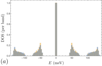
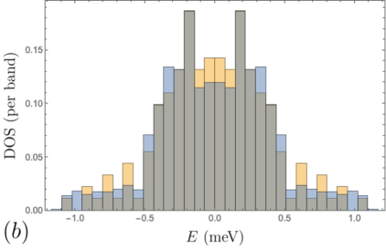
Figure 3: Density of states comparison calculated using the open momentum space method (blue) and exact band structure method (yellow). The overlaps are colored gray. $(a)$ Comparison over the lowest six bands. $(b)$ Zoom in of the flat bands between $\pm 1$meV. In both cases, the agreement is very good. Further improvement can be achieved by increasing the number of momentum space plaquettes in the open momentum space method. In the $84600\times 84600$ matrix, each band has approximately $122$ states [36] (before spurious states are projected out) compared to the band structure technique which we use to compute $1000$ states per band. To achieve convergence between the two densities, more points per band are required.

In Fig. 4, we study the topology of the low lying passive bands. The first important observation is that the passive bands are gapped from each other and the flat bands. This is not the case in zero flux TBG where the first and second passive bands are connected [12] with a Rashba-like dispersion at the $\Gamma$ point [11] due to $C_{3z}$ and $C_{2z}\mathcal{T}$. Recalling Fig. 1b of the Main Text, we see that the first passive bands at $2\pi$ flux (colored red and blue in Fig. 4a) originate from a Landau level which grows linearly in $B$ at small flux. This is exactly what is predicted from the Rashba point discussed in Ref. [11]. As the flux increases, the Landau level degeneracy is broken due to dispersion, acquiring a bandwidth of $\sim 30$meV at $2\pi$ flux. We calculate the Chern number of the bands in Fig. 4b,c and confirm that the first passive bands have $C=-1$, which is the Chern number of a Landau level in our conventions (see Ref. [37] for a direct calculation). We wish to point out an essential difference between the Chern number topology of the flat bands and the Chern numbers of the passive bands. The latter are simply Landau levels (magnetic field induced topology) that have split from the passive bands at $\phi\neq 0$, while the former are a split elementary band representation (crystalline topology) which cannot be described by decoupled Landau levels. Lastly, we calculate the Chern numbers of the second passive bands, and find that they are trivial, i.e. they represent atomic states despite the strong flux. The active bands have Chern number $C=\pm 1$, as the elementary band representation splitting in Eq. 11 of the Main Text shows. Normally, a band with Chern number $C=+1$ can annihilate the topology of a band with $C=-1$ by switching the Chern number in a phase transition. However, in our case, these phase transitions cannot happen: at the high-symmetry momentum $\Gamma$ we have avoided crossings. If the transitions happen at generic points in the band structure, they will happen in pairs (because of $MT$ symmetry), and those pairs come in triplets (because of $C_{3z}$ symmetry), so the Chern number will change by $6$ and this cannot turn the Chern number of the bands to $0$.

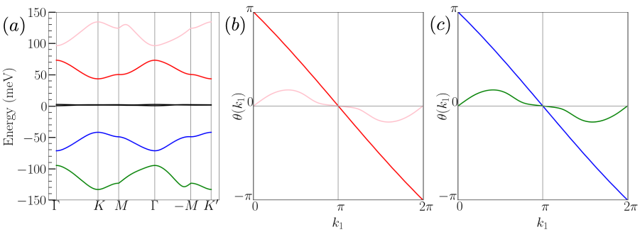
Figure 4: Wilson loops of the passive bands. In $(a)$, we show the $2\pi$ flux band structure at $\theta=1.05^{\circ}$ with the inclusion of particle-hole breaking terms (see App. C). In $(b),(c)$, we compute the Wilson loop over individual bands which are color coded to match $(a)$. We determine from the winding that the first passive passive bands (red and blue) have Chern number $-1$, and the second passive bands (which are gapped) have Chern number 0.

Appendix C Particle-Hole Breaking Terms

In this Appendix, we provide details for incorporating the small angle corrections to the kinetic term of the BM model (Eq. 1 of the Main Text) into the magnetic Bloch Hamiltonian and numerically calculate the Wilson loop. As shown in Sec. III of the Main Text, the band representation $\mathcal{B}$ of the flat bands is a decomposable elementary band representation induced from atomic orbitals. While the two flat bands are connected (as is enforced by $PM\mathcal{T}$), the topology is trivial, as we calculated directly with the Wilson loop. We now show that $O(\theta)$ terms arising from the relative twist in the kinetic term of BM model [12] break the anti-commuting $P$ symmetry, gapping the flat bands are decomposing $\mathcal{B}$ into disconnected bands of opposite Chern number.

To verify this topology numerically, we study the BM Hamiltonian without the particle-hole symmetric approximation. As written in Ref. [15], the Hamiltonian takes the form

$$H_{BM,\theta}=\begin{pmatrix}-iv_{F}(\boldsymbol{\nabla}\cdot\boldsymbol{\sigma}-\frac{\theta}{2}\boldsymbol{\nabla}\times\boldsymbol{\sigma})&T^{\dagger}(\mathbf{r})\\ T(\mathbf{r})&-iv_{F}(\boldsymbol{\nabla}\cdot\boldsymbol{\sigma}+\frac{\theta}{2}\boldsymbol{\nabla}\times\boldsymbol{\sigma}).\end{pmatrix}$$ (22)

which is identical to the expression in Eq. 1 of the Main Text with the addition of the $\pm\frac{\theta}{2}\boldsymbol{\nabla}\times\boldsymbol{\sigma}$ terms which incorporate the opposite rotation of the kinetic terms in the top and bottom layers. Letting $\tau_{i}$ denote Pauli matrices acting on the layer index (which is the matrix notation in Eq. (23)), the additional term is $H_{\theta}\equiv iv_{F}\frac{\theta}{2}\tau_{3}\boldsymbol{\nabla}\times\boldsymbol{\sigma}$. It is direct to see that $H_{\theta}$ breaks particle-hole symmetry $P$ which obeys $PH_{BM}(\mathbf{r})P^{\dagger}=-H_{BM}(\mathbf{r})$. Using the expression for $P=i\tau_{2}R_{\pi}$ where $R_{\pi}$ is the $\pi$ rotation operator on functions (see Ref. [37]), we find that $PH_{\theta}(\mathbf{r})P^{\dagger}=+H_{\theta}(\mathbf{r})$, breaking particle-hole symmetry. We remark that at zero flux, the topology and spectrum of the BM model is not strongly influenced by $P$ because $C_{2z}\mathcal{T}$ ensures the connectedness of the flat bands and protects their topology. The $O(\theta)$ terms which break $P$ at $2\pi$ flux have a more significant effect because $C_{2z}\mathcal{T}$ is also broken, allowing the $O(\theta)$ particle-hole breaking terms to open a gap between the flat bands.

We now discuss the form of $H_{\theta}$ at $2\pi$ flux. We perform the canonical substitution $-i\boldsymbol{\nabla}\rightarrow{\boldsymbol{\pi}}$ to find

$$H_{BM,\theta}^{\phi}(\mathbf{r}) =\begin{pmatrix}v_{F}(\boldsymbol{\pi}\cdot\boldsymbol{\sigma}-\frac{\theta}{2}\boldsymbol{\pi}\times\boldsymbol{\sigma})&T^{\dagger}(\mathbf{r})\\ T(\mathbf{r})&v_{F}(\boldsymbol{\pi}\cdot\boldsymbol{\sigma}+\frac{\theta}{2}\boldsymbol{\pi}\times\boldsymbol{\sigma}).\end{pmatrix}$$ (23)

As written, $H_{BM,\theta}^{\phi}(\mathbf{r})$ is not in Bloch form because $H_{BM,\theta}^{\phi}(\mathbf{r}+\mathbf{a}_{i})\neq H_{BM,\theta}^{\phi}(\mathbf{r})$. To remedy this, we shift into Bloch form via the unitary transformation:

$$V_{1}=\begin{pmatrix}e^{i\pi\mathbf{q}_{1}\cdot\mathbf{r}}&0\\ 0&e^{-i\pi\mathbf{q}_{1}\cdot\mathbf{r}}\end{pmatrix}$$ (24)

which acts as a momentum shift in each layer, reflecting the fact that the Dirac points in the two layers are displaced $2\pi\mathbf{q}_{1}$ from each other. In this section, we only discuss the particle-hole breaking term $H_{\theta}$. All other terms are given explicitly in App. A. We compute

$$V_{1}H_{\theta}^{\phi}V_{1}^{\dagger} =-v_{F}\begin{pmatrix}\frac{\theta}{2}\boldsymbol{\pi}\times\boldsymbol{\sigma}&0\\ 0&-\frac{\theta}{2}\boldsymbol{\pi}\times\boldsymbol{\sigma}.\end{pmatrix}+\pi v_{F}\begin{pmatrix}\frac{\theta}{2}\mathbf{q}_{1}\times\boldsymbol{\sigma}&0\\ 0&\frac{\theta}{2}\mathbf{q}_{1}\times\boldsymbol{\sigma}\end{pmatrix}$$ (25)

$$=-v_{F}\frac{\theta}{2}\tau_{3}\boldsymbol{\pi}\times\boldsymbol{\sigma}+\pi v_{F}\frac{\theta}{2}\tau_{0}\mathbf{q}_{1}\times\boldsymbol{\sigma}\ .$$ (26)

The new term arising from the twist in the kinetic energy is $-v_{F}\frac{\theta}{2}\tau_{3}\boldsymbol{\pi}\times\boldsymbol{\sigma}=-v_{F}\frac{\theta}{2}\tau_{3}(\pi_{x}\sigma_{y}-\pi_{y}\sigma_{x})$. Expanding the $\sigma$ matrices, we get

$$\pi_{x}\sigma_{y}-\pi_{y}\sigma_{x} =\begin{pmatrix}0&-i(\boldsymbol{\pi}_{x}-i\boldsymbol{\pi}_{y})\\ i(\boldsymbol{\pi}_{x}+i\boldsymbol{\pi}_{y})&0\end{pmatrix}=\sqrt{2B}\begin{pmatrix}0&-ia^{\dagger}\\ ia&0\end{pmatrix}$$ (27)

which acts on the sublattice vector indices and the Landau level indices. Making use of $B=\phi/\Omega$ and $\Omega=\frac{2}{3\sqrt{3}}(2\pi/k_{\theta})^{2}$ from Sec. I of the Main Text, we arrive at

$$V_{1}H_{\theta}^{\phi}V_{1}^{\dagger} =\frac{\theta}{2}v_{F}k_{\theta}\sqrt{\dfrac{3\sqrt{3}}{2\pi}}\tau_{z}\otimes\begin{pmatrix}0&ia^{\dagger}\\ -ia&0\end{pmatrix}-\frac{\theta}{4}v_{F}k_{\theta}\tau_{0}\sigma_{x}$$ (28)

where we also use $2\pi\mathbf{q}_{1}\times\boldsymbol{\sigma}=-k_{\theta}\sigma_{x}$. The second term in Eq. (28) acts trivially on the Landau level indices. Both terms in Eq. (28) are smaller than the leading order kinetic term by a factor of $\theta$. Calculating the matrix elements of Eq. (28) on the magnetic translation operator basis states $\ket{\mathbf{k},n,\alpha,l}$ (Eq. 6 of the Main Text), we compute the band structure. As shown in Fig. 5a, the Dirac points at $K$ and $K^{\prime}$ open, leaving the flat bands gapped from each other. We calculate the Wilson loop over each band individually and confirm the $C=\pm 1$ Chern numbers of the split elementary band representation in Fig. 5b. Lastly, we calculate the dispersion of the flat bands over the full BZ in Fig. 5c,d.

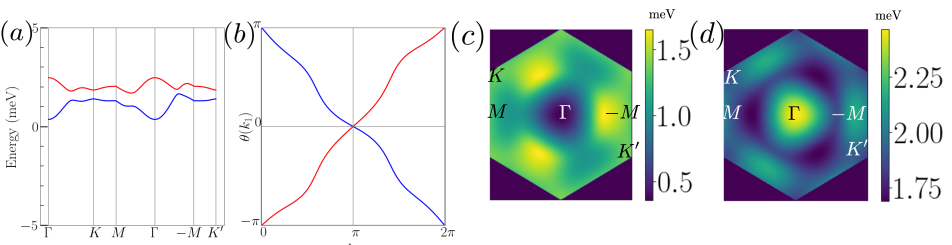
Figure 5: TBG flat bands at $2\pi$ flux with particle-hole breaking terms. $(a)$ Examining the band structure reveals gaps opened at the $K$ and $K^{\prime}$ points, allowing the flat bands to separate. This is only possible in flux when $C_{2z}\mathcal{T}$ is broken. $(b)$ The Abelian Wilson loop, calculated over the two bands separately, reproduces the $C=\pm 1$ Chern numbers predicted from the split elementary band representation. $(c)$ and $(d)$ show the band structure across the BZ of the lower and upper flat bands respectively. The $C_{3z}$ and $M\mathcal{T}$ symmetries are evident in the spectrum.

Appendix D Charge $\pm 1$ Excitation Spectrum

In this section, we give a self-contained derivation of the effective Hamiltonians for charge $\pm 1$ excitations following the method of Ref. [63]. The exact eigenstates $\ket{\Psi_{\nu}}$ defined in the Main Text are amenable to the calculation of various excitation spectra [63]. We describe the simplest case of charge $\pm 1$ excitations, which correspond to adding or removing a single electron from $\ket{\Psi_{\nu}}$. As discussed at length in Ref. [37], the interaction Hamiltonian is

$$H_{int}=\frac{1}{2\Omega_{tot}}\sum_{\mathbf{q}}V(\mathbf{q})\bar{\rho}_{-\mathbf{q}}\bar{\rho}_{\mathbf{q}} =\frac{1}{2\Omega_{tot}}\sum_{\mathbf{G}}\sum_{\mathbf{q}\in BZ}O_{-\mathbf{q},-\mathbf{G}}O_{\mathbf{q},\mathbf{G}},$$ (29)

$$O_{\mathbf{q},\mathbf{G}} =\sqrt{V(\mathbf{q}+2\pi\mathbf{G})}\sum_{\mathbf{k}\in BZ}\sum_{\eta,s}\sum_{MN}\bar{M}^{\eta}_{MN}(\mathbf{k},\mathbf{q}+2\pi\mathbf{G})(\gamma^{\dagger}_{\mathbf{k}-\mathbf{q},M,\eta,s}\gamma_{\mathbf{k},N,\eta,s}-\frac{1}{2}\delta_{MN}\delta_{\mathbf{q},0})$$

where the form factors $M(\mathbf{k},\mathbf{q})$ are defined in Eq. (19). In this Appendix, we find an exact expression for the charge excitations above the groundstate defined in Eq. (14) of the Main Text by

$$\hbox{}[H_{int}-\mu N,\gamma^{\dagger}_{\mathbf{k},M,s,\eta}]\ket{\Psi_{\nu}} \equiv\frac{1}{2}\sum_{N}\gamma^{\dagger}_{\mathbf{k},N,s,\eta}[R^{\eta}_{+}(\mathbf{k})]_{NM}\ket{\Psi_{\nu}}$$ (30)

where $-\mu N$ is the chemical potential term obeying $[N,\gamma^{\dagger}_{\mathbf{k},M,s,\eta}]=\gamma^{\dagger}_{\mathbf{k},M,s,\eta}$. To compute the $[H_{int},\gamma^{\dagger}_{\mathbf{k},M,s,\eta}]$ we first need the commutators

$$\hbox{}[O_{\mathbf{q},\mathbf{G}},\gamma^{\dagger}_{\mathbf{k},M,s,\eta}] =\sqrt{V(\mathbf{q}+2\pi\mathbf{G})}\sum_{N}\gamma^{\dagger}_{\mathbf{k}-\mathbf{q},N,\eta,s}\bar{M}^{\eta}_{NM}(\mathbf{k},\mathbf{q}+2\pi\mathbf{G})$$ (31)

$$\hbox{}[O_{\mathbf{q},\mathbf{G}},\gamma_{\mathbf{k},M,s,\eta}] =-[O_{-\mathbf{q},-\mathbf{G}},\gamma^{\dagger}_{\mathbf{k},M,s,\eta}]^{\dagger}=-\sqrt{V(\mathbf{q}+2\pi\mathbf{G})}\sum_{N}\gamma_{\mathbf{k}+\mathbf{q},N,\eta,s}\bar{M^{\eta}}^{*}_{NM}(\mathbf{k},-\mathbf{q}-2\pi\mathbf{G})\ .$$

We will focus on the charge $+1$ excitations which arises from the $\gamma^{\dagger}_{\mathbf{k},M,s,\eta}$ commutator. Analogous formulae for the $-1$ excitations can be obtained from the $\gamma_{\mathbf{k},M,s,\eta}$. Using Eq. (31), we calculate

$$\hbox{}[O_{-\mathbf{q},-\mathbf{G}}O_{\mathbf{q},\mathbf{G}},\gamma^{\dagger}_{\mathbf{k},M,s,\eta}] =O_{-\mathbf{q},-\mathbf{G}}[O_{\mathbf{q},\mathbf{G}},\gamma^{\dagger}_{\mathbf{k},M,s,\eta}]+[O_{-\mathbf{q},-\mathbf{G}},\gamma^{\dagger}_{\mathbf{k},M,s,\eta}]O_{\mathbf{q},\mathbf{G}}$$ (32)

$$=\sqrt{V(\mathbf{q}+2\pi\mathbf{G})}\sum_{N}O_{-\mathbf{q},-\mathbf{G}}\gamma^{\dagger}_{\mathbf{k}-\mathbf{q},N,\eta,s}\bar{M}^{\eta}_{NM}(\mathbf{k},\mathbf{q}+2\pi\mathbf{G})$$

$$\qquad+\sqrt{V(\mathbf{q}+2\pi\mathbf{G})}\sum_{N}\gamma^{\dagger}_{\mathbf{k}+\mathbf{q},N,\eta,s}\bar{M}^{\eta}_{NM}(\mathbf{k},-\mathbf{q}-2\pi\mathbf{G})O_{\mathbf{q},\mathbf{G}}$$

$$=\sqrt{V(\mathbf{q}+2\pi\mathbf{G})}\sum_{N}(\gamma^{\dagger}_{\mathbf{k}-\mathbf{q},N,\eta,s}O_{-\mathbf{q},-\mathbf{G}}-[\gamma^{\dagger}_{\mathbf{k}-\mathbf{q},N,\eta,s},O_{-\mathbf{q},-\mathbf{G}}])\bar{M}^{\eta}_{NM}(\mathbf{k},\mathbf{q}+2\pi\mathbf{G})$$

$$\qquad+\sqrt{V(\mathbf{q}+2\pi\mathbf{G})}\sum_{N}\gamma^{\dagger}_{\mathbf{k}+\mathbf{q},N,\eta,s}\bar{M}^{\eta}_{NM}(\mathbf{k},-\mathbf{q}-2\pi\mathbf{G})O_{\mathbf{q},\mathbf{G}}$$

Evaluating the remaining commutator, we find

$$\hbox{}[O_{-\mathbf{q},-\mathbf{G}}O_{\mathbf{q},\mathbf{G}},\gamma^{\dagger}_{\mathbf{k},M,s,\eta}] =V(\mathbf{q}+2\pi\mathbf{G})\sum_{N}\gamma^{\dagger}_{\mathbf{k},N,\eta,s}[\bar{M}^{\eta}(\mathbf{k}-\mathbf{q}-2\pi\mathbf{G},-\mathbf{q}-2\pi\mathbf{G})\bar{M}^{\eta}(\mathbf{k},\mathbf{q}+2\pi\mathbf{G})]_{NM}$$ (33)

$$\qquad+\sqrt{V(\mathbf{q}+2\pi\mathbf{G})}\sum_{N}\left(\gamma^{\dagger}_{\mathbf{k}+\mathbf{q},N,\eta,s}\bar{M}^{\eta}_{NM}(\mathbf{k},-\mathbf{q}-2\pi\mathbf{G})O_{\mathbf{q},\mathbf{G}}+\gamma^{\dagger}_{\mathbf{k}-\mathbf{q},N,\eta,s}\bar{M}^{\eta}_{NM}(\mathbf{k},\mathbf{q}+2\pi\mathbf{G})O_{-\mathbf{q},-\mathbf{G}}\right)\ .$$

Let us focus on the form factor product $\bar{M}(\mathbf{k}-\mathbf{q},-\mathbf{q})\bar{M}(\mathbf{k},\mathbf{q})$. Using Eq. (19), we compute (suppressing the $\eta$ index temporarily)

$$\bar{M}(\mathbf{k}-\mathbf{q},-\mathbf{q})\bar{M}(\mathbf{k},\mathbf{q}) =e^{i\xi_{\mathbf{q}}(\mathbf{k})+i\xi_{-\mathbf{q}}(\mathbf{k}-\mathbf{q})}U^{\dagger}(\mathbf{k})\mathcal{H}^{-\mathbf{q}}U(\mathbf{k}-\mathbf{q})U^{\dagger}(\mathbf{k}-\mathbf{q})\mathcal{H}^{\mathbf{q}}U(\mathbf{k})$$ (34)

$$=U^{\dagger}(\mathbf{k})\mathcal{H}^{-\mathbf{q}}U(\mathbf{k}-\mathbf{q})U^{\dagger}(\mathbf{k}-\mathbf{q})\mathcal{H}^{\mathbf{q}}U(\mathbf{k})$$

$$=(U^{\dagger}(\mathbf{k}-\mathbf{q})\mathcal{H}^{\mathbf{q}}U(\mathbf{k}))^{\dagger}\,U^{\dagger}(\mathbf{k}-\mathbf{q})\mathcal{H}^{\mathbf{q}}U(\mathbf{k})$$

$$=M^{\dagger}(\mathbf{k},\mathbf{q})M(\mathbf{k},\mathbf{q})\equiv P(\mathbf{k},\mathbf{q})$$

where we used the identity $e^{-i\xi_{\mathbf{q}}(\mathbf{k})-i\xi_{-\mathbf{q}}(\mathbf{k}-\mathbf{q})}=1$ proven in Ref. [37] and $\mathcal{H}^{-\mathbf{q}}={\mathcal{H}^{\mathbf{q}}}^{\dagger}$. As a result of Eq. (34),

$$P^{\eta}(\mathbf{k},\mathbf{q}+2\pi\mathbf{G})\equiv{M^{\eta}}^{\dagger}(\mathbf{k},\mathbf{q}+2\pi\mathbf{G})M^{\eta}(\mathbf{k},\mathbf{q}+2\pi\mathbf{G})$$ (35)

is positive semi-definite. The second line of Eq. (33) simplifies considerably when acting on $\ket{\Psi_{\nu}}$ (defined in Eq. (13) of the Main Text):

$$O_{\mathbf{q},\mathbf{G}}\ket{\Psi_{\nu}} =\delta_{\mathbf{q},0}\sqrt{V(2\pi\mathbf{G})}\sum_{\mathbf{k}\in BZ}\sum_{\eta,s}\sum_{MN}\bar{M}^{\eta}_{MN}(\mathbf{k},2\pi\mathbf{G})(\gamma^{\dagger}_{\mathbf{k},M,\eta,s}\gamma_{\mathbf{k},N,\eta,s}-\frac{1}{2}\delta_{MN})\ket{\Psi_{\nu}}$$ (36)

$$=\delta_{\mathbf{q},0}\sqrt{V(2\pi\mathbf{G})}\sum_{\mathbf{k}\in BZ}\sum_{\eta,s}(\sum_{j}\delta_{s,s_{j}}\delta_{\eta,\eta_{j}}\text{Tr}\ [\bar{M}^{\eta}(\mathbf{k},2\pi\mathbf{G})]-\frac{1}{2}\text{Tr}\ [\bar{M}^{\eta}(\mathbf{k},2\pi\mathbf{G})])\ket{\Psi_{\nu}}$$

$$=\delta_{\mathbf{q},0}\sqrt{V(2\pi\mathbf{G})}\sum_{\mathbf{k}\in BZ}(\frac{\nu+4}{2}\text{Tr}\ [\bar{M}^{\eta}(\mathbf{k},2\pi\mathbf{G})]-\frac{4}{2}\text{Tr}\ [\bar{M}^{\eta}(\mathbf{k},2\pi\mathbf{G})])\ket{\Psi_{\nu}}$$

$$=\nu\delta_{\mathbf{q},0}\sqrt{V(2\pi\mathbf{G})}\sum_{\mathbf{k}\in BZ}\frac{1}{2}\text{Tr}\ \bar{M}^{\eta}(\mathbf{k},2\pi\mathbf{G})\ket{\Psi_{\nu}}\ .$$

Returning to the second line of Eq. (33) and using Eq. (36), we obtain:

$$\sqrt{V(\mathbf{q}+2\pi\mathbf{G})}\sum_{N}\left(\gamma^{\dagger}_{\mathbf{k}+\mathbf{q},N,\eta,s}\bar{M}_{NM}(\mathbf{k},-\mathbf{q}-2\pi\mathbf{G})O_{\mathbf{q},\mathbf{G}}+\gamma^{\dagger}_{\mathbf{k}-\mathbf{q},N,\eta,s}\bar{M}_{NM}(\mathbf{k},\mathbf{q}+2\pi\mathbf{G})O_{-\mathbf{q},-\mathbf{G}}\right)\ket{\Psi_{\nu}}$$ (37)

$$=\nu\delta_{\mathbf{q},0}V(2\pi\mathbf{G})\left(\sum_{\mathbf{q}^{\prime}\in BZ}\frac{1}{2}\text{Tr}\ \bar{M}(\mathbf{q},2\pi\mathbf{G})\right)\sum_{N}\gamma^{\dagger}_{\mathbf{k},N,\eta,s}\left(\bar{M}_{NM}(\mathbf{k},-2\pi\mathbf{G})+\bar{M}_{NM}(\mathbf{k},2\pi\mathbf{G})\right)\ket{\Psi_{\nu}}\ .$$

The sum $[\bar{M}(\mathbf{k},-2\pi\mathbf{G})+\bar{M}(\mathbf{k},2\pi\mathbf{G})]_{NM}$ is Hermitian, which it must be because this term is part of the effective Hamiltonian. Gathering results, we find the effective Hamiltonian $\frac{1}{2}R^{\eta}_{\pm}(\mathbf{k})$ where $R^{\eta}_{+}(\mathbf{k})=R^{\eta}_{F}(\mathbf{k})+\nu R^{\eta}_{H}(\mathbf{k})-2\mu\mathbb{1}$ and $R^{\eta}_{-}(\mathbf{k})^{*}=R^{\eta}_{F}(\mathbf{k})-\nu R^{\eta}_{H}(\mathbf{k})+2\mu\mathbb{1}$ and the various terms are defined by

$$R^{\eta}_{F}(\mathbf{k}) =\sum_{\mathbf{G}}\left(\frac{1}{N_{M}}\sum_{\mathbf{q}\in BZ}\Omega^{-1}V(\mathbf{q}+2\pi\mathbf{G}){M^{\eta}}^{\dagger}(\mathbf{k},\mathbf{q}+2\pi\mathbf{G})M^{\eta}(\mathbf{k},\mathbf{q}+2\pi\mathbf{G})\right),$$ (38)

$$R^{\eta}_{H}(\mathbf{k}) =\sum_{\mathbf{G}\neq 0}\Omega^{-1}V(2\pi\mathbf{G})\left(\frac{1}{N_{M}}\sum_{\mathbf{q}\in BZ}\frac{1}{2}\text{Tr}\ M^{\eta}(\mathbf{q},2\pi\mathbf{G})\right)M^{\eta}(\mathbf{k},2\pi\mathbf{G})+H.c.,$$

$$\mu =\nu\sum_{\mathbf{G}\neq 0}\Omega^{-1}V(2\pi\mathbf{G})\left(\frac{1}{N_{M}}\sum_{\mathbf{q}\in BZ}\frac{1}{2}\text{Tr}\ M^{\eta}(\mathbf{q},2\pi\mathbf{G})\right)^{2}\$$

where we have discretized the Brillouin zone by taking $N_{M}$ to be the (finite) number of moiré unit cells, so each $\mathbf{q}$ sum has $N_{M}$ terms. The value of the chemical potential is derived using the flat metric approximation in Ref. [37]. Importantly, the Fock term $R_{F}(\mathbf{k})$ is positive definite [61]. We conclude that the groundstate $\ket{\Psi_{0}}$ where $\nu=0$ is stable to charge excitations and generically (but not always) will be insulating. Lastly, we note that

$$R^{-\eta}_{F}(\mathbf{k}) =\nu_{1}R^{\eta}_{F}(\mathbf{k})\nu_{1},\qquad R^{-\eta}_{H}(\mathbf{k})=\nu_{1}R^{\eta}_{H}(\mathbf{k})\nu_{1}$$ (39)

where $\nu_{1}$ is a Pauli matrix, so charge $+1$ and charge $-1$ spectra are related by the unitary matrix $\nu_{1}$ and hence have identical spectra.

In Fig. 6, we study the dispersion relation of the quasi-particles near $\nu=0$ obtained from the charge $\pm 1$ excitation Hamiltonian $R^{\eta}_{\pm}(\mathbf{k})$. We find that the nearly degenerate bands at the $\Gamma$ point for $w_{0}/w_{1}=.8$ (shown in Fig. 2 of the Main Text) are not generic, which is understood from the symmetries. At zero flux, Ref. [61] found that the excitation bands had a protected degeneracy at the $\Gamma$ point due to $C_{2z}\mathcal{T}$ symmetry, but nonzero flux breaks this symmetry and allows the bands to gap. Fig. 6a shows the gap between the two excitation bands at $\Gamma$ as a function of $w_{0}$, from which we see that $w_{0}=.8w_{1}$ is in a non-generic region in the parameter space where the bands are close in energy. Fig. 6b-d show three examples of excitation band structures.

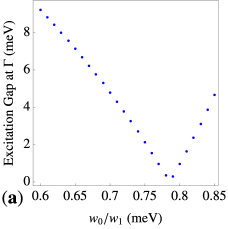
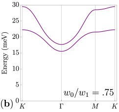
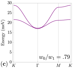
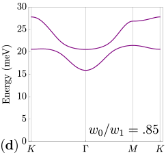
Figure 6: Charge $\pm 1$ excitations at $\nu=0$ using $\xi=10$nm in Eq. (18). $(a)$ The excitation gap of $R^{\eta}_{\pm}(\mathbf{k}=0)$ is plotted as a function of $w_{0}$, showing that the near-degeneracy of the bands at $w_{0}/w_{1}=.8$ is accidental. $(b)-(d)$ display the band structure at $w_{0}/w_{1}=.75,.79,.85$ respectively, highlighting the gap closing and reopening at $\Gamma$ as $w_{0}/w_{1}$ is increased.

References

- Cao et al. (2018) Yuan Cao, Valla Fatemi, Ahmet Demir, Shiang Fang, Spencer L. Tomarken, Jason Y. Luo, Javier D. Sanchez-Yamagishi, Kenji Watanabe, Takashi Taniguchi, Efthimios Kaxiras, Ray C. Ashoori, and Pablo Jarillo-Herrero. Correlated insulator behaviour at half-filling in magic-angle graphene superlattices. Nature (London), 556(7699):80–84, Apr 2018. doi: 10.1038/nature26154.
- Cao et al. (2018) Yuan Cao, V. Fatemi, S. Fang, K. Watanabe, T. Taniguchi, E. Kaxiras, and P. Jarillo-Herrero. Unconventional superconductivity in magic-angle graphene superlattices. Nature, 556:43–50, 2018.
- Kim et al. (2017) Kyounghwan Kim, Ashley DaSilva, Shengqiang Huang, Babak Fallahazad, Stefano Larentis, Takashi Taniguchi, Kenji Watanabe, Brian J. LeRoy, Allan H. MacDonald, and Emanuel Tutuc. Tunable moiré bands and strong correlations in small-twist-angle bilayer graphene. Proceedings of the National Academy of Sciences, 114(13):3364–3369, 2017. ISSN 0027-8424. doi: 10.1073/pnas.1620140114. URL https://www.pnas.org/content/114/13/3364.
- Kennes et al. (2021) Dante M. Kennes, Martin Claassen, Lede Xian, Antoine Georges, Andrew J. Millis, James Hone, Cory R. Dean, D. N. Basov, Abhay N. Pasupathy, and Angel Rubio. Moiré heterostructures as a condensed-matter quantum simulator. Nature Physics, 17(2):155–163, January 2021. doi: 10.1038/s41567-020-01154-3.
- Balents et al. (2020) Leon Balents, Cory R Dean, Dmitri K Efetov, and Andrea F Young. Superconductivity and strong correlations in moiré flat bands. Nature Physics, 16(7):725–733, 2020.
- Liu and Dai (2021) Jianpeng Liu and Xi Dai. Orbital magnetic states in moiré graphene systems. Nature Reviews Physics, pages 1–16, 2021.
- Chu et al. (2020) Yanbang Chu, Le Liu, Yalong Yuan, Cheng Shen, Rong Yang, Dongxia Shi, Wei Yang, and Guangyu Zhang. A review of experimental advances in twisted graphene moiré superlattice. Chinese Physics B, 29(12):128104, dec 2020. doi: 10.1088/1674-1056/abb221. URL https://doi.org/10.1088/1674-1056/abb221.
- Herzog-Arbeitman et al. (2020) Jonah Herzog-Arbeitman, Zhi-Da Song, Nicolas Regnault, and B. Andrei Bernevig. Hofstadter topology: Noncrystalline topological materials at high flux. Phys. Rev. Lett., 125:236804, Dec 2020. doi: 10.1103/PhysRevLett.125.236804. URL https://link.aps.org/doi/10.1103/PhysRevLett.125.236804.
- Bistritzer and MacDonald (2011) Rafi Bistritzer and Allan H. MacDonald. Moiré bands in twisted double-layer graphene. Proceedings of the National Academy of Science, 108(30):12233–12237, Jul 2011. doi: 10.1073/pnas.1108174108.
- Koshino et al. (2018) Mikito Koshino, Noah F. Q. Yuan, Takashi Koretsune, Masayuki Ochi, Kazuhiko Kuroki, and Liang Fu. Maximally localized wannier orbitals and the extended hubbard model for twisted bilayer graphene. Phys. Rev. X, 8:031087, Sep 2018. doi: 10.1103/PhysRevX.8.031087. URL https://link.aps.org/doi/10.1103/PhysRevX.8.031087.
- Das et al. (2021) Ipsita Das, Xiaobo Lu, Jonah Herzog-Arbeitman, Zhi-Da Song, Kenji Watanabe, Takashi Taniguchi, B. Andrei Bernevig, and Dmitri K. Efetov. Symmetry-broken Chern insulators and Rashba-like Landau-level crossings in magic-angle bilayer graphene. Nature Physics, 17(6):710–714, January 2021. doi: 10.1038/s41567-021-01186-3.
- Song et al. (2019) Zhi-Da Song, Zhijun Wang, Wujun Shi, Gang Li, Chen Fang, and B. Andrei Bernevig. All Magic Angles in Twisted Bilayer Graphene are Topological. Phys. Rev. Lett. , 123(3):036401, Jul 2019. doi: 10.1103/PhysRevLett.123.036401.
- Tarnopolsky et al. (2019) Grigory Tarnopolsky, Alex Jura Kruchkov, and Ashvin Vishwanath. Origin of magic angles in twisted bilayer graphene. Phys. Rev. Lett., 122:106405, Mar 2019. doi: 10.1103/PhysRevLett.122.106405. URL https://link.aps.org/doi/10.1103/PhysRevLett.122.106405.
- Bernevig et al. (2021a) B. Andrei Bernevig, Zhi-Da Song, Nicolas Regnault, and Biao Lian. Twisted bilayer graphene. I. Matrix elements, approximations, perturbation theory, and a k .p two-band model. Phys. Rev. B, 103(20):205411, May 2021a. doi: 10.1103/PhysRevB.103.205411.
- Song et al. (2021) Zhi-Da Song, Biao Lian, Nicolas Regnault, and B. Andrei Bernevig. Twisted bilayer graphene. II. Stable symmetry anomaly. Phys. Rev. B, 103(20):205412, May 2021. doi: 10.1103/PhysRevB.103.205412.
- Wang et al. (2020) Jie Wang, Yunqin Zheng, Andrew J. Millis, and Jennifer Cano. Chiral Approximation to Twisted Bilayer Graphene: Exact Intra-Valley Inversion Symmetry, Nodal Structure and Implications for Higher Magic Angles. arXiv e-prints, art. arXiv:2010.03589, October 2020.
- Chen et al. (2020) Bin-Bin Chen, Yuan Da Liao, Ziyu Chen, Oskar Vafek, Jian Kang, Wei Li, and Zi Yang Meng. Realization of Topological Mott Insulator in a Twisted Bilayer Graphene Lattice Model. arXiv e-prints, art. arXiv:2011.07602, November 2020.
- Zou et al. (2018) Liujun Zou, Hoi Chun Po, Ashvin Vishwanath, and T. Senthil. Band structure of twisted bilayer graphene: Emergent symmetries, commensurate approximants, and wannier obstructions. Phys. Rev. B, 98:085435, Aug 2018. doi: 10.1103/PhysRevB.98.085435. URL https://link.aps.org/doi/10.1103/PhysRevB.98.085435.
- Hofstadter (1976) Douglas R. Hofstadter. Energy levels and wave functions of bloch electrons in rational and irrational magnetic fields. Phys. Rev. B, 14:2239–2249, Sep 1976. doi: 10.1103/PhysRevB.14.2239.
- Wang and Santos (2020) Jian Wang and Luiz H. Santos. Classification of topological phase transitions and van hove singularity steering mechanism in graphene superlattices. Phys. Rev. Lett., 125:236805, Dec 2020. doi: 10.1103/PhysRevLett.125.236805. URL https://link.aps.org/doi/10.1103/PhysRevLett.125.236805.
- Albrecht et al. (2001) C. Albrecht, J. H. Smet, K. von Klitzing, D. Weiss, V. Umansky, and H. Schweizer. Evidence of hofstadter’s fractal energy spectrum in the quantized hall conductance. Phys. Rev. Lett., 86:147–150, Jan 2001. doi: 10.1103/PhysRevLett.86.147. URL https://link.aps.org/doi/10.1103/PhysRevLett.86.147.
- Bernevig and Hughes (2013) B. Andrei Bernevig and Taylor L. Hughes. Topological Insulators and Topological Superconductors. Princeton University Press, student edition edition, 2013. ISBN 9780691151755.
- Lu et al. (2020) Xiaobo Lu, Biao Lian, Gaurav Chaudhary, Benjamin A. Piot, Giulio Romagnoli, Kenji Watanabe, Takashi Taniguchi, Martino Poggio, Allan H. MacDonald, B. Andrei Bernevig, and Dmitri K. Efetov. Fingerprints of Fragile Topology in the Hofstadter spectrum of Twisted Bilayer Graphene Close to the Second Magic Angle. PNAS, art. arXiv:2006.13963, June 2020.
- Dean et al. (2013) C. R. Dean, L. Wang, P. Maher, C. Forsythe, F. Ghahari, Y. Gao, J. Katoch, M. Ishigami, P. Moon, M. Koshino, T. Taniguchi, K. Watanabe, K. L. Shepard, J. Hone, and P. Kim. Hofstadter’s butterfly and the fractal quantum hall effect in moirésuperlattices. Nature, 497:598 EP –, 05 2013.
- Zak (1964a) J. Zak. Magnetic translation group. Phys. Rev., 134:A1602–A1606, Jun 1964a. doi: 10.1103/PhysRev.134.A1602. URL https://link.aps.org/doi/10.1103/PhysRev.134.A1602.
- Zak (1964b) J. Zak. Magnetic translation group. ii. irreducible representations. Phys. Rev., 134:A1607–A1611, Jun 1964b. doi: 10.1103/PhysRev.134.A1607. URL https://link.aps.org/doi/10.1103/PhysRev.134.A1607.
- Brown (1969) E. Brown. Aspects of group theory in electron dynamics**this work supported by the u.s. atomic energy commission. 22:313–408, 1969. ISSN 0081-1947. doi: https://doi.org/10.1016/S0081-1947(08)60033-8. URL https://www.sciencedirect.com/science/article/pii/S0081194708600338.
- Streda (1982) P Streda. Theory of quantised hall conductivity in two dimensions. Journal of Physics C: Solid State Physics, 15(22):L717–L721, aug 1982. doi: 10.1088/0022-3719/15/22/005. URL https://doi.org/10.1088/0022-3719/15/22/005.
- Wannier (1978) G. H. Wannier. A Result Not Dependent on Rationality for Bloch Electrons in a Magnetic Field. Physica Status Solidi B Basic Research, 88(2):757–765, August 1978. doi: 10.1002/pssb.2220880243.
- Pereira et al. (2007) J. Milton Pereira, F. M. Peeters, and P. Vasilopoulos. Landau levels and oscillator strength in a biased bilayer of graphene. Phys. Rev. B, 76:115419, Sep 2007. doi: 10.1103/PhysRevB.76.115419. URL https://link.aps.org/doi/10.1103/PhysRevB.76.115419.
- Xiao et al. (2010) Di Xiao, Ming-Che Chang, and Qian Niu. Berry phase effects on electronic properties. Rev. Mod. Phys., 82:1959–2007, Jul 2010. doi: 10.1103/RevModPhys.82.1959. URL https://link.aps.org/doi/10.1103/RevModPhys.82.1959.
- Gumbs et al. (1995) Godfrey Gumbs, Desiré Miessein, and Danhong Huang. Effect of magnetic modulation on bloch electrons on a two-dimensional square lattice. Phys. Rev. B, 52:14755–14760, Nov 1995. doi: 10.1103/PhysRevB.52.14755. URL https://link.aps.org/doi/10.1103/PhysRevB.52.14755.
- Bistritzer and MacDonald (2011) R. Bistritzer and A. H. MacDonald. Moiré butterflies in twisted bilayer graphene. Phys. Rev. B, 84:035440, Jul 2011. doi: 10.1103/PhysRevB.84.035440. URL https://link.aps.org/doi/10.1103/PhysRevB.84.035440.
- Hejazi et al. (2019) Kasra Hejazi, Chunxiao Liu, and Leon Balents. Landau levels in twisted bilayer graphene and semiclassical orbits. Phys. Rev. B, 100(3):035115, July 2019. doi: 10.1103/PhysRevB.100.035115.
- Crosse et al. (2020) J. A. Crosse, Naoto Nakatsuji, Mikito Koshino, and Pilkyung Moon. Hofstadter butterfly and the quantum hall effect in twisted double bilayer graphene. Physical Review B, 102(3), Jul 2020. ISSN 2469-9969. doi: 10.1103/physrevb.102.035421. URL http://dx.doi.org/10.1103/PhysRevB.102.035421.
- Lian et al. (2021a) Biao Lian, Fang Xie, and B. Andrei Bernevig. Open momentum space method for the Hofstadter butterfly and the quantized Lorentz susceptibility. Phys. Rev. B, 103(16):L161405, April 2021a. doi: 10.1103/PhysRevB.103.L161405.
- (37) Jonah Herzog-Arbeitman, Aaron Chew, and Andrei Bernevig. The magnetic bloch theorem at flux.
- (38) Ipsita Das, Cheng Shen, Alexandre Jaoui, Jonah Herzog-Arbeitman, Aaron Chew, Chang-Woo Cho, Kenji Watanabe, Takashi Taniguchi, Benjamin A. Piot, B. Andrei Bernevig, and Dmitri K. Efetov. Observation of re-entrant correlated insulators and interaction driven fermi surface reconstructions at one magnetic flux quantum per moiré unit cell in magic-angle twisted bilayer graphene.
- Brouder et al. (2007) Christian Brouder, Gianluca Panati, Matteo Calandra, Christophe Mourougane, and Nicola Marzari. Exponential localization of wannier functions in insulators. Physical Review Letters, 98(4), Jan 2007. ISSN 1079-7114. doi: 10.1103/physrevlett.98.046402.
- Alexandradinata et al. (2014) A. Alexandradinata, Xi Dai, and B. Andrei Bernevig. Wilson-Loop Characterization of Inversion-Symmetric Topological Insulators. Phys. Rev., B89(15):155114, 2014. doi: 10.1103/PhysRevB.89.155114.
- Bradlyn et al. (2017) Barry Bradlyn, L. Elcoro, Jennifer Cano, M. G. Vergniory, Zhijun Wang, C. Felser, M. I. Aroyo, and B. Andrei Bernevig. Topological quantum chemistry. Nature (London), 547(7663):298–305, Jul 2017. doi: 10.1038/nature23268.
- Aroyo et al. (2006a) MI Aroyo, JM Perez-Mato, Cesar Capillas, Eli Kroumova, Svetoslav Ivantchev, Gotzon Madariaga, Asen Kirov, and Hans Wondratschek. Bilbao crystallographic server: I. databases and crystallographic computing programs. ZEITSCHRIFT FUR KRISTALLOGRAPHIE, 221:15–27, 01 2006a. doi: 10.1524/zkri.2006.221.1.15.
- Aroyo et al. (2006b) Mois I. Aroyo, Asen Kirov, Cesar Capillas, J. M. Perez-Mato, and Hans Wondratschek. Bilbao Crystallographic Server. II. Representations of crystallographic point groups and space groups. Acta Crystallographica Section A, 62(2):115–128, Mar 2006b. doi: 10.1107/S0108767305040286.
- Kang and Vafek (2018) Jian Kang and Oskar Vafek. Symmetry, Maximally Localized Wannier States, and a Low-Energy Model for Twisted Bilayer Graphene Narrow Bands. Physical Review X, 8(3):031088, July 2018. doi: 10.1103/PhysRevX.8.031088.
- Cano et al. (2018a) Jennifer Cano, Barry Bradlyn, Zhijun Wang, L. Elcoro, M. G. Vergniory, C. Felser, M. I. Aroyo, and B. Andrei Bernevig. Topology of Disconnected Elementary Band Representations. Phys. Rev. Lett. , 120(26):266401, June 2018a. doi: 10.1103/PhysRevLett.120.266401.
- Cano et al. (2018b) Jennifer Cano, Barry Bradlyn, Zhijun Wang, L. Elcoro, M. G. Vergniory, C. Felser, M. I. Aroyo, and B. Andrei Bernevig. Building blocks of topological quantum chemistry: Elementary band representations. Phys. Rev. B, 97(3):035139, Jan 2018b. doi: 10.1103/PhysRevB.97.035139.
- Bradlyn et al. (2019) Barry Bradlyn, Zhijun Wang, Jennifer Cano, and B. Andrei Bernevig. Disconnected elementary band representations, fragile topology, and wilson loops as topological indices: An example on the triangular lattice. Physical Review B, 99(4), Jan 2019. ISSN 2469-9969. doi: 10.1103/physrevb.99.045140. URL http://dx.doi.org/10.1103/PhysRevB.99.045140.
- Fang et al. (2012) Chen Fang, Matthew J. Gilbert, and B. Andrei Bernevig. Bulk topological invariants in noninteracting point group symmetric insulators. Phys. Rev. B, 86(11):115112, September 2012. doi: 10.1103/PhysRevB.86.115112.
- Liu et al. (2019) Jianpeng Liu, Junwei Liu, and Xi Dai. Pseudo landau level representation of twisted bilayer graphene: Band topology and implications on the correlated insulating phase. Phys. Rev. B, 99:155415, Apr 2019. doi: 10.1103/PhysRevB.99.155415. URL https://link.aps.org/doi/10.1103/PhysRevB.99.155415.
- Ahn et al. (2019) J. Ahn, S. Park, and B.-J. Yang. Failure of Nielsen-Ninomiya Theorem and Fragile Topology in Two-Dimensional Systems with Space-Time Inversion Symmetry: Application to Twisted Bilayer Graphene at Magic Angle. Physical Review X, 9(2):021013, April 2019. doi: 10.1103/PhysRevX.9.021013.
- Bernevig et al. (2021b) B. Andrei Bernevig, Zhi-Da Song, Nicolas Regnault, and Biao Lian. Twisted bilayer graphene. III. Interacting Hamiltonian and exact symmetries. Phys. Rev. B, 103(20):205413, May 2021b. doi: 10.1103/PhysRevB.103.205413.
- Liu et al. (2021) Xiaoxue Liu, Zhi Wang, K. Watanabe, T. Taniguchi, Oskar Vafek, and J. I. A. Li. Tuning electron correlation in magic-angle twisted bilayer graphene using Coulomb screening. Science, 371(6535):1261–1265, March 2021. doi: 10.1126/science.abb8754.
- Vafek and Kang (2020) Oskar Vafek and Jian Kang. Towards the hidden symmetry in Coulomb interacting twisted bilayer graphene: renormalization group approach. arXiv e-prints, art. arXiv:2009.09413, September 2020.
- Wilson et al. (2020) Justin H. Wilson, Yixing Fu, S. Das Sarma, and J. H. Pixley. Disorder in twisted bilayer graphene. Phys. Rev. Research, 2:023325, Jun 2020. doi: 10.1103/PhysRevResearch.2.023325. URL https://link.aps.org/doi/10.1103/PhysRevResearch.2.023325.
- Parker et al. (2020) Daniel E. Parker, Tomohiro Soejima, Johannes Hauschild, Michael P. Zaletel, and Nick Bultinck. Strain-induced quantum phase transitions in magic angle graphene. arXiv e-prints, art. arXiv:2012.09885, December 2020.
- Padhi et al. (2020) Bikash Padhi, Apoorv Tiwari, Titus Neupert, and Shinsei Ryu. Transport across twist angle domains in moiré graphene. arXiv e-prints, art. arXiv:2005.02406, May 2020.
- Uri et al. (2020) A. Uri, S. Grover, Y. Cao, J. Â. A. Crosse, K. Bagani, D. Rodan-Legrain, Y. Myasoedov, K. Watanabe, T. Taniguchi, P. Moon, M. Koshino, P. Jarillo-Herrero, and E. Zeldov. Mapping the twist-angle disorder and Landau levels in magic-angle graphene. Nature (London), 581(7806):47–52, May 2020. doi: 10.1038/s41586-020-2255-3.
- Kazmierczak et al. (2020) Nathanael P. Kazmierczak, Madeline Van Winkle, Colin Ophus, Karen C. Bustillo, Hamish G. Brown, Stephen Carr, Jim Ciston, Takashi Taniguchi, Kenji Watanabe, and D. Kwabena Bediako. Strain fields in twisted bilayer graphene. arXiv e-prints, art. arXiv:2008.09761, August 2020.
- Benschop et al. (2021) Tjerk Benschop, Tobias A. de Jong, Petr Stepanov, Xiaobo Lu, Vincent Stalman, Sense Jan van der Molen, Dmitri K. Efetov, and Milan P. Allan. Measuring local moiré lattice heterogeneity of twisted bilayer graphene. Phys. Rev. Research, 3:013153, Feb 2021. doi: 10.1103/PhysRevResearch.3.013153. URL https://link.aps.org/doi/10.1103/PhysRevResearch.3.013153.
- Kang and Vafek (2019) Jian Kang and Oskar Vafek. Strong coupling phases of partially filled twisted bilayer graphene narrow bands. Phys. Rev. Lett., 122:246401, Jun 2019. doi: 10.1103/PhysRevLett.122.246401. URL https://link.aps.org/doi/10.1103/PhysRevLett.122.246401.
- Bernevig et al. (2021c) B. Andrei Bernevig, Biao Lian, Aditya Cowsik, Fang Xie, Nicolas Regnault, and Zhi-Da Song. Twisted bilayer graphene. V. Exact analytic many-body excitations in Coulomb Hamiltonians: Charge gap, Goldstone modes, and absence of Cooper pairing. Phys. Rev. B, 103(20):205415, May 2021c. doi: 10.1103/PhysRevB.103.205415.
- Sheffer and Stern (2021) Yarden Sheffer and Ady Stern. Chiral Magic-Angle Twisted Bilayer Graphene in a Magnetic Field: Landau Level Correspondence, Exact Wavefunctions and Fractional Chern Insulators. arXiv e-prints, art. arXiv:2106.10650, June 2021.
- Lian et al. (2021b) Biao Lian, Zhi-Da Song, Nicolas Regnault, Dmitri K. Efetov, Ali Yazdani, and B. Andrei Bernevig. Twisted bilayer graphene. IV. Exact insulator ground states and phase diagram. Phys. Rev. B, 103(20):205414, May 2021b. doi: 10.1103/PhysRevB.103.205414.
- Lian et al. (2018) Biao Lian, Fang Xie, and B. Andrei Bernevig. The Landau Level of Fragile Topology. arXiv e-prints, art. arXiv:1811.11786, November 2018.
- Kang et al. (2021) Jian Kang, B. Andrei Bernevig, and Oskar Vafek. Cascades between light and heavy fermions in the normal state of magic angle twisted bilayer graphene. arXiv e-prints, art. arXiv:2104.01145, April 2021.
- Chaudhary et al. (2021) Gaurav Chaudhary, A. H. MacDonald, and M. R. Norman. Quantum Hall Superconductivity from Moir{é} Landau Levels. arXiv e-prints, art. arXiv:2105.01243, May 2021.
- Cao et al. (2021) Yuan Cao, Jeong Min Park, Kenji Watanabe, Takashi Taniguchi, and Pablo Jarillo-Herrero. Large Pauli Limit Violation and Reentrant Superconductivity in Magic-Angle Twisted Trilayer Graphene. arXiv e-prints, art. arXiv:2103.12083, March 2021.