Optimality of Lindblad unfolding in measurement phase transitions

Abstract

Entanglement phase transitions in hybrid quantum circuits describe individual quantum trajectories rather than the measurement-averaged ensemble, despite the fact that results of measurements are not conventionally used for feedback. Here, we numerically demonstrate that a class of generalized measurements with identical measurement-averaged dynamics give different phases and phase transitions. We show that measurement-averaged destruction of Bell state entanglement is a useful proxy for determining which hybrid circuit yields the lowest-entanglement dynamics. We use this to argue that no unfolding of our model can avoid a volume law phase, which has implications for simulation of open quantum systems.

Hybrid quantum circuits in which measurements are interspersed with unitary dynamics have been shown to yield novel non-equilibrium phases and phase transitions [1, 2, 3, 4, 5, 6, 7, 8, 9, 10, 11, 12, 13, 14, 15, 16, 17, 18, 19]. A core concept is that weak or infrequent measurements cut Bell pairs in a quantum circuit and can decrease entanglement from volume law to area law. After this was first shown numerically in [1, 3], a variety of theoretical perspectives have emerged, including maps of the circuit dynamics to various statistical mechanics models [4, 11, 12, 16] and replica tricks in which the steady state maps to the ground state of an effective Hamiltonian [20]. Meanwhile, classification of these phases can be extended to include not just entanglement properties, but also symmetry breaking, even within the volume law phase [15].

A consistent picture that emerges is that the equilibrium properties cannot be described by the measurement-averaged density matrix, which is a featureless infinite temperature state. This is true despite the fact that the quantities of interest are indeed averaged over measurements, with no measurement-dependent feedback. It has been argued that this arises because measurement phases and phase transitions are only found in quantities that are non-linear in the density matrix, including Renyi entropies of the (pure state) trajectories. A complementary perspective is that measurement phases emerge as the $n\to 1$ limit of $n$ replicas, whose measurement-averaged states encode higher moments of the probability distribution over pure state density matrices [20].

Despite this perspective, there are nevertheless potential connections between measurement phase transitions and quantum error correction thresholds which remain to be understood [21]. One potential connection comes from the Lindblad equation, which is often thought of as a quantum system that is continuously measured by its environment. Indeed, Lindblad dynamics not only describe the equilibrium properties of the steady state, but also its non-equilibrium dynamics through the quantum regression formula [22, 23, 24]. Such dissipative dynamics contain information about scrambling [25, 26, 27], and one of the perpectives on measurement phase transitions is in terms of a scrambling and non-scrambling phase [6]. There remain many important open cases, such as in what circumstances does measurement-averaged scrambling dynamics contain information about the underlying measurement phase transition?

In this paper, we study a family of generalized measurements (“unfoldings”) such that the measurement-averaged dynamics are identical. Three conventional unfoldings that we consider give similar entanglement phase transitions in the steady state, but the exact value of entanglement and critical measurement strength differs. The fourth unfolding shows no phase transition, exhibiting a volume law phase independent of generalized measurement strength. We discuss general properties for such unfoldings to give different measurement phases and what general entanglement structure emerges. This result clarifies the applicability of measurement-averaged dynamics to understand scrambling and has implications for simulations of open quantum systems, for which our results imply that different unfoldings of the quantum master equation lead to different entanglement in the resulting trajectories. While similar results have been seen in the context of free fermion quantum circuits [28, 29], our results generalize these ideas to the generic non-integrable case, where a volume-law entangled phase is possible.

Model – We consider a quintessential model of measurement phase transition, in which random 2-qubit Haar unitaries are interspersed with on-site $Z$-measurements, as illustrated in Figure 1. For the simplest case of projective measurements with probability $p$, a number of papers have shown that a phase transition exists in this model between a volume law entangled phase at low $p$ and an area law entangled phase at high $p$ [2, 30, 31]. We can write such measurement dynamics in the language of Kraus operators:

$$M_{0}^{P} =\sqrt{p}|\uparrow\rangle\langle\uparrow|$$

$$M_{1}^{P} =\sqrt{p}|\downarrow\rangle\langle\downarrow|$$

$$M_{2}^{P} =\sqrt{1-p}\mathds{1}$$

For a generic pure state $|\psi\rangle$, each of these outcomes is obtained with probability $p_{j}=\langle\psi_{j}|\psi_{j}\rangle$, where $|\psi_{j}\rangle=M_{j}|\psi\rangle$. Averaging over measurement outcomes, the post-measurement state is given by

$$\rho_{f}=\sum_{j}M_{j}\rho_{i}M_{j}^{\dagger}.$$

For such randomly placed projective measurements, we see that the result is a pure dephasing channel:

$$\rho_{f}^{P}=\left(\begin{array}[]{cc}\rho_{i,\uparrow\uparrow}&\left(1-p\right)\rho_{i,\uparrow\downarrow}\\ \left(1-p\right)\rho_{i,\downarrow\uparrow}&\rho_{i,\downarrow\downarrow}\end{array}\right).$$

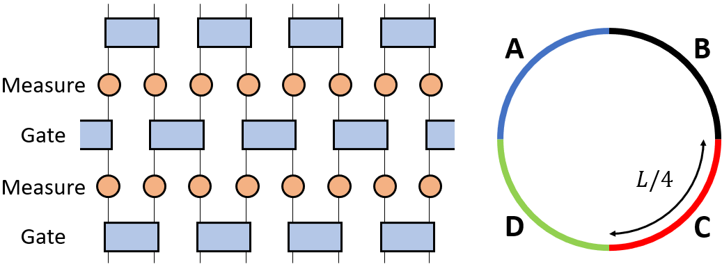
Figure 1: (left) Illustration of one step of our hybrid circuit model. Boxes correspond to 2-site random unitaries drawn from the Haar measure. Circles correspond to generalized $Z$ measurements, defined in the text. (right) The qubits are arranged on a ring with each quadrant labeled A-D.

The advantage of this Kraus operator formalism is that it can be applied to generalized measurements. For instance, a simple description of weak measurements is given by [2]

$$M_{0}^{NP} =\frac{1+\lambda Z}{\sqrt{2\left(1+\lambda^{2}\right)}}$$

$$M_{1}^{NP} =\frac{1-\lambda Z}{\sqrt{2\left(1+\lambda^{2}\right)}}$$ (1)

where the superscript “NP” indicates that the measurement is non-projective. Considering the action on a single qubit, we can again see this corresponds to a dephasing channel. As shown in the supplement [32] (which includes reference [33]),

$$\rho_{f}^{NP}=\left(\begin{array}[]{cc}\rho_{i,\uparrow\uparrow}&\left(\frac{1-\lambda^{2}}{1+\lambda^{2}}\right)\rho_{i,\uparrow\downarrow}\\ \left(\frac{1-\lambda^{2}}{1+\lambda^{2}}\right)\rho_{i,\downarrow\uparrow}&\rho_{i,\downarrow\downarrow}\end{array}\right).$$

Clearly the measurement-averaged dynamics match if $1-p=\frac{1-\lambda^{2}}{1+\lambda^{2}}$, suggesting that generalized measurement strength $\lambda$ corresponds to an effective measurement rate

$$p_{eff}^{NP}=\frac{2\lambda^{2}}{1+\lambda^{2}}$$ (2)

As we will see in the next section, both projective and non-projective measurements behave in a similar way, producing volume law phases at low $p_{eff}$ and area law at high $p_{eff}$. It might then be tempting to suggest that the phase transition is indeed identical for different models of the same measurement-averaged dynamics. However, we now show that this is not the case by considering a third generalized measurement protocol, which we refer to as unitary unfolding. In this case, with probability $q$, the qubit undergoes a unitary kick with operator $Z$. This is represented by Kraus operators

$$M_{0}^{U} =\sqrt{q}Z$$

$$M_{1}^{U} =\sqrt{1-q}\mathds{1}$$

Again, this corresponds to a pure dephasing channel, with identical measurement-averaged dynamics when

$$p_{eff}^{U}=2q.$$ (3)

While such unitary kicks do not collect information about the qubit, they are valid Kraus operators and therefore we refer to this situation as “unitary measurements” and use the superscript “$U$” .

Note that the limit of weak continuous measurement corresponds to Lindblad dynamics, meaning that the strong generalized measurements above can be generated by finite time evolution under appropriate unfoldings of the Lindblad equation. Therefore, we refer to these measurement-averaged dynamics as “Lindblad equivalent” and use the term Lindblad to refer to any such dynamics, even if the measurement amplitudes are not small.

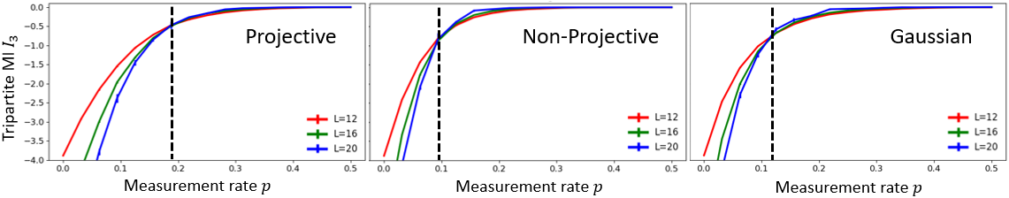
Figure 2: Comparison of tripartite mutual information (Eq. 4) between projective (P), non-projective (NP), and Gaussian (G, see Eq. 5) measurements over the same effective range of measurement rate $p$. Dashed lines show appromimate $p_{c}$ from finite size crossings, which clearly differs between measurement types.

Results – To confirm these predictions, we numerically examine the steady state entanglement under these measurement protocols using exact diagonalization. The conventional measure defining the phase transition is half-system von Neumann entanglement entropy,

$$S_{AB}=-\mathrm{Tr}\left[\rho_{AB}\log_{2}\rho_{AB}\right]$$

where $\rho_{AB}$ is the reduced density matrix of subsystem $AB$, which has length $L/2$ (see Figure 1). In principle, $S_{AB}$ is proportional to $L$ in the volume law phase and $O(1)$ in the area law phase. However, entanglement entropy has not been found to be a sensitive metric for the phase transition. Instead, we adopt the tripartite mutual information as used in [31]:

$$I_{3}=S_{A}+S_{B}+S_{C}+S_{D}-S_{AB}-S_{BC}-S_{AC}.$$ (4)

While $I_{3}$ is extensive (and negative) in the volume law phase, it vanishes in the thermodynamic limit within the area law phase, since boundary contribitions cancel. Therefore it provides much more useful finite size scaling for detecting the phase transition on small system size.

The entanglement entropy and tripartite mutual information are seen in Figure 2. The unitary unfolding is not shown explicitily, but for all $p$ it matches the $p=0$ limit of P and NP measurements.The first thing to note is that neither $S_{AB}$ nor $I_{3}$ matches for the three different unfoldings. This implies that the steady state ensembles are not microscopically equivalent, but not necessarily that the phases of matter differ. However, analyzing crossings of $I_{3}$ clarifies that the three unfoldings indeed give different phases and phase transitions. Most notably, the unitary unfolding has no phase transition, exhibiting a volume law phase for arbitrary $q=p/2$. By contrast, both the strong and weak measurements do exhibit phase transitions. Therefore, we see, as anticipated elsewhere, that different unfoldings of the measurement-averaged dynamics generally give different measurement-induced phase of matter. We note that the phase transitions are not guaranteed to be in the same universality class because, for instance, the unitary unfolding has no phase transition. Whether universality class of the phase transitions can differ away from the unitary limit is an open question for future work.

Having established that different unfoldings yield different measurement phase transitions, it is worth asking the question of which unfolding works best to minimize entanglement, allowing the area law phase to survive to the lowest $p_{c}$. To address this, we note that there is a general trend in the data: non-projective measurement consistently yields the smallest entanglement entropy, followed by random projective, and of course unitary measurement has the largest entanglement. This suggests that, among the measurements considered, non-projective would be the optimal unfolding for simulation by, e.g., matrix product states.

Before proceeding to argue that the non-projective measurement specified in Eq. 1 is optimal, we need simpler way to estimate the ability of a given measurement in terms of removing entanglement, under the assumption that a single measurement that removes entanglement will result in an overall lower entanglement within the many-body steady state. We propose a simple test, namely to determine how much entanglement is lost upon measuring one qubit in a maximally entangled state, such as the Bell state

$$|\psi_{\mathrm{Bell}}\rangle=\frac{|\uparrow\uparrow\rangle+|\downarrow\downarrow\rangle}{\sqrt{2}}.$$

The loss of entropy of the first qubit $\Delta S_{\mathrm{Bell}}=S_{f}-S_{i}$ is shown for various measurements in Figure 3. Clearly it aligns with the results for steady state entropy; a smaller steady state entropy density corresponds to larger $\left|\Delta S\right|$. To further test this theory, we consider a slightly more accurate model of weak measurement in which the histograms of measurement results are Gaussian distributed with a finite separation between $\uparrow$ and $\downarrow$ corresponding to the measurement strength $\alpha$ [30]

$$M^{G}(x)=2^{1/2}\pi^{1/4}\left[G\left(x-\alpha\right)|\uparrow\rangle\langle\uparrow|+G\left(x+\alpha\right)|\downarrow\rangle\langle\downarrow|\right]$$ (5)

where $G(x)$ is a normalized Gaussian of mean $0$ and variance $1$ and $x\in(-\infty,\infty)$ are the possible measurement outcomes. These Gaussian measurements further support our idea, as both the Bell state entropy loss $\Delta S_{\mathrm{Bell}}$ and the steady state entropy $S_{AB}$ are intermediate between non-projective and projective measurements.

Clearly non-projective measurements outperform random projective measurements in producing low-entanglement trajectories for the same Lindblad equation, i.e., are closer to the optimal unfolding for stochastic Schrödinger equation simulations. To argue that the measurements labeled “NP” are optimal, we consider the following generic family of generalized measurements:

$$M^{gen}(p,x)=\beta_{p}(x)\left[\mathds{1}+xZ\right],$$

a set of non-projective measurements weighted by the real function $\beta_{p}(x)=\beta_{p}(-x)$. As shown in the supplement [32], the function $\beta_{p}$ is constrained by a normalization condition, $\int_{-\infty}^{\infty}(1+x^{2})\beta_{p}(x)^{2}=1$, and our goal of matching the measurement-averaged dynamics, which sets $\int_{-\infty}^{\infty}x^{2}\beta_{p}(x)^{2}dx=p/2$. Note that all four of the measurement types considered so far fall within this family with appropriate choices of $\beta_{p}$. In order to better understand which $\beta_{p}$ will maximize $\left|\Delta S_{\mathrm{Bell}}\right|$, we start by noticing that, for each $x$, the measurement matches $M^{NP}(\lambda)$. As seen in Fig. 3 and shown analytically in the appendix, Bell state entropy loss is a convex function in the range $x\in[0,1]$, going from $\Delta S_{\mathrm{Bell}}=0$ at $x=0$ to $\Delta S_{\mathrm{Bell}}=1$ at $x=1$, which corresponds to a projective measurement. The precise opposite happens for $x>1$, as $\Delta S(x)=\Delta S(1/x)$. Therefore, the optimal entropy loss will be given by a $\delta$-function peaked at whatever value is necessary to match $p$, i.e., the non-projective (NP) measurement. While this argument is specific to our class of measurements and this particular system, we expect a similar line of logic to hold in attempting to determine optimal unfolding of more general Lindblad dynamics.

Discussion – We have shown explicitly that different unfoldings of the same measurement-averaged (Lindblad-type) dynamics give rise to different values of entanglement and the entanglement phase transition in the equivalent hybrid quantum circuit. We find that destruction of entanglement in a Bell pair is a useful proxy for many-body steady state entanglement for our class of hybrid circuits. We use this to show that a non-projective measurement of the form $\mathds{1}\pm\lambda Z$ is optimal for minimizing entanglement.

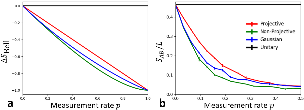
Figure 3: (a) Entanglement loss $\Delta S_{\mathrm{Bell}}$ after measurement of qubit 1 in a Bell pair and (b) steady state half-system entanglement entropy density $S_{AB}/L$. Many-body entropy $S_{AB}$ lines up precisely with $\Delta S_{\mathrm{Bell}}$ for all measurements considered, suggesting $\Delta S_{\mathrm{Bell}}$ as a useful proxy for optimal unfolding of the measurement-averaged dynamics.

The most immediate consequences of this work are for numerical simulations of open quantum systems via the stochastic Schrödinger equation, particularly for entanglement-sensitive methods such as matrix product states. Our work suggests to use an unfolding of the form $\mathds{1}+\lambda Z$ for dephasing channels, which are commonly found experimentally. We expect that a similar analysis can be applied for other Lindblad operators as well. Interestingly, our results imply that entanglement complexity of the stochastic Schrödinger equation is not equivalent to that of the Lindblad evolution, for example by simulating the density matrix directly as a matrix product operator. In particular, [35] showed that for unital quantum channels – like the ones we examine here – density matrices always flow to the area law phase and are thus efficiently representable. This implies that, for sufficiently slow Lindblad operators (small $p$), direct Lindblad evolution of the density matrix is more efficient than stochastic evolution of even a single pure state trajectory. The potential efficiency of density matrix evolution over trajectories was noted in [3]; this work adds to the picture by arguing that no trajectory unfolding can be as efficient as density matrix evolution.

In the longer term, this work may provide an interesting perspective on open quantum systems directly. In particular, the circuit models studied here are similar to models of noisy quantum devices, with environment playing the role of measurement, for which quantum error correction displays phase transitions at finite error rate [21]. It is clear from our results that no direct connection exists between measurement phase transitions and error correction in general, as error correction schemes must handle open quantum systems, e.g., Lindblad dynamics, whose measurement-induced phases behave differently for different unfoldings. However, there are clear similarities between these schemes which remain to be explored (cf. [36]). Further discussion of the general case in which syndrome measurement combined with environmental dissipation and error-correcting feedback can be interpreted through the lens of measurement phase transitions will be the subject of future work.

Acknowledgments – I am grateful for valuable discussions with Anushya Chandran, Sarang Gopalakrishnan, Tom Iadecola, Matteo Ippoliti, Vedika Khemani, Jed Pixley, Sagar Vijay, Justin Wilson, and Aidan Zahalo. I am particularly indebted to Aidan for sharing his code and Matteo for first suggesting the unitary measurement counterexample. This work was supported by the National Science Foundation through award number DMR-1945529 and the Welch Foundation through award number AT-2036-20200401. Part of this work was performed at the Aspen Center for Physics, which is supported by National Science Foundation grant PHY-1607611, and at the Kavli Institute for Theoretical Physics, which is supported by the National Science Foundation under Grant No. NSF PHY-1748958. Computational resources used include the Frontera cluster operated by the Texas Advanced Computing Center at the University of Texas at Austin and the Ganymede cluster operated by the University of Texas at Dallas’ Cyberinfrastructure & Research Services Department.

Supplementary Information

In this supplementary information, we derive measurement-averaged channels and Bell state entropy loss for each of the generalized measurements considered in the main text. We start by introducing a replica picture approach which also provides useful notation for doing measurement averages. We then derive the behavior of each generalized measurement using this machinery.

I Replica Picture

As shown in [20], the measurement phase transition can be obtained in the replica limit of a generalized Renyi entropy in which the vectorized density matrix is averaged over measurement outcomes in the replica picture. The advantage is that this reduces the trajectory-averaged entanglement entropy calculation, which is non-linear in density matrix, to a problem which is linear in replicated density matrix and, thus, more simple to calculate. As a warmup, consider the superoperator representation of the unreplicated state. For the case of a projective $Z$ measurement performed with probability $p$, the final density matrix can be written as

$$|\rho_{f}^{(1)}\rangle\rangle=\underbrace{\left[\left(1-p\right)\mathds{1}_{1}\mathds{1}_{\bar{1}}+p\Pi_{\uparrow 1}\Pi_{\uparrow\bar{1}}+p\Pi_{\downarrow 1}\Pi_{\downarrow\bar{1}}\right]}_{\mathcal{T}}|\rho_{i}^{(1)}\rangle\rangle$$

where $\Pi_{\uparrow}=|\uparrow\rangle\langle\uparrow|$ and the subscript $1$ ($\bar{1}$) indicates acting on the ket (bra). Rearranging, the transfer matrix $\mathcal{T}$ can be written

$$\mathcal{T}_{P}^{(1)} =\left(1-p\right)\mathds{1}_{1}\mathds{1}_{\bar{1}}+\frac{p}{4}\left(\mathds{1}_{1}+Z_{1}\right)\left(\mathds{1}_{\bar{1}}+Z_{\bar{1}}\right)+\frac{p}{4}\left(\mathds{1}_{1}-Z_{1}\right)\left(\mathds{1}_{\bar{1}}-Z_{\bar{1}}\right)$$

$$=\left(1-\frac{p}{2}\right)\mathds{1}_{1}\mathds{1}_{\bar{1}}+\frac{p}{2}Z_{1}Z_{\bar{1}}$$ (6)

Note that this is precisely the action of a single-qubit dephasing channel, which we will match for other generalized measurements in the following sections.

Now we do the same thing for the $n=2$ replica case:

$$\mathcal{T}_{P}^{(2)} =\left(1-p\right)^{2}\mathds{1}_{1}\mathds{1}_{\bar{1}}\mathds{1}_{2}\mathds{1}_{\bar{2}}+\frac{p^{2}}{16}\left(\mathds{1}_{1}+Z_{1}\right)\left(\mathds{1}_{\bar{1}}+Z_{\bar{1}}\right)\left(\mathds{1}_{2}+Z_{2}\right)\left(\mathds{1}_{\bar{2}}+Z_{\bar{2}}\right)$$

$$\;\;+\frac{p^{2}}{16}\left(\mathds{1}_{1}-Z_{1}\right)\left(\mathds{1}_{\bar{1}}-Z_{\bar{1}}\right)\left(\mathds{1}_{2}-Z_{2}\right)\left(\mathds{1}_{\bar{2}}-Z_{\bar{2}}\right)$$

$$=\left[1-2p+\frac{9p^{2}}{8}\right]\mathds{1}_{1}\mathds{1}_{\bar{1}}\mathds{1}_{2}\mathds{1}_{\bar{2}}+\frac{p^{2}}{8}\left(Z_{1}Z_{\bar{1}}+Z_{1}Z_{2}+Z_{1}Z_{\bar{2}}+Z_{\bar{1}}Z_{2}+Z_{\bar{1}}Z_{\bar{2}}+Z_{2}Z_{\bar{2}}\right)$$

$$\;\;+\frac{p^{2}}{8}Z_{1}Z_{\bar{1}}Z_{2}Z_{\bar{2}}$$

$$\mathcal{T}_{NP}^{(2)} =\frac{1}{4\left(1+\lambda^{2}\right)^{2}}\left(\mathds{1}_{1}+\lambda Z_{1}\right)\left(\mathds{1}_{\bar{1}}+\lambda Z_{\bar{1}}\right)\left(\mathds{1}_{2}+\lambda Z_{2}\right)\left(\mathds{1}_{\bar{2}}+\lambda Z_{\bar{2}}\right)+$$

$$\;\;\frac{1}{4\left(1+\lambda^{2}\right)^{2}}\left(\mathds{1}_{1}-\lambda Z_{1}\right)\left(\mathds{1}_{\bar{1}}-\lambda Z_{\bar{1}}\right)\left(\mathds{1}_{2}-\lambda Z_{2}\right)\left(\mathds{1}_{\bar{2}}-\lambda Z_{\bar{2}}\right)$$

$$=\frac{1}{2\left(1+\lambda^{2}\right)^{2}}\Bigg{[}\mathds{1}_{1}\mathds{1}_{\bar{1}}\mathds{1}_{2}\mathds{1}_{\bar{2}}+\lambda^{2}\left(Z_{1}Z_{\bar{1}}+Z_{1}Z_{2}+Z_{1}Z_{\bar{2}}+Z_{\bar{1}}Z_{2}+Z_{\bar{1}}Z_{\bar{2}}+Z_{2}Z_{\bar{2}}\right)$$

$$\;\;+\lambda^{4}Z_{1}Z_{\bar{1}}Z_{2}Z_{\bar{2}}\Bigg{]}$$

$$\mathcal{T}_{U}^{(2)} =\left(1-q\right)^{2}\mathds{1}_{1}\mathds{1}_{\bar{1}}\mathds{1}_{2}\mathds{1}_{\bar{2}}+q^{2}Z_{1}Z_{\bar{1}}Z_{2}Z_{\bar{2}}$$

$$\mathcal{T}_{G}^{(2)} =\pi\int dx\Bigg{\{}\left[G\left(x-\lambda\right)\left(\mathds{1}_{1}+Z_{1}\right)+G\left(x+\lambda\right)\left(\mathds{1}_{1}-Z_{1}\right)\right]\times$$

$$\;\;\;\;\;\;\left[G\left(x-\lambda\right)\left(\mathds{1}_{\bar{1}}+Z_{\bar{1}}\right)+G\left(x+\lambda\right)\left(\mathds{1}_{\bar{1}}-Z_{\bar{1}}\right)\right]\times$$

$$\;\;\;\;\;\;\left[G\left(x-\lambda\right)\left(\mathds{1}_{2}+Z_{2}\right)+G\left(x+\lambda\right)\left(\mathds{1}_{2}-Z_{2}\right)\right]\times$$

$$\;\;\;\;\;\;\left[G\left(x-\lambda\right)\left(\mathds{1}_{\bar{2}}+Z_{\bar{2}}\right)+G\left(x+\lambda\right)\left(\mathds{1}_{\bar{2}}-Z_{\bar{2}}\right)\right]\Bigg{\}}$$

$$=\pi\int dx\left[G\left(x-\lambda\right)\right]^{4}\mathds{1}_{1}\mathds{1}_{\bar{1}}\mathds{1}_{2}\mathds{1}_{\bar{2}}+$$

$$\;\;\pi\int dx\left[G\left(x-\lambda\right)\right]^{2}\left[G\left(x+\lambda\right)\right]^{2}\left(Z_{1}Z_{\bar{1}}+Z_{1}Z_{2}+Z_{1}Z_{\bar{2}}+Z_{\bar{1}}Z_{2}+Z_{\bar{1}}Z_{\bar{2}}+Z_{2}Z_{\bar{2}}\right)+$$

$$\;\;\pi\int dx\left[G\left(x+\lambda\right)\right]^{4}Z_{1}Z_{\bar{1}}Z_{2}Z_{\bar{2}}$$

$$\int dx\left[G\left(x-\lambda\right)\right]^{4} =\int dx\frac{G(2\left(x-\lambda\right))}{2\pi}=\frac{1}{4\pi}$$

$$\int dx\left[G\left(x-\lambda\right)\right]^{2}\left[G\left(x+\lambda\right)\right]^{2} =\frac{1}{4\pi^{2}}\int dx\exp\left[-\frac{\left(x-\lambda\right)^{2}}{2}-\frac{\left(x+\lambda\right)^{2}}{2}\right]$$

$$=\frac{1}{4\pi^{2}}\int dx\exp\left[-x^{2}-\lambda^{2}\right]=\frac{e^{-\lambda^{2}}}{4\pi^{3/2}}$$

$$\mathcal{T}_{G}^{(2)} =\frac{1}{4}\left[\mathds{1}_{1}\mathds{1}_{\bar{1}}\mathds{1}_{2}\mathds{1}_{\bar{2}}+\frac{e^{-\lambda^{2}}}{\sqrt{\pi}}\left(Z_{1}Z_{\bar{1}}+Z_{1}Z_{2}+Z_{1}Z_{\bar{2}}+Z_{\bar{1}}Z_{2}+Z_{\bar{1}}Z_{\bar{2}}+Z_{2}Z_{\bar{2}}\right)+Z_{1}Z_{\bar{1}}Z_{2}Z_{\bar{2}}\right]$$

An interesting fact, which will hold at higher $n$ as well, is that the unitary case does not contain the pairwise $Z_{i}Z_{j}$ terms, while both the projective and non-projective case do. However, coefficients for projective versus non-projective are different, which will result in differences between their entanglement. For instance, at leading order in $p,\lambda\ll 1$, the projective case would have both the pairwise and four “qubit” ($Z_{1}Z_{\bar{1}}Z_{2}Z_{\bar{2}}$) terms, whereas the non-projective case would just include the pairwise term. Thus, even in this Lindblad limit, the projective and non-projective cases are different for $n=2$ replicas.

In order to understand the role of such measurements in disentangling the system within this replica picture, let’s consider the general case

$$\mathcal{T}^{(2)}\sim\mathds{1}_{1}\mathds{1}_{\bar{1}}\mathds{1}_{2}\mathds{1}_{\bar{2}}+\alpha\left(Z_{1}Z_{\bar{1}}+Z_{1}Z_{2}+Z_{1}Z_{\bar{2}}+Z_{\bar{1}}Z_{2}+Z_{\bar{1}}Z_{\bar{2}}+Z_{2}Z_{\bar{2}}\right)+\beta Z_{1}Z_{\bar{1}}Z_{2}Z_{\bar{2}}$$

acting on a Bell state $|\psi\rangle=\left(|\uparrow\uparrow\rangle+|\downarrow\downarrow\rangle\right)/\sqrt{2}$. Let’s start by introducing notation for our replicated states:

$$|\rho_{i}^{(2)}\rangle\rangle =\frac{1}{4}\left(|\uparrow\uparrow\rangle+|\downarrow\downarrow\rangle\right)\otimes\left(\langle\uparrow\uparrow|+\langle\downarrow\downarrow|\right)\otimes\left(|\uparrow\uparrow\rangle+|\downarrow\downarrow\rangle\right)\otimes\left(\langle\uparrow\uparrow|+\langle\downarrow\downarrow|\right)$$

$$\equiv\frac{1}{4}\left(|\uparrow\uparrow\uparrow\uparrow\uparrow\uparrow\uparrow\uparrow\rangle\rangle+|\uparrow\uparrow\downarrow\downarrow\uparrow\uparrow\uparrow\uparrow\rangle\rangle+|\uparrow\uparrow\uparrow\uparrow\downarrow\downarrow\uparrow\uparrow\rangle\rangle+\cdots+|\downarrow\downarrow\downarrow\downarrow\downarrow\downarrow\downarrow\downarrow\rangle\rangle\right)$$

where we have defined the replicated density matrix supervector via eigenstates of the basis

$$|Z_{1,1}Z_{2,1}Z_{1,\bar{1}}Z_{2,\bar{1}}Z_{1,2}Z_{2,2}Z_{1,\bar{2}}Z_{2,\bar{2}}\rangle\rangle$$

where $Z_{i,j}$ corresponds to replica $j$ of spin at site $i$. The initial density matrix contains 16 terms in which spin 1 and 2 are aligned independently for each replica and bra/ket. For comparison, the identity state corresponds to $\mathds{1}$ for each spin and replica independently. In our language, this corresponds to an equal superposition over spin states in which the bra and the ket ($j$ and $\bar{j}$) match,

$$|I^{(2)}\rangle\rangle=|\uparrow\uparrow\uparrow\uparrow\uparrow\uparrow\uparrow\uparrow\rangle\rangle+|\downarrow\uparrow\downarrow\uparrow\uparrow\uparrow\uparrow\uparrow\rangle\rangle+|\uparrow\downarrow\uparrow\downarrow\uparrow\uparrow\uparrow\uparrow\rangle\rangle+\cdots+|\downarrow\downarrow\downarrow\downarrow\downarrow\downarrow\downarrow\downarrow\rangle\rangle$$

up to an overall prefactor that we define as $1$. Consider the pairwise and quartic “interactions”:

$$\mathcal{T}_{pair}^{(2)}|\rho_{i}^{(2)}\rangle\rangle =\frac{1}{4}\Bigg{[}6|\uparrow\uparrow\uparrow\uparrow\uparrow\uparrow\uparrow\uparrow\rangle\rangle+0|\uparrow\uparrow\uparrow\uparrow\uparrow\uparrow\downarrow\downarrow\rangle\rangle+0|\uparrow\uparrow\uparrow\uparrow\downarrow\downarrow\uparrow\uparrow\rangle\rangle-2|\uparrow\uparrow\uparrow\uparrow\downarrow\downarrow\downarrow\downarrow\rangle\rangle+$$

$$\;\;\;\;\;\;0|\uparrow\uparrow\downarrow\downarrow\uparrow\uparrow\uparrow\uparrow\rangle\rangle-2|\uparrow\uparrow\downarrow\downarrow\uparrow\uparrow\downarrow\downarrow\rangle\rangle-2|\uparrow\uparrow\downarrow\downarrow\downarrow\downarrow\uparrow\uparrow\rangle\rangle+0|\uparrow\uparrow\downarrow\downarrow\downarrow\downarrow\downarrow\downarrow\rangle\rangle+$$

$$\;\;\;\;\;\;0|\downarrow\downarrow\uparrow\uparrow\uparrow\uparrow\uparrow\uparrow\rangle\rangle-2|\downarrow\downarrow\uparrow\uparrow\uparrow\uparrow\downarrow\downarrow\rangle\rangle-2|\downarrow\downarrow\uparrow\uparrow\downarrow\downarrow\uparrow\uparrow\rangle\rangle+0|\downarrow\downarrow\uparrow\uparrow\downarrow\downarrow\downarrow\downarrow\rangle\rangle-$$

$$\;\;\;\;\;\;2|\downarrow\downarrow\downarrow\downarrow\uparrow\uparrow\uparrow\uparrow\rangle\rangle+0|\downarrow\downarrow\downarrow\downarrow\uparrow\uparrow\downarrow\downarrow\rangle\rangle+0|\downarrow\downarrow\downarrow\downarrow\downarrow\downarrow\uparrow\uparrow\rangle\rangle+6|\downarrow\downarrow\downarrow\downarrow\downarrow\downarrow\downarrow\downarrow\rangle\rangle\Bigg{]}$$

$$\mathcal{T}_{quart}^{(2)}|\rho_{i}^{(2)}\rangle\rangle =\frac{1}{4}\Bigg{[}|\uparrow\uparrow\uparrow\uparrow\uparrow\uparrow\uparrow\uparrow\rangle\rangle-|\uparrow\uparrow\uparrow\uparrow\uparrow\uparrow\downarrow\downarrow\rangle\rangle-|\uparrow\uparrow\uparrow\uparrow\downarrow\downarrow\uparrow\uparrow\rangle\rangle+|\uparrow\uparrow\uparrow\uparrow\downarrow\downarrow\downarrow\downarrow\rangle\rangle-$$

$$\;\;\;\;\;\;|\uparrow\uparrow\downarrow\downarrow\uparrow\uparrow\uparrow\uparrow\rangle\rangle+|\uparrow\uparrow\downarrow\downarrow\uparrow\uparrow\downarrow\downarrow\rangle\rangle+|\uparrow\uparrow\downarrow\downarrow\downarrow\downarrow\uparrow\uparrow\rangle\rangle-|\uparrow\uparrow\downarrow\downarrow\downarrow\downarrow\downarrow\downarrow\rangle\rangle-$$

$$\;\;\;\;\;\;|\downarrow\downarrow\uparrow\uparrow\uparrow\uparrow\uparrow\uparrow\rangle\rangle+|\downarrow\downarrow\uparrow\uparrow\uparrow\uparrow\downarrow\downarrow\rangle\rangle+|\downarrow\downarrow\uparrow\uparrow\downarrow\downarrow\uparrow\uparrow\rangle\rangle-|\downarrow\downarrow\uparrow\uparrow\downarrow\downarrow\downarrow\downarrow\rangle\rangle+$$

$$\;\;\;\;\;\;|\downarrow\downarrow\downarrow\downarrow\uparrow\uparrow\uparrow\uparrow\rangle\rangle-|\downarrow\downarrow\downarrow\downarrow\uparrow\uparrow\downarrow\downarrow\rangle\rangle-|\downarrow\downarrow\downarrow\downarrow\downarrow\downarrow\uparrow\uparrow\rangle\rangle+|\downarrow\downarrow\downarrow\downarrow\downarrow\downarrow\downarrow\downarrow\rangle\rangle\Bigg{]}$$

Putting these terms together,

$$|\rho_{f}^{(2)}\rangle\rangle =\frac{1}{4}\Bigg{[}\left(1+6\alpha+\beta\right)|\uparrow\uparrow\uparrow\uparrow\uparrow\uparrow\uparrow\uparrow\rangle\rangle+\left(1-\beta\right)|\uparrow\uparrow\uparrow\uparrow\uparrow\uparrow\downarrow\downarrow\rangle\rangle+\left(1-\beta\right)|\uparrow\uparrow\uparrow\uparrow\downarrow\downarrow\uparrow\uparrow\rangle\rangle+\left(1-2\alpha+\beta\right)|\uparrow\uparrow\uparrow\uparrow\downarrow\downarrow\downarrow\downarrow\rangle\rangle+$$

$$\;\;\;\;\;\;\left(1-\beta\right)|\uparrow\uparrow\downarrow\downarrow\uparrow\uparrow\uparrow\uparrow\rangle\rangle+\left(1-2\alpha+\beta\right)|\uparrow\uparrow\downarrow\downarrow\uparrow\uparrow\downarrow\downarrow\rangle\rangle+\left(1-2\alpha+\beta\right)|\uparrow\uparrow\downarrow\downarrow\downarrow\downarrow\uparrow\uparrow\rangle\rangle+\left(1-\beta\right)|\uparrow\uparrow\downarrow\downarrow\downarrow\downarrow\downarrow\downarrow\rangle\rangle+$$

$$\;\;\;\;\;\;\left(1-\beta\right)|\downarrow\downarrow\uparrow\uparrow\uparrow\uparrow\uparrow\uparrow\rangle\rangle+\left(1-2\alpha+\beta\right)|\downarrow\downarrow\uparrow\uparrow\uparrow\uparrow\downarrow\downarrow\rangle\rangle+\left(1-2\alpha+\beta\right)|\downarrow\downarrow\uparrow\uparrow\downarrow\downarrow\uparrow\uparrow\rangle\rangle+\left(1-\beta\right)|\downarrow\downarrow\uparrow\uparrow\downarrow\downarrow\downarrow\downarrow\rangle\rangle+$$

$$\;\;\;\;\;\;\left(1+\beta\right)|\downarrow\downarrow\downarrow\downarrow\uparrow\uparrow\uparrow\uparrow\rangle\rangle+\left(1-\beta\right)|\downarrow\downarrow\downarrow\downarrow\uparrow\uparrow\downarrow\downarrow\rangle\rangle+\left(1-\beta\right)|\downarrow\downarrow\downarrow\downarrow\downarrow\downarrow\uparrow\uparrow\rangle\rangle+\left(1+6\alpha+\beta\right)|\downarrow\downarrow\downarrow\downarrow\downarrow\downarrow\downarrow\downarrow\rangle\rangle\Bigg{]}$$

The entanglement is calculated as the replica limit of

$$S_{A}^{(n)} =\frac{1}{1-n}\log_{2}\left[\frac{\langle\langle I|C_{A}^{(n)}|\rho^{(n)}\rangle\rangle}{\langle\langle I|\rho^{(n)}\rangle\rangle}\right]$$

where $C_{A}^{(n)}$ permutes replicas in subsystem $A$. Consider our case for $A$ given by site 1.

$$C_{A}^{(2)}|\rho_{i}^{(2)}\rangle\rangle =\frac{1}{4}\Bigg{[}|\uparrow\uparrow\uparrow\uparrow\uparrow\uparrow\uparrow\uparrow\rangle\rangle+|\uparrow\uparrow\uparrow\uparrow\uparrow\uparrow\downarrow\downarrow\rangle\rangle+|\downarrow\uparrow\uparrow\uparrow\uparrow\downarrow\uparrow\uparrow\rangle\rangle+|\downarrow\uparrow\uparrow\uparrow\uparrow\downarrow\downarrow\downarrow\rangle\rangle+$$

$$\;\;\;\;\;\;|\uparrow\uparrow\downarrow\downarrow\uparrow\uparrow\uparrow\uparrow\rangle\rangle+|\uparrow\uparrow\downarrow\downarrow\uparrow\uparrow\downarrow\downarrow\rangle\rangle+|\downarrow\uparrow\downarrow\downarrow\uparrow\downarrow\uparrow\uparrow\rangle\rangle+|\downarrow\uparrow\downarrow\downarrow\uparrow\downarrow\downarrow\downarrow\rangle\rangle+$$

$$\;\;\;\;\;\;|\uparrow\downarrow\uparrow\uparrow\downarrow\uparrow\uparrow\uparrow\rangle\rangle+|\uparrow\downarrow\uparrow\uparrow\downarrow\uparrow\downarrow\downarrow\rangle\rangle+|\downarrow\downarrow\uparrow\uparrow\downarrow\downarrow\uparrow\uparrow\rangle\rangle+|\downarrow\downarrow\uparrow\uparrow\downarrow\downarrow\downarrow\downarrow\rangle\rangle+$$

$$\;\;\;\;\;\;|\uparrow\downarrow\downarrow\downarrow\downarrow\uparrow\uparrow\uparrow\rangle\rangle+|\uparrow\downarrow\downarrow\downarrow\downarrow\uparrow\downarrow\downarrow\rangle\rangle+|\downarrow\downarrow\downarrow\downarrow\downarrow\downarrow\uparrow\uparrow\rangle\rangle+|\downarrow\downarrow\downarrow\downarrow\downarrow\downarrow\downarrow\downarrow\rangle\rangle\Bigg{]}$$

$$C_{A}^{(2)}|\rho_{f}^{(2)}\rangle\rangle =\frac{1}{4}\Bigg{[}\left(1+6\alpha+\beta\right)|\uparrow\uparrow\uparrow\uparrow\uparrow\uparrow\uparrow\uparrow\rangle\rangle+\left(1-\beta\right)|\uparrow\uparrow\uparrow\uparrow\uparrow\uparrow\downarrow\downarrow\rangle\rangle+\left(1-\beta\right)|\downarrow\uparrow\uparrow\uparrow\uparrow\downarrow\uparrow\uparrow\rangle\rangle+\left(1+\beta\right)|\downarrow\uparrow\uparrow\uparrow\uparrow\downarrow\downarrow\downarrow\rangle\rangle+$$

$$\;\;\;\;\;\;\left(1-\beta\right)|\uparrow\uparrow\downarrow\downarrow\uparrow\uparrow\uparrow\uparrow\rangle\rangle+\left(1+\beta\right)|\uparrow\uparrow\downarrow\downarrow\uparrow\uparrow\downarrow\downarrow\rangle\rangle+\left(1+\beta\right)|\downarrow\uparrow\downarrow\downarrow\uparrow\downarrow\uparrow\uparrow\rangle\rangle+\left(1-\beta\right)|\downarrow\uparrow\downarrow\downarrow\uparrow\downarrow\downarrow\downarrow\rangle\rangle+$$

$$\;\;\;\;\;\;\left(1-\beta\right)|\uparrow\downarrow\uparrow\uparrow\downarrow\uparrow\uparrow\uparrow\rangle\rangle+\left(1+\beta\right)|\uparrow\downarrow\uparrow\uparrow\downarrow\uparrow\downarrow\downarrow\rangle\rangle+\left(1+\beta\right)|\downarrow\downarrow\uparrow\uparrow\downarrow\downarrow\uparrow\uparrow\rangle\rangle+\left(1-\beta\right)|\downarrow\downarrow\uparrow\uparrow\downarrow\downarrow\downarrow\downarrow\rangle\rangle+$$

$$\;\;\;\;\;\;\left(1-2\alpha+\beta\right)|\uparrow\downarrow\downarrow\downarrow\downarrow\uparrow\uparrow\uparrow\rangle\rangle+\left(1-\beta\right)|\uparrow\downarrow\downarrow\downarrow\downarrow\uparrow\downarrow\downarrow\rangle\rangle+\left(1-\beta\right)|\downarrow\downarrow\downarrow\downarrow\downarrow\downarrow\uparrow\uparrow\rangle\rangle+\left(1+6\alpha+\beta\right)|\downarrow\downarrow\downarrow\downarrow\downarrow\downarrow\downarrow\downarrow\rangle\rangle\Bigg{]}$$

$$2^{-S_{A,i}^{(2)}} =\frac{\langle\langle I|C_{A}^{(2)}|\rho_{i}^{(2)}\rangle\rangle}{\langle\langle I|\rho_{i}^{(2)}\rangle\rangle}=\frac{1}{2}$$

$$2^{-S_{A,f}^{(2)}} =\frac{2\left(1+6\alpha+\beta\right)}{2\left(1+6\alpha+\beta\right)+2\left(1-2\alpha+\beta\right)}=\frac{1+6\alpha+\beta}{2+4\alpha+2\beta}$$

For the fully projective case, $\alpha=\beta=1$, this gives the expected result $e^{-S_{A}^{(2)}}=1$, i.e., zero entanglement. In general, this is a useful metric to determine how much entanglement is lost, on average, when a generalized measurement is performed. One advantage is that it is more straightforward to calculate than von Neumann entropy. However, since von Neumann entropy is more commonly used to obtain the measurement phase transition, we solve it below and focus on it in the main text.

II Random Projective Measurement (P)

We now proceed to calculate details for the various generalized measurements calculated in the main text. Let’s start with random projective measurement. This can be made into a generalized measurement performed on each site by introducing a third measurement operator that does nothing. Specifically, the complete set of measurement operators is

$$M_{0} =\sqrt{p}|0\rangle\langle 0|\equiv\sqrt{p}\Pi_{0}$$

$$M_{1} =\sqrt{p}|1\rangle\langle 1|\equiv\sqrt{p}\Pi_{1}$$

$$M_{2} =\sqrt{1-p}\mathds{1}$$

These (Hermitian) measurement operators clearly satisfy the completeness relation $\sum_{j}M_{j}^{\dagger}M_{j}=\mathds{1}$. Meanwhile, their action on the density matrix is that of dephasing:

$$\rho_{f} =\sum_{j}M_{j}\rho_{i}M_{j}^{\dagger}$$

$$=p\rho_{i,00}|0\rangle\langle 0|+p\rho_{i,11}|1\rangle\langle 1|+\left(1-p\right)\rho_{i}$$

$$=\left(\begin{array}[]{cc}\rho_{i,00}&\left(1-p\right)\rho_{i,01}\\ \left(1-p\right)\rho_{i,10}&\rho_{i,11}\end{array}\right)$$

This is precisely the effect of $T_{2}$ dephasing applied for time $t$ such that $1-p=e^{-t/T_{2}}$. Note that this is a circuit version of the Lindblad equation. It could be replaced by actual time-dependent Lindblad dynamics by simply replacing the measurement step by Lindblad dynamics for finite time with single Lindblad operator $Z$.

It is also worth noting that the same Lindblad-type action can be obtained directly through the superoperator formalism. As seen in Eq. 6,

$$\mathcal{T}_{P}^{(1)}=\left(1-p\right)\mathds{1}_{1}\mathds{1}_{\bar{1}}+\frac{p}{4}\left(\mathds{1}_{1}+Z_{1}\right)\left(\mathds{1}_{\bar{1}}+Z_{\bar{1}}\right)+\frac{p}{4}\left(\mathds{1}_{1}-Z_{1}\right)\left(\mathds{1}_{\bar{1}}-Z_{\bar{1}}\right)=\left(1-\frac{p}{2}\right)\mathds{1}_{1}\mathds{1}_{\bar{1}}+\frac{p}{2}Z_{1}Z_{\bar{1}}.$$

This is the transfer matrix, i.e., measurement-averaged quantum channel, that we will match throughout this supplement for various measurement types.

The final entropy of the Bell state is readily calculated by noting that it is $0$ if a measurement is done and remains $1$ if no measurement is done. Hence,

$$S_{f}^{P}=\left(1-p\right)\left(1\right)+\frac{p}{2}\left(0\right)+\frac{p}{2}\left(0\right)=1-p.$$

III Definite Non-Projective Measurement (NP)

Next, consider the non-projective (NP) measurements:

$$M_{\pm}=\frac{1\pm\lambda Z}{\sqrt{2\left(1+\lambda^{2}\right)}}$$

For these measurements, we have

$$\mathcal{T}_{NP}^{(1)} =\frac{1}{2\left(1+\lambda^{2}\right)}\left(\mathds{1}_{1}+\lambda Z_{1}\right)\left(\mathds{1}_{\bar{1}}+\lambda Z_{\bar{1}}\right)+\frac{1}{2\left(1+\lambda^{2}\right)}\left(\mathds{1}_{1}-\lambda Z_{1}\right)\left(\mathds{1}_{\bar{1}}-\lambda Z_{\bar{1}}\right)$$

$$=\frac{1}{\left(1+\lambda^{2}\right)}\mathds{1}_{1}\mathds{1}_{\bar{1}}+\frac{\lambda^{2}}{\left(1+\lambda^{2}\right)}Z_{1}Z_{\bar{1}}$$ (7)

Note that Eq. 6 and 7 match if $p=2\lambda^{2}/\left(1+\lambda^{2}\right)$, as expected.

Next let’s calculate $\Delta S_{\mathrm{Bell}}$ for NP measurements. After measurement result $+$ on qubit $1$,

$$|\psi_{+}\rangle =M_{+1}|\psi_{\mathrm{Bell}}\rangle$$

$$=\frac{\left(1+\lambda\right)|\uparrow\uparrow\rangle+\left(1-\lambda\right)|\downarrow\downarrow\rangle}{2\left(1+\lambda^{2}\right)}$$

$$\rho_{f1}(x) =\frac{1}{2\left(1+\lambda^{2}\right)}\left(\begin{array}[]{cc}\left(1+\lambda\right)^{2}&0\\ 0&\left(1-\lambda\right)^{2}\end{array}\right)$$

$$S_{f}(\lambda) =\frac{\left(1+\lambda\right)^{2}}{2\left(1+\lambda^{2}\right)}\log_{2}\left[\frac{2\left(1+\lambda^{2}\right)}{\left(1+\lambda\right)^{2}}\right]+\frac{\left(1-\lambda\right)^{2}}{2\left(1-\lambda^{2}\right)}\log_{2}\left[\frac{2\left(1-\lambda^{2}\right)}{\left(1-\lambda\right)^{2}}\right]$$

The same reduced density matrix results for measurement result $-$, except with the role of $\uparrow$ and $\downarrow$ reversed. Therefore, entanglement entropy does not depend on measurement outcome. Note that

$$\rho_{f1}(\lambda^{-1}) =\frac{1}{2\left(1+\lambda^{-2}\right)}\left(\begin{array}[]{cc}\left(1+\lambda^{-1}\right)^{2}&0\\ 0&\left(1-\lambda^{-1}\right)^{2}\end{array}\right)$$

$$=\frac{1}{2\left(1+\lambda^{-2}\right)}\left(\begin{array}[]{cc}\lambda^{-2}\left(\lambda+1\right)^{2}&0\\ 0&\lambda^{-2}\left(\lambda-1\right)^{2}\end{array}\right)$$

$$=\frac{1}{2\left(1+\lambda^{2}\right)}\left(\begin{array}[]{cc}\left(1+\lambda\right)^{2}&0\\ 0&\left(1-\lambda\right)^{2}\end{array}\right)=\rho_{f1}(\lambda)$$

so $S_{f}(\lambda)=S_{f}(1/\lambda)$.

IV Unitary Measurement (U)

Consider the unitary measurement given by Kraus operators

$$M_{0} =\sqrt{p_{U}}Z$$

$$M_{1} =\sqrt{1-p_{U}}\mathds{1}$$

Then

$$\mathcal{T}_{U}^{(1)}=\left(1-q\right)\mathds{1}_{1}\mathds{1}_{\bar{1}}+qZ_{1}Z_{\bar{1}}$$

with matching for $q=p/2$. It is clear without calculation that single site unitaries do not affect entanglement, so $\Delta S_{\mathrm{Bell}}=0$.

V Gaussian Weak Measurement (G)

A Gaussian model of weak measurement is more consistent with experimental realizations (cf. [33]) and has been considered in other papers on the measurement phase transition [30]. The Krauss operators are

$$M^{G}(x)=2^{1/2}\pi^{1/4}\left[G\left(x-\alpha\right)\Pi_{\uparrow}+G\left(x+\alpha\right)\Pi_{\downarrow}\right]$$

where $G(z)\propto\exp\left(-z^{2}/2\right)$ is a normalized Gaussian of mean zero and standard deviation 1. Noting that

$$G^{2}(z) =\frac{1}{2\pi}e^{-z^{2}}$$

$$=\frac{1}{\left(\sqrt{2\pi}\right)^{2}}e^{-\left(z\sqrt{2}\right)^{2}/2}$$

$$=\frac{G(z\sqrt{2})}{\sqrt{2\pi}}$$

and that the measurement operators are again Hermitian, they satisfy the appropriate completeness relation:

$$\int_{-\infty}^{\infty}dx\left[2^{1/2}\pi^{1/4}G\left(x-\alpha\right)\right]^{2} =\frac{2\sqrt{\pi}}{\sqrt{2\pi}}\int_{-\infty}^{\infty}dxG\left(\underbrace{\left(x-\alpha\right)\sqrt{2}}_{z^{\prime}}\right)$$

$$=\sqrt{2}\left(\frac{1}{\sqrt{2}}\right)\int_{-\infty}^{\infty}dz^{\prime}G\left(z^{\prime}\right)$$

$$=1$$

$$\int_{-\infty}^{\infty}dxM^{G}(x)^{\dagger}M^{G}(x) =\mathds{1}$$

The transfer matrix is

$$\mathcal{T}_{G}^{(1)} =\int_{-\infty}^{\infty}dxM_{1}^{G}(x)M_{\bar{1}}^{G}(x)$$

$$=2\sqrt{\pi}\int_{-\infty}^{\infty}dx\left[G\left(x-\alpha\right)\Pi_{\uparrow 1}+G\left(x+\alpha\right)\Pi_{\downarrow 1}\right]\left[G\left(x-\alpha\right)\Pi_{\uparrow\bar{1}}+G\left(x+\alpha\right)\Pi_{\downarrow\bar{1}}\right]$$

$$2\sqrt{\pi}\int_{-\infty}^{\infty}dxG\left(x-\alpha\right)G\left(x+\alpha\right) =2\pi^{1/2}\left(\frac{1}{2\pi}\right)\int_{-\infty}^{\infty}dx\exp\left[-\frac{1}{2}\left(x-\alpha\right)^{2}-\frac{1}{2}\left(x6\alpha\right)^{2}\right]$$

$$=\frac{1}{\sqrt{\pi}}\int_{-\infty}^{\infty}dx\exp\left[-x^{2}-\alpha^{2}\right]$$

$$=\exp\left[-\alpha^{2}\right]$$

$$\mathcal{T}_{G}^{(1)} =\Pi_{\uparrow 1}\Pi_{\uparrow\bar{1}}+e^{-\alpha^{2}}\Pi_{\uparrow 1}\Pi_{\downarrow\bar{1}}+e^{-\alpha^{2}}\Pi_{\downarrow 1}\Pi_{\uparrow\bar{1}}+\Pi_{\downarrow 1}\Pi_{\downarrow\bar{1}}$$

$$=\frac{1}{4}\Bigg{[}\left(\mathds{1}_{1}+Z_{1}\right)\left(\mathds{1}_{\bar{1}}+Z_{\bar{1}}\right)+e^{-\alpha^{2}}\left(\mathds{1}_{1}+Z_{1}\right)\left(\mathds{1}_{\bar{1}}-Z_{\bar{1}}\right)+$$

$$\;\;\;\;\;\;e^{-\alpha^{2}}\left(\mathds{1}_{1}-Z_{1}\right)\left(\mathds{1}_{\bar{1}}+Z_{\bar{1}}\right)+\left(\mathds{1}_{1}-Z_{1}\right)\left(\mathds{1}_{\bar{1}}-Z_{\bar{1}}\right)\Bigg{]}$$

$$=\frac{1}{2}\left[\left(1+e^{-\alpha^{2}}\right)\mathds{1}_{1}\mathds{1}_{\bar{1}}+\left(1-e^{-\alpha^{2}}\right)Z_{1}Z_{\bar{1}}\right]$$

$$\implies p =1-e^{-\alpha^{2}}.$$

Calculating the final entropy of the Bell state is possible. Note that, given the continuum of measurement outcomes $x$, the results for each state must be weighted by the probability of obtaining that $x$ value. Therefore,

$$|\psi^{G}\left(x\right)\rangle =\frac{e^{-\left(x-\alpha\right)^{2}/2}|\uparrow\uparrow\rangle+e^{-\left(x+\alpha\right)^{2}/2}|\downarrow\downarrow\rangle}{\sqrt{e^{-\left(x-\alpha\right)^{2}}+e^{-\left(x+\alpha\right)^{2}}}}$$

$$S^{G}(x) =\frac{e^{-\left(x-\alpha\right)^{2}}}{e^{-\left(x-\alpha\right)^{2}}+e^{-\left(x+\alpha\right)^{2}}}\log_{2}\left[\frac{e^{-\left(x-\alpha\right)^{2}}}{e^{-\left(x-\alpha\right)^{2}}+e^{-\left(x+\alpha\right)^{2}}}\right]+\frac{e^{-\left(x+\alpha\right)^{2}}}{e^{-\left(x-\alpha\right)^{2}}+e^{-\left(x+\alpha\right)^{2}}}\log_{2}\left[\frac{e^{-\left(x+\alpha\right)^{2}}}{e^{-\left(x-\alpha\right)^{2}}+e^{-\left(x+\alpha\right)^{2}}}\right]$$

$$p(x) =\langle\psi_{i}|M^{2}(x)|\psi_{i}\rangle=2\sqrt{\pi}\left[G\left(x-\alpha\right)^{2}\left(\frac{1}{2}\right)+G\left(x+\alpha\right)^{2}\left(\frac{1}{2}\right)\right]$$

$$=\frac{1}{2\sqrt{\pi}}\left[e^{-\left(x-\alpha\right)^{2}}+e^{-\left(x+\alpha\right)^{2}}\right]$$

$$S_{f}^{G} =\int_{-\infty}^{\infty}dxp(x)S^{G}(x)=\frac{1}{2\sqrt{\pi}}\int_{-\infty}^{\infty}dx\left(e^{-\left(x-\alpha\right)^{2}}\log_{2}\left[\frac{e^{-\left(x-\alpha\right)^{2}}}{e^{-\left(x-\alpha\right)^{2}}+e^{-\left(x+\alpha\right)^{2}}}\right]+e^{-\left(x+\alpha\right)^{2}}\log_{2}\left[\frac{e^{-\left(x+\alpha\right)^{2}}}{e^{-\left(x-\alpha\right)^{2}}+e^{-\left(x+\alpha\right)^{2}}}\right]\right)$$

The final integral can be calculated numerically, obtaining the results in Figure 3 of the main text.

VI Universal Generalized Measurements (gen)

Finally, we consider a family of generalized measurements that encompasses all previous ones,

$$M^{gen}(p,x)=\beta_{p}(x)\left[\mathds{1}+xZ\right],$$

with the restriction $\beta_{p}(-x)=\beta_{p}(x)$ on the real-valued function $\beta_{p}$. Normalization of the Kraus operators gives

$$\mathds{1} =\int_{-\infty}^{\infty}\left[M^{G}(p,x)\right]^{2}dx$$

$$=\mathds{1}\int_{-\infty}^{\infty}(1+x^{2})\beta_{p}(x)^{2}dx$$

$$\implies\int_{-\infty}^{\infty}(1+x^{2})\beta_{p}(x)^{2} =1$$

To match the Lindblad operator with measurement strength $p$, we need

$$\mathcal{T}_{gen}^{(1)} =\int_{-\infty}^{\infty}M_{1}^{G}(p,x)M_{\bar{1}}^{G}(p,x)dx$$

$$=\int_{-\infty}^{\infty}\beta_{p}(x)^{2}\left[\mathds{1}_{1}+xZ_{1}\right]\left[\mathds{1}_{\bar{1}}+xZ_{\bar{1}}\right]dx$$

$$=\int_{-\infty}^{\infty}\beta_{p}(x)^{2}\left[\mathds{1}_{1}\mathds{1}_{\bar{1}}+x^{2}Z_{1}Z_{\bar{1}}\right]dx$$

$$\implies\int_{-\infty}^{\infty}x^{2}\beta_{p}(x)^{2}dx =\frac{p}{2}$$

Note that this generalized measurement encompasses all previous ones. In particular, we have:

$$\beta_{P}(x)^{2} =\left(1-p\right)\delta\left(x\right)+\frac{p}{2}\left[\delta\left(x-1\right)+\delta\left(x+1\right)\right]$$

$$\beta_{NP}(x)^{2} =\frac{1}{2\left(1+\lambda^{2}\right)}\left[\delta\left(x-\lambda\right)+\delta\left(x+\lambda\right)\right]$$

$$\beta_{U}(x)^{2} =\left(1-q\right)\delta\left(x\right)+\lim_{y\to\infty}\frac{q\delta\left(x-y\right)}{(1+y^{2})}$$

Gaussian measurements require a bit more work because they also have continuous outcomes whose values need to be rescaled to match those from $M^{gen}$. Consider the Gaussian measurement outcome $x^{\prime}$. Then

$$M^{G}(x^{\prime}) =2^{1/2}\pi^{1/4}\left[G\left(x-\alpha\right)\Pi_{\uparrow}+G\left(x+\alpha\right)\Pi_{\downarrow}\right]=\beta_{G}(x)\left[\mathds{1}+xZ\right]$$

$$\implies\beta_{G}(x) =\sqrt{\frac{\pi^{1/2}}{2}}\left[G(x^{\prime}-\alpha)+G(x^{\prime}+\alpha)\right]$$

$$x\beta_{G}(x) =\sqrt{\frac{\pi^{1/2}}{2}}\left[G(x^{\prime}-\alpha)-G(x^{\prime}+\alpha)\right]$$

$$x =\frac{G(x^{\prime}-\alpha)-G(x^{\prime}+\alpha)}{G(x^{\prime}-\alpha)+G(x^{\prime}+\alpha)}$$

References

• LiΒ etΒ al. [2018] Y.Β Li, X.Β Chen,Β andΒ M.Β P.Β A.Β Fisher,Β Quantum zeno effect and the many-body entanglement transition,Β PRBΒ 98,Β 205136 (2018).
• LiΒ etΒ al. [2019] Y.Β Li, X.Β Chen,Β andΒ M.Β P.Β A.Β Fisher,Β Measurement-driven entanglement transition in hybrid quantum circuits,Β PRBΒ 100,Β 134306 (2019).
• SkinnerΒ etΒ al. [2019] B.Β Skinner, J.Β Ruhman,Β andΒ A.Β Nahum,Β Measurement-induced phase transitions in the dynamics of entanglement,Β PRXΒ 9,Β 031009 (2019).
• JianΒ etΒ al. [2020] C.-M.Β Jian, Y.-Z.Β You, R.Β Vasseur,Β andΒ A.Β W.Β W.Β Ludwig,Β Measurement-induced criticality in random quantum circuits,Β PRBΒ 101,Β 104302 (2020).
• GullansΒ andΒ Huse [2020a] M.Β J.Β GullansΒ andΒ D.Β A.Β Huse,Β Scalable probes of measurement-induced criticality,Β PRLΒ 125,Β 070606 (2020a).
• ChoiΒ etΒ al. [2020] S.Β Choi, Y.Β Bao, X.-L.Β Qi,Β andΒ E.Β Altman,Β Quantum error correction in scrambling dynamics and measurement-induced phase transition,Β PRLΒ 125,Β 030505 (2020).
• GullansΒ andΒ Huse [2020b] M.Β J.Β GullansΒ andΒ D.Β A.Β Huse,Β Dynamical purification phase transition induced by quantum measurements,Β PRXΒ 10,Β 041020 (2020b).
• BotzungΒ etΒ al. [2021] T.Β Botzung, S.Β Diehl,Β andΒ M.Β MΓΌller,Β Engineered dissipation induced entanglement transition in quantum spin chains: From logarithmic growth to area law,Β PRBΒ 104,Β 184422 (2021).
• BuchholdΒ etΒ al. [2021] M.Β Buchhold, Y.Β Minoguchi, A.Β Altland,Β andΒ S.Β Diehl,Β Effective theory for the measurement-induced phase transition of dirac fermions,Β PRXΒ 11,Β 041004 (2021).
• LavasaniΒ etΒ al. [2021] A.Β Lavasani, Y.Β Alavirad,Β andΒ M.Β Barkeshli,Β Measurement-induced topological entanglement transitions in symmetric random quantum circuits,Β Nature PhysicsΒ 17,Β 342 (2021).
• LiΒ andΒ Fisher [2021] Y.Β LiΒ andΒ M.Β P.Β A.Β Fisher,Β Statistical mechanics of quantum error correcting codes,Β PRBΒ 103,Β 104306 (2021).
• LiΒ etΒ al. [2021] Y.Β Li, X.Β Chen, A.Β W.Β W.Β Ludwig,Β andΒ M.Β P.Β A.Β Fisher,Β Conformal invariance and quantum nonlocality in critical hybrid circuits,Β PRBΒ 104,Β 104305 (2021).
• AlbertonΒ etΒ al. [2021] O.Β Alberton, M.Β Buchhold,Β andΒ S.Β Diehl,Β Entanglement transition in a monitored free-fermion chain: From extended criticality to area law,Β PRLΒ 126,Β 170602 (2021).
• GopalakrishnanΒ andΒ Gullans [2021] S.Β GopalakrishnanΒ andΒ M.Β J.Β Gullans,Β Entanglement and purification transitions in non-hermitian quantum mechanics,Β PRLΒ 126,Β 170503 (2021).
• SangΒ andΒ Hsieh [2021] S.Β SangΒ andΒ T.Β H.Β Hsieh,Β Measurement-protected quantum phases,Β Phys. Rev. ResearchΒ 3,Β 023200 (2021).
• IppolitiΒ etΒ al. [2021] M.Β Ippoliti, M.Β J.Β Gullans, S.Β Gopalakrishnan, D.Β A.Β Huse,Β andΒ V.Β Khemani,Β Entanglement phase transitions in measurement-only dynamics,Β PRXΒ 11,Β 011030 (2021).
• SangΒ etΒ al. [2021] S.Β Sang, Y.Β Li, T.Β Zhou, X.Β Chen, T.Β H.Β Hsieh,Β andΒ M.Β P.Β Fisher,Β Entanglement negativity at measurement-induced criticality,Β PRX QuantumΒ 2,Β 030313 (2021).
• NahumΒ etΒ al. [2021] A.Β Nahum, S.Β Roy, B.Β Skinner,Β andΒ J.Β Ruhman,Β Measurement and entanglement phase transitions in all-to-all quantum circuits, on quantum trees, and in landau-ginsburg theory,Β PRXQUANTUMΒ 2,Β 010352 (2021).
• TurkeshiΒ etΒ al. [2021] X.Β Turkeshi, A.Β Biella, R.Β Fazio, M.Β Dalmonte,Β andΒ M.Β SchirΓ³,Β Measurement-induced entanglement transitions in the quantum ising chain: From infinite to zero clicks,Β PRBΒ 103,Β 224210 (2021).
• BaoΒ etΒ al. [2020] Y.Β Bao, S.Β Choi,Β andΒ E.Β Altman,Β Theory of the phase transition in random unitary circuits with measurements,Β PRBΒ 101,Β 104301 (2020).
• [21] D.Β Aharonov,Β Quantum to classical phase transition in noisy quantum computers,Β Β 62,Β 062311.
• Lax [1963] M.Β Lax,Β Formal theory of quantum fluctuations from a driven state,Β PRΒ 129,Β 2342 (1963).
• Lax [1967] M.Β Lax,Β Quantum noise. x. density-matrix treatment of field and population-difference fluctuations,Β PRΒ 157,Β 213 (1967).
• Carmichael [1999] H.Β J.Β Carmichael,Β Statistical methods in quantum optics 1: master equations and Fokker-Planck equations,Β Vol.Β 1Β (Springer Science & Business Media,Β 1999).
• [25] Y.-L.Β Zhang, Y.Β Huang,Β andΒ X.Β Chen,Β Information scrambling in chaotic systems with dissipation,Β Β 99,Β 014303.
• [26] B.Β YoshidaΒ andΒ N.Β Y.Β Yao,Β Disentangling scrambling and decoherence via quantum teleportation,Β Β 9,Β 011006.
• [27] J.Β R.Β GonzΓ‘lezΒ Alonso, N.Β YungerΒ Halpern,Β andΒ J.Β Dressel,Β Out-of-time-ordered-correlator quasiprobabilities robustly witness scrambling,Β Β 122,Β 040404.
• CaoΒ etΒ al. [2019] X.Β Cao, A.Β Tilloy,Β andΒ A.Β DeΒ Luca,Β Entanglement in a fermion chain under continuous monitoring,Β SciPost Phys.Β 7,Β 024 (2019).
• PiccittoΒ etΒ al. [2022] G.Β Piccitto, A.Β Russomanno,Β andΒ D.Β Rossini,Β Entanglement transitions in the quantum ising chain: A comparison between different unravelings of the same lindbladian,Β PRBΒ 105,Β 064305 (2022).
• SzyniszewskiΒ etΒ al. [2019] M.Β Szyniszewski, A.Β Romito,Β andΒ H.Β Schomerus,Β Entanglement transition from variable-strength weak measurements,Β PRBΒ 100,Β 064204 (2019).
• ZabaloΒ etΒ al. [2020] A.Β Zabalo, M.Β J.Β Gullans, J.Β H.Β Wilson, S.Β Gopalakrishnan, D.Β A.Β Huse,Β andΒ J.Β H.Β Pixley,Β Critical properties of the measurement-induced transition in random quantum circuits,Β PRBΒ 101,Β 060301 (2020).
• [32] See Supplemental Material at [URL will be inserted by publisher] for derivation of measurement-averaged channels and Bell state entropy loss for each of the generalized measurements considered in the main text.
• VijayΒ etΒ al. [2012] R.Β Vijay, C.Β Macklin, D.Β H.Β Slichter, S.Β J.Β Weber, K.Β W.Β Murch, R.Β Naik, A.Β N.Β Korotkov,Β andΒ I.Β Siddiqi,Β Stabilizing rabi oscillations in a superconducting qubit using quantum feedback,Β NatureΒ 490,Β 77 (2012).
• Note [1] Note that, in Eqs.Β 2 and 3, one appears to have $p>1$ for $|\lambda|>1$ or $q>1/2$. This comes from the fact that non-projective and unitary protocols cannot be reproduced by probabilistic projective measurement in this regime. One could reproduce it by supplementing projective measurement with a deterministic $Z$ gate, which has no physical effect on entanglement, suggesting that $q$ and $1-q$ ($\lambda$ and $1/\lambda$) are effectively identical. In this paper, we will not consider the $p>1$ regime.
• NohΒ etΒ al. [2020] K.Β Noh, L.Β Jiang,Β andΒ B.Β Fefferman,Β Efficient classical simulation of noisy random quantum circuits in one dimension,Β QuantumΒ 4,Β 318 (2020).
• [36] Y.Β LiΒ andΒ M.Β Fisher,Β Robust decoding in monitored dynamics of open quantum systems with $z_{2}$ symmetry,Β Β .