A Surrogate Objective Framework for Prediction+Optimization with Soft Constraints
Abstract
Prediction+optimization is a common real-world paradigm where we have to predict problem parameters before solving the optimization problem. However, the criteria by which the prediction model is trained are often inconsistent with the goal of the downstream optimization problem. Recently, decision-focused prediction approaches, such as SPO+ and direct optimization, have been proposed to fill this gap. However, they cannot directly handle the soft constraints with the operator required in many real-world objectives. This paper proposes a novel analytically differentiable surrogate objective framework for real-world linear and semi-definite negative quadratic programming problems with soft linear and non-negative hard constraints. This framework gives the theoretical bounds on constraints’ multipliers, and derives the closed-form solution with respect to predictive parameters and thus gradients for any variable in the problem. We evaluate our method in three applications extended with soft constraints: synthetic linear programming, portfolio optimization, and resource provisioning, demonstrating that our method outperforms traditional two-staged methods and other decision-focused approaches.
1 Introduction
Mathematical optimization (a.k.a. mathematical programming), e.g., linear and quadratic programming, has been widely applied in decision-making processes, such as resource scheduling [1], goods production planning [2], portfolio optimization [3], and power scheduling [4]. In practice, problem parameters (e.g., goods demands, and equity returns) are often contextual and predicted by models with observed features (e.g., history time series). With the popularity of machine learning techniques and increasing available data, prediction+optimization has become a normal paradigm [5].
Prediction becomes critical to the performance of the full prediction+optimization workflow since modern optimization solvers (e.g., Gurobi [6] and CPLEX [7]) can already efficiently find optimal solutions for most large scale optimization problems. Traditionally, prediction is treated separately as a general supervised learning problem and learned through minimizing a generic loss function (e.g., mean squared error for regression). However, studies have shown that minimization of the fitting errors does not necessarily lead to better final decision performance [8, 9, 10, 11].
Recently, a lot of efforts on using optimization objective to guide the learning of prediction models have been made, which are decision-focused when training prediction models instead of using traditional prediction metrics, e.g. mean squared error losses. For linear objectives, the ‘Smart Predict then Optimize’ ([10]) proposes the SPO+ loss function to measure the prediction errors against optimization objectives, while direct optimization ([12]) updates the prediction model’s parameters by perturbation. For quadratic objectives, OptNet [13, 14] implements the optimization as an implicit layer whose gradients can be computed by differentiating the KKT conditions and then back propagates to prediction neural network. CVXPY [15] uses similar technologies with OptNet but extends to more general cases of convex optimization. However, all the above state-of-the-art approaches do not contain the soft constraints in their objectives. In this paper, We consider linear ‘soft-constraints’, a penalty in the form of , where is a projection of decision variable and context variables . Such soft constraints are often required in practice: for example, they could be the waste of provisioned resources over demands or the extra tax paid when violating regulatory rules. Unfortunately, the operator is not differentiable and thus cannot be directly handled by these existing approaches. To differentiate soft constraints is a primary motivation of this paper.
In this paper, we derive a surrogate objective framework for a broad set of real-world linear and quadratic programming problems with linear soft constraints and implement decision-focused differentiable predictions, with the assumption of non-negativity of hard constraint parameters. The framework consists of three steps: 1) rewriting all hard constraints into piece-wise linear soft constraints with a bounded penalty multiplier; 2) using a differentiable element-wise surrogate to substitute the piece-wise objective, and solving the original function numerically to decide which segment the optimal point is on; 3) analytically solving the local surrogate and obtaining the gradient; the gradient is identical to that of the piecewise surrogate since the surrogate is convex/concave such that the optimal point is unique.
Our main contributions are summarized as follows. First, we propose a differentiable surrogate objective function that incorporates both soft and hard constraints. As the foundation of our methodology, in Section 3, we prove that, with reasonable assumptions generally satisfied in the real world, for linear and semi-definite negative quadratic programming problems, the constraints can be transformed into soft constraints; then we propose an analytically differentiable surrogate function for the soft constraints . Second, we present the derived analytical and closed-form solutions for three representative optimization problems extended with soft constraints in Section 4 – linear programming with soft constraints, quadratic programming with soft constraints, and asymmetric soft constraint minimization. Unlike KKT-based differentiation methods, our method makes the calculation of gradients straightforward for predicting context parameters in any part of the problem. Finally, we apply with theoretical derivations and evaluate our approach in three scenarios, including synthetic linear programming, portfolio optimization, and resource provisioning in Section 4, empirically demonstrate that our method outperforms two-stage and other predict+optimization approaches.
2 Preliminaries
2.1 Real-world Optimization Problems with Soft Constraints
Our target is to solve the broad set of real-world mathematical optimization problems extended with a term in their objectives where depends on decision variables and predicted context parameters. In practice, is very common; for example, it may model overhead of under-provisioning, over-provisioning of goods, and penalty of soft regulation violations in investment portfolios. We call the above term in an objective as soft constraints, where is allowed to violate as long as the objective improves.
The general problem formulation is
| (1) |
where is a utility function, the decision variable, and the predicted parameters.
Based on observations on a broad set of practical problem settings, we impose two assumptions on the formulation, which serves as the basis of following derivations in this paper. First, we assume , , ,and hold. This is because for problems with constraint on weights, quantities or their thresholds, these parameters are naturally non-negative. Second, we assume the linearity of soft constraints, that is , where , , and . This form of soft constraints make sense in wide application situations when describing the penalty of goods under-provisioning or over-provisioning, a vanish in marginal profits, or running out of current materials.
Now we look into three representative instances of Eq.1, extracted from real-world applications.
Linear programming with soft constraints, where . The problem formulation is
| (2) |
where . Consider the application of logistics where represents goods’ prices, {, , } are the capability of transportation tools, and {, } are the thresholds. Obviously, hold.
Quadratic programming with soft constraints, where . One example is the classic minimum variance portfolio problem [16] with semi-definite positive covariance matrix and expected return to be predicted. We extend it with soft constraints which, for example, may represent regulations on portions of equities for some fund types. Formally with , we have:
| (3) |
Optimization of asymmetric soft constraints. This set of optimization problems have the objective to match some expected quantities by penalizing excess and deficiency with probably different weights. Such formulation represents widespread resource provisioning problems, e.g., power[4] and cloud resources[1], where we minimize the cost of under-provisioning and over-provisioning against demands. Formally with , we have:
| (4) |
In this paper, we consider a challenging task where is a matrix to be predicted with known constants . In reality, the term may represent the "wasted" part when satisfying the actual need of .
2.2 Prediction+Optimization
For compactness we write Eq.1 as , where is the objective function and is the feasible domain. The solver for is to solve . With parameters known, Eq.2–LABEL:eq:prob3 can be solved by mature solvers like Gurobi [6] and CPLEX [7].
In prediction+optimization, is unknown and needs to be predicted from some observed features . The prediction model is trained on a dataset . In this paper, we consider the prediction model, namely , as a neural network parameterized with . In traditional supervised learning, is learned by minimizing a generic loss, e.g., L1 (Mean Absolute Error) or L2 (Mean Squared Error), which measures the expected distance between predictions and real values. However, such loss minimization is often inconsistent with the optimization objective , especially when the prediction model is biased [11].
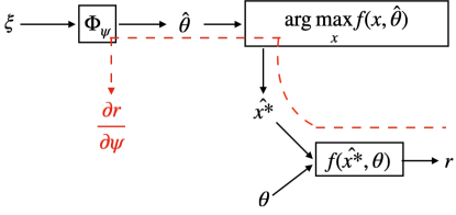
Instead, decision-focused learning directly optimizes with respect to the optimization objective , that is, . The full computational flow is illustrated in Fig.1. In the gradient-based learning, update of ’s gradient is , where utility . The Jacobian is computed implicitly by auto-differentiation of deep learning frameworks (e.g, PyTorch [17]), and is analytical. The main challenge is to compute , which depends on differentiating the operation. One recent approach is to rewrite the objective to be convex (by adding a quadratic regularizer if necessary), build and differentiate the optimality conditions (e.g., KKT conditions) [18] which map to the solution , and then apply implicit function theorem to obtain . Alternatively, in this paper we propose a novel approach that rewrites the problem as an unconstrained problem with soft constraints and derives analytical solutions, based on our observations on the real-world problem structures and coefficient properties.
3 Methodology
Our main idea is to derive a surrogate function for with a closed-form solution such that the Jacobian is analytical, making the computation of gradient straightforward. Unlike other recent work [13, 14, 15, 3], our method does not need to solve KKT optimality condition system. Instead, by adding reasonable costs for infeasibility, we convert the constrained problem into an unconstrained one. With the assumption of concavity, we prove that there exist constant vectors , such that Eq.1 can be equivalently transformed into an unconstrained problem:
| (5) |
The structure of this section is as follows. Section 3.1 proves that the three types of hard constraints can be softened by deriving bounds of ; for this paper, we will assign each entry of the three vectors the equal value (with a slight abuse of notation, we denote for the proofs of bounds; we align with the worst bound applicable to the problem formulation.) Section 3.2 proposes a novel surrogate function of , such that the analytical form of can be easily derived via techniques of implicit differentiation [18] and matrix differential calculus [19] on equations derived by convexity [20]. Based on such derived , we develop our end-to-end learning algorithm of prediction+optimization whose detailed procedure is described in Appendix C.
3.1 Softening the Hard Constraints
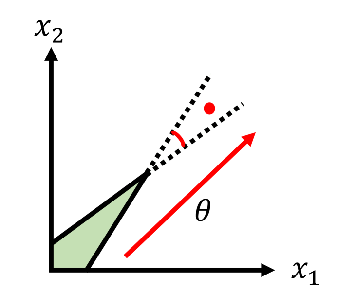
For any hard constraints , we denote its equivalent soft constraints as . should satisfy two conditions: 1) for (feasible ), ; 2) for (infeasible ), is larger than the utility gain(i.e., improvement of the objective value) by violating . Intuitively, the second condition requires a sufficiently large-valued to ensure that the optimization on the unconstrained surrogate objective never violates the original ; to make this possible, we assume that the -norm of the derivative of the objective before conversion is bounded by constant . The difficulty of requirement 2) is that the distance of a point to the convex hull is not bounded by the sum of distances between the point and each hyper-plane in general cases, so the utility gain obtained from violating constraints is unbounded. Fig. 2-(a) shows such an example which features the small angle between hyper-planes of the activated cone. We will refer such kind of ’unbounding’ as "acute angles" below.
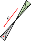
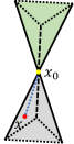
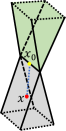
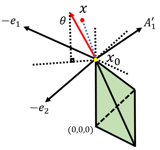
The main effort of this subsection is to analyze and bound the effect caused by such acute angles. Given a convex hull ( is not required here) and any point , let be the nearest point of to , and represent all active constraints at , then all such active constraints must pass through .111Otherwise, there must exist an active constraint and a small neighbourhood of , say , such that , , which implies that either constraint is inactive () or (). The domain is a cone or degraded cone where the tip of the cone is a subspace of . For the rest of the paper, we will call activated cone, as shown in Fig. 2. Note that for any degraded activated cone, is always perpendicular to the tip subspace; therefore, we may project the cone onto the complementary space of the tip and get the same multiplier bound on the projected activated cone with lower dimensions.
Ideally, we aim to eliminate the utility gain obtained from violating with the penalty , i.e., ensure hold for any . For the compactness of symbols and simplicity, we will assume that the main objective is in this section; however note that our proofs apply with the existence of soft constraints and quadratic terms in , which is discussed at the beginning of Appendix A. With such assumption, we now give a crucial lemma, which is the core of our proof for most of our theorem:
Lemma 1.
(Bounding the utility gain) Let be the utility gain, then , where is an infeasible point, the active constraints at , where and are the optimal solution of (i.e., the maximin angle between and any hyperplane of the activated cone ), and the projection of to the tip of cone . is the upper bound of . denotes the angle of two vectors.
Thus, is a feasible choice of , and it suffices by finding the lower bound for . For the rest of the section, we find the lower bound of by exploiting the assumed properties of , e.g., ; we give the explanation of the full proofs for all theoretical results in Appendix A.
3.1.1 Conversion of Inequality Constraints
Let us first consider the constraints , where , . It is easy to prove that given and , the distance of a point to the convex hull is bounded. More rigorously, we have the following theorem, which guarantees the feasibility of softening the hard constraints of inequalities :
Theorem 2.
Assume the optimization objective with constraints , where , and . Then, the utility gain obtained from violating has an upper bound of , where , and is the active constraints.
3.1.2 Conversion of Inequality Constraints
With inequality constraints converted, we now further enforce into soft constraints. It seems that the constraint of this type may form a very small angle to those in . However, as is aligned with the axes, we can augment into soft constraints by proving the following theorem:
Theorem 3.
When there is at least one entry of in the activated cone, the utility gain from deviating the feasible region is bounded by , where is the smallest angle between axes and other constraint hyper-planes and is the union of and .
Hence, we can set . Specially, for binary constraints we may set :
Corollary 4.
For binary constraints where the entries of are either or , the utility gain of violating constraint is bounded by , where or .
which gives a better bound for a set of unweighted item selection problem (e.g. select at most items from a particular subset).
3.1.3 Conversion of Equality Constraints
Finally, we convert into soft constraints. This is particularly difficult, as implies both and , which will almost always cause acute angles. Let’s first consider a special case where there is only one equality constraints and is an element matrix .
Theorem 5.
If there is only one equality constraint (i.e., degrades as a row vector, such like ) and special inequality constraints , , then the utility gain from violating constraints is bounded by , where is the same with theorem 3, is the union of and .
Intuitively, when there is only one equality constraint, the equality constraint can be viewed as an unequal one, for at most one side of the constraint can be in a non-degraded activated cone. Thus, we can directly apply the proof of Theorem 2 and 3, deriving the same bound for .
Finally, we give bounds for general , with as below:
Theorem 6.
Given constraints , , and , where , the utility gain obtained from violating constraints is bounded by , where is the upper bound for eigenvalues of ( is an orthogonal transformation for an -sized subset of normalized row vectors in and ), and is the union of all active constraints from , , and .
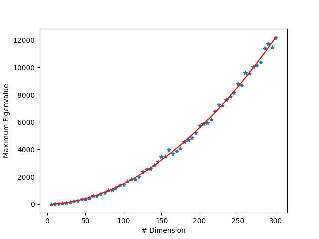
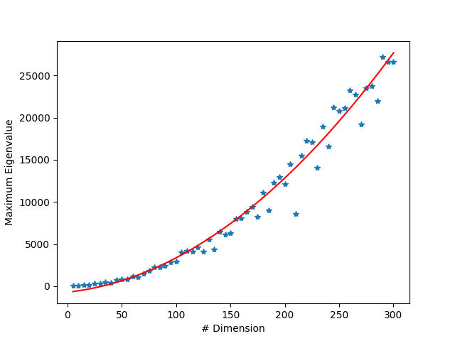
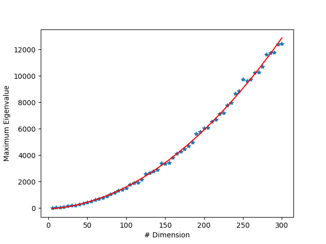
In this theorem, is generated by taking an arbitrary -sized subset from the union of row vectors in and , orthogonizing the subset, and using the orthogonal transformation matrix as ; there are different cases of , and is the upper bound of eigenvalues of over all possible cases of . Note that there are no direct bounds on with respect to and the angles between hyper-planes. However, empirical results (see Appendix A for details) show that for a diverse set of synthetic data distributions, follows. Therefore, empirically we can use a bound for .222For real optimization problems, we can sample from and estimate the largest eigenvalue of . So far, we have proven that all hard constraints can be transformed into soft constraints with bounded multipliers. For compactness, Eq.5 is rewritten in a unified form:
| (6) |
3.2 The Unconstrained Soft Constraints
As Eq.5 is non-differentiable for the operator, we need to seek a relaxing surrogate for differentiation. The most apparent choice of the derivative of such surrogate for is sigmoidal functions; however, it is difficult to derive a closed-form solution for such functions, since sigmoidal functions yield in the denominator, and cannot be directly solved because is not invertible (referring to Appendix B for detailed reasons). Therefore, we have to consider a piecewise roundabout where we can first numerically solve the optimal point to determine which segment the optimal point is on, and then expand the segment to the whole space. To make this feasible, two assumptions must be made: 1) this function must be differentiable, and 2) the optimal point must be unique; to ensure this, the surrogate should be a convex/concave piece-wise function. The second property is for maintaining the optimal point upon segment expansion. Fortunately, there is one simple surrogate function satisfying our requirement:
| (7) |
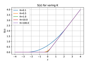
Let and be diagonal matrices as the indicator of , which are and , where is an indicator function. is a hyper-parameter that needs to be balanced. Larger makes the function closer to original; however, if is too large, then the training process would be destabilized, because when the prediction error is large at the start of the training process, might be too steep. Then consider the optimal point for the unconstrained optimization problem maximizing , by differentiaing on both sides, we can obtain:
| (8) |
This equation reveals the closed-form solution of with respect to , and thus the calculation of becomes straightforward:
| (9) |
is invertible as long as at least soft constraints are on the quadratic segment (i.e., active), which is the necessary condition to fix a particular optimal point in . With such solution, we can train our prediction model with stochastic gradient descent (SGD). For each batch of problem instances, we first solve optimization problems numerically using solvers like Gurobi to get the matrix and , and then calculate gradients with the analytical solution. The parameters of the prediction model are updated by such gradients. The sketch of our algorithm is outlined in Appendix C.
4 Applications and Experiments
We apply and evaluate our approach on the three problems described in Section 2, i.e.,linear programming, quadratic programming, and asymmetric soft constraint minimization. These problems are closely related to three applications respectively: synthetic linear programming, portfolio optimization, and resource provisioning, which are constructed using synthetic or real-world datasets. The detailed derivation of gradients for each application can be found in Appendix D.
In our experiments, the performance is measured in regret, which is the difference between the objective value when solving optimization over predicted parameters and the objective value when solving optimization over actual parameters. For each experiment, we choose two generic two-stage methods with -loss and -loss, as well as decision-focused methods for comparison baselines. We choose both SPO+[10] and DF proposed by Wilder et al. [9] for synthetic linear programming and DF only for portfolio optimization,333The method [3] and its variant with dimension reduction [9] have same performance in terms of regret on this problem, thus we choose the former for comparison convenience. as the former is specially designed for for linear objective. For resource provisioning, we use a problem-specific weighted L1 loss, as both SPO+ and DF are not designed for gradients with respect to variables in the soft constraints. All reported results for each method are obtained by averaging on independent runs with different random seeds.
As real-world data is more lenient than extreme cases, in practice we use a much lower empirical bound than the upper bound proved in section 3.1., e.g., constants of around and where is the number of dimensions of decision variables. One rule of thumb is to start from a reasonable constant or a constant times , where such "reasonable constant" is the product of a constant factor (e.g. ) and a roughly estimated upper bound of (which corresponds to in our bounds) with specific problem settings; then alternately increase the constant and time an extra while resetting the constant until the program stops diverging, and the hard constraints are satisfied. In our experiments, we hardly observe situations where such process goes for two or more steps.
4.1 Synthetic Linear Programming
Problem setup. The prediction dataset is generated by a general structural causal model ([21]), ensuring it is representative and consistent with physical process in nature. The programming parameters are generated for various scales in numbers of decision variables, hard constraints, and soft constraints. Full details are given in Appendix E.
Experimental setup. All five methods use the same prediction model – a fully connected neural network of two hidden layers with neurons for each and ReLU [22] for activation. We use AdaGrad [23] as the optimizer, with learning rate and gradient clipped at . We train each method for epochs, and early stop when valid performance degrades for consecutive epochs. Specially, to make DF[9] work right on the non-differentiable soft constraints, we first use black-box solvers to determine whether each soft constraint is active on the optimal point, and then optimize with its local expression (i.e. 2nd-order Taylor expansion at optimal point).
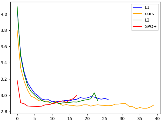
Performance analysis. Our experiments cover four programming problem scales with three prediction dataset sizes. Results are summarized in Table 1. In all cases, our method performs consistently better than two-stage methods, DF and SPO+. Even for the cases with only hard constraints (i.e., the third parameter of problem size is 0), our method still has significant advantage, demonstrating its effectiveness on handling hard constraints. Surprisingly, although the main objective is linear, SPO+ often performs even worse than two-stage methods. Detailed analysis (see the appendix) shows that SPO+ quickly reaches the test optimality and then over-fits. This may be due to that, unlike our method, SPO+ loss is not designed to align with the soft constraints. This unawareness of soft constraint is also why DF is performing worse than our method, as DF is working on an optimization landscape that is non-differentiable at the boundary of soft constraints, on which the optimal point usually lies. Besides, with the increment of the samples in train data, the performance of all methods is improved significantly and the performance gap among ours and two-stage methods becomes narrow, which implies that prediction of two-stage methods becomes better and with lower biases. Even so, our method has better sample efficiency than two-stage methods.
We also investigated effect of the hyper-parameter in our surrogate function, detailed in the appendix. Through our experiments, ’s effect to regret is not monotonic, and its optimal value varies for different problem sizes. Interestingly, ’s effect is approximately smooth. Thus, in practice, we use simple grid search to efficiently find the best setting of .
| Regret (the lower, the better) | ||||||
| Problem Size | L1 | L2 | SPO+ [10] | DF [9] | Ours | |
| 100 | (40, 40, 0) | 2.4540.232 | 2.4930.295 | 2.5060.294 | 2.4780.425 | 2.2580.311 |
| (40, 40, 20) | 2.6260.307 | 2.6640.303 | 2.6670.281 | 2.5360.376 | 2.3500.263 | |
| (80, 80, 0) | 5.7360.291 | 5.8310.361 | 5.7110.309 | 5.7560.317 | 5.2000.506 | |
| (80, 80, 40) | 4.7860.403 | 4.7860.596 | 4.9390.382 | 4.9020.537 | 4.5700.390 | |
| 1000 | (40, 40, 0) | 1.4630.143 | 1.4470.155 | 1.4540.148 | 1.4340.268 | 1.3460.144 |
| (40, 40, 20) | 1.6260.141 | 1.6130.110 | 1.6180.103 | 1.5290.151 | 1.5060.102 | |
| (80, 80, 0) | 3.7680.132 | 3.7180.117 | 3.5730.113 | 3.5320.102 | 3.4310.100 | |
| (80, 80, 40) | 2.9820.176 | 2.9130.172 | 2.8790.148 | 3.3510.212 | 2.7810.165 | |
| 5000 | (40, 40, 0) | 1.0770.105 | 1.0800.109 | 1.0900.105 | 1.0780.092 | 1.0370.100 |
| (40, 40, 20) | 1.2830.070 | 1.2770.077 | 1.2980.077 | 1.2910.091 | 1.2200.071 | |
| (80, 80, 0) | 2.9590.086 | 2.9430.091 | 2.9260.079 | 2.8690.085 | 2.8450.064 | |
| (80, 80, 40) | 2.2390.122 | 2.2240.106 | 2.2340.122 | 2.7480.165 | 2.1720.098 | |
4.2 Portfolio Optimization
Problem and experimental setup. The prediction dataset is daily price data of SP500 from 2004 to 2017 downloaded by Quandl API [24] with the same settings in [3]. We use the same fix as that in linear programming experiment to make DF[9] work with non-differentiable soft constraints, which was also used in [3] for non-convex optimization applications. Most settings are aligned with those in [3], including dataset configuration, prediction model, learning rate (), optimizer (Adam), gradient clip () and number of training epochs (). We set the number of soft constraints to times of , where is the number of candidate equities. For the soft constraint , , where each element of is generated randomly at uniform from ; the elements of matrix is generated independently from , where the probability of is and is . is set as .
Performance analysis. Table 2 summarizes the experimental results. In total, on all problem sizes (#equities), our method performs consistently and significantly better than both two-stage (L1 and L2) methods and the decision focused DF[9]. Among the three baselines, DF is significantly better than two-stage methods, similar to results in [3]. In fact, DF under this setting can be viewed as a variant of our method with infinite and no conversion of softening . The comparison to DF also demonstrates the advantage of our method on processing such non-differentiable cases against the simple 2nd-order Taylor expansion. Besides, with the increment of the number of equities, regrets of all methods decease, which indicates that for the constraint , larger number of equities brings smaller entries of on average (with the presence of , there are many non-zero entries of ), lowering the impact of prediction error for any single entry.
| Regret measured in % (the lower, the better) | ||||
|---|---|---|---|---|
| #Equities | L1 | L2 | DF [9] | ours() |
| 50 | 4.4260.386 | 4.4720.385 | 4.0160.389 | 3.6620.238 |
| 100 | 4.2620.231 | 4.3200.229 | 3.5000.252 | 3.2140.138 |
| 150 | 3.8780.281 | 3.9500.287 | 3.4190.281 | 3.1090.162 |
| 200 | 3.7550.236 | 3.8220.273 | 3.4060.287 | 3.1520.183 |
| 250 | 3.7210.205 | 3.7510.212 | 3.3350.175 | 3.2120.135 |
4.3 Resource Provisioning
Problem setup. We use ERCOT energy dataset [25], which contains hourly data of energy output from 2013 to 2018, data points in total. We use the last samples for test. We aim to predict the matrix , the loads of hours in regions. The decision vairable is -dimensional, and . We test five sets of , with ranging from to .
Experimental setup. We use AdaGrad with learning rate of , and clip the gradient with norm . For the prediction model, we use McElWee’s network [26] which was highly optimized for this task, with -dimensional numerical features and embedding ones as input.
Performance analysis. Table 3 shows the experimental results. The absolute value of regret differs largely across different ratios of . Our method is better than other methods, except for , where the desired objective is exactly -loss and thus performs the best. Interestingly, compared to L1/L2, the Weighted L1 performs better when , but relatively worse otherwise. This is probably due to the dataset’s inherent sample bias (e.g., asymmetric distribution and occasional peaks), which causes the systematic bias (usually underestimation) of the prediction model. This bias exacerbates, when superposed with weighted penalty multipliers which encourage the existing bias to fall on the wrong side. Besides, the large variance for weighted L1 at is caused by a pair of outliers.
| Regret (the lower, the better) | ||||
| L1 | L2 | Weighted L1 | Ours() | |
| 100 | 105.06121.954 | 93.19329.815 | 79.01432.069 | 20.8298.289 |
| 10 | 13.0612.713 | 13.2756.208 | 7.7431.305 | 2.7461.296 |
| 1 | 4.2670.618 | 5.1360.722 | 4.2670.618 | 5.8390.512 |
| 0.1 | 10.8461.606 | 13.6192.195 | 16.4622.093 | 10.2401.248 |
| 0.01 | 99.14521.159 | 118.11229.957 | 230.82591.184 | 94.34129.821 |
5 Related Work
Differentiating / through optimality conditions. For convex optimization problems, the KKT conditions map coefficients to the set of solutions, and thus can be differentiated for using implicit function theorem. Following this idea, existing work developed implicit layers of argmin in neural network, including OptNet [13] for quadratic programs (QP) problems and CVXPY [14] for more general convex optimization problems. Further with linear relaxation and QP regularization, Wilder et al. derived an end-to-end framework for combinatorial programs [9], which accelerates the computation by leverage the low-rank properties of decision vectors [3], and is further extended to mixed integer linear programs in MIPaaL [27]. Besides, for the relaxed LP problems, instead of differentiating KKT conditions, IntOpt [28] proposes an interior point based approach which computes gradients by differentiating homogeneous self-dual formulation.
Optimizing surrogate loss functions. Elmachtoub and Grigas [10] proposed a convex surrogate loss function, namely SPO+, measuring the decision error induced by a prediction, which can handle polyhedral, convex and mixed integer programs with linear objectives. TOPNet [29] proposes a learned surrogate approach for exotic forms of decision loss functions, which however is hard to generalize to handle constrained programs.
Differentiating is critical for gradient methods to optimize decision-focused prediction models. Many kinds of efforts, including regularization for specific problems (e.g., differentiable dynamic programming [30], differentiable submodular optimization [31]), reparameterization [32], perturbation [33] and direct optimization ([12]), are spent for optimization with discrete or continuous variables and still actively investigated.
As a comparison, our work proposes a surrogate loss function for constrained linear and quadratic programs extended with soft constraints, where the soft constraints were not considered principally in previous work. Also, unlike OptNet [13] and CVXPY [15], our method does not need to solve KKT conditions. Instead, by adding reasonable costs for infeasibility, we convert the constrained optimization problem into an unconstrained one while keeping the same solution set, and then derive the required Jacobian analytically. To some degree, we reinvent the exact function [34] in prediction+optimization.
6 Conclusion
In this paper, we have proposed a novel surrogate objective framework for prediction+optimization problems on linear and semi-definite negative quadratic objectives with linear soft constraints. The framework gives the theoretical bounds on constraints’ multipliers, and derives the closed-form solution as well as their gradients with respect to problem parameters required to predict by a model. We first convert the hard constraints into soft ones with reasonably large constant multipliers, making the problem unconstrained, and then optimize a piecewise surrogate locally. We apply and empirically validate our method on three applications against traditional two-stage methods and other end-to-end decision-focused methods. We believe our work is an important enhancement to the current prediction+optimization toolbox. There are two directions for the future work: one is to seek solutions which can deal with hard constraint parameters with negative entries, and the other is to develop the distributional prediction model rather than existing point estimation, to improve robustness of current prediction+optimization methods.
References
- Luo et al. [2020] Chuan Luo, Bo Qiao, Xin Chen, Pu Zhao, Randolph Yao, Hongyu Zhang, Wei Wu, Andrew Zhou, and Qingwei Lin. Intelligent virtual machine provisioning in cloud computing. In Proceedings of IJCAI 2020, pages 1495–1502, 2020.
- Chansombat et al. [2018] Sirikarn Chansombat, Pupong Pongcharoen, and Christian Hicks. A mixed-integer linear programming model for integrated production and preventive maintenance scheduling in the capital goods industry. International Journal of Production Research, 57:1–22, 04 2018. doi: 10.1080/00207543.2018.1459923.
- Wang et al. [2020] Kai Wang, Bryan Wilder, Andrew Perrault, and Milind Tambe. Automatically learning compact quality-aware surrogates for optimization problems. In NeurIPS 2020, Vancouver, Canada, 2020.
- Demirovi et al. [2020] Emir Demirovi, Peter Stuckey, Tias Guns, James Bailey, Christopher Leckie, Kotagiri Ramamohanarao, and Jeffrey Chan. Dynamic programming for predict+optimise. Proceedings of the AAAI Conference on Artificial Intelligence, 34:1444–1451, 04 2020. doi: 10.1609/aaai.v34i02.5502.
- Ganeshapillai et al. [2013] Gartheeban Ganeshapillai, John Guttag, and Andrew Lo. Learning connections in financial time series. In Sanjoy Dasgupta and David McAllester, editors, Proceedings of the 30th International Conference on Machine Learning, volume 28 of Proceedings of Machine Learning Research, pages 109–117, Atlanta, Georgia, USA, 17–19 Jun 2013. PMLR.
- Gurobi Optimization [2021] LLC Gurobi Optimization. Gurobi optimizer reference manual, 2021. URL http://www.gurobi.com.
- Cplex [2020] IBM ILOG Cplex. Release notes for cplex 20.1.0. 2020. URL https://www.ibm.com/docs/en/icos/20.1.0?topic=2010-release-notes-cplex.
- Bengio [1997] Yoshua Bengio. Using a financial training criterion rather than a prediction criterion. Int. J. Neural Syst., 8(4):433–443, 1997. doi: 10.1142/S0129065797000422. URL https://doi.org/10.1142/S0129065797000422.
- Wilder et al. [2019] Bryan Wilder, Bistra Dilkina, and Milind Tambe. Melding the data-decisions pipeline: Decision-focused learning for combinatorial optimization. In The Thirty-Third AAAI Conference on Artificial Intelligence, pages 1658–1665. AAAI Press, 2019.
- Elmachtoub and Grigas [2017] Adam Elmachtoub and Paul Grigas. Smart "predict, then optimize". Management Science, 10 2017. doi: 10.1287/mnsc.2020.3922.
- Donti et al. [2017] Priya L. Donti, Brandon Amos, and J. Zico Kolter. Task-based end-to-end model learning in stochastic optimization. In Proceedings of the 31st International Conference on Neural Information Processing Systems, NIPS’17, page 5490–5500, Red Hook, NY, USA, 2017. Curran Associates Inc. ISBN 9781510860964.
- Song et al. [2016] Yang Song, Alexander Schwing, Richard, and Raquel Urtasun. Training deep neural networks via direct loss minimization. In Proceedings of The 33rd International Conference on Machine Learning, volume 48 of Proceedings of Machine Learning Research, pages 2169–2177, New York, New York, USA, 20–22 Jun 2016. PMLR.
- Amos and Kolter [2017] Brandon Amos and J. Zico Kolter. OptNet: Differentiable optimization as a layer in neural networks. In Doina Precup and Yee Whye Teh, editors, Proceedings of the 34th International Conference on Machine Learning, volume 70 of Proceedings of Machine Learning Research, pages 136–145, International Convention Centre, Sydney, Australia, 06–11 Aug 2017. PMLR. URL http://proceedings.mlr.press/v70/amos17a.html.
- Amos [2019] Brandon Amos. Differentiable Optimization-Based Modeling for Machine Learning. PhD thesis, Carnegie Mellon University, May 2019.
- Agrawal et al. [2019] Akshay Agrawal, Brandon Amos, Shane Barratt, Stephen Boyd, Steven Diamond, and J. Zico Kolter. Differentiable convex optimization layers. In Advances in Neural Information Processing Systems, volume 32, pages 9562–9574. Curran Associates, Inc., 2019.
- Markowitz [1959] Harry M. Markowitz. Portfolio Selection: Efficient Diversification of Investments. Yale University Press, 1959. ISBN 9780300013726. URL http://www.jstor.org/stable/j.ctt1bh4c8h.
- Paszke et al. [2019] Adam Paszke, Sam Gross, Francisco Massa, Adam Lerer, James Bradbury, Gregory Chanan, Trevor Killeen, Zeming Lin, Natalia Gimelshein, Luca Antiga, Alban Desmaison, Andreas Kopf, Edward Yang, Zachary DeVito, Martin Raison, Alykhan Tejani, Sasank Chilamkurthy, Benoit Steiner, Lu Fang, Junjie Bai, and Soumith Chintala. Pytorch: An imperative style, high-performance deep learning library. In H. Wallach, H. Larochelle, A. Beygelzimer, F. d'Alché-Buc, E. Fox, and R. Garnett, editors, Advances in Neural Information Processing Systems 32, pages 8024–8035. Curran Associates, Inc., 2019.
- Griewank and Walther [2008] A. Griewank and A. Walther. Evaluating Derivatives: Principles and Techniques of Algorithmic Differentiation, Second Edition. Other Titles in Applied Mathematics. Society for Industrial and Applied Mathematics (SIAM, 3600 Market Street, Floor 6, Philadelphia, PA 19104), 2008. ISBN 9780898717761.
- Magnus [2019] Jan R. Magnus Jan R. Magnus. Matrix Differential Calculus with Applications in Statistics and Econometrics, Third Edition. Wiley Series in Probability and Statistics. Wiley, 2019. ISBN 9781119541202.
- Boyd and Vandenberghe [2004] Stephen Boyd and Lieven Vandenberghe. Convex Optimization. Cambridge University Press, 2004.
- Peters et al. [2017] Jonas Peters, Dominik Janzing, and Bernhard Schölkopf. Elements of causal inference. The MIT Press, 2017.
- Nair and Hinton [2010] Vinod Nair and Geoffrey E. Hinton. Rectified linear units improve restricted boltzmann machines. In Proceedings of the 27th International Conference on International Conference on Machine Learning, ICML’10, page 807–814, Madison, WI, USA, 2010. Omnipress. ISBN 9781605589077.
- Duchi et al. [2011] John Duchi, Elad Hazan, and Yoram Singer. Adaptive subgradient methods for online learning and stochastic optimization. Journal of Machine Learning Research, 12:2121–2159, 07 2011.
- sp5 [2021] Sp500 data set. 2021. URL https://docs.quandl.com/.
- erc [2021] Ercot data set. 2021. URL https://github.com/kmcelwee/mediumBlog/tree/master/load_forecast/data.
- McElwee [2020] Kevin McElwee. Predict daily electric consumption with neural networks, 2020. URL https://www.brownanalytics.com/load-forecasting.
- Ferber et al. [2020] Aaron Ferber, Bryan Wilder, Bistra Dilkina, and Milind Tambe. Mipaal: Mixed integer program as a layer. In AAAI Conference on Artificial Intelligence, 2020.
- Mandi and Guns [2020] Jayanta Mandi and Tias Guns. Interior point solving for lp-based prediction+optimisation. In H. Larochelle, M. Ranzato, R. Hadsell, M. F. Balcan, and H. Lin, editors, Advances in Neural Information Processing Systems, volume 33, pages 7272–7282. Curran Associates, Inc., 2020.
- Chen et al. [2020] Di Chen, Yada Zhu, Xiaodong Cui, and Carla Gomes. Task-based learning via task-oriented prediction network with applications in finance. In Christian Bessiere, editor, Proceedings of the Twenty-Ninth International Joint Conference on Artificial Intelligence, IJCAI-20, pages 4476–4482. International Joint Conferences on Artificial Intelligence Organization, 7 2020. doi: 10.24963/ijcai.2020/617. URL https://doi.org/10.24963/ijcai.2020/617. Special Track on AI in FinTech.
- Mensch and Blondel [2018] Arthur Mensch and Mathieu Blondel. Differentiable dynamic programming for structured prediction and attention. In 35th International Conference on Machine Learning, volume 80, pages 3459–3468, 2018.
- Djolonga and Krause [2017] Josip Djolonga and Andreas Krause. Differentiable learning of submodular models. In Advances in Neural Information Processing Systems, volume 30, pages 1013–1023. Curran Associates, Inc., 2017.
- Rezende et al. [2014] Danilo Jimenez Rezende, Shakir Mohamed, and Daan Wierstra. Stochastic backpropagation and approximate inference in deep generative models. In Proceedings of the 31st International Conference on International Conference on Machine Learning - Volume 32, ICML’14, page II–1278–II–1286. JMLR.org, 2014.
- Berthet et al. [2020] Quentin Berthet, Mathieu Blondel, Olivier Teboul, Marco Cuturi, Jean-Philippe Vert, and Francis Bach. Learning with differentiable perturbed optimizers. arXiv preprint arXiv:2002.08676, 2020.
- Bertsekas [1997] Dimitri P Bertsekas. Nonlinear programming. Journal of the Operational Research Society, 48(3):334–334, 1997.
Checklist
-
1.
For all authors…
-
(a)
Do the main claims made in the abstract and introduction accurately reflect the paper’s contributions and scope? [Yes]
-
(b)
Did you describe the limitations of your work? [Yes]
-
(c)
Did you discuss any potential negative societal impacts of your work? [Yes]
-
(d)
Have you read the ethics review guidelines and ensured that your paper conforms to them? [Yes]
-
(a)
-
2.
If you are including theoretical results…
-
(a)
Did you state the full set of assumptions of all theoretical results? [Yes]
-
(b)
Did you include complete proofs of all theoretical results? [Yes]
-
(a)
-
3.
If you ran experiments…
-
(a)
Did you include the code, data, and instructions needed to reproduce the main experimental results (either in the supplemental material or as a URL)? [Yes]
-
(b)
Did you specify all the training details (e.g., data splits, hyperparameters, how they were chosen)? [Yes]
-
(c)
Did you report error bars (e.g., with respect to the random seed after running experiments multiple times)? [Yes]
-
(d)
Did you include the total amount of compute and the type of resources used (e.g., type of GPUs, internal cluster, or cloud provider)? [Yes]
-
(a)
-
4.
If you are using existing assets (e.g., code, data, models) or curating/releasing new assets…
-
(a)
If your work uses existing assets, did you cite the creators? [Yes]
-
(b)
Did you mention the license of the assets? [Yes]
-
(c)
Did you include any new assets either in the supplemental material or as a URL? [Yes]
-
(d)
Did you discuss whether and how consent was obtained from people whose data you’re using/curating? [Yes]
-
(e)
Did you discuss whether the data you are using/curating contains personally identifiable information or offensive content? [Yes]
-
(a)
-
5.
If you used crowdsourcing or conducted research with human subjects…
-
(a)
Did you include the full text of instructions given to participants and screenshots, if applicable? [N/A] We did not use crowdsourcing, nor did we conduct research with human subjects.
-
(b)
Did you describe any potential participant risks, with links to Institutional Review Board (IRB) approvals, if applicable? [N/A]
-
(c)
Did you include the estimated hourly wage paid to participants and the total amount spent on participant compensation? [N/A]
-
(a)
Appendix A Mathematical Proofs
Throughout the following proofs, for the convenience of description, we denote two symbols:
-
•
the symbol , which means the angle of two vectors ;
-
•
, which means the conic combination of the row vectors of matrix ; stands for the conic combination of the union of the row vectors of matrix .
Throughout this section, we will assume the same variables as in Eq.1-5 and Section 3 by default, and further make the following assumptions or simplification for ease of description.
-
•
Assume the main objective , where . In reality, elements of the predictive vector have a known range and thus -norm of is bounded by a constant, namely .
-
•
We omit the soft constraints in original objective. Since all proofs in this section consider the worst direction of in Eq.5, for soft constraints which are linear, their derivatives are constant and can be integrated into for any bounded penalty multiplier .
-
•
Similarly, we omit quadratic term . At first glance, it seems that will bring unbounded derivative of decision variable . However, note that we are finding the maximum value of function, and the matrix is semi-definite positive, we have for any . Thus, denote the maximum point of to be , we can find a finite radius , such that any point out of the circle with as the center and as radius is impossible to be the global optimal point; intuitively, the norm of the derivative of becomes so large as to "draw the optimal point back" from too far, and thus we can ignore the points outside the circle. Since the circle is a bounded set, the norm of derivative is also bounded inside the circle.
-
•
When we consider the effect of violating constraints, we only consider non-degraded activated cone, i.e.,, for an activated cone in a -dimensional Euclidean space, there are at least non-redundant active constraints. Otherwise, as we stated in the main paper, we can project the activated cone onto the complementary space of the cone tip (i.e., the solution space of ) and proceed on a low-dimensional subspace.
-
•
As for constraint itself, we assume that for any row vector of in , and any row vector of in , we have and for any row vector , where is the number of constraints. If not, we can first normalize the row vectors of and while adequately scaling , then apply our proofs.
Thus it is straightforward to apply our proofs to the general form of Eq.5.
A.1 Lemma 1
Lemma 1.
(Bounding the utility gain) Let be the utility gain, then , where is an infeasible point, the active constraints at , where and are the optimal solution of (i.e., the maximin angle between and hyperplanes of the activated cone ), and the projection of to the tip of cone . is the upper bound of .
Proof.
The first inequality is trivial as and directly followed from the definition of utility gain .
For the second inequality, by the law of sines, we have , where is the distance of to the -th hyper-plane in the activated cone with (i.e., the -th row of ) being the normal vector of the -th hyper-plane in , and is the angle between -th hyper-plane and . Then the utility gain from violating the constraints follows:
| (10) | ||||
Thus, setting all entries of penalty multiplier in the hard constraint conversion to will give us an upper bound of the minimum feasible . ∎
The rest of the work is to find the lower bound for for any given activated cone and ; as we have assumed , the objective can be equivalently written as444With an abuse of notation, the in Eq.11 represents , as the worst situation for deriving upper bound of is that has the same direction with the objective ’s derivative .
| (11) |
Deriving the lower bound of is the core part of proving Theorem 3 and 6.
A.2 Lemma 7
In order to prove Theorem 2, we give a crucial lemma.
Lemma 7.
Consider a set of hyper-planes with normal vectors , for which forms a cone. Let be the distance of a point to the hyper-plane , where is in the cone of (i.e., , ), then we have .
Proof.
Without loss of generality, let , and (we can scale if ). The distance . Therefore, we have
| (12) | ||||
We next prove that . As , we have
| (13) | ||||
As , must hold. Therefore, . ∎
A.3 Theorem 2
Theorem 2.
Assume the optimization objective with constraints , where , and . Then, the utility gain obtained from violating has an upper bound of , where , and is the active constraints.
Proof.
Let be the vector of distances to the -th hyper-plane of with normal vector from . By definition of and , the distance vector of the point to the convex hull is . When and , obviously Lemma 7 holds. Consider the active constraints which is the subset of active constraints in . The utility gain from violating the rules satisfies:
| (14) | ||||
This holds for any . Therefore, we turn the hard constraint into a soft constraint with penalty multiplier . ∎
A.4 Theorem 3
Theorem 3.
Assume at least one constraint in is active, then the utility gain by deviating from the feasible region is bounded by , where (i.e., the smallest corner between axes and other constraint hyper-planes), and , where and are active constraints in and respectively.
Proof.
As Lemma 1 implies, the key point of proving this theorem is to prove that (the derivative of the objective), is always close to some rows of and .
Consider the activated cone ; all hyper-planes of and violated entries of must pass through ’s tip . Figure 3 gives such an illustrative example. For the rest of the proof, it is enough to assume that the activated cone is a non-degraded cone, since otherwise, as the main paper states, we can project the activated cone onto the supplementary space of its tip. By the projection, we actually reduce the problem to the same one with lower dimensions of , and can apply the following proof in the same way. Let be the number of rows in , i.e., the number of active constraints in ; and be the number of rows in , i.e., the number of active constraints in . Since is non-degraded, we have .
Without loss of generality, we transform the problem equivalently by rearranging the order of dimensions of so that is the first rows of . Let’s see an example after this transformation. As shown in Figure 3, the three solid black vectors are , , and , where the first and second entries of are strictly greater than (otherwise the cone is degraded). Similarly, for the -dimensional non-degraded activated cone, we consider the maximin angle between and all active inequality constraints and (which is equivalent to finding the minimax cosine value of angles between and all active inequality constraints).
Then, guided by Equation 11 in Lemma 1, the upper bound of distance between and hyper-planes with normal vector , is the solution of the following optimization problem w.r.t. and (since the cone is non-degraded, we assume that are linearly independent):
| (15) | ||||
where is the unit vector where the -th entry is and others are . Note that according to our presumptions, , for have already satisfied. The constraints come from the following consideration: if with given we update in an iterative manner such as gradient ascending, would eventually leave current activated cone where (see Figure 3 for an illustration). Since for any dimension index , all entries of and () are non-negative, we know that . To further relax the objective and derive the lower bound, we will assume in the rest of the paper; if , we can simply ignore all in the max operator with .
Given the signs of , we next derive a lower bound of with respect to any given and set of . Now we relax by setting all entries of to , except for the entries with index and to get , where is a permutation of . We have:
| (16) | ||||
where , is the smallest non-zero entry among (and note that and , which means ). The inequalities hold for the relaxation within the operator. Note that the last line of inequality assumes for for the optimal ; otherwise, we can scale further, ignore the index of the optimal point where and proceed with dimensions for the following two facts:
-
1.
term becomes smaller after ignoring such dimension;
-
2.
, which means for any and any vector of the cone we have , and the last line still corresponds to a cone. Therefore the optimal value of last line is no less than ; the removal of term given will not affect the optimal value.
Then, according to the property of minimax, should be equal to ; Otherwise, if is larger than , we can adjust the value of and by a small amount such that the result is better and is still satisfied, which can be repeated until no optimization is possible, and vice versa. With and fixed, the entries of are equal to each other within each group by symmetry.
Therefore, the solution should be in the form of () where , and we have the following set of equations:
| (17) | ||||
With equations in Eq. 17, we get , . As , and as , can be further relaxed to the sine of the smallest angle between axes and the other inequality constraints, and thus we have the lower bound for the optimization problem listed in Equation 16, which is also the cosine lower bound to the nearest normal vector and of the activated cone. This is the denominator of the desired result; the final result follows as we apply such bound to Lemma 1. ∎
A.5 Corollary 4
Corollary 4.
For binary constraints where the entries of (before normalization) are either or , the utility gain of violating constraint is bounded by , where is the same as Theorem 3.
Proof.
The proof of Corollary 4 is almost the same with Theorem 3, except that if the constraint is cardinal, then each entry of is either or . Thus, as all the non-zero entry are the same, we shall replace the third line in Equation 16 with
| (18) |
where is the number of non-zero entry of , each entry being as normalized . By substituting with 555Note in Theorem 3 we have already mentioned the non-positivity of where , thus bigger brings smaller objective., this optimization problem can be further relaxed to
| (19) |
and we can change Equation 17 to
| (20) | ||||
Therefore, similar to the proof of Theorem 3, we get , which leads to the bound , removing the in the denominator. ∎
A.6 Theorem 5
Theorem 5.
If there is only one equality constraint (e.g. ) and special inequality constraints , , then the utility gain from violating constraints is bounded by , where is the same with theorem 3, is the union of active and .666See Theorem 3 for the meaning of union.
Proof.
We first prove the situation where the inequality constraint is only . If we only have one equality constraint, then it can be seen as two separate inequality constraints, which are and ; for any non-degraded activated cone, as and cannot hold simutaneously, there is at most one normal vector of constraint in the activated cone.
If is active (i.e., this constraint is violated, now we have ), then with , the case is exactly the same with Theorem 3. Otherwise, if (i.e., ) is active (i.e., is violated, now ), then the normal vector of the current active constraint is . Note that all other normal vectors of active constraints are (which is the same situation as that in Equation 15 in the proof of Theorem 3, except that is substituted with ); this indicates that the condition of Lemma 7 is satisfied under such scenario. Therefore, we can apply the proof of Theorem 2 in this case and get a better bound than that in the first scenario.
Then, the full theorem is proved as follows: consider any activated cone . For any , and cannot be active simultaneously. If the former is activated, we replace with ; if the latter (or neither) is active, we remain as normal. Then, for this activated cone, the scenario is exactly the same with the situation where the inequality constraints are only . Similarly, if the equality constraint is cardinal, with the same proof of Corollary 4, we can remove the in the denominator.
∎
A.7 Theorem 6
Theorem 6.
Given constraints , , and , where , the utility gain obtained from violating constraints is bounded by , where is the upper bound for eigenvalues of ( is an orthogonal transformation for an -sized subset of normalized row vectors in and ), and is the union of all active constraints from , , and .
Proof.
For any non-degraded activated cone , we have the following optimization problem (it is worth noting that reformulating our original problem to this optimization one is inspired by Equation 11 in Lemma 1):
| (21) | ||||
where is the normal vector of the -th inequality constraints in , is the -th normal vector for the subspace of (and thus represents the same subspace that is represented by the rows of ). According to the assumption, we scale and so that for any . Note that different from the optimization problem stated in Theorem 3, in this problem can be , which means that there can be no entry of active. To get the lower bound of , we may relax the function by keeping the normal vectors in their original direction to where the -th row of satisfies or (the sign of is decided by the direction of ), and thus or (i.e., any pair of elements in will not have opposite signs) for any . Moreover, . We denote the positive as , and the negative as , . Then similar to Theorem 3,
| (22) |
where , . we aggregate , and , into , and get
| (23) |
where , or for any . Therefore, we can further relax by selecting linearly independent vectors that are the closest to the minimum product777The existence of such set of vectors comes from the non-degradation of the activated cone. and ignore the others for the operator, and for the rest of the proof we may assume that .
We will next consider a linear transformation from to that transforms into an orthogonal normal basis. Then we have
| (24) | ||||
where is the maximum eigenvalue of . The row vectors of are . Therefore, our problem has a lower bound of where is the maximum eigenvalue for ; consists of of the vectors in and has the largest maximum eigenvalue for . ∎
Though we do not derive the bound of with respect to the number of dimension and the angle between hyper-planes in the activation cone, we empirically evaluate the behavior of with respect to on randomly generated data. We first generate a normal vector , with each entry generated independently at random from the distribution ; then we generate vectors in with their entries either all not smaller than or all not greater than ; the orthant is chosen with probability . Each entry is independently generated from and shifted by a constant to enforce the signs. We ensure that , by discarding the vectors that do not satisfy such constraint. can be uniform distribution , the distribution for absolute value of normal distribution , or beta distribution . The is then normalized, and we record the largest eigenvalue of , where , is the RQ decomposition of . We repeat times for each and record the mean and maximum eigenvalue for . Below is the result of our evaluation; it shows that the maximum eigenvalue is approximately . See Figure 4,5, and 6 for illustration.
Appendix B Choices of Surrogate Functions
The final goal of surrogate function is to relax the objective with the term , making it differentiable over . Such objective is a piecewise function with respect to with two segments: one is constant with derivative , the other is linear with a constant derivative.
At first glance, sigmoidal surrogates are seemingly the most straightforward candidate for modeling the derivative of such a piecewise function. For a sigmoidal approximation of soft constraints, should satisfy the following four conditions, among which the first two are compulsory, and the third and fourth can be slightly altered (e.g. by setting and remove the fourth condition).
-
1.
When , . should be a small amount, and it serves as a perturbation since otherwise would be always greater than . However, should not be too small to let the optimal point be too far away from the original constraint (for the gradient will reach too late).
-
2.
must be differentiable, and must have a closed-form inverse function.
-
3.
When , , where is constant and very close to . The should cause as small impact as possible when (when there is no waste), and meanwhile it should (very slightly) encourage to grow to the limit instead of discouraging.
-
4.
When , , which means the penalty function has no influence on the clipping border. This condition is important for linear programming; it can be removed for quadratic programming.
To satisfy the conditions above, we need a closed-form sigmoidal function with closed-form inverse function to be , the derivative of the surrogate. Such function can be Sigmoid function (), Tanh/arctan function, or fractional function (, or equivalently ). With the form of confirmed, our function should look like888To satisfy the requirements above, the function needs scaling and translation; we omit them for the simplicity of formulae by simply set , . , with the derivative .
Take , as an example. The optimal point satisfies
| (25) |
Let , , then . can be substituted by any function with sigmoidal function (e.g. , and ) as its derivative. However, is impossible to be invertible, for includes an identity matrix representing and must have strictly more rows than columns if has any other constraint. Therefore, we cannot solve by first solving exactly in a linear system; we need to solve the equation of fractional function, or estimate with pseudo-inverse. Hence, the closed-form solution with sigmoidal surrogate is at least non-attractive.
To derive a closed-form solution for the equation , should be in a simple form (e.g. polynomial form with degrees lower or equal to with respect to ). Unfortunately, no basic function except the sigmoid function can satisfy the conditions listed above; the degree limit makes higher-order Taylor expansion infeasible. Thus, our only choice left is to find a differentiable piecewise function with linear parts on both sides; we shall first solve the optimal point of the surrogate numerically, and extend the segment where the optimal point locates to ; the gradient is correct due to the uniqueness of optimality (which requires a convex surrogate).
Therefore, we choose the function to be
| (26) |
as illustrated in Figure 7, where is a constant. The surrogate is chosen for its simplicity. Not only does such choice satisfy our conditions with minimum matrix computation, but moreover, is linear, which means the equation can be solved in a linear system. The limitation of such method is that it introduces a hyper-parameter to tune: when is large, if the predicted optimal point is far from ground-truth, the gradient will be too large, making the training process instable. On the other hand, if is small, the optimal point may deviate from the feasible region too far, as the hard constraints are not fully enforced within the region . Fortunately, our empirical evaluation shows that the effect of is smooth, and can be tuned by a grid search.
Appendix C Learning and Inference Algorithm
In general, the learning and inference procedures based on our method have the same prediction+optimization workflow as the computational graph we gave in Fig.1. In this section, we propose the detailed algorithm with emphasis on the specific steps in our method.
Alg. 1 is the learning algorithm of stochastic gradient descent in mini-batch. For each sample , it predicts the context variables as (Statement 3) and then solve the program to get the optimal decision variable as (Statement 4). Note that here is solved by solvers such as Gurobi and CPLEX that are capable to get the deterministic optimal solutions. With , the piece of is determined, and thus the surrogate objective . From Statement 5 to 7, we decide the form of surrogate for by first calculating , then use to decide and in the surrogate. is an element-wise indicator function. Specially, if or is the predicted parameter, should be calculated by the predicted value of or ; moreover, in statement 8 we should calculate on the estimated segment, but with ground-truth value of or . In Statement 8, we compute the gradient by back-propagation. Specifically, we directly compute and by their analytical forms, while by auto-grad mechanism of end-to-end learning software such as PyTorch [17], which we use throughout our experiments. Finally, in Statement 9, we update the parameters of with accumulated gradients in this mini-batch.
Alg. 2 is the program with context variable prediction for inference; it is the same with the traditional predict-then-optimize paradigm. Note that the surrogate is no longer needed in this phase.
Appendix D Derivation of Gradients
In this section, we will show the derivation process of the gradient with respect to the three problems stated in the main paper.
D.1 Linear Programming with Soft Constraints
The problem formulation is:
| (27) |
where , and is to be predicted. In this formulation and the respective experiment (synthetic linear programming), we assume that there is no equality constraint.
Let , where is the upper bound of , is the minimum angle between hyper-planes of and the axes. Then, we can write the surrogate as
| (28) | ||||
Calculating the derivative of at the optimal point, we get
| (29) | ||||
This equation gives us the analytical solution of :
| (30) |
Based on such derivative solution of , we differentiate with respect to on both sides:
| (31) | ||||
On the other hand, given real parameter , we calculate the derivative of :
| (32) | ||||
D.2 Portfolio Selection with Soft Constraints
We consider minimum variance portfolio ([16]) which maximizes the return while minimizes risks of variance. The problem formulation is:
| (33) | ||||
where is the decision variable vector – equity weights, is the equity returns, the semi-definite positive is the covariance matrix of returns . Equivalently, we rewrite the constraints of to fit our surrogate framework, as where . Let , and we have surrogate . Then, we may derive the optimal solution and the gradient of with real data with respect to as
| (34) | ||||
Differentiating on both sides of the analytical solution of , we get:
| (35) | ||||
To derive a simplified norm of , let , , . With such notations, we can simplify the previous results to
| (36) |
and the derivative and can be derived as follows:
| (37) | ||||
| (38) | ||||
Let (, ), and finally
| (39) |
D.3 Resource Provisioning
The problem formulation of resource provisioning is
| (40) |
Let , , , , , . Then for the derivative and the analytical solution of , we have
| (41) | ||||
According to the analytical solution of optimal point , the derivative is
| (42) |
For the first term of the derivative above, we have:
| (43) | ||||
Therefore, the simplified result for the first term of the derivative in Equation 42 is:
| (44) |
For the second term, we have:
| (45) |
The simplified second term is thus
| (46) |
Finally, the derivative can be written as
| (47) |
Appendix E Benchmark Details : Dataset and Problem Settings
Our code is public in the repo: https://github.com/PredOptwithSoftConstraint/PredOptwithSoftConstraint.
E.1 Synthetic Linear Programming
E.1.1 Prediction Dataset
We generate the synthetic dataset under a general structural causal model ([21]). In the original form, it is like:
| (48) | ||||
where is the latent variable, observed features of , and the result variable caused by . According to physical knowledge, can be a process of linear, quadratic, or bi-linear form. However, it is difficult to get an explicit form of reasonable . Instead, can be well-represented by deep neural networks.
Thus, alternatively, we use the following generative model:
| (49) | ||||
where behaves as . In our experiment settings, , where each element of is generated randomly at uniform from . We set , where is a matrix whose elements are generated randomly at uniform in , and is applied element-wisely. We implement as a MLP with two hidden layers, and the output is normalized to for each dimension through different data points. Finally, we add a noise of to , where ; and to , where follows a truncated normal distribution which truncates a normal distribution to .
The dataset is split into training, validation and test sets with the proportions , , in respect. The batch size is set to for , for , and for .
E.1.2 Problem Settings
We generate hard constraint , and soft constraint . Each element of or is first generated randomly at uniform within , then set to with probability of . We generate as and . The soft constraint coefficient is generated randomly at uniform from for each dimension.
E.2 Portfolio Optimization
E.2.1 Dataset
The prediction dataset is daily price data of SP500 from 2004 to 2017 downloaded by Quandl API [24] with the same settings in [3]. Most settings are aligned with those in [3], including dataset configuration, prediction model, learning rate (initial with scheduler), optimizer (Adam), gradient clip (), the number of training epochs (), and the problem instance size (the number of equities being ).
E.2.2 Problem Settings
We set the number of soft constraints to times of , where is the number of candidate equities. For the soft constraint , , where each element of is generated randomly at uniform from ; the elements of matrix are generated independently from , where the probability of is and is . is set as .
E.3 Resource Provisioning
E.3.1 Dataset
The ERCOT energy dataset [25] contains hourly data of energy output from 2013 to 2018 with data points. We use the first as the training set, the middle as the validation set, and the last as the test set. We normalize the dataset by dividing the labels by , which makes the typical label becomes value around . We train our model with a batch size of ; each epoch contains batches. We aim to predict the matrix , where represents the following hours and represents the regions, which are . The data is drawn from the dataset of the corresponding region. the decision variable is -dimensional, and .
E.3.2 Problem Settings
We test five sets of , which are , , , , and , against two-stage with -loss, -loss, and weighted -loss. We use AdaGrad as optimizer with learning rate , and clip the gradient with norm . The feature is a -dimensional vector for each matrix ; we adopted McElWee’s Blog [26] for the feature generation and the model. Weighted L1-loss has the following objective:
| (50) |
Note that and are exchanged in the objective. Intuitively, this is because an under-estimation of entries of will cause a larger solution of , which in turn makes larger at test time, and vice versa. Another thing worth noting is that SPO+ cannot be applied to the prediction of the matrix or vector , for it is designed for the scenario where the predicted parameters are in the objective.
Appendix F Supplementary Experiment Results
F.1 Linear Programming with Soft Constraints
The effect of . Table 4 provides the mean and standard deviation of regrets under varying values of . we can see that our method performs better than all other methods with most settings of .
Empirically, to find an optimal for a given problem and its experimental settings, a grid search with roughly adaptive steps suffices. For example,in our experiments, we used a proposal where neighbouring coefficient has difference (e.g. ) works well. Quadratic objective, as in the second experiment, usually requires larger than linear objective as in the first and the third experiment.
| Regret | ||||||
|---|---|---|---|---|---|---|
| Problem Size | ours() | |||||
| 100 | (40, 40, 0) | 2.4230.305 | 2.3780.293 | 2.2650.238 | 2.3010.325 | 2.2580.311 |
| (40, 40, 20) | 2.5300.275 | 2.5740.254 | 2.3840.277 | 2.3210.272 | 2.3500.263 | |
| (80, 80, 0) | 5.2000.506 | 5.5290.307 | 5.6100.351 | 5.5630.265 | 5.5020.353 | |
| (80, 80, 40) | 4.5700.390 | 4.7470.470 | 4.7580.531 | 4.7800.450 | 4.7960.624 | |
| 1000 | (40, 40, 0) | 1.3790.134 | 1.3870.130 | 1.3650.147 | 1.3460.144 | 1.3520.140 |
| (40, 40, 20) | 1.5870.112 | 1.5530.114 | 1.5230.109 | 1.5070.102 | 1.5060.102 | |
| (80, 80, 0) | 3.6170.125 | 3.4310.100 | 3.5400.105 | 3.5130.097 | 3.5070.117 | |
| (80, 80, 40) | 2.7810.165 | 2.8170.167 | 2.8190.155 | 2.8200.157 | 2.8260.197 | |
| 5000 | (40, 40, 0) | 1.0410.094 | 1.0650.098 | 1.0450.099 | 1.0380.102 | 1.0370.100 |
| (40, 40, 20) | 1.2780.072 | 1.2480.076 | 1.2230.075 | 1.2200.071 | 1.2210.074 | |
| (80, 80, 0) | 3.0740.098 | 2.8450.064 | 2.8840.100 | 2.8890.083 | 2.8640.086 | |
| (80, 80, 40) | 2.2170.123 | 2.2220.111 | 2.1720.098 | 2.1740.113 | 2.1770.105 | |
Prediction error. Table 5 and Table 6 are the mean and standard deviation of prediction MSE for all methods. We can find that two-stage methods have an advantage over end-to-end methods on prediction error. however, as demonstrated in our experiments, such advantage does not necessarily lead to the advantage on the regret performance. Surprisingly, although DF[9] works generally on par with other baselines in regret performance, it generates a very large MSE error compared with our method; closer examination suggests that there are some outlier cases where the prediction loss is magnitudes higher than others. Also, the prediction error of DF gets much higher when no soft constraint exists, which is probably because the optimal solution remains the same when all parameters to predict are scaled by a constant factor.
| MSE of | ||||||
|---|---|---|---|---|---|---|
| Problem Size | L1 | L2 | SPO+ | DF | ours () | |
| 100 | (40, 40, 0) | 0.0620.006 | 0.0630.008 | 0.0790.150 | 14.5929.145 | 0.0940.039 |
| (40, 40, 20) | 0.0610.005 | 0.0620.006 | 0.0710.006 | 6.4144.451 | 0.0610.007 | |
| (80, 80, 0) | 0.0580.004 | 0.0590.004 | 0.0660.011 | 28.76813.90 | 0.2470.009 | |
| (80, 80, 40) | 0.0590.004 | 0.0590.004 | 0.0850.008 | 8.98 9.99 | 0.0610.005 | |
| 1000 | (40, 40, 0) | 0.0310.001 | 0.0310.001 | 0.0340.002 | 34.93114.309 | 0.0360.003 |
| (40, 40, 20) | 0.0310.001 | 0.0310.001 | 0.0330.001 | 9.2558.497 | 0.0330.001 | |
| (80, 80, 0) | 0.0300.001 | 0.0290.001 | 0.0320.002 | 90.59035.298 | 0.2220.009 | |
| (80, 80, 40) | 0.0300.001 | 0.0290.001 | 0.0330.001 | 1.0602.395 | 0.0330.002 | |
| 5000 | (40, 40, 0) | 0.0220.000 | 0.0220.000 | 0.0250.001 | 72.08346.685 | 0.0250.001 |
| (40, 40, 20) | 0.0220.000 | 0.0220.000 | 0.2380.001 | 235.789842.939 | 0.2430.001 | |
| (80, 80, 0) | 0.0210.000 | 0.0210.000 | 0.0230.001 | 147.14451.101 | 0.1960.011 | |
| (80, 80, 40) | 0.0200.000 | 0.0200.000 | 0.0220.001 | 0.3720.311 | 0.0240.001 | |
| MSE of | |||||
|---|---|---|---|---|---|
| Problem Size | ours() | ours() | ours() | ours() | |
| 100 | (40, 40, 0) | 0.0680.008 | 0.0910.037 | 0.1880.089 | 0.2040.079 |
| (40, 40, 20) | 0.0940.031 | 0.2040.074 | 0.2440.105 | 0.3430.200 | |
| (80, 80, 0) | 0.1290.049 | 0.2570.182 | 0.6410.476 | 0.8160.351 | |
| (80, 80, 40) | 0.0940.013 | 0.1510.035 | 0.1720.091 | 0.1770.042 | |
| 1000 | (40, 40, 0) | 0.0360.002 | 0.0560.010 | 0.1430.048 | 0.1950.095 |
| (40, 40, 20) | 0.0600.010 | 0.1270.051 | 0.1720.071 | 0.1930.078 | |
| (80, 80, 0) | 0.1140.070 | 0.2200.097 | 1.1240.341 | 1.4070.439 | |
| (80, 80, 40) | 0.0390.002 | 0.0600.006 | 0.0780.010 | 0.0800.008 | |
| 5000 | (40, 40, 0) | 0.0260.001 | 0.0330.004 | 0.0760.025 | 0.0890.037 |
| (40, 40, 20) | 0.0360.004 | 0.0730.019 | 0.1100.038 | 0.1130.026 | |
| (80, 80, 0) | 0.1520.079 | 0.0970.040 | 0.7030.177 | 0.8950.205 | |
| (80, 80, 40) | 0.0260.001 | 0.0320.003 | 0.0380.004 | 0.0400.007 | |
Detailed behaviour of SPO+. As mentioned in the main paper, SPO+ quickly becomes overfited in our experiments, shown by Table 7 as empirical evidence. In our experiments, early stopping starts at epoch , and maximum number of run epochs is ; the results show that SPO+ stops much earlier than other methods under most settings. Figure 8 plots the timely comparison of test performance during training, where SPO+ get overfited quickly, although it performs better in the earlier period of training.
| Average Episode | ||||||
|---|---|---|---|---|---|---|
| Problem Size | L1 | L2 | SPO+ | DF | ours () | |
| 100 | (40, 40, 0) | 20.4610.20 | 12.533.00 | 19.68.58 | 29.5310.24 | 20.5310.39 |
| (40, 40, 20) | 21.479.58 | 14.134.47 | 17.89.98 | 25.4611.41 | 22.4710.29 | |
| (80, 80, 0) | 22.65.78 | 22.68.52 | 20.077.23 | 30.878.83 | 24.538.02 | |
| (80, 80, 40) | 25.28.38 | 24.738.88 | 19.33764 | 249.06 | 28.338.89 | |
| 1000 | (40, 40, 0) | 14.672.61 | 13.21.74 | 102.04 | 27.937.42 | 13.62.53 |
| (40, 40, 20) | 13.22.37 | 13.42.50 | 10.331.40 | 24.68.14 | 10.671.23 | |
| (80, 80, 0) | 19.072.25 | 18.071.83 | 11.872.00 | 25.26.41 | 24.2711.02 | |
| (80, 80, 40) | 19.932.66 | 191.31 | 12.331.95 | 25.49.22 | 17.734.08 | |
| 5000 | (40, 40, 0) | 16.472.59 | 16.271.33 | 11.872.10 | 23.337.34 | 11.82.60 |
| (40, 40, 20) | 17.132.59 | 15.271.79 | 12.82.88 | 21.677.95 | 13.42.77 | |
| (80, 80, 0) | 20.673.20 | 20.82.18 | 13.72.16 | 29.337.22 | 30.079.48 | |
| (80, 80, 40) | 20.472.64 | 212.88 | 12.21.61 | 17.66.84 | 18.535.26 | |
Statistical significance tests. Table 9 shows the results of significance test (one-tailed paired -test), with the assumption that the means of two distributions are the same. The results show that our method is significantly better than other methods under almost all settings.
| -value | |||||
|---|---|---|---|---|---|
| Problem Size | L1 | L2 | SPO+ | DF | |
| 100 | (40, 40, 0) | 3.884 | 4.615 | 5.194 | 1.614 |
| (40, 40, 20) | 5.173 | 5.248 | 6.836 | 1.569 | |
| (80, 80, 0) | 6.024 | 5.661 | 4.523 | 3.610 | |
| (80, 80, 40) | 2.308 | 1.724 | 3.622 | 1.936 | |
| 1000 | (40, 40, 0) | 8.438 | 5.271 | 4.860 | 1.115 |
| (40, 40, 20) | 6.547 | 6.212 | 8.562 | 2.620 | |
| (80, 80, 0) | 12.620 | 10.925 | 7.979 | 2.751 | |
| (80, 80, 40) | 7.116 | 4.465 | 6.223 | 8.230 | |
| 5000 | (40, 40, 0) | 7.130 | 7.808 | 7.546 | 1.175 |
| (40, 40, 20) | 10.410 | 10.238 | 6.555 | 2.382 | |
| (80, 80, 0) | 8.361 | 7.502 | 6.874 | 0.869 | |
| (80, 80, 40) | 6.550 | 4.388 | 5.066 | 11.620 | |
| -value | |||||
|---|---|---|---|---|---|
| Problem Size | L1 | L2 | SPO+ | DF | |
| 100 | (40, 40, 0) | 8.272 | 2.006 | 6.809 | 0.058 |
| (40, 40, 20) | 7.076 | 6.162 | 4.054 | 0.064 | |
| (80, 80, 0) | 1.561 | 2.936 | 2.388 | 5 | |
| (80, 80, 40) | 0.018 | 0.053 | 0.001 | 0.032 | |
| 1000 | (40, 40, 0) | 3.662 | 5.917 | 1.263 | 0.137 |
| (40, 40, 20) | 6.489 | 1.133 | 3.078 | 0.007 | |
| (80, 80, 0) | 2.444 | 1.544 | 7.064 | 0.005 | |
| (80, 80, 40) | 2.600 | 2.667 | 1.114 | 2.937 | |
| 5000 | (40, 40, 0) | 2.545 | 9.074 | 1.342 | 0.125 |
| (40, 40, 20) | 2.834 | 3.487 | 6.406 | 0.012 | |
| (80, 80, 0) | 4.082 | 1.435 | 3.818 | 0.196 | |
| (80, 80, 40) | 6.460 | 3.097 | 8.606 | 1.585 | |
F.2 Portfolio Optimization
Statistical significance tests. Table 10 shows the result of significance test (one-tailed paired -test), with the assumption that the means of two distributions are the same. The results show that our method is significantly better than other methods under every setting.
| -value | -value | |||||
|---|---|---|---|---|---|---|
| #Equities | L1 | L2 | DF | L1 | L2 | DF |
| 50 | 10.329 | 10.628 | 6.141 | 3.213 | 2.186 | 1.279 |
| 100 | 21.414 | 23.995 | 6.200 | 2.125 | 4.495 | 1.157 |
| 150 | 13.402 | 14.503 | 5.690 | 1.119 | 3.971 | 2.789 |
| 200 | 13.617 | 13.104 | 4.329 | 9.086 | 1.500 | 3.465 |
| 250 | 13.904 | 14.483 | 3.205 | 6.915 | 4.044 | 0.003 |
F.3 Resource Provisioning
Statistical significance tests. Table 11 shows the result of significance test (one-tailed paired -test), with the assumption that the means of two distributions are the same.
| -value | -value | |||||
|---|---|---|---|---|---|---|
| L1 | L2 | Weighted L1 | L1 | L2 | Weighted L1 | |
| 100 | 13.133 | 9.357 | 6.429 | 2.914 | 2.115 | 1.576 |
| 10 | 12.484 | 14.231 | 10.897 | 5.622 | 1.493 | 3.190 |
| 0.1 | 1.184 | 5.073 | 11.001 | 0.127 | 8.486 | 1.416 |
| 0.01 | 0.535 | 1.998 | 5.083 | 0.300 | 0.032 | 8.33 |
Appendix G Computing Infrastructure
All experiments are conducted on Linux Ubuntu 18.04 bionic servers with 256G memory and 1.2T disk space with no GPU, for GPU does not suit well with Gurobi.999see Gurobi’s official support website: https://support.gurobi.com/hc/en-us/articles/360012237852-Does-Gurobi-support-GPUs- Each server has 32 CPUs, which are Intel Xeon Platinum 8272CL @ 2.60GHz.
For the first experiment, we use a few minutes to get one set of data 101010Running all methods simultaneously under one particular parameter setting. with training set size , and about hours to get one set of data with training set size . For the second experiment, we use about an hour to get one set of data with , and days to get one set of data with . For the third experiment, we use around hours to obtain one set of data. Though our method is slower to train than two-stage methods, it is 2-3x faster to train than KKT-based decision-focused method.