BSM $B-\bar{B}$ mixing on JLQCD and RBC/UKQCD $N_{f}=2+1$ DWF ensembles

Abstract

We are presenting our ongoing Lattice QCD study on $B-\bar{B}$ mixing on several RBC/UKQCD and JLQCD ensembles with 2+1 dynamical-flavour domain-wall fermions, including physical-pion-mass ensembles. We are extracting bag parameters $B_{B_{d}}$ and $B_{B_{s}}$ using the full 5-mixing-operator basis to study both Standard-Model mixing as well as Beyond the Standard Model mixing, using a fully correlated combined fit to two-point functions and ratios of three-point and two-point functions. Using 15 different lattice ensembles we are simulating a range of heavy-quark masses from below the charm-quark mass to just below the bottom-quark mass.

1 Introduction

Neutral $B_{(s)}$ meson mixing occurs at the one-loop level in the Standard Model (SM) via the box diagrams shown in Fig. 1.

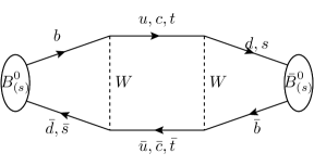
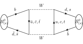
Figure 1: The two $W$-exchange box diagrams contributing to $B-\bar{B}$ mixing. Both are dominated by the $t$ quark loop.

Contributions with a top quark dominate, rendering these processes inherently short-distance. Hence lattice QCD calculations are well suited to determine the non-perturbative contributions due to the strong force, and meson mixing can be expressed in terms of local four-quark operators with $\Delta b=2$. The calculation is similar to the case of $K-\bar{K}$ mixing, which the RBC/UKQCD collaboration has studied extensively [1, 2, 3, 4, 5]. $B_{(s)}-\bar{B}_{(s)}$ mixing, however, faces the additional challenge to simulate the much heavier $b$-quarks. In the past we considered $b$ quarks in the static limit [6, 7], but more recently moved to a fully relativistic setup [8]. Building upon [8] we report here on recent extensions: 1) We consider the full basis with five operators needed in some extensions of the SM. 2) We are working towards a fully non-perturbative renormalisation (NPR) [9] using the RI-SMOM scheme [10]. 3) Measurements on additional ensembles are included extending the range of heavy-quark masses simulated and giving us a better handle to estimate systematic uncertainties.

This will enable us to determine from first principles several quantities which provide stringent tests of the SM or constrain Beyond the Standard Model (BSM) physics. A simple example is the comparison of experimental and theoretical determinations of the mass differences of the neutral $B_{(s)}$ mesons, $\Delta M_{d}$ and $\Delta M_{s}$. HFLAV [11] provides the precise average of the experimental results [12, 13, 14, 15, 16, 17, 18, 19] and on the lattice HPQCD [20] and Fermilab/MILC [21] have determined $\Delta M_{d}$ and $\Delta M_{s}$. Further determinations based on QCD sum rules [22, 23, 24, 25, 26] exist. Currently this comparison [27] shows a tension between the lattice results. While HPQCD is in agreement with the experimental value [11], Fermilab/MILC is not. Our own work [8] provides so far only the ratio $\Delta M_{d}/\Delta M_{s}$, where renormalisation coefficients cancel.

Our work is based on $N_{f}=2+1$ domain-wall fermion (DWF) [28, 29, 30] gauge field ensembles generated by the RBC/UKQCD [31, 32, 33] and JLQCD [34] collaborations. Some of their properties are listed in Table 1.

	$L/a$	$T/a$	$a^{-1}$ [GeV]	$m_{\pi}$ [MeV]	$m_{\pi}L$	hits $\times N_{\mathrm{conf}}$	collaboration id
a1.7m140	48	96	1.730(4)	139.2	3.9	$48\times 90$	R/U C0
a1.8m340	24	64	1.785(5)	339.8	4.6	$32\times 100$	R/U C1
a1.8m430	24	64	1.785(5)	430.6	5.8	$32\times 101$	R/U C2
a2.4m140	64	128	2.359(7)	139.3	3.8	$64\times 82$	R/U M0
a2.4m300	32	64	2.383(9)	303.6	4.1	$32\times 83$	R/U M1
a2.4m360	32	64	2.383(9)	360.7	4.8	$32\times 76$	R/U M2
a2.4m410	32	64	2.383(9)	411.8	5.5	$32\times 81$	R/U M3
a2.5m230-L	48	96	2.453(4)	225.8	4.4	$24\times 100$	J C-ud2-sa-L
a2.5m230-S	32	64	2.453(4)	229.7	3.0	$16\times 100$	J C-ud2-sa
a2.5m310-a	32	64	2.453(4)	309.1	4.0	$16\times 100$	J C-ud3-sa
a2.5m310-b	32	64	2.453(4)	309.7	4.0	$16\times 100$	J C-ud3-sb
a2.7m230	48	96	2.708(10)	232.0	4.1	$48\times 72$	R/U F1M
a3.6m300-a	48	96	3.610(9)	299.9	3.9	$24\times 50$	J M-ud3-sa
a3.6m300-b	48	96	3.610(9)	296.2	3.9	$24\times 50$	J M-ud3-sb
a4.5m280	64	128	4.496(9)	284.3	4.0	$32\times 50$	J F-ud3-sa

Table 1: List of ensembles used in this work. Both the RBC/UKQCD and the JLQCD ensembles feature three lattice spacings which together range from $a^{-1}=1.7$ GeV down to $a^{-1}=4.5$ GeV. To have a consistent naming convention in our set of ensembles from two collaborations, we introduce a special shorthand notation in the first column which is used throughout this work. For readers familiar with earlier work by the RBC/UKQCD ("R/U") and JLQCD ("J") collaborations, we also list in the last column names previously used by the respective collaborations. The column ‘hits $\times N_{\text{conf}}$’ refers to the number of $Z_{2}$ wall sources placed equidistantly on each configuration.

These ensembles feature pion masses from $m_{\pi}=430$ MeV down to the physical range of $m_{\pi}=139$ MeV and six values of the lattice spacing ranging from $a^{-1}=1.7$ GeV up to $a^{-1}=4.5$ GeV. In addition to the two ensembles at a physical pion mass, there is one dedicated pair to study finite volume effects (all parameters the same but the box size is reduced from $m_{\pi}L=4.4$ down to $m_{\pi}L=3.0$) and two other pairs bracketing the strange quark mass to investigate the effect of the strange sea-quark mass. On all ensembles we simulate multiple heavy-quark masses from below or around $m_{c}$ up to just below $m_{b}$ on the finest JLQCD ensemble with $a^{-1}=4.5$ GeV. By performing a combined analysis in terms of a global fit, we expect excellent control when taking the continuum limit and extrapolating to physical quark masses.

Light and strange quarks are simulated using the same DWF action as was used in the sea sector. Heavy quarks ranging from charm to bottom are simulated using stout-smeared [35] Möbius DWF [36] with parameters $b=1.5$ and $c=0.5$. All our computations are done using the software suites Grid [37] and Hadrons [38].

2 Lattice computation

One ingredient we compute on the lattice are two-point correlation functions of mesons with a light and a heavy quark, and mesons with a strange and a heavy quark. These are given by

$$C_{\Gamma_{1},\Gamma_{2}}^{s_{1},s_{2}}=\sum_{\mathbf{x}}\langle O_{\Gamma_{2}}^{s_{2}}(\mathbf{x},t)O_{\Gamma_{1}}^{s_{1}}(\mathbf{0},0)^{\dagger}\rangle=\sum_{n=0}^{\infty}\frac{M_{\Gamma_{2}n}^{s_{2}}M_{\Gamma_{1}n}^{s_{1}*}}{2E_{n}}(e^{-E_{n}t}\pm e^{-E_{n}(T-t)})\,,$$ (1)

with the energy $E_{n}$ and matrix element $M_{\Gamma_{i}n}^{s_{i}}=\langle X_{n}|O_{\Gamma_{i}}^{s_{i}}|0\rangle$ of the $n^{\mathrm{th}}$ excited meson state $X_{n}$. The $\pm$ sign depends on the choice of interpolation operators

$$O_{\Gamma_{i}}^{s_{i}}(\mathbf{x},t)=\bar{q}_{2}(\mathbf{x},t)\sum_{\mathbf{y}}\omega_{s}(\mathbf{x},\mathbf{y})\Gamma_{i}q_{1}(\mathbf{y},t)\,,$$ (2)

which are defined by their quark content $q_{1},q_{2}$ and their Dirac structure, which we limit to $\Gamma_{i}=\gamma_{5}\equiv P$ (pseudoscalar) and $\Gamma_{i}=\gamma_{0}\gamma_{5}\equiv A$ (temporal component of the axial vector). The smearing operator $\omega_{s}$ is chosen to be either smeared ($S$) or local ($L$) at source and sink of each propagator. We use Gaussian smearing [39, 40, 41] on the coarser a1.7 to a2.4 ensembles, where we have correlation functions $C^{s_{1},s_{2}}$ with $s_{1},s_{2}\in\{SL,SS\}$ for the light and strange propagators (the first entry corresponds to the source, the second to the sink) and $s_{1},s_{2}=LL$ for the heavy-quark propagators. On the finer a2.5 to a4.5 ensembles, we only have two-point functions with local interpolators at both source and sink ($LL$).

We determine the non-perturbative contributions to neutral $B_{(s)}$ meson mixing by implementing the four-quark operators

$$\operatorname{{\mathcal{O}_{\Gamma\Gamma}}}=(\bar{b}_{a}\Gamma d_{a})(\bar{b}_{b}\Gamma d_{b})\,,$$ (3)

and calculate on the lattice three-point correlation functions as schematically shown in Fig. 2.

Figure 2: Sketch of the lattice setup to calculate three-point functions with a four-quark-operator insertion at time $t$. The time separation between the $B_{(s)}^{0}$ and $\bar{B}_{(s)}^{0}$ mesons is $\Delta T$.

These three-point functions are described by

$$C_{3}^{\operatorname{{\mathcal{O}_{\Gamma\Gamma}}}}(t,\Delta T) =\langle P(\Delta T){\operatorname{{\mathcal{O}_{\Gamma\Gamma}}}}(t)\bar{P}^{\dagger}(0)\rangle$$

$$\approx\frac{P_{0}^{2}}{4E_{0}^{2}}\langle X_{0}|{\operatorname{{\mathcal{O}_{\Gamma\Gamma}}}}|X_{0}\rangle e^{-E_{0}\Delta T}\times$$

$$\bigg{[}1+2\frac{P_{1}E_{0}}{P_{0}E_{1}}\frac{\langle X_{0}|{\operatorname{{\mathcal{O}_{\Gamma\Gamma}}}}|X_{1}\rangle}{\langle X_{0}|{\operatorname{{\mathcal{O}_{\Gamma\Gamma}}}}|X_{0}\rangle}e^{-\Delta E\Delta T/2}\cosh\big{[}\Delta E\big{(}t-\Delta T/2\big{)}\big{]}\bigg{]}\,,$$ (4)

with $\Delta E=E_{1}-E_{0}$. In Eq. (4) we truncate the expressions by writing only the ground and the first excited states explicitly. Further we use the shorthand $P_{n}=M_{\Gamma_{5}n}^{s}$ with $s=S$ on the a1.7 to a2.4 ensembles and $s=L$ on the a2.5 to a4.5 ensembles. The mixing operators $\operatorname{{\mathcal{O}_{\Gamma\Gamma}}}$ are

$$\mathcal{O}_{1}=\mathcal{O}_{VV+AA}\,,\ \mathcal{O}_{2}=\mathcal{O}_{VV-AA}\,,\ \mathcal{O}_{3}=\mathcal{O}_{SS-PP}\,,\ \mathcal{O}_{4}=\mathcal{O}_{SS+PP}\,,\ \mathcal{O}_{5}=\mathcal{O}_{TT}\,,$$

where $\mathcal{O}_{1}$ is SM operator and $\mathcal{O}_{2-5}$ are important in several SM extensions [3]. A great advantage of the DWF action is that due to the chiral symmetry the mixing between those operators is minimised: $\mathcal{O}_{1}$ does not mix with the others, $\mathcal{O}_{2}$ mixes only with $\mathcal{O}_{3}$ and $\mathcal{O}_{4}$ mixes only with $\mathcal{O}_{5}$.

3 Fitting strategy

We are interested in the bag parameters

$$B_{i}=\frac{\langle P|\mathcal{O}_{i}|\bar{P}^{\dagger}\rangle}{\langle P|\mathcal{O}_{i}|\bar{P}^{\dagger}\rangle_{VSA}}\,,$$ (5)

which are defined as the ratio of a three-point-function matrix element over its vacuum-saturation approximation (VSA). At leading order the SM bag parameter is given by

$$B_{1}=\frac{\langle P|\mathcal{O}_{1}|\bar{P}^{\dagger}\rangle}{8/3m_{P}^{2}f_{P}^{2}}\,,$$ (6)

with meson mass $m_{P}$ and decay constant $f_{P}$. The other bag parameters are

$$B_{i}=\frac{(m_{q}^{2}+m_{h}^{2})\langle P|\mathcal{O}_{i}|\bar{P}^{\dagger}\rangle}{N_{i}m_{P}^{4}f_{P}^{2}}$$ (7)

with quark masses $m_{q}\in\{m_{l},m_{s}\},m_{h}$ and the normalisation factors $N_{2}=-5/3,N_{3}=1/3,N_{4}=2,N_{5}=2/3$ [3]. The product of two two-point functions

$$C_{\Gamma_{1},\Gamma_{2}}(t)C_{\Gamma_{3},\Gamma_{4}}(\Delta T-t) \approx\frac{M_{\Gamma_{2}0}M_{\Gamma_{1}0}M_{\Gamma_{4}0}M_{\Gamma_{3}0}}{4E_{0}^{2}}e^{-E_{0}\Delta T}\times$$

$$\bigg{[}1+\frac{E_{0}}{E_{1}}\bigg{(}\frac{M_{\Gamma_{2}1}M_{\Gamma_{1}1}}{M_{\Gamma_{2}0}M_{\Gamma_{1}0}}+\frac{M_{\Gamma_{4}1}M_{\Gamma_{3}1}}{M_{\Gamma_{4}0}M_{\Gamma_{3}0}}\bigg{)}e^{-\Delta E\Delta T/2}\cosh\big{[}\Delta E\big{(}t-\Delta T/2\big{)}\big{]}\bigg{]}\,,$$ (8)

has a very similar time behaviour to the three-point functions defined in Eq. (4). We have omitted the smearing index in the matrix elements $M_{\Gamma i}^{s_{i}}$, which are chosen to cancel the overlap factors of the corresponding three-point function. This leads to the definition of ratios

$$R_{1}(t,\Delta T) =\frac{C_{3}^{\mathcal{O}_{1}}(t,\Delta T)}{8/3C_{PA}(t)C_{AP}(\Delta T-t)}\,,$$ (9)

$$R_{i}(t,\Delta T) =\frac{C_{3}^{\mathcal{O}_{i}}(t,\Delta T)}{N_{i}C_{PP}(t)C_{PP}(\Delta T-t)}\,,\phantom{aa}2\leq i\leq 5\,,$$ (10)

which have a very good overlap with the bag parameters. In both Eq. (4) and Eq. (8), the $\cosh$-term is equal to $1$ for $t=\Delta T/2$, so that we can define $R_{i}(\Delta T)\equiv R_{i}(t=\Delta T/2,\Delta T)$. We have explored several strategies to extract the bag parameters from the two-point and three-point functions and have settled on a single, fully correlated, combined fit to

$$C_{PP}^{LL},C_{PA}^{LL},C_{AA}^{LL},R_{i}(\Delta T)$$

for each individual bag parameter on the a2.5 to a4.5 ensembles. We have not performed the combined fits to the a1.7 to a2.4 ensembles yet, but we are planning to perform a similar combined fit to

$$C_{PP}^{SS},C_{PA}^{SS},C_{AA}^{SS},C_{PP}^{SL},C_{PA}^{SL},C_{AA}^{SL},R_{i}(\Delta T)$$

on those. To achieve a fully correlated fit in the two-point functions, we are thinning out the correlation function above a transition value $t^{\mathrm{inter}}$ and use only every $3\mathrm{rd}$ timeslice up to the end of the fitrange $t^{\mathrm{max}}$. From the minimum fit timeslice $t^{\mathrm{min}}$ up to $t^{\mathrm{inter}}$, all timeslices are used. We observe that thinning leads to a better conditioned covariance matrix and more stable correlated fits. For the ratios $R_{i}(\Delta T)$ we fit all the data we have available in a range $[\Delta T^{\mathrm{min}},\Delta T^{\mathrm{max}}]$, which effectively corresponds to a thinning in the $\Delta T$ direction, as we have measured the three-point functions only for a subset of $\Delta T$ (typically every $4^{\mathrm{th}}$ value, but on a2.7m230 on every $2^{\mathrm{nd}}$). An example fit of the lightest heavy-light meson on the a4.5m280 for the SM bag parameter ensemble is shown in Fig. 3. The figure also shows the correlation matrix corresponding to the fit, which shows that the ratios and the two-point functions are nicely decorrelated, making this combined fit possible. Earlier attempts to fit the two-point functions directly combined with the raw three-point functions were unstable due to too strong correlations between them.

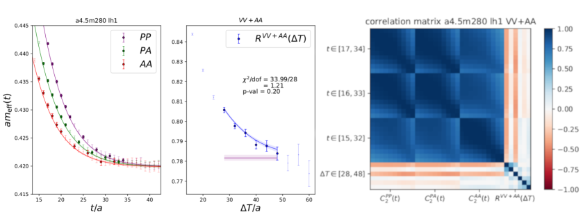
Figure 3: Data and reconstructed fit function of the lightest heavy-light meson on the a4.5m280 ensemble for the SM mixing operator $\mathcal{O}_{1}$. The left panel shows the three two-point functions, the middle panel shows the ratio of three-point and two-point functions, with the purple fit band showing the bag parameter obtained from the fit. Data points shown in bold are the ones actually used in the fit. In the two point function, all data points between $t^{\mathrm{min}}$ and a transition time slice $t^{\mathrm{inter}}$ are taken into account, above that only every $3\mathrm{rd}$ up to $t^{\mathrm{max}}$. Only one $\chi^{2}/$dof value is quoted as this is a single, correlated, combined fit to all data shown on both panels. The right panel shows the corresponding correlation matrix, where the large blue square on the top left belongs to the three two-point functions, which nicely decouple their correlations from the ratios.

We do a fit like this on each ensemble and for every meson (heavy-light and heavy-strange for $4-6$ different heavy masses on each ensemble) and for all five mixing operators. In all cases we can choose fit ranges yielding a good correlated $\chi^{2}/$dof. The RBC/UKQCD ensembles (a1.7, a1.8, a2.4, a2.7) are tuned to be at the physical strange-quark mass. On the JLQCD ensembles, we have two pairs of ensembles (a2.5m310-a/b and a3.6m300-a/b) which differ only in their strange-quark mass, and we interpolate to the physical value using $2m_{K}^{2}-m_{\pi}^{2}$. We find that the effect of the different $m_{s}$ in those ensembles is mild. We show the fit results for the ratio of decay constants $f_{B_{s}}/f_{B_{l}}$ and the ratio of bag parameters $B_{B_{s}}/B_{B_{l}}$ in Fig. 4.

Figure 4: Ratios of decay constants $f_{B_{s}}/f_{B_{l}}$ in the top panel and ratio of bag parameters $B_{B_{s}}/B_{B_{l}}$ in the bottom panel, both for the SM operator $\mathcal{O}_{1}$, plotted against the inverse heavy-heavy pseudoscalar mass as a proxy for the heavy-quark mass. The left vertical green line is at the physical $\eta_{b}$ and the right vertical line at the physical $\eta_{c}$. Only the JLQCD data (a2.5, a3.6, a4.5) is fitted with the combined fit described in the text. The RBC/UKQCD data (a1.7, a1.8, a2.4, a2.7) is the data from [8], which used a different fit method. Using the method described here also for all ensembles is currently being worked on. In the $SU(3)$ symmetric limit ($m_{\pi}\to m_{K}$) these ratios are expected to be $1$, and ensembles closer to the physical $m_{\pi}$ can be seen to have ratios further away from $1$. At least in the $f_{B_{s}}/f_{B_{l}}$ ratio, discretisation effects are small, as can be seen by comparing the red a1.7m140 and orange a2.4m140 data.

This figure illustrates the far reach in the heavy-quark mass possible within our setup, which is facilitated, in particular, through the inclusion of the JLQCD ensembles with very fine lattice spacings. In both ratios, the heavy-quark mass dependence is very mild for every ensemble. We quote the ratios and not the individual decay constants or bag parameters as the NPR is not finalised yet. We also show the bare matrix elements $\langle P|\mathcal{O}_{i}|\bar{P}\rangle$ for the BSM operators in Fig. 5.

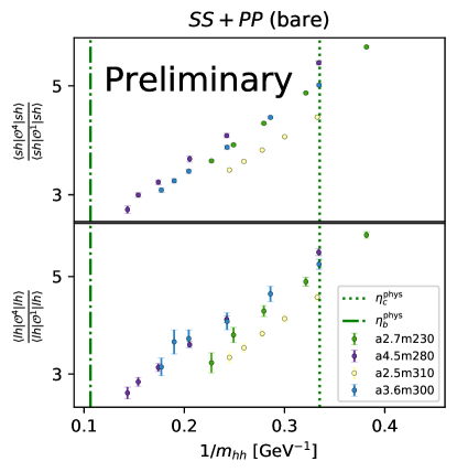
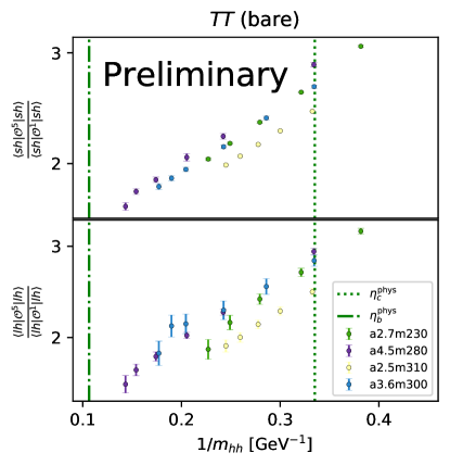
Figure 5: Ratio of matrix elements with BSM operators $O_{2}$–$O_{5}$ over the matrix element with the SM operator $O_{1}$. The top panels show the ratios for strange-heavy mesons, and the bottom panels show the ratios for light-heavy mesons.

4 Conclusion

We have presented our progress towards a complete determination of $B-\bar{B}$ mixing matrix elements on DWF lattices from the JLQCD and RBC/UKQCD collaborations. Our set of ensembles allows us to control all relevant limits in a combined global fit: Two ensembles are at the physical pion mass, a pair of ensembles to study finite-volume effects and in total six different lattice spacings all the way up to $a^{-1}=4.5$ GeV. The heavy-quark masses range from below the physical charm-quark mass to about three-quarters of the bottom-quark mass. We are working on a fully non-perturbative renormalisation using the Rome-Southampton method in the RI-SMOM scheme. On each individual ensemble, a fully correlated, combined fit to two-point functions and ratios of three-point over two-point functions allows us to extract all relevant data with a single $\chi^{2}/$dof for each of the five mixing operators.

References

- [1] RBC/UKQCD collaboration, JHEP 11 (2016) 001 [1609.03334].
- [2] RBC/UKQCD collaboration, PoS LATTICE2016 (2016) 397 [1703.00392].
- [3] RBC/UKQCD collaboration, JHEP 10 (2017) 054 [1708.03552].
- [4] P. Boyle, N. Garron, J. Kettle, A. Khamseh and J. T. Tsang, EPJ Web Conf. 175 (2018) 13010 [1710.09176].
- [5] P. Boyle, N. Garron, R. J. Hudspith, A. Jüttner, J. Kettle, A. Khamseh et al., PoS LATTICE2018 (2019) 285 [1812.04981].
- [6] C. Albertus et al., Phys. Rev. D 82 (2010) 014505 [1001.2023].
- [7] Y. Aoki, T. Ishikawa, T. Izubuchi, C. Lehner and A. Soni, Phys. Rev. D 91 (2015) 114505 [1406.6192].
- [8] RBC/UKQCD collaboration, 1812.08791.
- [9] G. Martinelli, C. Pittori, C. T. Sachrajda, M. Testa and A. Vladikas, Nucl. Phys. B 445 (1995) 81 [hep-lat/9411010].
- [10] C. Sturm, Y. Aoki, N. H. Christ, T. Izubuchi, C. T. C. Sachrajda and A. Soni, Phys. Rev. D 80 (2009) 014501 [0901.2599].
- [11] HFLAV collaboration, Eur. Phys. J. C 81 (2021) 226 [1909.12524].
- [12] ARGUS collaboration, Phys. Lett. B 192 (1987) 245.
- [13] CDF collaboration, Phys. Rev. Lett. 97 (2006) 242003 [hep-ex/0609040].
- [14] LHCb collaboration, Phys. Lett. B 709 (2012) 177 [1112.4311].
- [15] LHCb collaboration, Eur. Phys. J. C 72 (2012) 2022 [1202.4979].
- [16] LHCb collaboration, Phys. Lett. B 719 (2013) 318 [1210.6750].
- [17] LHCb collaboration, New J. Phys. 15 (2013) 053021 [1304.4741].
- [18] LHCb collaboration, Eur. Phys. J. C 73 (2013) 2655 [1308.1302].
- [19] LHCb collaboration, Phys. Rev. Lett. 114 (2015) 041801 [1411.3104].
- [20] R. J. Dowdall, C. T. H. Davies, R. R. Horgan, G. P. Lepage, C. J. Monahan, J. Shigemitsu et al., Phys. Rev. D 100 (2019) 094508 [1907.01025].
- [21] Fermilab Lattice, MILC collaboration, Phys. Rev. D 93 (2016) 113016 [1602.03560].
- [22] A. G. Grozin, R. Klein, T. Mannel and A. A. Pivovarov, Phys. Rev. D 94 (2016) 034024 [1606.06054].
- [23] A. G. Grozin, T. Mannel and A. A. Pivovarov, Phys. Rev. D 96 (2017) 074032 [1706.05910].
- [24] A. G. Grozin, T. Mannel and A. A. Pivovarov, Phys. Rev. D 98 (2018) 054020 [1806.00253].
- [25] M. Kirk, A. Lenz and T. Rauh, JHEP 12 (2017) 068 [1711.02100].
- [26] D. King, A. Lenz and T. Rauh, JHEP 05 (2019) 034 [1904.00940].
- [27] L. Di Luzio, M. Kirk, A. Lenz and T. Rauh, JHEP 12 (2019) 009 [1909.11087].
- [28] D. B. Kaplan, Phys. Lett. B 288 (1992) 342 [hep-lat/9206013].
- [29] T. Blum and A. Soni, Phys. Rev. D 56 (1997) 174 [hep-lat/9611030].
- [30] T. Blum and A. Soni, Phys. Rev. Lett. 79 (1997) 3595 [hep-lat/9706023].
- [31] RBC/UKQCD collaboration, Phys. Rev. D78 (2008) 114509 [0804.0473].
- [32] RBC/UKQCD collaboration, Phys. Rev. D 93 (2016) 074505.
- [33] P. A. Boyle, L. Del Debbio, A. Jüttner, A. Khamseh, F. Sanfilippo and J. T. Tsang, JHEP 12 (2017) 008 [1701.02644].
- [34] K. Nakayama, B. Fahy and S. Hashimoto, Phys. Rev. D 94 (2016) 054507 [1606.01002].
- [35] C. Morningstar and M. J. Peardon, Phys. Rev. D 69 (2004) 054501 [hep-lat/0311018].
- [36] R. C. Brower, H. Neff and K. Orginos, Comput. Phys. Commun. 220 (2017) 1 [1206.5214].
- [37] P. A. Boyle, G. Cossu, A. Yamaguchi and A. Portelli, PoS LATTICE2015 (2016) 023, https://github.com/paboyle/Grid.
- [38] A. Portelli, https://github.com/aportelli/Hadrons .
- [39] S. Güsken, U. Löw, K.-H. Mütter, R. Sommer, A. Patel and K. Schilling, Physics Letters B 227 (1989) 266.
- [40] C. Alexandrou, F. Jegerlehner, S. Güsken, K. Schilling and R. Sommer, Physics Letters B 256 (1991) 60.
- [41] UKQCD collaboration, Phys. Rev. D 47 (1993) 5128 [hep-lat/9303009].