GCR: Gradient Coreset based Replay Buffer Selection for Continual Learning

Abstract

Continual learning (CL) aims to develop techniques by which a single model adapts to an increasing number of tasks encountered sequentially, thereby potentially leveraging learnings across tasks in a resource-efficient manner. A major challenge for CL systems is catastrophic forgetting, where earlier tasks are forgotten while learning a new task. To address this, replay-based CL approaches maintain and repeatedly retrain on a small buffer of data selected across encountered tasks. We propose Gradient Coreset Replay (GCR), a novel strategy for replay buffer selection and update using a carefully designed optimization criterion. Specifically, we select and maintain a ’coreset’ that closely approximates the gradient of all the data seen so far with respect to current model parameters, and discuss key strategies needed for its effective application to the continual learning setting. We show significant gains (2%-4% absolute) over the state-of-the-art in the well-studied offline continual learning setting. Our findings also effectively transfer to online / streaming CL settings, showing up to 5% gains over existing approaches. Finally, we demonstrate the value of supervised contrastive loss for continual learning, which yields a cumulative gain of up to 5% accuracy when combined with our subset selection strategy.

1 Introduction

The field of continual learning (CL) [1] studies the training of models in an incremental fashion, to generalize across a number of sequentially encountered scenarios or tasks, and to avoid the training & maintenance costs of one-off models. A key challenge in CL is the limited access to data from prior tasks; this results in catastrophic forgetting [2], where training on subsequent tasks may potentially erase information in the model parameters pertaining to previous tasks. Approaches to address catastrophic forgetting include modifications to the loss function (e.g., [3, 4]), to the network architecture (e.g., [5, 6]), and to the training procedure and data augmentation (e.g., [7]). In particular, replay-based continual learning maintains a small data sketch from previous tasks, to be included in the training mix throughout the lifetime learning of the model. Remarkably, as little as 1% of saved historical data, using random sampling, is enough to provide significant gains over other CL approaches [7]. This suggests that sophisticated methods for selecting compact data summaries or coresets may perform much better. However, previous approaches to coreset in continual learning have focused on qualitative/diversity-based criteria [8, 9], or bi-level optimizations with significant computational costs and scaling limitations [10].

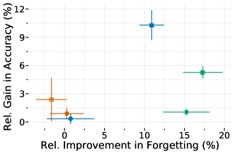
Figure 1: When training CL models on S-Cifar100 with different replay buffer sizes $K\in[200,500,2000]$, the use of replay buffers selected by GCR produces higher model accuracy and lower model forgetting than using reservoir-sampled replay buffers [7]. See text for more details.

We present Gradient-based Coresets for Replay-based CL (GCR), a principled, optimization-driven criterion for selecting and updating coresets for continual learning. Specifically, we select a coreset that approximates the gradient of model parameters over the entirety of the data seen so far. We provide empirical evidence that coresets selected utilizing the above approach mitigate catastrophic forgetting on par with, or better than previous methods. Figure 1 illustrates how our coreset selection approach improves over random data selection by large margins, both in overall accuracy and in retaining of previous tasks. We explore the effect of better representation learning in the CL setting by including a representation learning component [11] into our CL loss function. We conduct extensive experimentation against the state-of-the-art (SOTA) in the well-studied offline CL setting, where the current task’s data is available in entirety for iterative training (2-4% absolute gains over SOTA), as well as the online/streaming setting, where the data is only available in small batches and cannot be revisited (up to 5% gains over SOTA). In particular, we show that the benefit from our coreset selection mechanism increases with increasing number of tasks, showing that GCR scales effectively with task count. Finally, we demonstrate the superiority of GCR over other coreset methods for CL in a head-to-head comparison.

2 Related Work

CL approaches divide broadly into three main themes:
Regularization based approaches preserve learning from earlier tasks via regularization terms placed on model weights (EWC [12], synaptic intelligence [13]), structural regularization [14], or functional regularization [15, 4]). In other work, incremental momentum matching [16] proposes a model-merging step which merges a model trained on the new task with the model trained over the previous tasks, or use knowledge distillation-based regularization [17] to retain learnings from previous tasks.

Architecture adjustments modify model architectures to incorporate CL challenges; for instance, using a recurrent neural network [18], learning overcapacitated deep neural networks in an adaptive way that repeatedly compresses sparse connections [6] or using overlapping convolutional filters [5]. Other work attempts to identify shared information across tasks (CLAW [19]) using variational inference.

Replay based approaches preserve knowledge on previous tasks by storing a small memory buffer of representative data samples from previous tasks for continued training alongside new tasks (ER [20, 21]). Some approaches add a distillation loss to preserve learned representations (iCaRL [22]) or for classifier outputs (DER [7] for points in the buffer. Gradient Episodic Memory (GEM) [23], AGEM) [24]) focuses on minimizing catastrophic forgetting by the efficient use of episodic memory. Meta-Experience Replay (MER) [25] adds a penalty term for between-task interference in a meta-learning framework. Maximally Interfered Retrieval (MIR) method [26] uses controlled memory sampling for replay buffer by retrieving samples that the foreseen model parameters update will most negatively impact. Of these approaches, the distillation loss on the replay buffer [22, 7] show the strongest performance gains at standard CL benchmarks.

Coreset selection: Coresets [27] are small, informative weighted data subsets that approximate specific attributes (e.g., loss, gradients, logits) of original data. Previous work [28, 29] used coresets for unsupervised learning problems such as K-means & K-medians clustering. Coresets enable efficient and scalable Bayesian inference [30, 31, 32, 33, 34] by approximating the model logit sum of the entire data. Several recent works [35, 36, 37, 38, 39] also use coresets to approximate the gradient sum of the individual samples across the entire dataset, for efficient and robust supervised learning. Although coresets are increasingly applied to supervised and unsupervised learning scenarios, the problem of coreset selection for CL is relatively under-studied. We discuss existing coreset based approaches for CL below.
Coresets for Replay-based CL: Approaches include selecting replay buffers by maximizing criteria like sample gradient diversity (GSS [8]), a mix of mini-batch gradient similarity and cross-batch diversity (OCS [9]), adversarial Shapley value(ASER [40]), or representation matching (iCARL [22]). These approaches introduce a secondary selection criterion (to reduce the interference of the current task and forgetting of previous tasks) that is highly specific to each particular approach. As a result, they may not generalize different CL loss criteria. Additionally, previous approaches have not considered weighted replay buffer selection, which increases the representational capabilities of replay buffers. Closest to our work is a recent paper [10] that proposed solving a bi-level optimization for selecting the optimal replay buffer under certain assumptions, rather than for any specified loss function. Their proposal is computationally expensive, intractable in large task scenarios, and scales poorly with buffer size; moreover, they did not compare against recent strong proposals [7]. We compare directly against this approach in our experiments. In contrast to previous coreset approaches in CL, (a) We use an optimization criterion directly tied to the replay loss function used by the CL approach; we show that doing so can achieve better model accuracies across different replay loss functions (ER [25] and DER [7], see Results), (b) We use a weighted coreset selection mechanism for continual learning, where the weights are selected by the coreset optimization criterion and allow effective use of the buffer data.
CL settings: Apart from different learning approaches, CL is also studied under a range of settings, depending on what information and data are available at which stage. In particular, the task-incremental and class-incremental settings assume that task label is known, or not available, respectively, at inference time. In the offline setting, each new task’s data is available in entirety for repeated/ iterative learning [42], whereas online CL only considers data availability in small buffers that cannot be revisited [43].

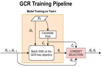
Figure 2: Block diagram showing training, replay buffer selection, and update operations of GCR at time step $t$.

3 Preliminaries

3.1 Notation

We assume that there are $T$ tasks in the continual learning classification problem considered. For each task $t\in\{1,2,\cdots,T\}$, we have an associated dataset $D_{t}$ that is composed of i.i.d data points $\{(x_{it},y_{it})_{i=1}^{|D_{t}|}\}$ where $x_{it}$ is the $i^{th}$ sample and $y_{it}$ is the ground truth label for the $i^{th}$ sample in the dataset $D_{t}$. We assume that each task $t$ is associated with a set of distinct classes $y_{t}={y_{t1},y_{t2},\cdots,y_{tn}}$ and that no tasks have common classes i.e $\underset{t\neq k}{\forall}y_{t}\cap y_{k}=\emptyset$. Let the classifier model be characterized by parameters $\theta$. We split the model parameters into feature extraction layer and linear classification layer. Let the model’s feature extractor output for input sample $x$ is denoted by $\Omega_{\theta}(x)$. The model logits output for input sample $x$ is denoted by $h_{\theta}(x)$ and the predicted probability distribution over the classes for input $x$ is denoted by $f_{\theta}(x)=\textsc{softmax}(h_{\theta}(x))$. We use $t$ to denote the last task observed so far. Let, $l$ be the classification loss function (such as cross-entropy loss).Let the data buffer of previous tasks used for the replay be denoted by $\mathcal{X}$ and $\mathcal{L}_{rep}(\theta,\mathcal{X})$ be the replay-buffer loss over the entire replay buffer $\mathcal{X}$.

3.2 Continual Learning

Following the above notations, the goal of continual learning at step $t$ is to minimize the following objective:

$$\underset{\theta}{\operatorname{argmin\hskip 1.99168pt}}\sum_{i=1}^{t}\sum_{(x,y)\in D_{i}}l(y,f_{\theta}(x))$$ (1)

where $l$ is the cross-entropy loss function.

In a continual learning setup, at step $t$, we only have access to data points from task $t$, making it difficult to optimize the above objective directly. In particular, we have to make sure that while the model is learning on a new task, it should not forget previous tasks.

3.3 Replay-based Continual Learning

Replay-based CL methods maintain a small buffer of data points from previous tasks on which the model is trained and the data samples from the new task to make the model retain the knowledge of previous tasks. Following the notation earlier, we denote the replay buffer of previous tasks by $\mathcal{X}$. One of the possible formulations for replay-based methods for continual learning is as follows:

$$\underset{\theta}{\operatorname{argmin\hskip 1.99168pt}}\sum_{(x,y)\in D_{t}}l(y,f_{\theta}(x))+\lambda\mathcal{L}_{rep}(\theta,\mathcal{X})$$ (2)

where $\mathcal{L}_{rep}$ is the replay loss of the model on samples from replay buffer, and $\lambda$ is a hyperparameter denoting the replay loss coefficient. Early work used cross-entropy for the replay loss (see e.g., ER [20]); however, recent work (Dark Experience Replay, DER [7]), proposes storing the logits ($z$) associated with data points at the time of selection for use in an additional distillation loss. The authors show that DER outperforms a range of previous proposals in both task-incremental and class-incremental offline continual learning scenarios. The DER objective is:

$$\mathcal{L}_{rep}(\theta,\mathcal{X})=\sum_{(x,y)\in\mathcal{X}}\bigg{(}\alpha{\left\|z-f_{\theta}(x)\right\|}^{2}+\beta l(y,f_{\theta}(x))\bigg{)}$$ (3)

4 GCR: Methods

Figure 2 shows the overall GCR workflow. We frame an incremental update process that takes the previously selected replay buffer $\mathcal{X}_{t-1}$ along with a candidate pool $\mathcal{C}_{t}$ from the current task’s data $D_{t}$. We work with the candidate pool $C_{t}$ instead of the task data $D_{t}$ in order to have a more general formulation that covers both Offline CL (all current task data is available) and Online CL (data arrives sequentially in small buffers) scenarios.

Our primary contribution is a formulation of the replay buffer selection as a principled optimization problem based on gradient approximation. We discuss the various components of GCR needed to support this optimization objective, and then sketch how they combine in our overall continual learning framework.

4.1 GradApprox for Replay Buffer Selection

We propose a weighted gradient approximation objective for selecting replay buffers. Given a dataset $D=\{d_{i}\}_{i=1}^{i=|D|}$, associated sample weights $W_{D}=\{w_{i}\}_{i=1}^{i=|D|}$, and a subset size $K$, GradApprox selects a data subset $\mathcal{X}:\mathcal{X}\subset D,|\mathcal{X}|=K$ and its associated weights $W_{\mathcal{X}}$, using the following optimization objective:

$$\underset{\mathcal{X},W_{\mathcal{X}}:\mathcal{X}\subset D,|\mathcal{X}|=K,W_{\mathcal{X}}\geq 0}{\operatorname{argmin}}L_{sub}(D,W_{D},\mathcal{X},W_{\mathcal{X}},\lambda)\text{ where }$$ (4)

$$L_{sub}(D,W_{D},\mathcal{X},W_{\mathcal{X}},\lambda)=\bigg{\|}\sum_{(d,w)\in(D,W_{D})}\nabla_{\theta}l_{rep}(\theta_{t},d,w)$$

$$-\sum_{(\hat{d},\hat{w})\in(\mathcal{X},W_{\mathcal{X}})}\nabla_{\theta}l_{rep}(\theta_{t},\hat{d},\hat{w})\bigg{\|}^{2}+\lambda\left\|W_{\mathcal{X}}\right\|^{2}$$

In the above equation, the replay loss function $l_{rep}$ is a weighted individual sample replay loss. In other words, GradApprox selects a subset of data points, and associated weights, such that the weighted sum of individual samples’ replay loss gradient is closest to the replay loss gradient of the entire dataset. Since this optimization is repeatedly applied after each task, the target of approximation (gradient on $D$) also has weights $W_{D}$ learned from the previous round of GradApprox. Note that the use of weights is a necessary degree of freedom in order to achieve the approximation; i.e., it allows us to feasibly approximate the overall gradient using only a subset of points. Further, these weights must necessarily be used in the subsequent learning algorithm, as the gradient approximation holds only under the conditions of weighted sum with chosen weights.

The above coreset optimization problem is generally applicable to any chosen replay loss function. For instance, using it on the DER [7] replay loss from Equation 3 gives us a general weighted loss: $l_{rep}(\theta,d,w)=\alpha w{\left\|z-h_{\theta}(x)\right\|}^{2}+\beta wl(y,f_{\theta}(x))$, where $d=(x,y,z)$, where the weights are selected by GradApprox. The first loss component is the distillation loss, and the second loss component is the label loss, each scaled by the respective hyperparameters $\alpha$ and $\beta$. Similarly, we can apply GradApprox to the vanilla Experience Replay loss (only cross-entropy on buffer) to improve upon the selected candidate pool for that loss function ([20], also see Table 9 in the supplementary materials). We apply GradApprox to the GCR loss objective, described in the next section.

GradApprox Implementation: Detailed pseudocode of the GradApprox algorithm is given in Algorithm 2. The optimization problem given in Eq (4) is weakly submodular [35, 44]. Hence, we can effectively solve it using a greedy algorithm with approximation guarantees–we use Orthogonal matching pursuit to find the subset and their associated weights. We also added to Eq (4) an $l_{2}$ regularization component over the weights of the replay buffer to discourage large weight assignments to data samples in the selected replay buffer, thereby preventing the model from overfitting on some samples. Finally, we select an equal number of samples from each class to make the selected replay buffer robust to the class imbalance in the dataset. In other words, if there are $C$ classes in the dataset $D$, we solve gradient approximation problems using per-class approximation by selecting a weighted subset of size $\frac{K}{C}$ from the data instances that pertain to the class being considered.

4.2 GCR Loss objective

We adapt and modify the replay loss function from DER [7] (current SOTA in offline continual learning) with the following two goals in mind: (a) to demonstrate the value of GradApprox as a replay buffer selection algorithm and (b) to achieve results, as an overall system, that beats current known SOTA performance in both offline and online continual learning. To use the replay loss from DER [7], for each data sample $(x,y)$ in replay buffer and candidate pool, we also store historical model logit output $z$. Therefore, each data sample in the replay buffer and candidate pool consists of $(x,y,z)$. The formulation of the loss objective $\mathcal{L}(\theta)$ considered by GCR is given below:

$$\mathcal{L}(\theta)=\underbrace{\sum_{(x,y)\in D_{t}}l(y,f_{\theta}(x))}_{\text{(a)}}+$$ (5)

$$\underbrace{\underset{(x^{\prime},y^{\prime},z^{\prime},w^{\prime})\in(\mathcal{X}_{t-1}\mathbin{+\mkern-10.0mu+}{}\mathcal{C}_{t},W_{\mathcal{X}_{t-1}}\mathbin{+\mkern-10.0mu+}{}W_{\mathcal{C}_{t}})}{\sum}\alpha w^{\prime}{\left\|z^{\prime}-h_{\theta}(x^{\prime})\right\|}^{2}}_{\text{(b)}}+$$

$$\underbrace{\underset{(\hat{x},\hat{y},\hat{z},\hat{w})\in(\mathcal{X}_{t-1}\mathbin{+\mkern-10.0mu+}{}\mathcal{C}_{t},W_{\mathcal{X}_{t-1}}\mathbin{+\mkern-10.0mu+}{}W_{\mathcal{C}_{t}})}{\sum}\beta\hat{w}l(\hat{y},f_{\theta}(\hat{x}))}_{\text{(c)}}+$$

$$\underbrace{\underset{(\dot{x},\dot{y},\dot{z},\dot{w})\in(\mathcal{X}_{t-1}\mathbin{+\mkern-10.0mu+}{}\mathcal{C}_{t},W_{\mathcal{X}_{t-1}}\mathbin{+\mkern-10.0mu+}{}W_{\mathcal{C}_{t}})}{\sum}\gamma\dot{w}l_{supcon}(\dot{x},\dot{y},\mathcal{X}_{t-1}\mathbin{+\mkern-10.0mu+}{}\mathcal{C}_{t},\theta)}_{\text{(d)}}$$

where,

$$l_{supcon}(x,y,\mathcal{A},\theta)=$$ (6)

$$\frac{1}{|P(y)|}\sum_{(\dot{x},\dot{y},\dot{z})\in P(y)}\frac{\exp{}(\Omega_{\theta}(\dot{x})\cdot\Omega_{\theta}(x))}{\underset{(\bar{x},\bar{y},\bar{z})\in\mathcal{A}}{\sum}\exp{}(\Omega_{\theta}(\bar{x})\cdot\Omega_{\theta}(x))}$$

$$P(y)=\{(\dot{x},\dot{y},\dot{z})\in\mathcal{A}:\dot{y}=y\}$$

$$\text{and }\mathbin{+\mkern-10.0mu+}{}\text{ is a concatenation operator.}$$

The optimization objective consists of four components. The first component (a) measures prediction loss compared to ground-truth labels for current task data. The second and third components (b, c) measure the current model’s loss computed over data from the combination of replay buffer and current task candidate pool, in terms of distillation loss and label loss, respectively. As outlined in the previous section, GCR uses a weighted loss over the replay buffer, where the weights are an outcome of the replay buffer selection procedure (see previous sections). The fourth and final loss component (d) is a weighted version of supervised contrastive loss [11], initially proposed for standard supervised learning settings. This loss term improves the model’s learned representations by forcing data samples from the same class to be closer in the embedding space than those from other classes. In our work, we always use data samples from the combined candidate pool and replay buffer as anchor points for supervised contrastive learning loss.

DER also uses a loss criterion similar to (a,b,c) above. The primary differences in our loss function compared to DER are (1) the weighted-sum formulation of the loss, with weights selected by GradApprox optimization (our primary contribution), and (2) the use of supervised contrastive loss (d) to further improve the learned model (our secondary contribution). We show in ablation studies that these contributions independently and cumulatively add value over and above current SOTA. We also note that GCR is applicable more broadly, to any specified replay loss funnctions (see e.g., ER [20] based replay loss function, supplementary data C).

Input: Dataset: $D$, Parameters: $\theta$, Scalars: $\alpha$, $\beta$, $\gamma$, $\lambda$, Learning rate: $\eta$, Batch size:$B$, Buffer Size: $K$, Tolerance: $\epsilon$

Output: Parameters: $\theta$

1 Initialize Replay Buffer: $\mathcal{X}=\emptyset$, Replay Buffer weights: $W_{\mathcal{X}}=\emptyset$, and sample count: $n=0$

2 for $D_{t}\in D$  do

3       Initialize Candidate Pool: $\mathcal{C}_{t}=\emptyset$ and task sample count: $n_{t}=0$

4       for $(x,y)\in D_{t}$ do

5             Update task sample count: $n_{t}=n_{t}+1$ and sample count: $n=n+1$

6             $\{(x^{\prime},y^{\prime},z^{\prime},w^{\prime})\}=\operatorname{AdaptiveSampling}(\mathcal{X},\mathcal{C}_{t},n_{t},n)$

7             $x_{aug}=\operatorname{Augment}(x)$, $x^{\prime}_{aug}=\operatorname{Augment}(x^{\prime})$

8             Calculate model logit outputs: $z=h_{\theta}(x_{aug})$

9             $\theta=\theta-\eta\nabla_{\theta}\bigg{(}l(y,f_{\theta}(x_{aug}))+\alpha w^{\prime}{\left\|z^{\prime}-h_{\theta}(x^{\prime}_{aug})\right\|}^{2}+\beta w^{\prime}l(y^{\prime},f_{\theta}(x^{\prime}_{aug}))+\gamma w^{\prime}l_{supcon}(x^{\prime}_{aug},y^{\prime},\mathcal{X}\mathbin{+\mkern-10.0mu+}{}\mathcal{C},\theta)\bigg{)}$

10             $\mathcal{C}=\operatorname{Reservoir}(\mathcal{C},(x,y,z),K)$

11            

12      $\mathcal{X},W_{\mathcal{X}}=\operatorname{GradApprox}(\mathcal{X}\mathbin{+\mkern-10.0mu+}{}\mathcal{C}_{t},W\mathbin{+\mkern-10.0mu+}{}\mathbbm{1},\theta,\lambda,K,\epsilon)$

13

Algorithm 1 GCRAlgorithm

Input: Dataset: $D=\{(x_{i},y_{i},z_{i})\}_{i=1}^{n}$, Existing Weights: $D_{w}$, Parameters: $\theta$, Scalar: $\lambda$, Budget: $K$, Tolerance: $\epsilon$

Output: Subset: $\mathcal{X}$, Subset Weights: $\mathcal{X}_{w}$

1 Initialize $Y=\operatorname{LabelCount}(D)$

2 Partition dataset $D$: $D=\{D_{y}\}_{y=1}^{Y}$

3 Partition dataset weights $W_{D}$ based on the labels of data samples: $W_{D}=\{W_{D_{y}}\}_{y=1}^{Y}$

4 Initialize Replay Buffer: $\mathcal{X}=\emptyset$ and Replay Buffer weights: $\mathcal{X}_{w}=\emptyset$

5

6for $y\in\{1,2,\cdots,Y\}$ do

7       Initialize PerClass budget: $k_{y}=\frac{K}{Y}$, PerClass subset: $\mathcal{X}_{y}=\emptyset$ and PerClass weights: $W_{\mathcal{X}_{y}}=\mathbf{0}$

8       Calculate residuals : ${r}=\nabla_{\mathbf{w}}L_{sub}(D_{y},D_{yw},\mathcal{X}_{y},\mathbf{w},\lambda)|_{\mathbf{w}=\mathcal{X}_{yw}}$

9       while $|\mathcal{X}_{y}|\leq k_{y}$ and $L_{sub}(D_{y},W_{D_{y}},\mathcal{X}_{y},W_{\mathcal{X}_{y}},\lambda)\geq\epsilon$ do

10             Find out maximum residual element: $e=\underset{j}{\text{argmax }}|r_{j}|$

11             Update PerClass subset: $\mathcal{X}_{y}=\mathcal{X}_{y}\cup\{e\}$

12             Calculate updated weights: $W_{\mathcal{X}_{y}}=\underset{\mathbf{w}}{\text{argmin }}L_{sub}(D_{y},W_{D_{y}},\mathcal{X}_{y},\mathbf{w},\lambda)$

13             Calculate residuals : ${r}=\nabla_{\mathbf{w}}L_{sub}(D_{y},W_{D_{y}},\mathcal{X}_{y},\mathbf{w},\lambda)|_{\mathbf{w}=W_{\mathcal{X}_{y}}}$

14            

15      Update subset: $\mathcal{X}=\mathcal{X}\mathbin{+\mkern-10.0mu+}{}\mathcal{X}_{y}$ and subset weights: $W_{\mathcal{X}}=W_{\mathcal{X}}\mathbin{+\mkern-10.0mu+}{}W_{\mathcal{X}_{y}}$

Algorithm 2 GradApprox Algorithm

Further optimization: The candidate set for the current task is selected by reservoir sampling, specifically in order to maintain candidate data points alongside intermediate logits for the distillation loss in the GCR objective. It is possible to improve the candidate pool selection process further through a gradient-approximation objective at the end of current task training. However, this strategy would require maintaining intermediate logits for the entire dataset, requiring prohibitive storage requirements.

4.3 The GCR algorithm

We now put together the various components described above in a continual learning workflow. The pictorial representation of the GCR algorithm was presented in Figure 2 and its detailed pseudocode in Algorithm 1. At each step GCR trains the model on the current task data, and updates the replay buffer with a weighted summary of size $K$ selected from the candidate pool $\mathcal{C}_{t}$ and the previous replay buffer $\mathcal{X}_{t-1}$.

$$\mathcal{X}_{t},W_{\mathcal{X}_{t}}=\operatorname{GradApprox}(\mathcal{X}_{t-1}\mathbin{+\mkern-10.0mu+}{}\mathcal{C}_{t},W_{\mathcal{X}_{t-1}}\mathbin{+\mkern-10.0mu+}{}W_{\mathcal{C}_{t}},\theta,K)$$ (7)

Each point in the candidate pool is initially assigned unit weight; i.e., $W_{\mathcal{C}_{t}}=\mathbbm{1}$. As shown in the pseudocode, we employ reservoir sampling [45] for selecting the candidate pool. We also use adaptive sampling described in Algorithm 3 to sample tasks from the combined candidate pool and the replay buffer. Due to space constraints, we give detailed pseudocode of the Adaptive Sampling Algorithm in Supplementary materials A. Finally, the pseudocode given in Algorithm 1 requires the knowledge of task boundaries to update replay buffer using GradApprox; however, we can also use streaming boundaries or regular intervals of data samples as boundaries in practice to implement the GCR algorithm, thereby making it task agnostic.

5 Experiment setup

We test the efficacy of our approach GCR by comparing its performance with different state-of-the-art continual learning baselines under different CL settings.

		S-Cifar-10			S-Cifar-100			S-TinyImageNet
Setting	Method	K=200	K=500	K=2000	K=200	K=500	K=2000	K=200	K=500	K=2000
Class-IL	ER	49.16±2.08	62.03±1.70	77.13±0.87	21.78±0.48	27.66±0.61	42.80±0.49	8.65±0.16	10.05±0.28	18.19±0.47
	GEM	29.99±3.92	29.45±5.64	27.2±4.5	20.75±0.66	25.54±0.65	37.56±0.87	-	-	-
	GSS	38.62±3.59	48.97±3.25	60.40±4.92	19.42±0.29	21.92±0.34	27.07±0.25	8.57±0.13	9.63±0.14	11.94±0.17
	iCARL	32.44±0.93	34.95±1.23	33.57±1.65	28.0±0.91	33.25±1.25	42.19±2.42	5.5±0.52	11.0±0.55	18.1±1.13
	DER	63.69±2.35	72.15±1.31	81.00±0.97	31.23±1.38	41.36±1.76	55.45±0.86	13.22±0.92	19.05±1.32	31.53±0.87
	GCR	64.84±1.63	74.69±0.85	83.97±0.58	33.69±1.4	45.91±1.3	60.09±0.72	13.05±0.91	19.66±0.68	35.68±0.52
Task-IL	ER	91.92±1.01	93.82±0.41	96.01±0.28	60.19±1.01	66.23±1.52	74.67±1.2	38.83±1.15	47.86±0.87	62.04±0.7
	GEM	88.67±1.76	92.33±0.8	94.34±1.31	58.84±1.0	66.31±0.86	74.93±0.6	-	-	-
	GSS	90.0±1.58	91.73±1.18	93.54±1.32	55.38±1.34	60.28±1.18	66.88±0.88	31.77±1.34	36.52±0.91	43.75±0.83
	iCARL	74.59±1.24	75.63±1.42	76.97±1.04	51.43±1.47	58.16±1.76	67.95±2.69	22.89±1.83	35.86±1.07	49.07±2.0
	DER	91.91±0.51	93.96±0.37	95.43±0.26	63.09±1.09	71.73±0.74	78.73±0.61	42.27±0.9	53.32±0.92	64.86±0.48
	GCR	90.8±1.05	94.44±0.32	96.32±0.18	64.24±0.83	71.64±2.1	80.22±0.49	42.11±1.01	52.99±0.89	66.7±0.59

Table 1: Offline Class-IL and Task-IL Continual Learning. See text for details. Numbers represent mean ± SEM of model test accuracy over 15 runs. Best-performing models in each column are bolded (paired $t$-test, $p<0.05$). Subsequent tables follow the same style.

		S-Cifar-10			S-Cifar-100			S-TinyImageNet
Setting	Method	K=200	K=500	K=2000	K=200	K=500	K=2000	K=200	K=500	K=2000
Class-IL	DER	35.79±2.59	24.02±1.63	12.92±1.1	62.72±2.69	49.07±2.54	28.18±1.93	64.83±1.48	59.95±2.31	39.83±1.15
	GCR	32.75±2.67	19.27±1.48	8.23±1.02	57.65±2.48	39.2±2.84	19.29±1.83	65.29±1.73	56.4±1.08	32.45±1.79
Task-IL	DER	6.08±0.7	3.72±0.55	1.95±0.32	25.98±1.55	25.98±1.55	7.37±0.85	40.43±1.05	28.21±0.97	15.08±0.49
	GCR	7.38±1.02	3.14±0.36	1.24±0.27	24.12±1.17	15.07±1.88	5.75±0.72	40.36±1.08	27.88±1.19	13.1±0.57

Table 2: Forgetting metric (lower is better) in Offline Class-IL and Task-IL Continual Learning. For simplicity, we only present numbers for the two best-performing algorithms–DER and GCR (ours). Full table in appendix.

5.1 Continual Learning settings

We compare the performance of GCR with the baselines considered in the following continual learning settings.
Offline Class-Incremental (Class-IL)–All data for the current task is available for training with multiple learning iterations. Previous tasks’ data are only partially available through the replay buffer. Offline Task-Incremental (Task-IL) uses different output heads/ classifier layers for different tasks, and needs a task identifier at inference time to select the appropriate classifier. Online Streaming–Data arrives in the form of long streams; the learner can iterate only once on streaming data and multiple times on the stored replay buffer.

5.2 Baselines

We consider the following continual learning methods as baselines for a thorough evaluation of GCR performance. ER-Experience replay, a rehearsal method with random sampling in Memory-Retrieval and reservoir sampling in Memory-Update. GEM-Gradient Episodic Memory, focus on minimizing negative backward transfer (catastrophic forgetting) by the efficient use of episodic memory. MIR-Maximally Interfered Retrieval, which retrieves memory samples suffering from an increase in loss given estimated parameters update for the current task. GSS-Gradient-Based Sample Selection, which diversifies the gradients of the samples in the replay memory. iCaRL-incremental classifier and representation learning, which simultaneously learns classifiers and feature representation in the class-incremental setting. DER-Dark Experience Replay, a strong baseline built upon Reservoir Sampling that matches the network’s logits sampled throughout the optimization trajectory, thus promoting consistency with its past. We compare against ER, GEM, GSS, iCaRL, and DERbaselines in the offline CL setting. Whereas for the online streaming setting, we compare with MIR in addition to all the above mentioned baselines.

5.3 Datasets

We work on the following datasets: Sequential CIFAR-10, which splits the CIFAR-10 dataset [46] into 5 different tasks with non-overlapping classes and 2 classes in each task; Sequential CIFAR-100, obtained similarly by Cifar-100 [46] into 5 tasks of 10 classes each, Sequential Tiny-ImageNet which splits Tiny-ImageNet [47] into 10 tasks of 20 classes each, and Sequential ImageNet-1k which splits ImageNet 1k [48] into 5 tasks of 200 classes each. For an extended learning experiment, we also split Cifar-100 into 20 tasks of 5 classes each (see Results below).

5.4 Model architecture and other training details

We used ResNet18 as the base model architecture for all datasets throughout all experiments. We use a minibatch size of 32 for both the current task data and the replay buffer. We use a standard stochastic gradient descent (SGD) optimizer without any learning rate scheduler. Other parameter values that are not explicitly mentioned are hyperparameters, and we calculate the best performing values for each run using hyperparameter tuning. Details of grid search and selected values are added in the supplementary material.

5.5 Evaluation

Following previous work [7], we select hyperparameters by performing a grid search on validation data obtained by splitting 10% of training data. In all comparisons, the respective models are trained with chosen hyperparameters on the training data, and model accuracy is evaluated on a separate test dataset. This procedure is repeated 15 times with different random seeds controlling weight initialization and subsequent data randomization. We present the mean accuracy along with the standard error of the mean. We also present the forgetting metric (F) [49], which measures how much the accuracy of learnt tasks decrease over time as the continual models tries to learn subsequent tasks. Since all models within a comparison are trained on the same set of random seeds, we use paired $t$-tests to determine the statistical significance of any differences in metrics, evaluated at $p<0.05$ confidence threshold.

6 Results

6.1 Offline Continual Learning

	Class-IL				Task-IL
	K=200		K=500		K=200		K=500
Method	Acc ($\uparrow$)	F ($\downarrow$)	Acc ($\uparrow$)	F ($\downarrow$)	Acc ($\uparrow$)	F ($\downarrow$)	Acc ($\uparrow$)	F ($\downarrow$)
ER	9.57±3.06	76.08±4.38	15.79±4.63	69.46±5.26	68.66±8.37	19.84±7.72	75.75±4.94	14.18±4.62
DER	15.64±2.59	64.34±4.33	26.61±4.94	51.27±7.57	66.87±3.91	21.08±3.68	77.41±4.15	13.05±4.17
GCR	21.02±1.99	51.82±4.04	31.93±4.86	42.1±6.6	68.86±2.98	20.11±3.07	78.09±3.33	12.97±3.15

Table 3: Offline Class-IL and Task-IL results on S-Cifar100 (20 Tasks) for 20 tasks with each task having 5 classes. GCR significantly outperforms ER & DER, by larger margins than the 5-task setting, showing that GCR coreset selection scales effectively to more tasks.

	S-Cifar-10			S-Cifar-100			S-TinyImageNet
Method	K=200	K=500	K=2000	K=200	K=500	K=2000	K=200	K=500	K=2000
ER	32.63±5.11	43.32±4.75	49.31±7.45	11.72±1.25	14.94±1.69	20.78±1.48	4.36±1.02	6.69±0.53	11.3±1.45
GEM	16.81±1.17	17.73±0.98	20.35±2.44	10.42±1.66	9.18±1.8	12.38±3.81	5.15±0.71	6.14±1.01	9.56±2.63
GSS	33.83±3.95	40.59±4.2	41.7±4.56	12.31±0.57	13.84±0.57	16.24±0.8	5.82±0.38	6.78±0.41	8.44±0.48
iCARL	38.66±2.03	33.53±3.17	39.56±1.53	11.23±0.31	11.81±0.29	12.28±0.39	4.39±0.19	5.36±0.27	6.66±0.3
MIR	21.5±0.7	30.52±1.22	46.40±1.81	10.3±0.3	11.40±0.38	16.02±0.5	4.9±0.17	5.1±0.33	7.05±0.3
DER	38.26±5.08	45.56±6.02	49.9±7.55	10.68±2.03	14.43±2.44	24.83±1.58	4.81±0.57	8.49±0.48	15.97±0.95
GCR	42.26±7.6	51.17±3.5	52.3±7.01	14.88±0.94	18.89±1.5	22.47±2.01	6.19±0.36	8.77±0.5	11.83±1.26

Table 4: Online Continual Learning. See text for details.

Ablation Setting $\backslash$ Buffer Size	500	2000
GCR (ours)	45.91±1.3	60.09±0.72
GCR w/ reservoir sampling	43.73±1.7	57.41±1.01
GCR w/ bilevel coresets	40.41±1.05	51.11±0.96
DER++	41.36±1.76	55.45±0.86
GCR (ours)	45.91±1.3	60.09±0.72
GCR w/o SupCon Loss	45.54±1.39	58.35±0.78

Table 5: Ablation Study on Class-IL offline continual learning with S-Cifar-100 for two different buffer sizes. For buffer size=2000, all pairwise differences were statistically significant with $p<1e-3$.

Table 1 shows the average accuracy of various continual learning methods at the end of tasks for Cifar-10, Cifar-100 and Tiny-ImageNet for different buffer sizes. Models are trained for 50 epochs for Cifar-10 and Cifar-100. Epochs are increased to 100 for Tiny-ImageNet, which is commonly done for harder datasets. The candidate pool size in GCR is kept equal to the buffer size for all experiments.

In the Class-IL setting, GCR outperforms other methods with gains of roughly 1-5% that are statistically significant. For S-Cifar-100, for buffer sizes of 500 and 2000, the difference is more than 4.5%. Among the baselines considered, only DER appears close; this can be attributed to the usage of distillation loss proposed by DER, which other methods do not use. S-TinyImageNet is a challenging dataset for continual learning, and both DER and GCR show significant improvements over alternative approaches.

For the Task-IL setting, although GCR  outperforms others in many instances (e.g., in S-Cifar-100 for buffer size 2000, the difference is close to 1.5%), DERand ER both have accuracy reasonably close to that of GCR. We believe this is due to the substantially lower complexity of the Task-IL setting; the CL model only needs to learn each task in isolation. GSS gives comparable results on S-Cifar-10, but its performance deteriorates for S-Cifar-100 and S-TinyImageNet, suggesting that it does not scale to more difficult datasets.

Forgetting metric: Table 2 shows the forgetting metric (F) for different settings and buffer sizes. This metric shows that GCR performs better due to less catastrophic forgetting than other replay based methods; the forgetting metric and accuracy numbers in Table 1 covary closely.

Increased number of tasks: Table 3 shows accuracy and forgetting metric on the S-Cifar-100 20-task data (5 classes per task) to study the impact of increasing numbers of rounds of gradient approximation / replay buffer updates. GCR shows robust gains, especially at smaller buffer sizes and in Class-incremental setting, which correspond to the significantly harder continual learning problems. The wider gap between DERand GCR compared to Table 1 shows that our coreset selection procedure accumulates value over time, scaling effectively to 4x the number of tasks.

Gradient-based selection on high-res images: Finally, we show that the gradient optimization works for significantly more complex tasks or input characteristics, by demonstrating gains in the high-resolution S-ImageNet-1k task (see Supplementary Table 10).

Generality of gradient-based coresets: We also show that our gradient based coresets can be combined effectively with other replay based approaches to improve their performance. Refer Supplementary materials C for details.

6.2 Online Streaming Continual Learning

Table 4 compares GCR  against baselines in the online setting. Here, data is made available in streams of size 6250, and the task boundary is blurred. Due to the streaming nature of the data, models are only allowed a single epoch of training on each stream. Since iCARL and GEM require knowledge of task boundaries, we explicitly provided the task identity while training those two baselines for a fair comparison. In this setting, the performance gap between GCR and baselines is much more apparent for low buffer sizes, where the quality of examples stored plays a significant role. As buffer size increases, coverage can compensate for suboptimal data selection. In fact, for S-Cifar-10 with a buffer size of 500, the gap between DER and GCR is more than 5%. Forgetting metrics are reported in Supplementary materials B due to space considerations. Recent papers like [40] in online continual learning do not compare against techniques in an offline setting that can be straightforwardly adapted and are very competitive in the online setting. We note that their reported numbers are significantly lower even than DERin Table 4; as a result, we did not re-evaluate those techniques in our study.

6.3 Ablation studies

Table 5 shows the performance of GCR with the coreset selection method being replaced by reservoir sampling [7] and bilevel coresets [10] (rows 2, 3 respectively). Shown for comparison is DER, which uses reservoir sampling, and also does not have the supervised contrastive loss used in our GCR formulation. We see that bilevel coresets performs worse than DER, and worse even than reservoir sampling, and GCR clearly outperforms. In similar vein, rows 5, 6 compare GCR with and without supervised contrastive loss, showing that SupCon contributes clear, additional value. All pairwise comparisons for buffer size 2000 were statistically significant with $p<1e-3$.

7 Conclusion, Limitations, and Future Work

We presented GCR, a gradient-based coreset selection method for replay-based continual learning in which we propose gradient approximation as an optimization criterion for selecting coresets, building on recent advances in supervised learning settings [35]. We integrate this objective into the continual learning workflow in selecting and updating replay buffers for future training. We also include a supervised representation learning loss [11] in our CL objective, enhancing the learned representations over the model’s lifetime. Extensive experiments across datasets, replay buffer sizes, and CL settings (offline/online, class-IL/task-IL) show that GCR significantly outperforms previous approaches in comparable settings, to a degree of 2-4% accuracy in offline settings and up to 5% in online settings. Ablation studies show that the GCR coreset selection objective outperforms previous best selection mechanisms [10, 7], and the representation loss also independently contributes to performance gains. Our coreset selection approach scales well, providing increasingly significant gains as the number of tasks increases, according to experiments with a high number of tasks and image complexity. We demonstrate that the core ideas of GCR apply to offline and online settings (typically studied separately) by combining them. We hope that further cross-fertilization of ideas will continue to occur. A challenge remains, however, in integrating GCR with previous ideas in the field (e.g., maintaining exemplars (iCaRL [22]), function regularization [25], and self-supervision). In addition, we simplify our candidate selection by using a throw-away candidate buffer, which adds memory overhead that may be problematic in online CL. In the future, we will work on developing streaming coreset selection mechanisms to address these challenges.

8 Acknowledgments and Funding

We thank the CVPR area chairs and anonymous reviewers for their constructive comments on this paper. RI and KK were supported by the National Science Foundation(NSF) under Grant Number 2106937, a startup grant from UT Dallas, as well as Google and Adobe awards. The opinions, findings, conclusions, and recommendations expressed in this material are those of the author(s). They do not necessarily reflect the views of the National Science Foundation, Google, and Adobe.

Appendix A Algorithm

Input: Replay Buffer: $\mathcal{X}$, Replay Buffer weights: $W$, Candidate Pool: $\mathcal{C}_{t}$, Task sample count: $n_{t}$, Entire sample count: $n$

Output: Data sample: {(x, y, z, w)}

1 Calculate probability: $p=\frac{n_{t}}{n}$

2 Sample a random number: $p_{f}=random([0,1])$

3 if $p_{f}\leq p$ then

4       Sample a index randomly: $i=random([1,|\mathcal{C}_{t}|])$

5       $(x,y,z,w)=(\mathcal{C}_{t}[i],1)$

6else

7       Sample a index randomly: $i=random([1,|\mathcal{X}|])$

8       $(x,y,z,w)=(\mathcal{X}[i],W[i])$

Algorithm 3 Adaptive Sampling Algorithm

Appendix B Additional Results

B.1 Forgetting metric

		S-Cifar-10			S-Cifar-100			S-TinyImageNet
Setting	Method	K=200	K=500	K=2000	K=200	K=500	K=2000	K=200	K=500	K=2000
	ER	59.3±2.48	43.22±2.1	23.85±1.09	75.06±0.63	67.96±0.78	49.12±0.57	76.53±0.51	75.21±0.54	65.58±0.53
	GEM	80.36±5.25	78.93±6.53	82.33±5.83	77.4±1.09	71.34±0.78	55.27±1.37	-	-	-
Class-IL	GSS	72.48±4.45	59.18±4.0	44.59±6.13	77.62±0.76	74.12±0.42	67.42±0.62	76.47±0.4	75.3±0.26	72.49±0.43
	iCARL	23.52±1.27	28.2±2.41	21.91±1.15	47.2±1.23	40.99±1.02	30.64±1.85	31.06±1.91	37.3±1.42	39.88±1.51
	DER	35.79±2.59	24.02±1.63	12.92±1.1	62.72±2.69	49.07±2.54	28.18±1.93	64.83±1.48	59.95±2.31	39.83±1.15
	GCR	32.75±2.67	19.27±1.48	8.23±1.02	57.65±2.48	39.2±2.84	19.29±1.83	65.29±1.73	56.4±1.08	32.45±1.79
	ER	6.07±1.09	3.5±0.53	1.37±0.44	27.38±1.46	17.37±1.06	8.03±0.66	40.47±1.54	30.73±0.62	18.0±0.83
	GEM	9.57±2.05	5.6±0.96	2.95±0.81	29.59±1.66	20.44±1.13	9.5±0.73	-	-	-
Task-IL	GSS	8.49±2.05	6.37±1.55	4.31±1.68	32.81±1.75	26.57±1.34	18.98±1.13	50.75±1.63	45.59±0.99	38.05±1.17
	iCARL	25.34±1.64	22.61±3.97	24.47±1.36	36.2±1.85	27.9±1.37	16.99±1.76	42.47±2.47	39.44±0.84	30.45±2.18
	DER	6.08±0.7	3.72±0.55	1.95±0.32	25.98±1.55	25.98±1.55	7.37±0.85	40.43±1.05	28.21±0.97	15.08±0.49
	GCR	7.38±1.02	3.14±0.36	1.24±0.27	24.12±1.17	15.07±1.88	5.75±0.72	40.36±1.08	27.88±1.19	13.1±0.57

Table 6: Forgetting metric in Offline Class-IL and Task-IL Continual Learning

	S-Cifar-10			S-Cifar-100			S-TinyImageNet
Method	K=200	K=500	K=2000	K=200	K=500	K=2000	K=200	K=500	K=2000
ER	47.01±6.63	38.72±7.94	31.96±8.93	30.16±0.69	26.29±1.31	16.42±2.17	27.86±1.69	32.53±1.18	27.91±1.41
GEM	73.63±3.96	73.07±6.58	53.27±10.93	32.94±2.88	27.15±3.78	29.97±7.12	-	-	-
GSS	48.8±6.56	40.62±6.74	40.67±5.75	33.06±1.05	25.37±1.93	19.56±1.64	36.91±1.44	32.67±1.36	23.63±1.18
iCARL	23.78±3.64	26.2±4.31	22.11±4.61	9.53±0.57	9.15±0.49	8.9±0.49	6.95±0.5	7.22±0.38	6.89±0.37
DER	34.12±7.04	29.05±8.59	27.5±8.69	26.84±1.7	22.92±2.73	13.72±2.03	31.68±1.46	27.09±0.79	14.97±1.28
GCR	26.7±8.37	20.1±3.32	22.18±9.9	21.86±1.77	19.46±1.72	17.91±2.3	34.19±1.07	27.47±0.8	22.31±1.35

Table 7: Forgetting metric in Online Continual Learning.

In this section we present additional results for the experiments shown in Section 6.1 and 6.2. We report the forgetting metric (FRG) which shows how much the accuracy of learnt tasks over time as the continual models tries to learn subsequent tasks. The average forgetting across the tasks is reported in Table 6 (offline setting), and Table 7 (online streaming setting). It is worth noting that FRG should only be seen along with final accuracy to draw comparisons between two continual learning models. This is because FRG alone can be misleading–a model which does not learn any subsequent tasks throughout the training will give near to 0 forgetting but will give random final accuracy which is undesirable. A clear example is that of iCaRL [22] in the offline setting; we see that the method has poor overall accuracy (Table 1) but highly favorable forgetting metrics (Table 6).

B.2 OCS vs GCR

	OCS vs GCR
Method	S-Cifar 100 (20 Tasks)
OCS	60.5±0.55
GCR	60.86±3.53

Table 8: Comparing OCS with GCR for Task-IL setting of S-Cifar-100 (20 tasks) and buffer size of 100.

Table 8 compares published performance numbers from one setting, for the OCS algorithm [9], against our trained model in the same setting. Our approach shows better performance in the comparison, suggesting that our gradient approximation objective is superior to the gradient diversity-based selection objective of OCS. However, this comparison is incomplete; the authors of OCS have not made their code available for comparison, the paper’s description of the algorithm was insufficient for reproduction, and they did not publish numbers on any of the other settings, datasets, buffer sizes we explored in our paper.

Appendix C Generality of gradient-based coresets

	S-Cifar-10				S-Cifar-100
	Class-IL		Task-IL		Class-IL		Task-IL
Method	K=500	K=2000	K=500	K=2000	K=500	K=2000	K=500	K=2000
ER	62.03±1.70	77.13±0.87	93.82±0.41	96.01±0.28	27.66±0.61	42.80±0.49	66.23±1.52	74.67±1.2
ER+GCR	66.66±2.1	80.15±1.17	94.17±0.46	96.47±0.22	30.68±0.47	47.09±1.08	70.25±0.81	78.59±0.5

Table 9: GCR coreset selection with ER method. Numbers represent mean ± SEM of model test accuracy over 15 runs. Best-performing models in each column are bolded (paired $t$-test, $p<0.05$).

We also examined whether the gains from our gradient approximation procedure for coreset selection (Section 4.1) were dependent on the specific loss function that we use for CL (Section 4.2). To evaluate this, we enhanced ER [25] (a simple replay-based continual learning procedure that does not use the distillation loss from Section 4.2) with our gradient approximation procedure. The results in Table 9 show that the gains from GCR are robust, and apply to other replay-based methods as well. Other baseline methods like iCARL, GSS, etc have specific replay buffer selection methods, unlike ER which uses random samples, and it was not clear how to add GCR on top of those methods. In any case, our results show that GCR beats those methods by significant margins.

Method	Class-IL	Task-IL
ER [36]	7.43	15.32
DER++ [6]	10.22	17.79
GCR	11.33	19.03

Table 10: Scaling up to S-ImageNet1k (5 tasks, buffer size 1000)

Finally, we conducted experiments on the significantly more difficult S-Imagenet-1k dataset [48], comprising high-resolution Imagenet images broken down into 5 tasks of 200 categories each. Table 10 shows that GCR outperforms ER and DER by significant margin. Note, however, that all three methods have fairly low accuracy on the task overall; this is expected given that the task is significantly harder than S-Cifar100.

Appendix D Implementation details

D.1 Hyperparameter Search

Offline Class-IL
Method	Buffer Size	S-Cifar10	S-Cifar100	S-Tinyimg
ER	200 500 2000	lr: 0.1 lr: 0.03 lr: 0.1	lr: 0.1 lr: 0.1 lr: 0.1	lr: 0.03 lr: 0.1 lr: 0.03
GEM	200 500 2000	lr: 0.01 $\gamma$: 1.0 lr: 0.01 $\gamma$: 0.5 lr: 0.1 $\gamma$: 0.5	lr: 0.03 $\gamma$: 0.5 lr: 0.1 $\gamma$: 0.5 lr: 0.03 $\gamma$: 1.0	-
GSS	200 500 2000	lr: 0.03 gmbs: 32 nb: 1 lr: 0.03 gmbs: 32 nb: 1 lr: 0.03 gmbs: 32 nb: 1	lr: 0.03 gmbs: 32 nb: 1 lr: 0.03 gmbs: 32 nb: 1 lr: 0.03 gmbs: 32 nb: 1	lr: 0.03 gmbs: 32 nb: 1 lr: 0.03 gmbs: 32 nb: 1 lr: 0.03 gmbs: 32 nb: 1
iCARL	200 500 2000	lr: 0.1 wd: 5e-5 lr: 0.01 wd: 1e-5 lr: 0.1 wd: 1e-5	lr: 0.1 wd: 5e-5 lr: 0.1 wd: 5e-5 lr: 0.1 wd: 1e-5	lr: 0.1 wd: 1e-5 lr: 0.03 wd: 1e-5 lr: 0.03 wd: 1e-5
DER	200 500 2000	lr: 0.03 $\alpha$: 0.2 $\beta$: 1.0 lr: 0.03 $\alpha$: 0.1 $\beta$: 1.0 lr: 0.03 $\alpha$: 0.2 $\beta$: 1.0	lr: 0.03 $\alpha$: 0.5 $\beta$: 0.1 lr: 0.03 $\alpha$: 0.5 $\beta$: 0.1 lr: 0.03 $\alpha$: 0.2 $\beta$: 0.1	lr: 0.03 $\alpha$: 0.2 $\beta$: 0.1 lr: 0.03 $\alpha$: 0.2 $\beta$: 0.1 lr: 0.03 $\alpha$: 0.1 $\beta$: 0.5
GCR	200 500 2000	lr: 0.03 $\alpha$: 0.5 $\beta$: 0.5 $\gamma$: 0.01 lr: 0.03 $\alpha$: 0.1 $\beta$: 0.1 $\gamma$: 0.1 lr: 0.03 $\alpha$: 0.1 $\beta$: 1.0 $\gamma$: 0.1	lr: 0.03 $\alpha$: 0.2 $\beta$: 0.1 $\gamma$: 0.01 lr: 0.03 $\alpha$: 0.1 $\beta$: 0.1 $\gamma$: 0.01 lr: 0.03 $\alpha$: 0.2 $\beta$: 0.1 $\gamma$: 0.1	lr: 0.03 $\alpha$: 0.5 $\beta$: 0.5 $\gamma$: 0.01 lr: 0.03 $\alpha$: 0.5 $\beta$: 0.1 $\gamma$: 0.01 lr: 0.03 $\alpha$: 0.2 $\beta$: 1.0 $\gamma$: 0.01
Offline Task-IL
Method	Buffer Size	S-Cifar10	S-Cifar100	S-Tinyimg
ER	200 500 2000	lr: 0.01 lr: 0.1 lr: 0.03	lr: 0.03 lr: 0.1 lr: 0.1	lr: 0.1 lr: 0.1 lr: 0.03
GEM	200 500 2000	lr: 0.01 $\gamma$: 1.0 lr: 0.03 $\gamma$: 0.5 lr: 0.03 $\gamma$: 0.5	lr: 0.1 $\gamma$: 0.5 lr: 0.03 $\gamma$: 0.5 lr: 0.1 $\gamma$: 0.5	-
GSS	200 500 2000	lr: 0.03 gmbs: 32 nb: 1 lr: 0.03 gmbs: 32 nb: 1 lr: 0.03 gmbs: 32 nb: 1	lr: 0.03 gmbs: 32 nb: 1 lr: 0.03 gmbs: 32 nb: 1 lr: 0.03 gmbs: 32 nb: 1	lr: 0.03 gmbs: 32 nb: 1 lr: 0.03 gmbs: 32 nb: 1 lr: 0.03 gmbs: 32 nb: 1
iCARL	200 500 2000	lr: 0.1 wd: 5e-5 lr: 0.01 wd: 5e-5 lr: 0.01 wd: 5e-5	lr: 0.1 wd: 5e-5 lr: 0.1 wd: 5e-5 lr: 0.1 wd: 1e-5	lr: 0.1 wd: 1e-5 lr: 0.03 wd: 1e-5 lr: 0.03 wd: 1e-5
DER	200 500 2000	lr: 0.03 $\alpha$: 0.2 $\beta$: 0.1 lr: 0.03 $\alpha$: 0.2 $\beta$: 0.5 lr: 0.03 $\alpha$: 0.2 $\beta$: 1.0	lr: 0.03 $\alpha$: 0.1 $\beta$: 0.1 lr: 0.03 $\alpha$: 0.1 $\beta$: 0.1 lr: 0.03 $\alpha$: 0.1 $\beta$: 0.5	lr: 0.03 $\alpha$: 0.1 $\beta$: 0.1 lr: 0.03 $\alpha$: 0.1 $\beta$: 0.5 lr: 0.03 $\alpha$: 0.1 $\beta$: 0.1
GCR	200 500 2000	lr: 0.03 $\alpha$: 0.1 $\beta$: 0.1 $\gamma$: 0.1 lr: 0.03 $\alpha$: 0.2 $\beta$: 0.5 $\gamma$: 0.01 lr: 0.03 $\alpha$: 0.2 $\beta$: 0.5 $\gamma$: 0.05	lr: 0.03 $\alpha$: 0.1 $\beta$: 0.1 $\gamma$: 0.01 lr: 0.03 $\alpha$: 0.1 $\beta$: 0.1 $\gamma$: 0.05 lr: 0.03 $\alpha$: 0.1 $\beta$: 0.1 $\gamma$: 0.1	lr: 0.03 $\alpha$: 0.1 $\beta$: 0.5 $\gamma$: 0.01 lr: 0.03 $\alpha$: 0.1 $\beta$: 1.0 $\gamma$: 0.01 lr: 0.03 $\alpha$: 0.1 $\beta$: 1.0 $\gamma$: 0.01
Online Streaming
Method	Buffer Size	S-Cifar10	S-Cifar100	S-Tinyimg
ER	200 500 2000	lr: 0.03 lr: 0.01 lr: 0.01	lr: 0.01 lr: 0.01 lr: 0.03	lr: 0.1 lr: 0.01 lr: 0.01
GEM	200 500 2000	lr: 0.1 $\gamma$: 0.5 lr: 0.03 $\gamma$: 1.0 lr: 0.1 $\gamma$: 1.0	lr: 0.03 $\gamma$: 0.5 lr: 0.1 $\gamma$: 0.5 lr: 0.03 $\gamma$: 1.0	lr: 0.03 $\gamma$: 0.5 lr: 0.03 $\gamma$: 1.0 lr: 0.03 $\gamma$: 1.0
GSS	200 500 2000	lr: 0.03 gmbs: 32 nb: 1 lr: 0.03 gmbs: 32 nb: 1 lr: 0.03 gmbs: 32 nb: 1	lr: 0.03 gmbs: 32 nb: 1 lr: 0.03 gmbs: 32 nb: 1 lr: 0.03 gmbs: 32 nb: 1	lr: 0.1 gmbs: 32 nb: 1 lr: 0.1 gmbs: 32 nb: 1 lr: 0.1 gmbs: 32 nb: 1
iCARL	200 500 2000	lr: 0.1 wd: 1e-5 lr: 0.1 wd: 1e-5 lr: 0.1 wd: 1e-5	lr: 0.1 wd: 5e-5 lr: 0.1 wd: 5e-5 lr: 0.1 wd: 5e-5	lr: 0.1 wd: 5e-5 lr: 0.1 wd: 5e-5 lr: 0.1 wd: 5e-5
MIR	200 500 2000	lr: 0.03 lr: 0.03 lr: 0.03	lr: 0.03 lr: 0.03 lr: 0.03	lr: 0.03 lr: 0.03 lr: 0.03
DER	200 500 2000	lr: 0.03 $\alpha$: 0.1 $\beta$: 1.0 lr: 0.01 $\alpha$: 0.2 $\beta$: 2.0 lr: 0.01 $\alpha$: 0.2 $\beta$: 1.0	lr: 0.03 $\alpha$: 0.5 $\beta$: 0.5 lr: 0.03 $\alpha$: 1.0 $\beta$: 0.5 lr: 0.01 $\alpha$: 1.0 $\beta$: 2.0	lr: 0.03 $\alpha$: 0.2 $\beta$: 2.0 lr: 0.005 $\alpha$: 1.0 $\beta$: 3.0 lr: 0.01 $\alpha$: 1.0 $\beta$: 3.5
GCR	200 500 2000	lr: 0.03 $\alpha$: 0.2 $\beta$: 1.0 $\gamma$: 1.0 lr: 0.005 $\alpha$: 0.5 $\beta$: 3.5 $\gamma$: 1.0 lr: 0.03 $\alpha$: 0.1 $\beta$: 0.5 $\gamma$: 1.5	lr: 0.005 $\alpha$: 1.0 $\beta$: 3.5 $\gamma$: 1.0 lr: 0.01 $\alpha$: 0.2 $\beta$: 3.0 $\gamma$: 1.5 lr: 0.01 $\alpha$: 1.0 $\beta$: 2.0 $\gamma$: 1.0	lr: 0.01 $\alpha$: 1.0 $\beta$: 3.0 $\gamma$: 0.1 lr: 0.005 $\alpha$: 1.0 $\beta$: 3.5 $\gamma$: 1.0 lr: 0.01 $\alpha$: 1.0 $\beta$: 3.0 $\gamma$: 1.5

Table 11: Hyperparameter values obtained from the grid search.

Table 11 shows the hyperparameter values selected from the grid search that were used in our experiments.

D.2 Hyperparameter Search Space

Method	Parameters	Offline	Online
ER	lr	[0.01, 0.03, 0.1]	[0.01, 0.03, 0.1]
GEM	lr $\gamma$	$[0.01,0.03,0.1]$ $[0.5,1.0]$	$[0.01,0.03,0.1]$ $[0.5,1.0]$
GSS	lr	$[0.01,0.03]$	$[0.005,0.01,0.03,0.1]$
iCARL	lr wd	$[0.01,0.03,0.1]$ $[1e-5,5e-5]$	$[0.01,0.03,0.1]$ $[1e-5,5e-5]$
MIR	lr	-	$[0.01,0.03]$
DER	lr $\alpha$ $\beta$	[0.03] $[0.1,0.2,0.5,1.0]$ $[0.1,0.5,1.0]$	$[0.005,0.01,0.03]$ $[0.1,0.2,0.5,1.0]$ $[0.1,0.5,1.0,2.0,3.0,3.5]$
GCR	lr $\alpha$ $\beta$ $\gamma$	$[0.03]$ $[0.1,0.2,0.5,1.0]$ $[0.1,0.5,1.0]$ $[0,0.01,0.05,0.1,0.2]$	$[0.005,0.01,0.03]$ $[0.1,0.2,0.5,1.0]$ $[0.1,0.5,1.0,2.0,3.0,3.5]$ $[0,0.1,0.5,1.0,1.5]$

Table 12: Hyperparameter Search Space.

Table 12 shows the hyperparameter search space for offline and online setting on which grid search was done.

References

- [1] Sebastian Thrun and Tom M Mitchell. Lifelong robot learning. Robotics and autonomous systems, 15(1-2):25–46, 1995.
- [2] Michael McCloskey and Neal J Cohen. Catastrophic interference in connectionist networks: The sequential learning problem. In Psychology of learning and motivation, volume 24, pages 109–165. Elsevier, 1989.
- [3] James Kirkpatrick, Razvan Pascanu, Neil Rabinowitz, Joel Veness, Guillaume Desjardins, Andrei A Rusu, Kieran Milan, John Quan, Tiago Ramalho, Agnieszka Grabska-Barwinska, et al. Overcoming catastrophic forgetting in neural networks. Proceedings of the national academy of sciences, 114(13):3521–3526, 2017.
- [4] Tim G. J. Rudner, Freddie Bickford Smith, Qixuan Feng, Yee Whye Teh, and Yarin Gal. Continual Learning via Function-Space Variational Inference: A Unifying View. ICML’21 Workshop on subset selection in ML, 2021.
- [5] Steven CY Hung, Cheng-Hao Tu, Cheng-En Wu, Chien-Hung Chen, Yi-Ming Chan, and Chu-Song Chen. Compacting, picking and growing for unforgetting continual learning. NeurIPS 2020, 2020.
- [6] Ghada Sokar, Decebal Constantin Mocanu, and Mykola Pechenizkiy. Spacenet: Make free space for continual learning. Neurocomputing, 439:1–11, 2021.
- [7] Pietro Buzzega, Matteo Boschini, Angelo Porrello, Davide Abati, and SIMONE CALDERARA. Dark experience for general continual learning: a strong, simple baseline. In H. Larochelle, M. Ranzato, R. Hadsell, M. F. Balcan, and H. Lin, editors, Advances in Neural Information Processing Systems, volume 33, pages 15920–15930. Curran Associates, Inc., 2020.
- [8] Rahaf Aljundi, Min Lin, Baptiste Goujaud, and Yoshua Bengio. Gradient based sample selection for online continual learning. NeurIPS, pages 11816–11825, 2019.
- [9] Jaehong Yoon, Divyam Madaan, Eunho Yang, and Sung Ju Hwang. Online coreset selection for rehearsal-based continual learning. arXiv preprint arXiv:2106.01085, 2021.
- [10] Zalán Borsos, Mojmír Mutný, and Andreas Krause. Coresets via bilevel optimization for continual learning and streaming. arXiv preprint arXiv:2006.03875, 2020.
- [11] Prannay Khosla, Piotr Teterwak, Chen Wang, Aaron Sarna, Yonglong Tian, Phillip Isola, Aaron Maschinot, Ce Liu, and Dilip Krishnan. Supervised contrastive learning. In NeurIPS 2020, volume 33, 2020.
- [12] James Kirkpatrick, Razvan Pascanu, Neil Rabinowitz, Joel Veness, Guillaume Desjardins, Andrei A. Rusu, Kieran Milan, John Quan, Tiago Ramalho, Agnieszka Grabska-Barwinska, Demis Hassabis, Claudia Clopath, Dharshan Kumaran, and Raia Hadsell. Overcoming catastrophic forgetting in neural networks. Proceedings of the National Academy of Sciences, 114(13):3521–3526, 2017.
- [13] Friedemann Zenke, Ben Poole, and Surya Ganguli. Continual learning through synaptic intelligence. In Proceedings of the 34th International Conference on Machine Learning - Volume 70, ICML’17, page 3987–3995. JMLR.org, 2017.
- [14] Joan Serra, Didac Suris, Marius Miron, and Alexandros Karatzoglou. Overcoming catastrophic forgetting with hard attention to the task. In Jennifer Dy and Andreas Krause, editors, Proceedings of the 35th International Conference on Machine Learning, volume 80 of Proceedings of Machine Learning Research, pages 4548–4557. PMLR, 10–15 Jul 2018.
- [15] Sungmin Cha, Hsiang Hsu, Flávio P. Calmon, and Taesup Moon. CPR: classifier-projection regularization for continual learning. ICLR 2021, 2021.
- [16] Sang-Woo Lee, Jin-Hwa Kim, Jaehyun Jun, Jung-Woo Ha, and Byoung-Tak Zhang. Overcoming catastrophic forgetting by incremental moment matching. In I. Guyon, U. V. Luxburg, S. Bengio, H. Wallach, R. Fergus, S. Vishwanathan, and R. Garnett, editors, Advances in Neural Information Processing Systems, volume 30. Curran Associates, Inc., 2017.
- [17] Zhizhong Li and Derek Hoiem. Learning without forgetting. IEEE Transactions on Pattern Analysis and Machine Intelligence, 40(12):2935–2947, 2018.
- [18] Andrea Cossu, Antonio Carta, and Davide Bacciu. Continual learning with gated incremental memories for sequential data processing. In IJCNN 2020, pages 1–8, 2020.
- [19] Tameem Adel, Han Zhao, and Richard E. Turner. Continual learning with adaptive weights (claw). In International Conference on Learning Representations, 2020.
- [20] Anthony Robins. Catastrophic forgetting, rehearsal and pseudorehearsal. Connection Science, 7(2):123–146, 1995.
- [21] Roger Ratcliff. Connectionist models of recognition memory: Constraints imposed by learning and forgetting functions. Psychological Review, pages 285–308, 1990.
- [22] Sylvestre-Alvise Rebuffi, Alexander Kolesnikov, Georg Sperl, and Christoph H Lampert. icarl: Incremental classifier and representation learning. In Proceedings of the IEEE conference on Computer Vision and Pattern Recognition, pages 2001–2010, 2017.
- [23] David Lopez-Paz and Marc’Aurelio Ranzato. Gradient episodic memory for continual learning. Advances in neural information processing systems, 30:6467–6476, 2017.
- [24] Arslan Chaudhry, Ranzato Marc’Aurelio, Marcus Rohrbach, and Mohamed Elhoseiny. Efficient lifelong learning with a-gem. In 7th International Conference on Learning Representations, ICLR 2019. International Conference on Learning Representations, ICLR, 2019.
- [25] Matthew Riemer, Ignacio Cases, Robert Ajemian, Miao Liu, Irina Rish, Yuhai Tu, and Gerald Tesauro. Learning to learn without forgetting by maximizing transfer and minimizing interference. In International Conference on Learning Representations, 2018.
- [26] Rahaf Aljundi, Eugene Belilovsky, Tinne Tuytelaars, Laurent Charlin, Massimo Caccia, Min Lin, and Lucas Page-Caccia. Online continual learning with maximal interfered retrieval. In H. Wallach, H. Larochelle, A. Beygelzimer, F. d'Alché-Buc, E. Fox, and R. Garnett, editors, Advances in Neural Information Processing Systems 32, pages 11849–11860. Curran Associates, Inc., 2019.
- [27] Dan Feldman. Core-sets: Updated survey. In Sampling Techniques for Supervised or Unsupervised Tasks, pages 23–44. Springer, 2020.
- [28] Sariel Har-Peled and Soham Mazumdar. On coresets for k-means and k-median clustering. In Proceedings of the thirty-sixth annual ACM symposium on Theory of computing, pages 291–300, 2004.
- [29] Oliver Lemke and Bettina G. Keller. Density-based cluster algorithms for the identification of core sets. The Journal of chemical physics, 145 16:164104, 2016.
- [30] Jacky Zhang, Rajiv Khanna, Anastasios Kyrillidis, and Sanmi Koyejo. Bayesian coresets: Revisiting the nonconvex optimization perspective. In Arindam Banerjee and Kenji Fukumizu, editors, Proceedings of The 24th International Conference on Artificial Intelligence and Statistics, volume 130 of Proceedings of Machine Learning Research, pages 2782–2790. PMLR, 13–15 Apr 2021.
- [31] Trevor Campbell and Boyan Beronov. Sparse variational inference: Bayesian coresets from scratch. In H. Wallach, H. Larochelle, A. Beygelzimer, F. d'Alché-Buc, E. Fox, and R. Garnett, editors, Advances in Neural Information Processing Systems, volume 32. Curran Associates, Inc., 2019.
- [32] Trevor Campbell and Tamara Broderick. Automated scalable bayesian inference via hilbert coresets. J. Mach. Learn. Res., 20(1):551–588, jan 2019.
- [33] Trevor Campbell and Tamara Broderick. Bayesian coreset construction via greedy iterative geodesic ascent. In Jennifer G. Dy and Andreas Krause, editors, Proceedings of the 35th International Conference on Machine Learning, ICML 2018, Stockholmsmässan, Stockholm, Sweden, July 10-15, 2018, volume 80 of Proceedings of Machine Learning Research, pages 697–705. PMLR, 2018.
- [34] Jonathan Huggins, Trevor Campbell, and Tamara Broderick. Coresets for scalable bayesian logistic regression. In D. Lee, M. Sugiyama, U. Luxburg, I. Guyon, and R. Garnett, editors, Advances in Neural Information Processing Systems, volume 29. Curran Associates, Inc., 2016.
- [35] Krishnateja Killamsetty, Durga S, Ganesh Ramakrishnan, Abir De, and Rishabh Iyer. Grad-match: Gradient matching based data subset selection for efficient deep model training. In Marina Meila and Tong Zhang, editors, Proceedings of the 38th International Conference on Machine Learning, volume 139 of Proceedings of Machine Learning Research, pages 5464–5474. PMLR, 18–24 Jul 2021.
- [36] Baharan Mirzasoleiman, Kaidi Cao, and Jure Leskovec. Coresets for robust training of deep neural networks against noisy labels. In H. Larochelle, M. Ranzato, R. Hadsell, M. F. Balcan, and H. Lin, editors, Advances in Neural Information Processing Systems, volume 33, pages 11465–11477. Curran Associates, Inc., 2020.
- [37] Baharan Mirzasoleiman, Jeff A. Bilmes, and Jure Leskovec. Coresets for data-efficient training of machine learning models. In ICML, 2020.
- [38] Krishnateja Killamsetty, Durga Sivasubramanian, Ganesh Ramakrishnan, and Rishabh Iyer. Glister: Generalization based data subset selection for efficient and robust learning. In AAAI, 2021.
- [39] Krishnateja Killamsetty, Xujiang Zhao, Feng Chen, and Rishabh K Iyer. RETRIEVE: Coreset selection for efficient and robust semi-supervised learning. In A. Beygelzimer, Y. Dauphin, P. Liang, and J. Wortman Vaughan, editors, Advances in Neural Information Processing Systems, 2021.
- [40] Dongsub Shim, Zheda Mai, Jihwan Jeong, Scott Sanner, Hyunwoo Kim, and Jongseong Jang. Online class-incremental continual learning with adversarial shapley value. 2021.
- [41] Gido M. van de Ven and A. Tolias. Three scenarios for continual learning. ArXiv, abs/1904.07734, 2019.
- [42] Matthias De Lange, Rahaf Aljundi, Marc Masana, Sarah Parisot, Xu Jia, Aleŝ Leonardis, Gregory Slabaugh, and Tinne Tuytelaars. A continual learning survey: Defying forgetting in classification tasks. IEEE Transactions on Pattern Analysis and Machine Intelligence, 2021.
- [43] Léon Bottou. On-Line Learning and Stochastic Approximations, page 9–42. Cambridge University Press, USA, 1999.
- [44] Balas K. Natarajan. Sparse approximate solutions to linear systems. SIAM J. Comput., 24:227–234, 1995.
- [45] Jeffrey S. Vitter. Random sampling with a reservoir. ACM Trans. Math. Softw., 11(1):37–57, March 1985.
- [46] Alex Krizhevsky. Learning multiple layers of features from tiny images. Technical report, 2009.
- [47] H. Pouransari and Saman Ghili. Tiny imagenet visual recognition challenge. 2014.
- [48] Olga Russakovsky, Jia Deng, Hao Su, Jonathan Krause, Sanjeev Satheesh, Sean Ma, Zhiheng Huang, Andrej Karpathy, Aditya Khosla, Michael Bernstein, Alexander C. Berg, and Li Fei-Fei. ImageNet Large Scale Visual Recognition Challenge. International Journal of Computer Vision (IJCV), 115(3):211–252, 2015.
- [49] Arslan Chaudhry, Puneet K Dokania, Thalaiyasingam Ajanthan, and Philip HS Torr. Riemannian walk for incremental learning: Understanding forgetting and intransigence. In Proceedings of the European Conference on Computer Vision (ECCV), pages 532–547, 2018.