Practical Distributed Control for Cooperative Multicopters in Structured Free Flight Concepts

Abstract

Unmanned Aerial Vehicles (UAVs) are now becoming increasingly accessible to amateur and commercial users alike. Several types of airspace structures are proposed in recent research, which include several structured free flight concepts. In this paper, for simplicity, distributed coordinating the motions of multicopters in structured airspace concepts is focused. This is formulated as a free flight problem, which includes convergence to destination lines and inter-agent collision avoidance. The destination line of each multicopter is known a priori. Further, Lyapunov-like functions are designed elaborately, and formal analysis and proofs of the proposed distributed control are made to show that the free flight control problem can be solved. What is more, by the proposed controller, a multicopter can keep away from another as soon as possible, once it enters into the safety area of another one. Simulations and experiments are given to show the effectiveness of the proposed method.

I Introduction

AIRSPACE is utilized today by far lesser aircraft than it can accommodate, especially low-altitude airspace. There are more and more applications for Unmanned Aerial Vehicles (UAVs) in low-altitude airspace, ranging from the on-demand package delivery to traffic and wildlife surveillance, inspection of infrastructure, search and rescue, agriculture, and cinematography. Moreover, since UAVs are usually small owing to portability requirements, it is often necessary to deploy a team of UAVs to accomplish specific missions. All these applications share a common need for both navigation and airspace management. One good starting point is NASA’s Unmanned Aerial System Traffic Management (UTM) project, which organized a symposium to begin preparations of a solution for low-altitude traffic management to be proposed to the Federal Aeronautics Administration (FAA). What is more, the design of Low-Altitude Air city Transport (LAAT) systems has attracted more and more research [1],[2]. Several centralized and decentralized control approaches are proposed for LAAT systems. A conclusion is that centralized architecture is suitable for route planning and traffic flow control but lacks scalability for conflict detection and collision avoidance [3]; in other words, the computational complexity is higher to solve a large amount of conflicts among UAVs by centralized programming-based methods [4]. To address such a problem, free flight is a developing air traffic control method that uses decentralized control [5]. Parts of airspace are reserved dynamically and automatically in a distributed way using computer communication for separation assurance among aircraft. This new system may be implemented into the U.S. air traffic control system in the next decade. Airspace may be allocated temporarily by UTM system for a particular task within a given time interval. In this airspace, these aircraft have to be managed to complete their tasks, i.e., arrive at the specific region while avoiding collisions. Moreover, different airspace structures are investigated in recent research. In the Metropolis project, layers-, zones-, and tubes-based airspace concepts are investigated experimentally to benefit the airspace capacity [6]. In the AIRBUS’s Skyways project, the tubes-based airspace concepts are focused on. The regions called ‘virtual tubes’ are designed to enable Vertical TakeOff and Landing (VTOL) UAVs flights over the cities [7]. Another airspace concept similar to the road network called ‘sky highway’ is proposed in [8], where aircraft are only allowed inside the following three: airways, intersections, and nodes. More specifically, airways play a similar role to roads or virtual tubes, intersections are formed by at least two airways, and nodes are the points of interest reachable through an alternating sequence of airways and intersections. It is worth pointing out that the temporary target of each UAV is always a chain of lines or planes rather than a chain of points corresponding to the boundary of regions, which is in contrast to the unstructured airspace concept. For example, under the sky highway structure, the task of each UAV is to pass the finish line of the airway at which it is located [8],[9]. Similarly, under the zones airspace concept [6], the task of a UAV is from its origin to another region while avoiding collision with other UAVs. For each UAV, a feasible path will be given a priori as a chain of regions by the centralized path planning algorithms (e.g., A-star or Dijkstra algorithm). The UAV will choose the temporary target as the boundary line or plane from the current to the next region, as shown in Fig. 1(a) and (b).

Figure 1: Flying from a region to another under the zones-based airspace concept, each UAV should switch its destination line corresponding to the next region to complete its route.

In this paper, distributed coordinating the motions of multicopters in low-altitude structured airspace is focused on. Within the VTOL ability, an important ability that might be mandated by authorities in high traffic areas such as lower altitude in the urban airspace [1], multicopters are highly versatile and can perform tasks in an environment with very confined airspace available to them. The main problem here, called the free flight control problem, is to coordinate the motions of distributed multiple multicopters include convergence to destinations (a plane or a line) and inter-agent collision avoidance, which is very common in practice. For example, the free flight area can be farmland or an area for package delivery. The scenario mentioned above is also applicable to mobile multi-robot systems or swarm robots. Such coordination problems of multiple agents have been addressed partly using different approaches, various stability criteria, and numerous control techniques [10],[11],[12],[13] (e.g., formation control methods [14],[15],[16],[17], Lyapunov-like function methods [18],[19],[20],[21],[22], optimal control methods [4],[23]). It is worth pointing out that these approaches have their own strengths and weaknesses. For example, the formation control methods perform well in scenarios where multiple UAVs have the same task but have limitations in LAAT systems because of their dependence on communication stability and connectivity among multicopters, which is in contradiction with each UAV performing its own task. The optimal control method trades for optimal objectives (the cost of time, distance, or energy) at the expense of time complexity using Linear Programming (LP) or Mixed-Integer Linear Programming (MILP) algorithms, which is more suitable for centralized control but lacks scalability for increasing UAVs.

Based on the reasons above, the proposed problem is mainly solved using Lyapunov-like function methods in this paper because of its ease of use and low time complexity. The control laws use the negative gradient of mixing of attractive Lyapunov functions and barrier functions to produce vector fields that ensure convergence and conflict avoidance, respectively. It is similar to the Artificial Potential Field (APF) based methods. However, for such type method, the deadlock and livelock will exist, namely undesired equilibria appear. One conclusion is stated in [24] that true global convergence is not achieveable under APF based methods, i.e., there must exist additional undesired equilibria; further, Rimon-Koditschek sense is proposed as a design principle for Lyapunov-like functions to avoid collision for single agent with obstacles, which implies that all undesired local minima disappear. This implies that global convergence is achievable with probability 1, namely deadlock avoidance is ensured. However, the limitation is that livelock may happen under cooperative multi-agent cases. This is the first problem for distributed coordination with only partial information.

Besides this problem, the second problem about conflict resolution will also be encountered in practice. The conflict between two agents is often defined in control strategies that their distance is less than a safety distance. In most literature, under the condition that the initial distance among agents is more than the safety distance, conflict avoidance among agents is proved formally rather than conflict resolution [19],[22]. However, a conflict will happen in practice because of uncertainties such as estimated noise, communication delay, and control delay. Due to the limitation of the designed barrier function’s domain, these strategies cannot handle the $\left\|\mathbf{p}_{i}-\mathbf{p}_{j}\right\|<R$ situations ($\mathbf{p}_{i}$, $\mathbf{p}_{j}$ are two multicopters’ positions, and $R>0$ is the defined safety distance). This is a big difference from some indoor robots with a highly accurate position estimation and control. For such a similar problem, in [25], a barrier function is proposed for controlling a nonlinear system to operate within the safe set, but also outside the safe set with some robustness margin. In [26], a preliminary designed controller for multicopter is investigated to avoid a singer non-cooperative moving obstacle, but the conclusion also has limitations to extend to the case of multiple moving obstacles.

Motivated by the two problems, a distributed controller is proposed to solve the free flight control problem for multiple cooperatives multicopters in low-altitude structured airspace. The contributions lie on the following properties of the proposed method.

• Neighboring information used without ID required. In practice, active detection devices such as cameras can only detect neighboring multicopters’ position and velocity but no IDs, because these multicopters may look similar. Under this case, the proposed controller can still work without considering the fixed topology, which is quite different from the formation control methods.

• Practical model used. A kinematic model with the given velocity command as input is proposed for multicopters. Compared to the single or double integrator, the maneuverability for each multicopter has been taken into consideration in this model. This model is simple and easy to obtain in practice. What is more, distributed control is developed for various tasks based on commercial semi-autonomous autopilots.

• Control saturation. The maximum velocity command in the proposed distributed controller is confined according to the requirement of semi-autonomous autopilots. Moreover, the maximum speed for each multicopter approaching its destination line is further saturated so that the contribution to the velocity command will not be dominated by the term of approaching to destination line in the case of a multicopter is very close to another. This avoids a danger that multicopters start to change the velocity to avoid conflict too late.

• Conflict-free under extreme situations. Formal proofs about conflict avoidance are given. Moreover, the designed controller has a larger domain; even if a multicopter enters into the safety area of another multicopter, it can keep away from the neighboring multicopters rapidly.

• Convergence. Formal proofs about the convergence for multiple multicopters to the desired destination lines without deadlock are given.

• Low time complexity. The proposed control protocol is simple and can be computed at high speed, which is more suitable for increasing agents than other approaches.

II Problem Formulation

In this section, a multicopter control model is introduced first, including the position model, the filtered position model, and the safety radius model. For simplicity, these models are considered under the 2-dimensional case. Then, the free flight control problem is formulated.

II-A Multicopter Control Model

II-A1 Position Model

There are $M$ multicopters in local airspace at the same altitude satisfying the following model [9],[26]

$$\mathbf{\dot{p}}_{i} =\mathbf{v}_{i}$$

$$\mathbf{\dot{v}}_{i} =-l_{i}\left(\mathbf{v}_{i}-\mathbf{v}_{\text{c},i}\right)$$ (1)

where $\mathbf{p}_{i}\in\mathbb{R}^{2}$ , $\mathbf{v}_{i}\in{{\mathbb{R}}^{2}}$, $\mathbf{v}_{\text{c},i}\in{{\mathbb{R}}^{2}}$ and $l_{i}>0$ are the position, velocity, velocity command and horizontal control gain of the $i$th multicopter respectively, $i=1,2,\cdots,M.$ This model can also be adopted when a VTOL UAV takes flight with the altitude hold mode. Similarly, the destination of the $i$th multicopter is a line called the destination line as shown in Figure 1(a) and (b), which is defined as

$$\mathcal{L}_{i}=\left\{\mathbf{x}\in\mathbb{R}^{2}\left|\left(\mathbf{x}-\mathbf{p}_{\text{l,}i}\right)^{\text{\text{T}}}\mathbf{n}_{i}=0\right.\right\}$$

where $\mathbf{p}_{\text{l,}i}\in\mathbb{R}^{2}$ is a point located at $\mathcal{L}_{i}$, and $\mathbf{n}_{i}$ denotes the unit normal vector of $\mathcal{L}_{i}$. The control gain $l_{i}$ indicates the maneuverability of the $i$th multicopter, which depends on the semi-autonomous autopilot and can be obtained through flight experiments. From the model (1), $\lim_{t\rightarrow\infty}\left\|\mathbf{v}_{i}\left(t\right)-\mathbf{v}_{\text{c},i}\right\|=0$ if $\mathbf{v}_{\text{c},i}$ is constant. Considering $v_{\text{m},i}>0$ is the maximum speed of the $i$th multicopter. The velocity command $\mathbf{v}_{\text{c},i}$ for the $i$th multicopter is subject to a saturation function defined as

$$\text{sat}\left(\mathbf{v},v_{\text{m},i}\right)=\kappa_{v_{\text{m},i}}\left(\mathbf{v}\right)\mathbf{v}$$ (2)

where $\mathbf{v}\triangleq\left[\begin{array}[]{cc}v_{1}&v_{2}\end{array}\right]{}^{\text{T}}\in\mathbb{R}^{2}$, and

$$\kappa_{v_{\text{m},i}}\left(\mathbf{v}\right)\triangleq\left\{\begin{array}[]{c}1,\\ \frac{v_{\text{m},i}}{\left\|\mathbf{v}\right\|},\end{array}\begin{array}[]{c}\left\|\mathbf{v}\right\|\leq v_{\text{m},i}\\ \left\|\mathbf{v}\right\|>v_{\text{m},i}\end{array}\right..$$ (3)

Without loss of generality, the Euclidean norm is used in the definition of saturation function $\text{sat}\left(\mathbf{v},v_{\text{m},i}\right)$. Note that $\text{sat}\left(\mathbf{v},v_{\text{m},i}\right)$ and the vector $\mathbf{v}$ are parallel all the time so the multicopter can keep the same flying direction under the case $\left\|\mathbf{v}\right\|>v_{\text{m},i}$ [22, pp.260-261]. It is obvious that $0<\kappa_{v_{\text{m},i}}\left(\mathbf{v}\right)\leq 1$. According to this, if and only if $\mathbf{v=0},$ then

$$\mathbf{v}^{\text{T}}\text{sat}\left(\mathbf{v},v_{\text{m},i}\right)=0.$$ (4)

II-A2 Filtered Position Model

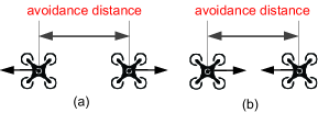
Figure 2: Intuitive interpretation for the definition of filtered position.

In this section, the motion of each multicopter is transformed into a single integrator form to simplify the controller design and analysis. As shown in Figure 2, although the position distances are the same, namely a marginal avoidance distance, the case in Figure 2(b) needs to carry out avoidance urgently by considering the velocity. However, the case in Figure 2(a) does not need to be considered to perform collision avoidance in fact. With such an intuition, a filtered position is defined as follows:

$$\boldsymbol{\xi}_{i}\triangleq\mathbf{p}_{i}+\frac{1}{l_{i}}\mathbf{v}_{i}.$$ (5)

Then

$$\boldsymbol{\dot{\xi}}_{i} =\mathbf{\dot{p}}_{i}+\frac{1}{l_{i}}\mathbf{\dot{v}}_{i}=\mathbf{v}_{\text{c},i}$$ (6)

where $i=1,2,\cdots,M$. Define the position error and the filtered position error between two multicopters as

$$\mathbf{\tilde{p}}{}_{\text{m,}ij} \triangleq\mathbf{p}_{i}-\mathbf{p}_{j}$$

$$\boldsymbol{\tilde{\xi}}{}_{\text{m,}ij} \triangleq\boldsymbol{\xi}_{i}-\boldsymbol{\xi}{}_{j}.$$

Proposition 1 [9] indicates that the position error is large enough as long as the filter position error is also large enough, which is shown as follows:

$$\left\|\mathbf{\tilde{p}}{}_{\text{m,}ij}\left(t\right)\right\|\geq\left\|\boldsymbol{\tilde{\xi}}{}_{\text{m,}ij}\left(t\right)\right\|-\max_{i}\frac{v_{\text{m},i}}{l_{i}}.$$ (7)

II-A3 Safety Radius Model

Three types of areas used for control for the $i$th multicopter, namely safety area $\mathcal{S}_{i}$, avoidance area $\mathcal{A}_{i}$, and detection area $\mathcal{D}_{i}$, are defined, as shown in Figure 3. The safety area $\mathcal{S}_{i}$ (to avoid a conflict) and avoidance area $\mathcal{A}_{i}$ (to start avoidance control) of the $i$th multicopter are circles (spheres in 3-dimensional case) both centered in its filtered position $\boldsymbol{\xi}_{i}$ with the safety radius $r_{\text{s}}$ and the avoidance area $r_{\text{a}}$, respectively. In addition, the detection area $\mathcal{D}_{i}$ only depends on the detection range of the used devices (by cameras, radars, 4G/5G mobile, or Vehicle to Vehicle (V2V) communication), which is centered in its position $\mathbf{p}_{i}$ with the detection radius $r_{\text{d}}$. The specific design principles of the safety radius are investigated in [27].

Remark 1. Intuitively, the basic design principle of safety radius is guided in (7). For two multicopters satisfying the model (1), the error between $\left\|\boldsymbol{\tilde{\xi}}{}_{\text{m,}ij}\left(t\right)\right\|$ and $\left\|\mathbf{\tilde{p}}{}_{\text{m,}ij}\left(t\right)\right\|$ has the upper bound $\max_{i}\frac{v_{\text{m},i}}{l_{i}}$. The condition for obtaining this upper bound is that two multicopters move on the same line and in opposite directions with maximum speed. To guarantee safety in this extreme case, the safety radius should be at least larger than the physical radius with $\max_{i}\frac{v_{\text{m},i}}{2l_{i}}$ for each multicopter. This indicates that the larger safety radius should be designed for the multicopter with higher speed or lower maneuverability if its physical radius is fixed.

Remark 2. It should be pointed out that the 2-dimensional case is just for simplicity of description, while similar analysis can also be extended to the 3-dimensional case. Specifically, the model (1) can add the z-axis kinematic function for each multicopter

$$\dot{p}_{\text{z}} =v_{\text{z}}$$

$$\dot{v}_{\text{z}} =-l_{\text{z}}\left(v_{\text{z}}-v_{\text{c,z}}\right)$$ (8)

where $p_{\text{z}},v_{\text{z}},v_{\text{c,z}}\in\mathbb{R}$ and $l_{\text{z}}>0$ are the z-axis position, velocity, velocity command and control gain of this multicopter, respectively. Note that the z-axis control gain $l_{\text{z}}$ is different from the horizontal control gain for multicopters in general. Further, the safety radius model can also be extended to the 3-dimensional case, while the safety area, avoidance area and detection area of a multicopter can be modeled as a sphere, a cylinder, or an ellipsoid rather than a circle. As for the stability analysis under the 3-dimensional case, similar proof can be given.

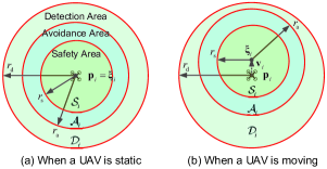
Figure 3: Safety area, avoidance area and detection area of a multcopter [9].

II-B Problem Formulation

The following assumptions are further needed. The position error and the filtered position error between the $i$th multicopter and its destination line $\mathcal{L}_{i}$ is defined as

$$\mathbf{\tilde{p}}{}_{\text{l,}i} \triangleq\mathbf{A}_{\text{l,}i}\left(\mathbf{p}_{i}-\mathbf{p}_{\text{l,}i}\right)$$

$$\boldsymbol{\tilde{\xi}}{}_{\text{l,}i} \triangleq\mathbf{A}_{\text{l,}i}\left(\boldsymbol{\xi}_{i}-\mathbf{p}_{\text{l,}i}\right)$$

where $\mathbf{A}_{\text{l,}i}=\mathbf{n}_{i}\mathbf{n}_{i}^{\text{T}}$ is the projection operator [28, p. 480]. By (6), the derivative of the filtered errors above are

$$\boldsymbol{\dot{\tilde{\xi}}}{}_{\text{l,}i} =\mathbf{A}_{\text{l,}i}\mathbf{v}_{\text{c},i}$$ (9)

$$\boldsymbol{\dot{\tilde{\xi}}}{}_{\text{m,}ij} =\mathbf{v}_{\text{c},i}-\mathbf{v}_{\text{c},j}$$ (10)

where $i\neq j$, $i,j=1,\cdots,M.$

Assumption 1. For each multicopter, the avoidance radius satisfies $r_{\text{a}}>r_{\text{s}}$, and the detection radius satisfies $r_{\text{d}}>r_{\text{s}}+r_{\text{a}}+2\underset{i}{\max}\frac{{v_{\text{m},i}}}{{l}_{i}}{.}$

Assumption 2. The multicopters’ initial positions satisfy

$$\left\|\boldsymbol{\tilde{\xi}}{}_{\text{m,}ij}\left(0\right)\right\|>2r_{\text{s}},i\neq j$$

where $i,j=1,2,\cdots,M.$

Assumption 3. Mathematically, a multicopter arrives at its destination line $\mathcal{L}_{i}$ if

$$\left\|\mathbf{v}_{i}\right\|<\epsilon_{\text{a}}\text{ and }\left\|\mathbf{\tilde{p}}{}_{\text{l,}i}\right\|\leq\epsilon_{\text{d}}.$$ (11)

where the sufficiently small $\epsilon_{\text{a}},\epsilon_{\text{d}}>0$ are given a priori. It implies that the multicopter arrives at the next region. Further, the multicopter will switch its destination line corresponding to its route, as shown in Figure 1.

Definition 1. Let the set $\mathcal{N}_{\text{m},i}$ be the collection of all mark numbers of other multicopters whose safety aeras enter into the avoidance area of the $i$th multicopter, namely

$$\mathcal{N}_{\text{m},i}=\left\{\left.j\right|\mathcal{S}_{j}\cap\mathcal{A}_{i}\neq\varnothing,j=1,\cdots,M,i\neq j\right\}.$$

According to Assumption 1, multicopters in $\mathcal{N}_{\text{m},i}$ can be detected by the ith multicopter. For example, if the safety areas of the $1$st, $2$nd multicopters enter into in the avoidance area of the $3$rd multicopter, then $\mathcal{N}_{\text{m},3}=\left\{1,2\right\}$.

Based on Assumptions 1-3, for cooperative multicopters, we have the free flight control problem stated in the following.

Objective. Let $\mathbf{p}_{i}$ and the line $\mathcal{L}_{i}$ be be the position and the destination line of the $i$th multicopter, respectively. Under Assumptions 1-3, design the velocity input $\mathbf{v}_{\text{c},i}$ for the $i$th multicopter with the information of its neighboring set $\mathcal{N}_{\text{m},i}$ to guarantee collision-avoidance and convergence to the destination line $\mathcal{L}_{i}$, i.e., $\left\|\boldsymbol{\tilde{\xi}}{}_{\text{l,}i}\right\|$ converges to zero and $\left\|\boldsymbol{\tilde{\xi}}{}_{\text{m,}ij}\left(t\right)\right\|>2r_{\text{s}}$ holds for $t>0$, $i=1,\cdots,M$.

Remark 3. According to Assumption 1, for the $i$th multicopter, any other multicopter entering into its avoidance area can be detected by the $i$th multicopter and will not conflict with the $i$th multicopter initially, $i=1,2,\cdots,M.$ Assumption 2 implies that any pair of two multicopters are not close too much initially. Assumption 3 is also reasonable in practice for air traffic, which is illustrated by the following example. Suppose that the $i$th and $j$th multicopters are located at two adjacent regions with the boundary line, while the task of each multicopter is to arrive at another region, as shown in Figure 4. To achieve this, the destination lines $\mathcal{L}_{i}$ and $\mathcal{L}_{j}$ can be chosen parallel to the boundary line of these two regions, and the distance between $\mathcal{L}_{i}$, $\mathcal{L}_{j}$ and the boundary line are both larger than $\epsilon_{\text{d}}$. Therefore, $\left\|\mathbf{\tilde{p}}{}_{\text{l,}i}\right\|\leq\epsilon_{\text{d}}$ implies that the $i$th multicopter has arrived at the $j$th region and the same for another multicopter.

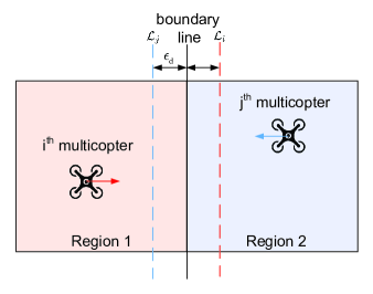
Figure 4: The intuitive explanation for Assumption 3. To achieve the next region, the destination line for each multicopter can be chosen parallel to the boundary line of two regions.

III Free Flight Control Problem for Multiple Cooperative Multicopters

The idea of the proposed method is similar to that of the APF method. In this method, the airspace is formulated as an APF. For a given multicopter, only is the corresponding destination line assigned attractive potential, while other multicopters are assigned repulsive potentials. A multicopter in the field will be attracted to the destination line, while being repelled by other multicopters.

III-A Preliminaries

In the following, two designed smooth functions $\sigma\left(\cdot\right)$ and $s\left(\cdot\right)$ are used for the following Lyapunov-like function design, which are defined as

$$\sigma\left(x,d_{1},d_{2}\right)=\left\{\begin{array}[]{c}1\\ Ax^{3}+Bx^{2}+Cx+D\\ 0\end{array}\right.\begin{array}[]{c}\text{if}\\ \text{if}\\ \text{if}\end{array}\begin{array}[]{c}x\leq d_{1}\\ d_{1}\leq x\leq d_{2}\\ d_{2}\leq x\end{array}$$ (12)

with $A=-2\left/\left(d_{1}-d_{2}\right)^{3}\right.,$ $B=3\left(d_{1}+d_{2}\right)\left/\left(d_{1}-d_{2}\right)^{3}\right.,$ $C=-6d_{1}d_{2}\left/\left(d_{1}-d_{2}\right)^{3}\right.$ , $D=d_{2}^{2}\left(3d_{1}-d_{2}\right)\left/\left(d_{1}-d_{2}\right)^{3}\right.$ and

$$s\left(x,\epsilon_{\text{s}}\right)=\left\{\begin{array}[]{c}x\\ \left(1-\epsilon_{\text{s}}\right)+\sqrt{\epsilon_{\text{s}}^{2}-\left(x-x_{2}\right)^{2}}\\ 1\end{array}\right.\begin{array}[]{c}0\leq x\leq x_{1}\\ x_{1}\leq x\leq x_{2}\\ x_{2}\leq x\end{array}$$ (13)

with $x_{2}=1+\frac{1}{\tan 67.5^{\circ}}\epsilon_{\text{s}}$ and $x_{1}=x_{2}-\sin 45^{\circ}\epsilon_{\text{s}}.$ The definition and properties of these designed functions is analyzed in [9]. A new type of Lyapunov functions for vectors, called Line Integral Lyapunov Function, is designed as

$$V_{\text{l,i}}\left(\mathbf{y}\right)=\int_{C_{\mathbf{y}}}\text{sat}\left(\mathbf{x},a\right)^{\text{T}}\text{d}\mathbf{x}$$ (14)

where $a>0,$ $\mathbf{x}\in\mathbf{\mathbb{R}}^{n},$ $C_{\mathbf{y}}$ is a line from $\mathbf{0}$ to $\mathbf{y}\in\mathbb{R}{}^{n}\mathbf{.}$ In the following lemma, we will show its properties.

Lemma 1 [9]. Suppose that the line integral Lyapunov function $V_{\text{l,i}}$ is defined as (14). Then (i) $V_{\text{l,i}}\left(\mathbf{y}\right)>0$ if $\left\|\mathbf{y}\right\|\neq 0$; (ii) if $\left\|\mathbf{y}\right\|\rightarrow\infty,$ then $V_{\text{l,i}}\left(\mathbf{y}\right)\rightarrow\infty;$ (iii) if $V_{\text{l,i}}\left(\mathbf{y}\right)$ is bounded, then $\left\|\mathbf{y}\right\|$ is bounded.

III-B Lyapunov-Like Function Design and Analysis

Define a smooth curve $C_{\boldsymbol{\tilde{\xi}}{}_{\text{l,}i}}$ from $\mathbf{0}$ to $\boldsymbol{\tilde{\xi}}{}_{\text{l,}i}$. Then, the line integral of $\text{sat}\left(\boldsymbol{\tilde{\xi}}{}_{\text{l,}i},v_{\text{m},i}\right)$ along $C_{\boldsymbol{\tilde{\xi}}{}_{\text{l,}i}}$ is

$$V_{\text{l},i}\left(\boldsymbol{\tilde{\xi}}{}_{\text{l,}i}\right)=\int_{C_{\boldsymbol{\tilde{\xi}}{}_{\text{l,}i}}}\text{sat}\left(k_{1}\boldsymbol{\tilde{\xi}}{}_{\text{l,}i},v_{\text{m},i}\right)^{\text{T}}\text{d}\mathbf{x}$$ (15)

where $k_{1}>0,$ $i=1,2,\cdots,M$. Note that the reason of using closed form of line integral in (15) includes avoiding specifying the norm in the saturation function (2) and making the physical meaning more intuitive. From the definition and Lemma 1, $V_{\text{w},i}\geq 0.$ Furthermore, define a barrier function as

$$V_{\text{m},ij}\left(\left\|\boldsymbol{\tilde{\xi}}{}_{\text{m,}ij}\right\|\right)=\frac{k_{2}\sigma_{\text{m}}\left(\left\|\boldsymbol{\tilde{\xi}}{}_{\text{m,}ij}\right\|\right)}{\left(1+\epsilon\right)\left\|\boldsymbol{\tilde{\xi}}{}_{\text{m,}ij}\right\|-2r_{\text{s}}s\left(\frac{\left\|\boldsymbol{\tilde{\xi}}{}_{\text{m,}ij}\right\|}{2r_{\text{s}}},\epsilon_{\text{s}}\right)}$$ (16)

where $k_{2},\epsilon>0.$ Here $\sigma_{\text{m}}\left(x\right)\triangleq\sigma\left(x,2r_{\text{s}},r_{\text{a}}+r_{\text{s}}\right)$, where $\sigma\left(\cdot\right)$ is defined in (12). The function $V_{\text{m},ij}$ has the following properties: (i) $\partial V_{\text{m},ij}\left/\partial\left\|\boldsymbol{\tilde{\xi}}{{}_{\text{m,}ij}}\right\|\right.\leq 0$; (ii) $\left\|\boldsymbol{\tilde{\xi}}{{}_{\text{m,}ij}}\right\|\geq r_{\text{a}}+r_{\text{s}}$ is a sufficient and necessary condition for $V_{\text{m},ij}=0$; (iii) if $0<\left\|\boldsymbol{\tilde{\xi}}{{}_{\text{m,}ij}}\right\|<2r_{\text{s}},$ namely $\mathcal{S}_{j}\cap\mathcal{S}_{i}\neq\varnothing$ (they may not collide in practice), then there exists a sufficiently small $\epsilon_{\text{s}}>0$ such that

$$V_{\text{m},ij}=\frac{k_{2}}{\epsilon\left\|\boldsymbol{\tilde{\xi}}{{}_{\text{m,}ij}}\right\|}=\frac{k_{2}}{2\epsilon r_{\text{s}}}.$$ (17)

The objective of the designed velocity command is to make $V_{\text{l},i}\left(\boldsymbol{\tilde{\xi}}{}_{\text{l,}i}\right)$ and $V_{\text{m},ij}\left(\left\|\boldsymbol{\tilde{\xi}}{}_{\text{m,}ij}\right\|\right)$ be zero or as small as possible. According to Lemma 1 and property (ii), this implies $\left\|\boldsymbol{\tilde{\xi}}{}_{\text{l,}i}\right\|\rightarrow 0$ and$\ \left\|\boldsymbol{\tilde{\xi}}{{}_{\text{m,}ij}}\right\|>r_{\text{a}}+r_{\text{s}}$, namely the $i$th multicopter will arrive at the destination line $\mathcal{L}_{i}$ and not conflict with the $j$th multicopter.

III-C Controller Design

The velocity command is designed as

$$\mathbf{v}_{\text{c},i}=-\text{sat}\left(\text{sat}\left(k_{1}\boldsymbol{\tilde{\xi}}{}_{\text{l,}i},v_{\text{m},i}\right)-\underset{j\in\mathcal{N}_{\text{m},i}}{\sum}b_{ij}\boldsymbol{\tilde{\xi}}{}_{\text{m,}ij},v_{\text{m},i}\right)$$ (18)

where $i=1,2,\cdots,M.$ Here $b_{ij}=0,$ $i,j=1,\cdots,M,$ $i\neq j$ if (11) holds; otherwise

$$b_{ij}=-\frac{\partial V_{\text{m},ij}}{\partial\left\|\boldsymbol{\tilde{\xi}}{}_{\text{m,}ij}\right\|}\frac{1}{\left\|\boldsymbol{\tilde{\xi}}{}_{\text{m,}ij}\right\|}.$$ (19)

In (18), the parameters $r_{\text{a}},r_{\text{s}}$ appear in $\sigma_{\text{m}}\left(x\right)$ included in (16) and further (19), where Assumption 1 has to be satisfied.

Remark 4. The saturation the term $\text{sat}\left(k_{1}\boldsymbol{\tilde{\xi}}{}_{\text{l,}i},v_{\text{m},i}\right)$ in (18) is very necessary in practice. Without the saturation, the velocity command (18) becomes

$$\mathbf{v}_{\text{c},i}=\mathbf{-}\text{sat}\left(k_{1}\boldsymbol{\tilde{\xi}}{}_{\text{l,}i}-\underset{j\in\mathcal{N}_{\text{m},i}}{\sum}b_{ij}\boldsymbol{\tilde{\xi}}{}_{\text{m,}ij},{v_{\text{m},i}}\right).$$

In this case, if $\left\|\boldsymbol{\tilde{\xi}}{}_{\text{l,}i}\left(0\right)\right\|$ is very large, then the term $k_{1}\boldsymbol{\tilde{\xi}}{}_{\text{l,}i}$ will dominate until the multicopter is very close to another so that $b_{ij}\boldsymbol{\tilde{\xi}}{{}_{\text{m,}ij}}$ will dominate. At that time, the multicopter will start to change the velocity to avoid the conflict. In practice, it may be too late by taking various uncertainties into consideration. The use of the maximum speeds $v_{\text{m},i}$ in the term $\text{sat}\left(k_{1}\boldsymbol{\tilde{\xi}}{}_{\text{l,}i},v_{\text{m},i}\right)$ of the velocity command (18) will avoid such a danger.

Remark 5. It should be noted that, in most literature, if their distance is less than a safety distance, then their control schemes either do not work or even push the agent towards the center of the safety area rather than leaving the safety area. Theses have been explained in Introduction. The proposed controller can also handle the case such as $\left\|\boldsymbol{\tilde{\xi}}{{}_{\text{m,}ij_{i}}}\right\|<2r_{\text{s}}$, which may still happen in practice due to unpredictable uncertainties. However, this may not imply that the $i$th multicopter have collided with the $j_{i}$th multicopter physically, because the redundancy is always considered when we design the safety radius $r_{\text{s}}$, i.e., $r_{\text{s}}$ is larger than the physical radius of the multicopter. In this case, there exists a sufficiently small $\epsilon_{\text{s}}>0$ such that

$$b_{ij_{i}}=b_{j_{i}i}=\frac{k_{2}}{\epsilon}\frac{1}{\left\|\boldsymbol{\tilde{\xi}}{}_{\text{m,}ij_{i}}\right\|^{3}}.$$

Since $\epsilon$ is chosen to be sufficiently small, the terms $b_{ij_{i}}\boldsymbol{\tilde{\xi}}{}_{\text{m,}ij_{i}}$ and $b_{j_{i}i}\boldsymbol{\tilde{\xi}}{}_{\text{m,}j_{i}i}$ will dominate so that the velocity commands $\mathbf{v}_{\text{c},i}$ and $\mathbf{v}_{\text{c},j_{i}}$ become

$$\mathbf{v}_{\text{c},i} =\text{sat}\left(\frac{k_{2}}{\epsilon}\frac{1}{\left\|\boldsymbol{\tilde{\xi}}{}_{\text{m,}ij_{i}}\right\|^{2}}\frac{\boldsymbol{\tilde{\xi}}{}_{\text{m,}ij_{i}}}{\left\|\boldsymbol{\tilde{\xi}}{}_{\text{m,}ij_{i}}\right\|},v_{\text{m},i}\right)$$

$$\mathbf{v}_{\text{c},j_{i}} =\text{sat}\left(\frac{k_{2}}{\epsilon}\frac{1}{\left\|\boldsymbol{\tilde{\xi}}{}_{\text{m,}j_{i}i}\right\|^{2}}\frac{\boldsymbol{\tilde{\xi}}{}_{\text{m,}j_{i}i}}{\left\|\boldsymbol{\tilde{\xi}}{}_{\text{m,}j_{i}i}\right\|},v_{\text{m},j_{i}}\right).$$

This implies that, by recalling (10), $\left\|\boldsymbol{\tilde{\xi}}{}_{\text{m,}ij_{i}}\right\|$ will be increased fast so that the $i$th multicopter and the $j_{i}$th multicopter can keep away from each other immediately. This implies that the proposed controller still works when Assumption 2 is violated, which indicates the robustness of the proposed controller and makes it more feasible in practice.

III-D Stability Analysis

In order to investigate the convergence to the destination line and the multicopter avoidance behaviour, a function is defined as follows

$$V_{1}=\underset{i=1}{\overset{M}{\sum}}\left(V_{\text{l},i}+\frac{{1}}{2}\underset{j=1,j\neq i}{\overset{M}{\sum}}V_{\text{m},ij}\right)$$ (20)

where $V_{\text{l},i}$ is defined in (15) and $V_{\text{m},ij}$ is defined in (16). According to Thomas’ Calculus [29, p. 911], one has

$$V_{1}=\underset{i=1}{\overset{M}{\sum}}\left(\int\nolimits_{0}^{t}\text{sat}\left(k_{1}\boldsymbol{\tilde{\xi}}{}_{\text{l,}i},v_{\text{m},i}\right)^{\text{T}}\boldsymbol{\dot{\tilde{\xi}}}{}_{\text{l,}i}\text{d}\tau+\frac{1}{2}\underset{j=1,j\neq i}{\overset{M}{\sum}}V_{\text{m},ij}\right).$$

The derivative of $V_{1}$ along the solution to (9) and (10) is

$$\dot{V}_{1} =\underset{i=1}{\overset{M}{\sum}}\left(\text{sat}\left(k_{1}\boldsymbol{\tilde{\xi}}{}_{\text{l,}i},v_{\text{m},i}\right)-\underset{j=1,j\neq i}{\overset{M}{\sum}}b_{ij}\boldsymbol{\tilde{\xi}}{}_{\text{m,}ij}\right)^{\text{T}}\mathbf{v}_{\text{c},i}$$

where the property $b_{ij}=b_{ji}$ defined in (19) is used. If $j\notin\mathcal{N}_{\text{m},i},$ one has $\mathcal{A}_{j}\cap\mathcal{S}_{i}=\varnothing.$ Then $b_{ij}=0$ according to the property (ii) of $V_{\text{m},ij}$. Consequently,

$$\underset{j\in\mathcal{N}_{\text{m},i}}{\sum}b_{ij}\boldsymbol{\tilde{\xi}}{}_{\text{m,}ij}=\underset{j=1,j\neq i}{\overset{M}{\sum}}b_{ij}\boldsymbol{\tilde{\xi}}{}_{\text{m,}ij}.$$

By using the velocity input (18), $\dot{V}_{1}$ becomes

$$\dot{V}_{1} =-\underset{i=1}{\overset{M}{\sum}}\left(\text{sat}\left(k_{1}\boldsymbol{\tilde{\xi}}{}_{\text{l,}i},v_{\text{m},i}\right)-\underset{j\in\mathcal{N}_{\text{m},i}}{\sum}b_{ij}\boldsymbol{\tilde{\xi}}{}_{\text{m,}ij}\right)$$

$$\cdot\text{sat}\left(\text{sat}\left(k_{1}\boldsymbol{\tilde{\xi}}{}_{\text{l,}i},v_{\text{m},i}\right)-\underset{j\in\mathcal{N}_{\text{m},i}}{\sum}b_{ij}\boldsymbol{\tilde{\xi}}{}_{\text{m,}ij},v_{\text{m},i}\right)$$

$$\leq 0.$$

Further, the main result is stated.

Theorem 1. Under Assumptions 1-3, suppose the velocity command is designed as (18) for model (1). Then there exist positive parameters $k_{1},k_{2},\epsilon,\epsilon_{\text{s}}>0$ in the proposed controller such that $\lim_{t\rightarrow\infty}\left\|\mathbf{\tilde{p}}_{\text{l,}i}\left(t\right)\right\|<\epsilon_{\text{d}}$ and $\left\|\boldsymbol{\tilde{\xi}}{}_{\text{m,}ij}\left(t\right)\right\|>2r_{\text{s}}$, $t\in\left[0,\infty\right)$ for almost $\mathbf{\tilde{p}}_{\text{l,}i}(0)$, $i\neq j,$ $i,j=1,2,\cdots,M$.

Proof. Due to limited space, similar to Lemma 2 [9], we can prove that these multicopters are able to avoid conflict with each other, namely $\left\|\boldsymbol{\tilde{\xi}}{}_{\text{m,}ij}\left(t\right)\right\|>2r_{\text{s}}$, $i\neq j,$ $i,j=1,2,\cdots,M.$ In the following, the reason why each multicopter is able to arrive at the destination $\mathcal{L}_{i}$ is given. The invariant set theorem [30, p. 69] is used to do the analysis.

• First, we will study the property of function $V_{1}$. Let $\Omega=\left\{\left.\boldsymbol{\xi}_{1},\cdots\boldsymbol{\xi}_{M}\right|V_{1}\left(\boldsymbol{\xi}_{1},\cdots\boldsymbol{\xi}_{M}\right)\leq l\right\},$ $l>0.$ According to Lemma 2, $V_{\text{m},ij}>0.$ Therefore, $V_{1}\left(\boldsymbol{\xi}_{1},\cdots\boldsymbol{\xi}_{M}\right)\leq l$ implies $\underset{i=1}{\overset{M}{\sum}}V_{\text{l},i}\leq l.$ Furthermore, according to Lemma 1(iii), $\Omega$ is bounded. When $\left\|\left[\begin{array}[]{ccc}\boldsymbol{\xi}_{1}&\cdots&\boldsymbol{\xi}_{M}\end{array}\right]\right\|\rightarrow\infty,$ then $\underset{i=1}{\overset{M}{\sum}}V_{\text{l},i}\rightarrow\infty$ according to Lemma 1(ii), namely $V_{1}\rightarrow\infty.$

• Secondly, we will find the largest invariant set. Then show all multicopters can arrive at their corresponding destination lines. Now, recalling the property (4), $\dot{V}_{1}$$=0$ if and only if

  $$\text{sat}\left(k_{1}\boldsymbol{\tilde{\xi}}{}_{\text{l,}i},v_{\text{m},i}\right)-\underset{j\in\mathcal{N}_{\text{m},i}}{\sum}b_{ij}\boldsymbol{\tilde{\xi}}{}_{\text{m,}ij}=\mathbf{0}$$ (21)

  for $i=1,2,\cdots,M.$ Then $\mathbf{v}_{\text{c},i}=\mathbf{0}$ according to (18). Consequently, the equation (1) only holds if $\mathbf{v}_{i}=\mathbf{0}$ for $i=1,2,\cdots,M$. Obviously, the equilibrium points are stable if $\left\|\boldsymbol{\tilde{\xi}}{}_{\text{l,}i}\right\|=0$ and $\left\|\boldsymbol{\tilde{\xi}}{}_{\text{m,}ij}\right\|>2r_{\text{a}}$, $i,j=1,2,\cdots,M.$ The objective here is to prove that the other equilibrium points $\left\|\mathbf{\tilde{p}}_{\text{l,}i}\right\|\geq\epsilon_{\text{d}}$ are unstable. According to (3), define

  $$\kappa_{i}=\kappa_{v_{\text{m},i}}\left(k_{1}\boldsymbol{\tilde{\xi}}{}_{\text{l,}i}\right)=\left\{\begin{array}[]{c}1,\\ \frac{v_{\text{m},i}}{k_{1}\left\|\boldsymbol{\tilde{\xi}}_{\text{l,}i}\right\|},\end{array}\begin{array}[]{c}\left\|\boldsymbol{\tilde{\xi}}_{\text{l,}i}\right\|\leq\frac{v_{\text{m},i}}{k_{1}}\\ \left\|\boldsymbol{\tilde{\xi}}_{\text{l,}i}\right\|>\frac{v_{\text{m},i}}{k_{1}}\end{array}\right..$$ (22)

  Note that the parameter $k_{1}$ can be sufficiently large such that the relation $k_{1}>\frac{v_{\text{m},i}}{\epsilon_{\text{d}}}$ holds, which implies that the input $k_{1}\mathbf{\tilde{p}}{}_{\text{l,}i}$ can keep saturated according to Assumption 3, and only the case $\left\|\boldsymbol{\tilde{\xi}}_{\text{l,}i}\right\|>\frac{v_{\text{m},i}}{k_{1}}$ in (22) should be considered. Then the equation (21) can be further written as

  $$\text{ sat}\left(k_{1}\boldsymbol{\tilde{\xi}}{}_{\text{l,}i},v_{\text{m},i}\right)-\underset{j\in\mathcal{N}_{\text{m},i}}{\sum}b_{ij}\boldsymbol{\tilde{\xi}}{}_{\text{m,}ij}$$

  $$= v_{\text{m},i}\frac{\boldsymbol{\tilde{\xi}}{}_{\text{l,}i}}{\left\|\boldsymbol{\tilde{\xi}}_{\text{l,}i}\right\|}-\underset{j\in\mathcal{N}_{\text{m},i}}{\sum}b_{ij}\boldsymbol{\tilde{\xi}}{}_{\text{m,}ij}=\mathbf{0}.$$

  Define

  $$\mathbf{v}_{\text{c},i}^{*}\triangleq v_{\text{m},i}\frac{\boldsymbol{\tilde{\xi}}{}_{\text{l,}i}}{\left\|\boldsymbol{\tilde{\xi}}_{\text{l,}i}\right\|}-\underset{j=1,j\neq i}{\overset{\bar{M}}{{\displaystyle\sum}}}b_{ij}\boldsymbol{\tilde{\xi}}{}_{\text{m,}ij}.$$ (23)

  For the ${\bar{M}}$ multicopters, substituting (18) into (6) results in

  $$\left[\begin{array}[]{c}\boldsymbol{\dot{\xi}}_{1}\\ \mathbf{\vdots}\\ \boldsymbol{\dot{\xi}}_{\bar{M}}\end{array}\right] =\mathbf{f}\left(\boldsymbol{\xi}_{1},\cdots,\boldsymbol{\xi}_{\bar{M}}\right)=-\left[\begin{array}[]{c}\kappa_{v_{\text{m},1}}^{\prime}\mathbf{v}_{\text{c},1}^{*}\\ \mathbf{\vdots}\\ \kappa_{v_{\text{m},\bar{M}}}^{\prime}\mathbf{v}_{\text{c},\bar{M}}^{*}\end{array}\right]$$ (30)

  where $\underset{j\in\mathcal{N}_{\text{m},i}}{\sum}b_{ij}\boldsymbol{\tilde{\xi}}_{\text{m},ij}=\underset{j=1,j\neq i}{\overset{\bar{M}}{{\displaystyle\sum}}}b_{ij}\boldsymbol{\tilde{\xi}}{}_{\text{m,}ij}$ is used and $\kappa_{v_{\text{m},i}}^{\prime}$ is defined as

  $$\kappa_{v_{\text{m},i}}^{\prime} =\left\{\begin{array}[]{cc}1,&\left\|\mathbf{v}_{\text{c},i}^{*}\right\|\leq v_{\text{m},i}\\ \frac{v_{\text{m},i}}{\left\|\mathbf{v}_{\text{c},i}^{*}\right\|}\text{,}&\left\|\mathbf{v}_{\text{c},i}^{*}\right\|>v_{\text{m},i}\end{array}\right..$$ (33)

  Note that $\left.\mathbf{v}_{\text{c},i}^{*}\right|_{\boldsymbol{\xi}_{i}=\mathbf{p}_{i}^{\ast}}=0$ holds at the equilibrium point $\boldsymbol{\xi}_{i}=\mathbf{p}_{i}^{\ast}$, then $\left.\kappa_{v_{\text{m},i}}^{\prime}\right|_{\boldsymbol{\xi}_{i}=\mathbf{p}_{i}^{\ast}}=1$ holds. Then we can get the derivative of $\mathbf{f}\left(\boldsymbol{\xi}_{1},\boldsymbol{\xi}_{2},\cdots,\boldsymbol{\xi}_{\bar{M}}\right)$ with respect to $\left[\boldsymbol{\xi}_{1},\boldsymbol{\xi}_{2}\cdots,\boldsymbol{\xi}_{\bar{M}}\right]$ is

$$\left.\frac{\partial\mathbf{f}\left(\boldsymbol{\xi}_{1},\boldsymbol{\xi}_{2},\cdots,\boldsymbol{\xi}_{\bar{M}}\right)}{\partial\left(\boldsymbol{\xi}_{1},\boldsymbol{\xi}_{2}\cdots,\boldsymbol{\xi}_{\bar{M}}\right)}\right|_{\boldsymbol{\xi}_{i}=\mathbf{p}_{i}^{\ast}} = \left.\left(\Lambda_{1}+\Lambda_{2}\right)\right|_{\boldsymbol{\xi}_{i}=\mathbf{p}_{i}^{\ast}}$$

where the matrice $\mathbf{\Lambda}_{1},\Lambda_{2}$ are defined in the following

$$\mathbf{\Lambda}_{1} =\left[\begin{array}[]{cccc}b_{1}&-b_{12}&\cdots&-b_{1\bar{M}}\\ -b_{21}&b_{2}&\cdots&-b_{2\bar{M}}\\ \vdots&\vdots&\ddots&\cdots\\ -b_{\bar{M}1}&-b_{\bar{M}2}&\cdots&b_{\bar{M}}\end{array}\right]\otimes\mathbf{I}_{2}$$

$$\mathbf{\Lambda}_{2} =\left[\begin{array}[]{ccc}\underset{j=2}{\overset{{\bar{M}}}{{\displaystyle\sum}}}\boldsymbol{\tilde{\xi}}{}_{\text{m,}1j}\frac{\partial b_{1j}}{\partial\boldsymbol{\xi}_{1}}&\cdots&-\boldsymbol{\tilde{\xi}}{}_{\text{m,}1\bar{M}}\frac{\partial b_{1\bar{M}}}{\partial\boldsymbol{\xi}_{\bar{M}}}\\ \vdots&\ddots&\vdots\\ -\frac{\partial b_{{\bar{M}}1}}{\partial\boldsymbol{\xi}_{1}}\boldsymbol{\tilde{\xi}}{}_{\text{m,}\bar{M}1}\frac{\partial b_{{\bar{M}}1}}{\partial\boldsymbol{\xi}_{1}}&\vdots&\underset{j=1}{\overset{\bar{M}-1}{{\displaystyle\sum}}}\boldsymbol{\tilde{\xi}}{}_{\text{m,}\bar{M}j}\frac{\partial b_{\bar{M}j}}{\partial\boldsymbol{\xi}_{\bar{M}}}\end{array}\right].$$

where $\otimes$ denotes Kronecker product, and the relationship

$$\frac{\partial\left(\frac{\boldsymbol{\tilde{\xi}}{}_{\text{l,}i}}{\left\|\boldsymbol{\tilde{\xi}}{}_{\text{l,}i}\right\|}\right)}{\partial\boldsymbol{\xi}_{i}}=\frac{\partial\mathbf{n}_{i}}{\partial\boldsymbol{\xi}_{i}}=\mathbf{0}$$

is utilized according to the definition of $\boldsymbol{\tilde{\xi}}{}_{\text{l,}i}$. Note that the equilibrium point $\boldsymbol{\xi}_{i}=\mathbf{p}_{i}^{\ast}$ is unstable if and only if the matrix $\left.\Lambda\right|_{\boldsymbol{\xi}_{i}=\mathbf{p}_{i}^{\ast}}$ has at least one positive eigenvalue. By the definition of $b_{ij}$ in (19), the equation $\frac{\partial b_{ij}}{\partial\boldsymbol{\xi}_{j}}\boldsymbol{\tilde{\xi}}{{}_{\text{m,}ij}}=\frac{\partial b_{ji}}{\partial\boldsymbol{\xi}_{i}}\boldsymbol{\tilde{\xi}}{{}_{\text{m,}ji}}$ holds. Further, since $b_{ij}=b_{ji}$, the matrice $\Lambda_{1}$ and $\Lambda_{2}$ are both symmetric. Note that $\Lambda_{1}$ has the form of Laplacian matrix of a directed graph since $b_{ij}>0$ holds, so it is a positive semidefinite matrix according to Lemma 1 [31]. Further, define a column vector $\boldsymbol{\alpha}=\left[\begin{array}[]{ccc}\left(\mathbf{R}\boldsymbol{\xi}_{1}\right)^{\text{T}}&\cdots&\left(\mathbf{R}\boldsymbol{\xi}_{\bar{M}}\right)^{\text{T}}\end{array}\right]^{\text{T}}$, where $\mathbf{R}=\left[\begin{array}[]{cc}0&1\\ -1&0\end{array}\right]$ is the rotation matrix. Note that $\boldsymbol{\alpha}^{\text{T}}\Lambda_{2}=\mathbf{0}$, which implies that $\boldsymbol{\alpha}$ is the eigenvector of $\Lambda_{2}$ corresponding to zero eigenvalue. Then we have

$$\boldsymbol{\alpha}^{\text{T}}\left.\left(\Lambda_{1}+\Lambda_{2}\right)\right|_{\boldsymbol{\xi}_{i}=\mathbf{p}_{i}^{\ast}}\boldsymbol{\alpha} =\boldsymbol{\alpha}^{\text{T}}\left.\Lambda_{1}\right|_{\boldsymbol{\xi}_{i}=\mathbf{p}_{i}^{\ast}}\boldsymbol{\alpha}$$

$$=\underset{i=1}{\overset{\bar{M}}{{\displaystyle\sum}}}\underset{j=1,j\neq i}{\overset{\bar{M}}{{\displaystyle\sum}}}b_{ij}\left\|\boldsymbol{\tilde{\xi}}{}_{\text{m,}ij}\right\|^{2}.$$

This implies that one eigenvalue of $\left.\left(\Lambda_{1}+\Lambda_{2}\right)\right|_{\boldsymbol{\xi}_{i}=\mathbf{p}_{i}^{\ast}}$ at least has a positive real part. Therefore, the equilibrium point $\boldsymbol{\xi}_{i}=\mathbf{p}_{i}^{\ast}$ is unstable, which is in fact a saddle point (an intuitive explanation can be found in [22, pp. 325-326]), $i=1,\cdots,\bar{M}$. For a saddle point, it is stable in a subspace but unstable in the other space. The measure of the stable subspace in the whole space equals $0$ or the stability probability is $0$. Therefore, the equilibrium point $\mathbf{p}_{i}^{\ast}$ is unstable with probability 1, i.e., any small deviation will drive the multicopter away from $\mathbf{p}_{i}^{\ast}$. Therefore, $\lim_{t\rightarrow\infty}\left\|\mathbf{\tilde{p}}_{\text{l,}i}\left(t\right)\right\|<\epsilon_{\text{d}},$ $t\in\left[0,\infty\right)$. This complete the proof. $\square$

Remark 6. In Theorem 1, the uncertainties of systems are ignored, which implies the system is autonomous. Therefore, the condition of the invariant set theorem is satisfied to do the analysis. However, this does not mean that our method is infeasible to the environment subject to uncertainties such as noise, communication delay, packet loss, etc. A method is proposed in [27] with a principle that separates the safety radius design and controller design. In other words, we can design the controller under the ideal conditions and consider all the uncertainties in the safety radius design process. The safety radius should be larger than the physical radius of multicopters; in other words, the margin of safety radius design should take uncertainties into consideration. This also explains why the case $\left\|\boldsymbol{\tilde{\xi}}{{}_{\text{m,}ij_{i}}}\right\|<2r_{\text{s}}$ may happen in practice if the safety radius is designed inappropriately or the uncertainties violate the assumption for the safety radius design, as stated in Remark 5.

IV Simulation and Experiments

Simulations and experiments are given in the following to show the effectiveness of the proposed method, where a video about simulations and experiments is available on https://youtu.be/NWysjgzBP6s.

IV-A Numerical Simulation

A scenario of a $250\text{m}\times 250\text{m}$ square region is considered. Each multicopter will enter the region from a random side of the square with the safety radius $r_{\text{s}}=10$m, the avoidance radius $r_{\text{a}}=15$m, the maximum speed $v_{\text{m}}=20\text{m/s}$, the control gain $l_{i}=5$, and the destination line opposite to it entered. To show the effectiveness of the proposed controller clearly, $M=420$ multicopters will enter the region with a dynamic inflow, which is shown in Figure 7. A multicopter will be randomly placed on a boundary line of the region it will enter, which implies that Assumption 2 may be violated and cause a conflict suddenly; however, the proposed controller still works. This is to simulate the situation a multicopter appears in another’s safety area accidently. The snapshots of the region are shown in Figure 6, while the route of each multicopter is plotted. By the proposed controller, each multicopter will keep the safe distance larger than $2r_{\text{s}}=20$m with other cooperative multicopters almost the whole process (except the case that a confliction suddenly happens as the reason explained above). Without loss of generality, the minimum distance $\underset{j\neq i,j=1,2,\cdots,M}{\min}\left\|\boldsymbol{\tilde{\xi}}{}_{\text{m,}ij}\right\|$ for $i=1,2,\cdots,40$ is shown in Figure 7(a). Note that the minimum distance for a multicopter may be less than $2r_{\text{s}}=20$m when it encounters another multicopter which just enters the region. To indicate that each multicopter finally converges to its destination line, the distance between the $i$th multicopter and its destination line $\left\|\boldsymbol{\tilde{\xi}}{}_{\text{l,}i}\right\|$ for $i=1,2,\cdots,40$ is shown in Figure 7(b). The result is consistent with the properties of the controller we proposed.

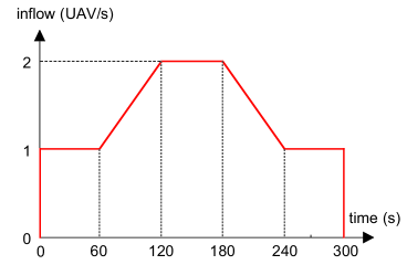
Figure 5: The dynamic inflow process of the $250\text{m}\times 250\text{m}$ square region.

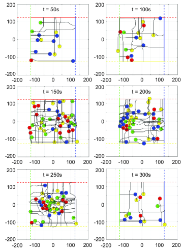
Figure 6: Simulation snapshots of the 250m$\times$250m square region. The color of each multicopter is consistent with its destination line.

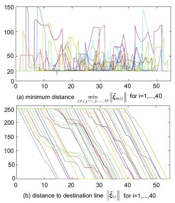
Figure 7: Minimum distance between the $i$th multicopter to others and distance between the $i$th multicopter to its destination line for $i=1,2,\cdots,40$.

IV-B Experiments

An indoor motion capture system called OptiTrack is installed in the lab, from which we can get the ground truth of the position, velocity and orientation of each multicopter. The laptop is running the proposed controller on MATLAB 2020a. The laptop obtains the position and velocity of each multicopter collected by optitrack through the local network, and further controls the multicopters through the UDP protocol. Based on the above conditions, a flight experiment is designed similarly to the simulation scenario, which contains eight multicopters located at four sides of a 2.5m$\times$2.5m square region initially. The multicopters used for the experiment is Tello multicopters released by DJI, where $r_{\text{s}}=0.2\text{m},$ $r_{\text{a}}=0.4\text{m},$ $v_{\text{m}}=0.15\text{m/s}$ are set. The destination line of each multicopter is directly opposite to its origin. The positions and the routes of multicopters during the whole flight experiment are shown in Figure 8. Finally, each multicopters can reach its destination line at about $t=63$s, keeping a safe distance from other multicopters without any conflict.

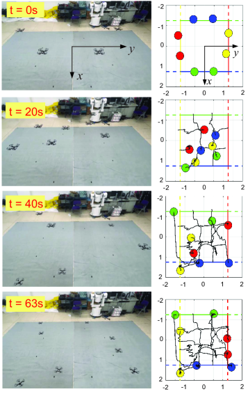
Figure 8: Multicopters’ positions at different time.

IV-C Discussion

The proposed control method can be easily extended to three-dimensional situations. Different from most formation control methods, the proposed method is more scalable and ensures that each agent completes its own independent mission. The agent uses only the navigation information of neighboring nodes to avoid potential collisions, so the topology can be arbitrary rather than limited to a set. Compared to the optimization based methods [32] and trajectory planning methods [33], the proposed method is convenient to implement in practical applications since it has low time complexity and avoids the computation-consuming iterative optimization procedure. Moreover, the designed controller has a larger domain than other Lyapunov-like function methods [19],[22], which improves safety under unpredictable uncertainties. Therefore, indoor robots and air traffic are both included in potential applications.

V Conclusions

The free flight control problem, which includes convergence to destination line and inter-agent conflict avoidance with each multicopter, is studied in this paper. Based on the velocity control model of multicopters with control saturation, practical distributed control is proposed for multiple multicopters to fly freely. Each multicopter has the same and simple control protocol. Lyapunov-like functions are designed with formal analysis and proofs showing that the free flight control problem can be solved. Besides the functional requirement, the safety requirement is also satisfied. By the proposed distributed control, a multicopter can keep away from another as soon as possible, once it enters into the safety area of another multicopter accidentally, which is very necessary to guarantee safety. Simulations and experiments are given to show the effectiveness of the proposed method from the functional and safety requirements.

Rao Fu received the B.S. degree in control science and engineering from Beihang University, Beijing, China, in 2017. He is working toward to the Ph.D. degree at the School of Automation Science and Electrical Engineering, Beihang University (formerly Beijing University of Aeronautics and Astronautics), Beijing, China. His main research interests include UAV traffic control and swarm.

Quan Quan received the B.S. and Ph.D. degrees in control science and engineering from Beihang University, Beijing, China, in 2004 and 2010, respectively. He has been an Associate Professor with Beihang University since 2013, where he is currently with the School of Automation Science and Electrical Engineering. His research interests include reliable flight control, vision-based navigation, repetitive learning control, and timedelay systems.

Mengxin Li is working toward to the M.S. degree at the School of Automation Science and Electrical Engineering, Beihang University (formerly Beijing University of Aeronautics and Astronautics), Beijing, China. Her main research interests include flight safety and control of multicopter.

Kai-Yuan Cai received the B.S., M.S., and Ph.D. degrees in control science and engineering from Beihang University, Beijing, China, in 1984, 1987, and 1991, respectively. He has been a Full Professor at Beihang University since 1995. He is a Cheung Kong Scholar (Chair Professor), jointly appointed by the Ministry of Education of China and the Li Ka Shing Foundation of Hong Kong in 1999. His main research interests include software testing, software reliability, reliable flight control, ADA (autonomous, dependable, and affordable) control, and software cybernetics.

References

- [1] M. Gharibi, R. Boutaba, S. L. Waslander, “Internet of drones,” IEEE Access, vol. 4, pp. 1148-1162, 2016.
- [2] S. Devasia and A. Lee, “A scalable low-cost-UAV traffic network (uNET),” Journal of Air Trasportation, vol. 24, pp. 74-83, 2016.
- [3] M. Xue, “Urban air mobility conflict resolution: centralized or decentralized?,” AIAA Aviation 2020 Forum, pp. 3192, 2020.
- [4] M. Xue and M. Do, “Scenario complexity for unmanned aircraft system traffic,” AIAA Aviation 2019 Forum, pp. 3513, 2019.
- [5] J. M. Hoekstra, R. C. J. Ruigrok, and R. N. H. W. van Gent, “Free flight in a crowded airspace,” Proceedings of the 3rd USA/Europe Air Traffic Management R&D Semi, Napoli, Italy, 2000, pp. 533–546.
- [6] J. M. Hoekstra, J. Ellerbroek, E. Sunil, J. Maas, “Geovectoring: reducing traffic complexity to increase the capacity of uav airspace,” International conference for research in air transportation, Barcelona, Spain. 2018.
- [7] AIRBUS, “Airbus skyways: the future of the parcel delivery in smart cities”[Online], Available:https://www.embention.com/project/ airbus-parcel-delivery/
- [8] Q. Quan, M. Li, R. Fu, “Sky highway design for dense traffic,” 16th IFAC Symposium on Control in Transportation Systems (CTS 2021), pp. 140-145, 2021.
- [9] Q. Quan, R. Fu, M. Li, D. Wei, Y. Gao, K-Y. Cai, “Practical control for practical distributed control for VTOL UAVs to pass a virtual tube,” IEEE Transactions on Intelligent Vehicles, doi: 10.1109/TIV.2021.3123110. (early access)
- [10] J. Qin, Q. Ma, Y. Shi, L. Wang, “Recent advances in consensus of multi-agent systems: a brief survey,” IEEE Transactions on Industrial Electronics, vol. 64, no. 6, pp. 4972-4983, 2017.
- [11] W. Ren and Y. Cao, “Overview of recent research in distributed multi-agent coordination,” in Distributed Coordination of Multi-agent Networks, London, U.K.:Springer-Verlag, pp. 23-41, 2011.
- [12] Y. Shi, J. Qin, H. Ahn, “Distributed coordination control and industrial applications,” IEEE Transactions on Industrial Electronics, vol. 64, no. 6, pp. 4967-4971, June 2017.
- [13] M. Hoy, A. S. Matvcev, A. V. Savkin, “Algorithms for collision-free navigation of mobile robots in complex cluttered environments: a survey,” Robotica, vol. 33, no. 03, pp. 463-497, 2015.
- [14] K. K. Oh, M.-C. Park, H. S. Ahn, “A survey of multi-agent formation control,” Automatica, vol. 53, pp. 424-440, 2015.
- [15] K. D. Do, “Formation control of mobile agents using local potential functions,” 2006 American Control Conference, pp. 2148-2153, 2006.
- [16] H. Rezaee and F. Abdollahi, “A decentralized cooperative control scheme with obstacle avoidance for a team of mobile robots,” IEEE Transactions on Industrial Electronics, vol. 61, no. 1, pp. 347-354, Jan. 2014.
- [17] S. Zhao, “Affine formation maneuver control of multi-agent systems,” IEEE Transactions on Automatic Control, vol. 63, no. 12, pp. 4140-4155, 2018.
- [18] D. V. Dimarogonas and K. J. Kyriakopoulos, “Distributed cooperative control and collision avoidance for multiple kinematic agents,” Decision and Control 2006 45th IEEE Conference, pp. 721-726, 2006.
- [19] D. Panagou, D. M. Stipanovic, P. G. Voulgaris, “Distributed coordination control for multi-robot networks using Lyapunov-like barrier functions,” IEEE Transactions on Automatic Control, vol. 61, no. 3, pp. 617-632, 2016.
- [20] E. G. Hernandez-Martinez, E. Aranda-Bricaire, F. Alkhateeb, E. A. Maghayreh, I. A. Doush, “Convergence and collision avoidance in formation control: A survey of the artificial potential functions approach,” in Multi-Agent Systems—Modeling Control Programming Simulations and Applications, Princeton, NJ:InTech, pp. 103-126, 2011.
- [21] L. Wang, A. D. Ames, M. Egerstedt, “Safety barrier certificates for collisions-free multirobot systems,” IEEE Transactions on Robotics, vol. 33, no. 3, pp. 661-674, Jun. 2017.
- [22] Q. Quan, Introduction to Multicopter Design and Control, Springer, 2017.
- [23] D. Yu, C. L. P. Chen and H. Xu, “Intelligent decision making and bionic movement control of self-organized swarm,” IEEE Transactions on Industrial Electronics, doi: 10.1109/TIE.2020.2998748. (to be published)
- [24] E. Rimon and D. Koditschek, “Exact robot navigation using artificial potential functions,” IEEE Transactions on Robotics and Automation, vol. 8, no. 5, pp. 501–518, 1992.
- [25] X. Xu, P. Tabuada, J. W. Grizzle, A. D. Ames, “Robustness of control barrier functions for safety critical control,” IFAC-PapersOnLine, vol. 48, no. 27, pp. 54-61, 2015.
- [26] Q. Quan, R. Fu, K-Y. Cai, “Practical control for multicopters to avoid non-cooperative moving obstacles,” IEEE Transactions on Intelligent Transportation Systems, doi: 10.1109/TITS.2021.3096558. (early access)
- [27] Q. Quan, R. Fu, K-Y. Cai, “How far two UAVs should be subject to communication uncertainties,” arXiv preprint arXiv:2110.09391v1, 2021.
- [28] N. Dunford and J. T. Schwartz, Linear Operators Part I: General Theory, Interscience, New York, 1958.
- [29] G. B. Thomas, M. D. Weir, J. R. Hass, F. R. Giordano, Thomas’ Calculus, Boston, MA, USA:Addison-Wesley, 2005.
- [30] J.-J. E. Slotine, W. Li, Applied Nonlinear Control, Englewood Cliffs, NJ:Prentice Hall, 1991.
- [31] W. Ren and R. W. Beard, “Consensus seeking in multiagent systems under dynamically changing interaction topologies,” IEEE Transactions on Automatic Control, vol. 50, no. 5, pp. 655–661, 2005.
- [32] B. T. Ingersoll, J. K. Ingersoll, P. DeFranco, A. Ning, “UAV path-planning using Bezier curves and a receding horizon approach,” AIAA Modeling and Simulation Technologies Conference. pp. 3675, 2016.
- [33] B. Xian, S. Wan , S. Yang, “An online trajectory planning approach for a quadrotor UAV with a slung payload,” IEEE Transactions on Industrial Electronics, vol. 67, no. 8, pp. 6669-6678, Aug. 2020.