Absorbing phase transition in a unidirectionally coupled layered network

Abstract

We study the contact process on layered networks in which each layer is unidirectionally coupled to the next layer. Each layer has elements sitting on i) Erdös-Réyni network, ii) a $d$-dimensional lattice. The layer at the top which is not connected to any layer. The top layer undergoes absorbing transition in the directed percolation class for the corresponding topology. The critical point for absorbing transition is the same for all layers. For Erdos-Reyni network order parameter $\rho(t)$ decays as $t^{-\delta_{l}}$ at the critical point for $l^{\prime}$th layer with $\delta_{l}\sim 2^{1-l}$. This can be explained with a hierarchy of differential equations in the mean-field approximation. The dynamic exponent $z$ is $0.5$ for all layers and the value of $\nu_{\parallel}$ tends to 2 for larger $l$. For a d-dimensional lattice, we observe stretched exponential decay of order parameter for all but top layer at the critical point.

Identification of underlying topological structure for complex systemsNakamura (2003) has led to the new branch of $`$network science’Börner et al. (2007). Several researchers have studied different properties of real-life networks and proposed models. Most popular among these models are scale-freeHein et al. (2006) and small-world networksNewman et al. (2011). The studies on networks helped to a better understanding for phenomena as diverse as the spreading of diseases in the population, information processing in gene circuits and biological pathways. It has also helped in understanding transport properties on several man-made system.

Another model which has attracted attention recently has been multiplex network. It models multiple levels of interaction in a given network. One example is a social media networkZhang et al. (2018); Kanawati (2015) where individuals are connected by twitter, facebook, whatsapp, etc. The same individual could be connected to different individuals in various layers and there is certain information flow in the layers. Another example is traffic networkTian et al. (2016) where people travel using various modes of travel such as tram, bus, etc. In spread of diseasesSanz et al. (2014); de Arruda et al. (2017), empirical studies on different strains of disease or different diseases have shown the necessity of modeling the underlying network as a multiplex network. In a multiplex network, the interaction between the nodes is described by a single layer network and the different layers of networks describe the different modes of interaction. Various properties such as properties of random walkGuo et al. (2016) on these networks, eigenvalueGomez et al. (2013) and eigenvector structure of these networks, spread of infection on such networks etc. have been investigated.

In this work, we study a simplified model of multilayer networks where all layers have the same type of connectivity within a given layer. Every agent is connected to the agent in the next layer in a unidirectional manner. We study the contact process on this network. For low infection probability $p$, the infection dies down and number of infected individuals goes to zero. For higher $p$, the fraction of infected individuals tends to a constant. Usually, this is an absorbing transition in the universality class of directed percolation. We study this model on the network mentioned above and find that the nature of decay of order parameter at the critical point changes from layer to layer. Interestingly, for a random network, we observe a power-law decay of order parameter with different exponents for different layers. On the other hand, for 1-d or 2-d basic networks, we find that the decay is well described by stretched exponential at the critical point for all but top layer.

First, we consider a multiplex network with $L$ layers each having $N$ agents. Each layer has Erdös-Réyni type random network, i.e. each site is coupled to $k$ randomly chosen sites in the same layer for top layer and same connectivity is repeated for all $L$ layers. Each site is connected to the previous layer unidirectionally. Each $m^{th}$ site in $j^{th}$ layer is connected to $m^{th}$ site in $j-1^{th}$ layer of the lattices in unidirectional way for $j>1$. The top layer ($j=1$) is not connected to layer. The representative picture of random network topology for only two layers and for $k=2$ is shown in Fig.1 (a). Apart from a random network, we have also considered cartesian lattice as a network for the top layer in later sections. Representative multiplex structure for 1-D network for 4 layers is shown in Fig.1 (b).

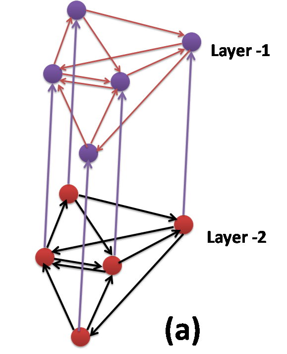
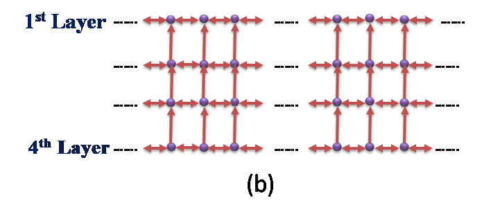
Figure 1: (a)Topological representation of random network system. (b)Topological representation of 1-D network system.

We have carried out extensive numerical simulations for contact process on above random multiplex network where the top layer is a random network with $k=4$. We define the contact process on this network as follows. We associate variable $x^{j}_{m}(t)$ to $m$’th site on $j$’th layer of this $NL$ dimensional multiplex where $L$ is a number of layers each of which has $N$ sites. Initially, we assign $x^{j}_{m}(0)=0$ or $x^{j}_{m}(0)=1$ with equal probability. We define $s^{j}_{m}(t)$ as sum of $x^{j}_{m}(t)$ which are connected to $x_{m}^{j}$. The evolution proceeds in a synchronous manner as $x^{j}_{m}(t+1)=1$ with probability $p$ if $s^{j}_{m}(t)\neq 0$ and 0 otherwise. In other words, each site becomes active with probability $p$ if any of the sites it is connected with is active. Being a contact process, this model shows the transition to an absorbing state. If all sites in the multiplex become inactive, they remain so forever. Furthermore, we observe another feature. Due to unidirectional connection between layers, if the entire top layer become inactive, it remains so forever because it is not connected to any other layer. Similarly, if all sites in the top two layers become inactive, they stay inactive regardless of the presence of active sites in the next layers. On the other hand, $j$th inactive layer can become active if there are active sites in any $l$th layer such that $l<j$. We expect the value of $p_{c}$ to be the same for the entire lattice as it is for the top layer. The reason is simple. Below $p_{c}$, the top layer will become inactive. Now immediate next layer is the top layer for all practical purposes and will become inactive and so on.

For a random network with $k$ neighbors, we expect the absorbing state for $kp<1$ in the mean-field limit. Thus we estimate $p_{c}=1/k$. For $k=4$, we numerically obtain $p_{c}=0.25000\pm 0.00015$ which is close to this approximation. It is expected that the dynamic phase transition for random connectivity will be in the same universality class as the mean-field class. For non-equilibrium phase transitions, this expectation is not always fulfilledGade and Sinha (2005); Mahajan et al. (2013).

The top layer is not connected to any layer and thus the critical point as well as the critical exponents for absorbing phase transition in the top layer must be in the same universality class as the absorbing phase transition for that connectivity. As mentioned above, this is also the critical point for the entire multiplex structure. However, we may question how the critical exponents (if any) change for layers below the top layer.

We study the 6-layers random network in which we study the absorbing phase transition using order parameter $O_{l}(t)$ which is a fraction of active sites in $l^{th}$ layer as a quantifier. We indeed observe power-law decay of order parameter at the critical point $p=p_{c}$ for all $l$. The order parameter goes like $1/t^{\delta_{l}}$ for each layer $p=p_{c}$. The power-law exponent value for the top layer is close to $\delta_{1}=1$. For layer below the top layer is $\delta_{2}=0.5$ and so on. The magnitude of the power-law exponent of a layer decreases as we go down the layers. The value of $\delta_{l}$ for $l^{th}$ layer is half the value for $(l-1)^{th}$ layer. Due to continuous infusion of infection from layers above, the inactivation rate becomes slower for larger $l$. This is shown in figure 2(a). An excellent power-law is obtained with $\delta_{l}=2^{1-l}$ for $l>1$ while for $l=1$, we obtain value $\delta_{1}=1$ which is equal to expected mean-field value 1. This behavior is confirmed by plotting $O_{l}(t)t^{\delta_{l}}$ as a function of time $t$ and independent fits (see fig. 2(b)). These values are confirmed within $1\%$. We note that $O_{l}(t)t^{\delta_{l}}$ is constant in time over a few decades. While the exponent in the top-layer is an expected exponent in mean-field class, other exponents are new.

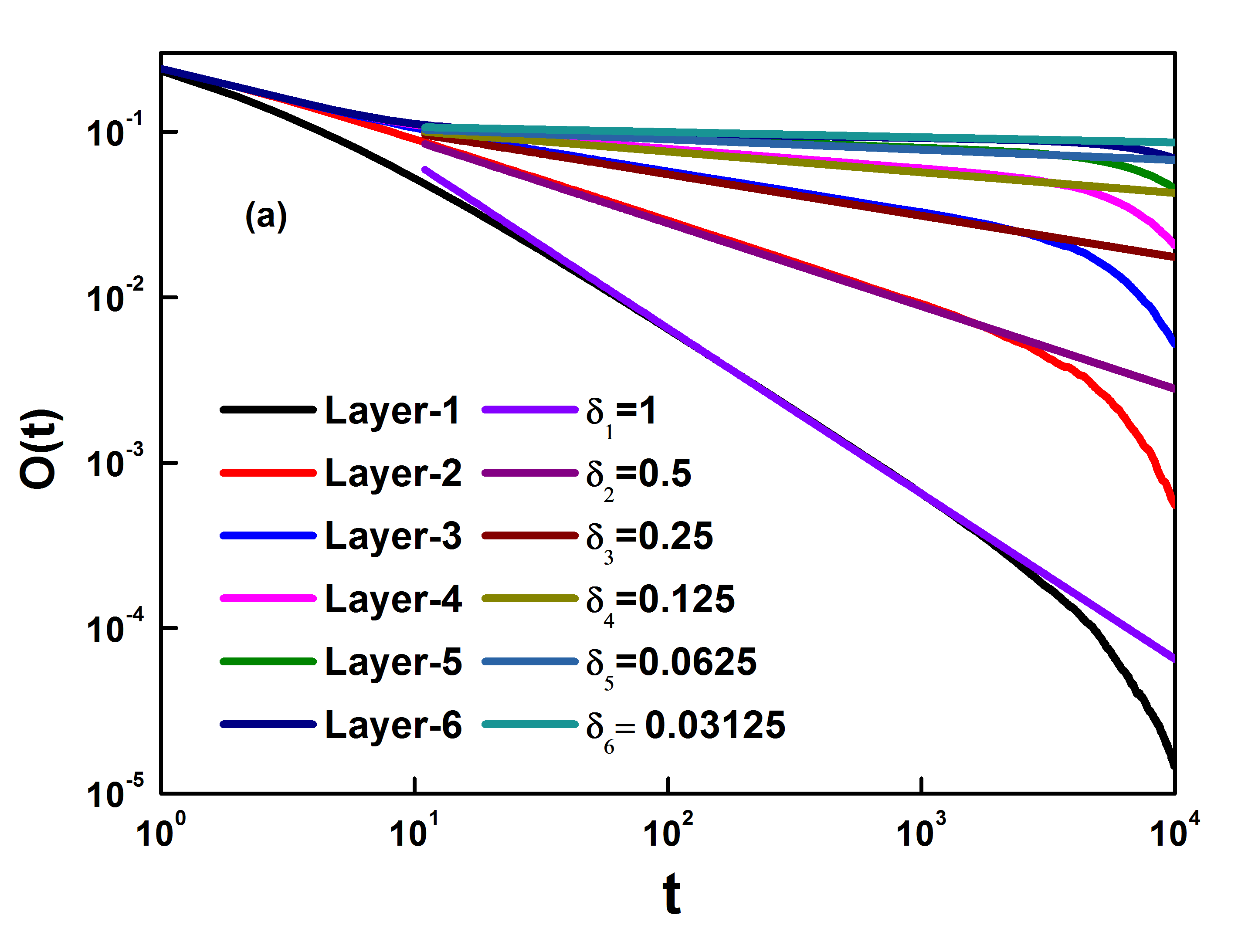
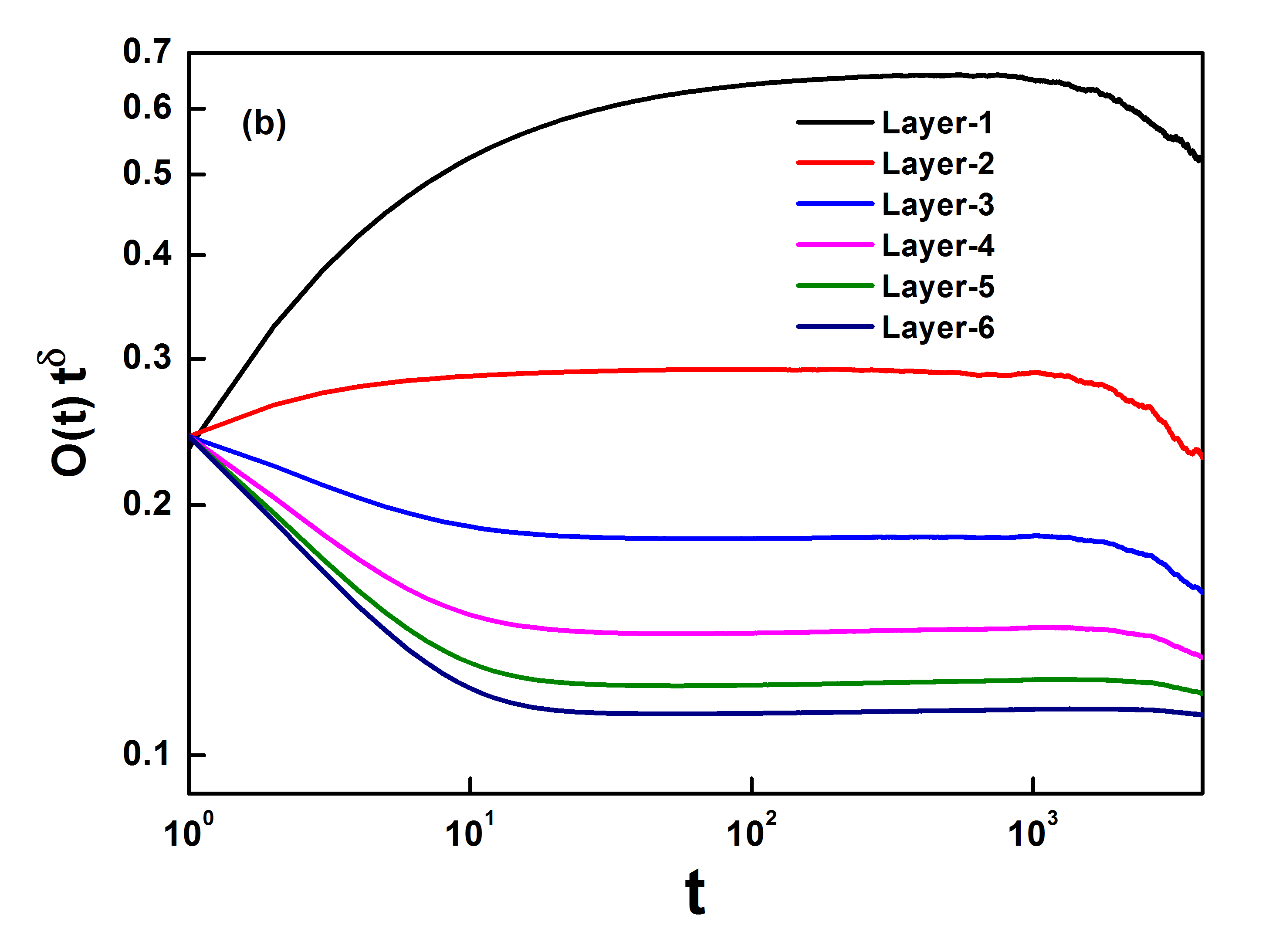
Figure 2: a) We plot order prameter $O_{l}(t)$ as function of time $t$ for various layers (from bottom to top) of random network at $p=p_{c}=0.25$. The lattice size is $N=8\times 10^{6}$. The decay exponent is given from $\delta_{l}=1-2^{-l}$ and the fit is shown as guide to eye. b) The quantity $O_{l}(t)t^{\delta_{l}}$ is plotted as a fuction of $t$ (from top to bottom). We observe that this quantity is a constant in time confirming $\delta_{l}$.

We study the finite-size scaling at the critical point for different layers. We simulate for $N=$ 100, 200, 400, 800, 1600, 3200, 6400, 12800, 25600, 51200. We have average over $2\times 10^{6}$ or more configurations for $N\leq 12800$ and over $2\times 10^{5}$ configurations for $N\geq 25600$. We obtain finite-size scaling for every layer in the network. The dynamical exponent value for all layers is the same and has the value $z=0.5$. The finite-size scaling for each layer is shown in figure 3.

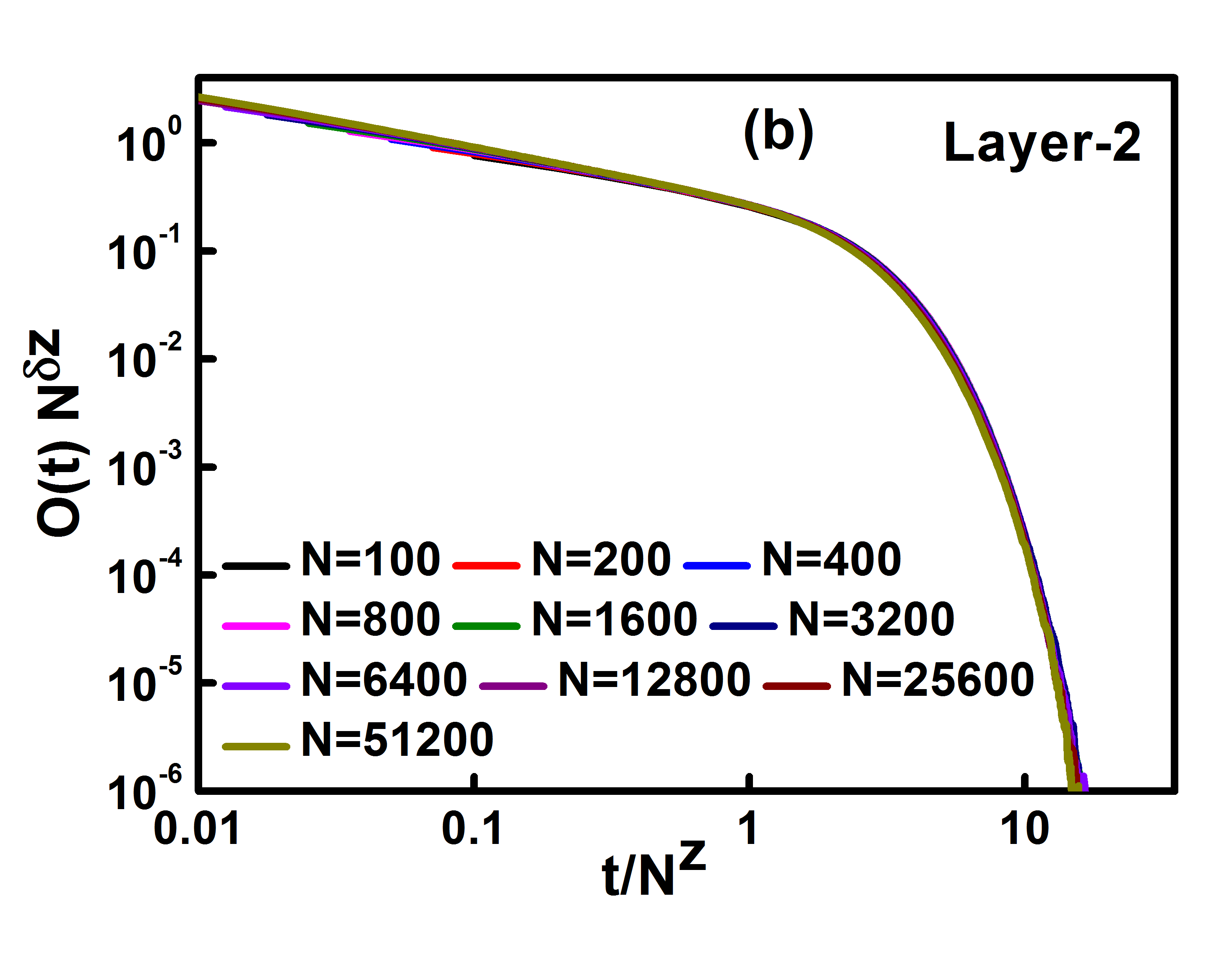
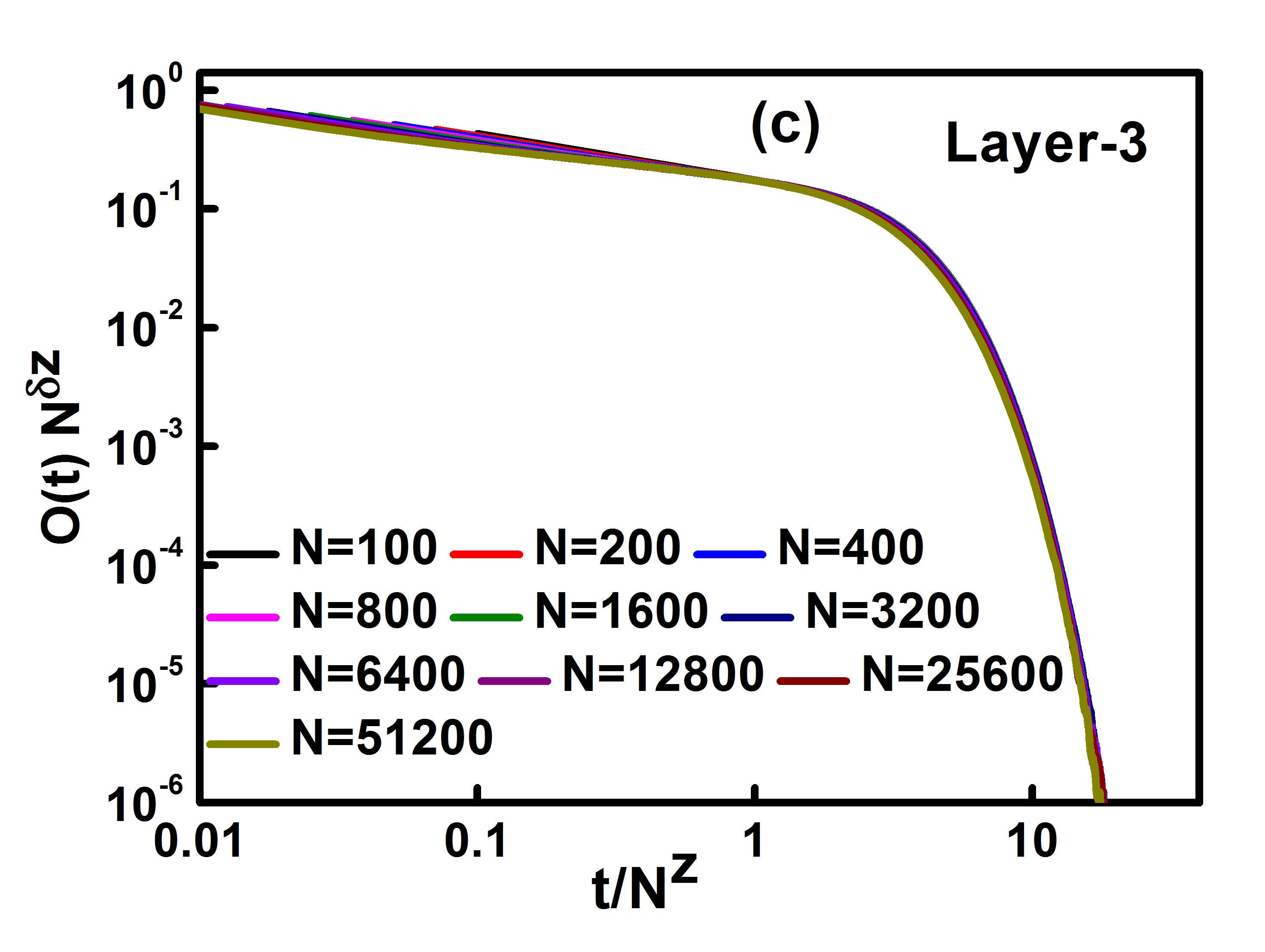
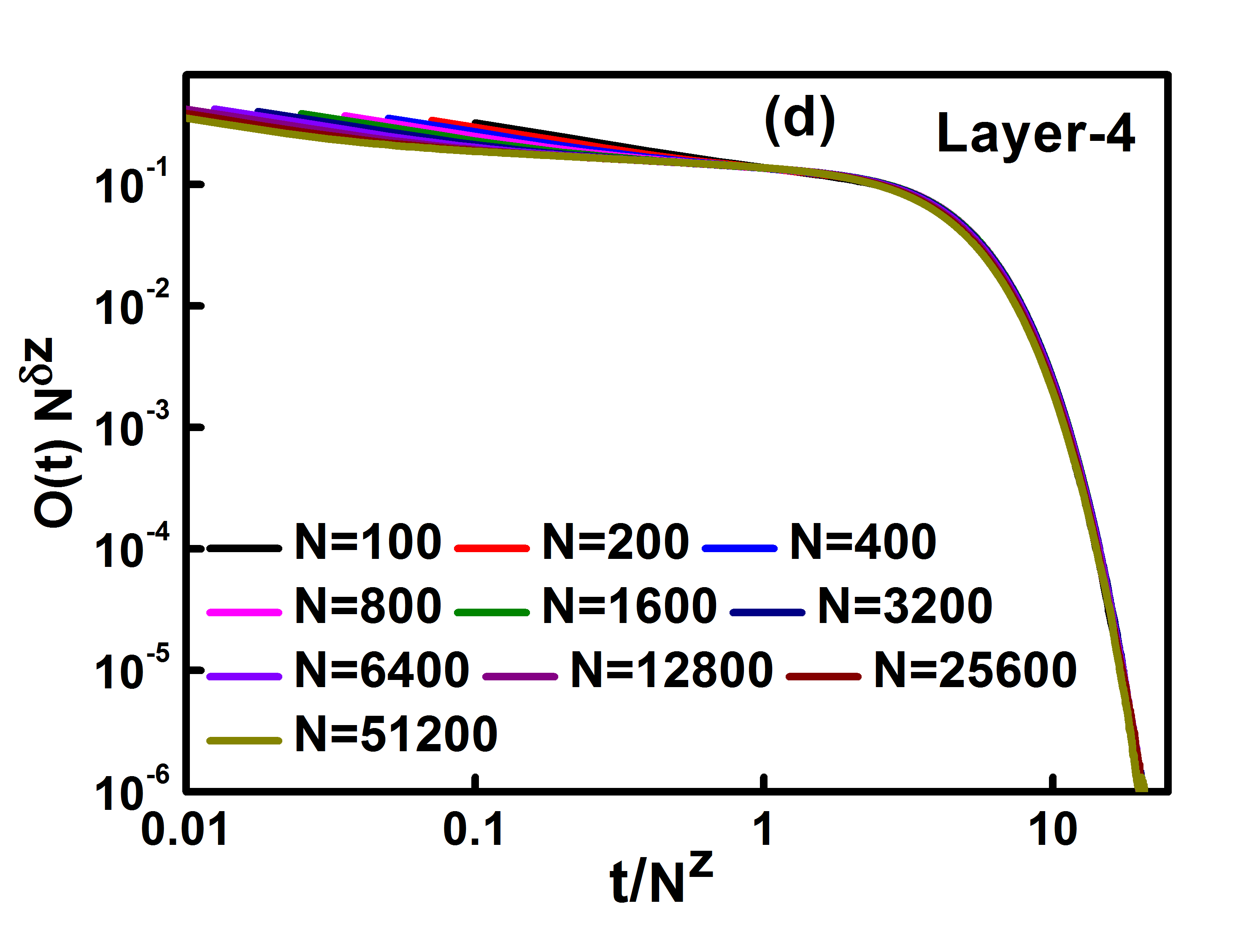
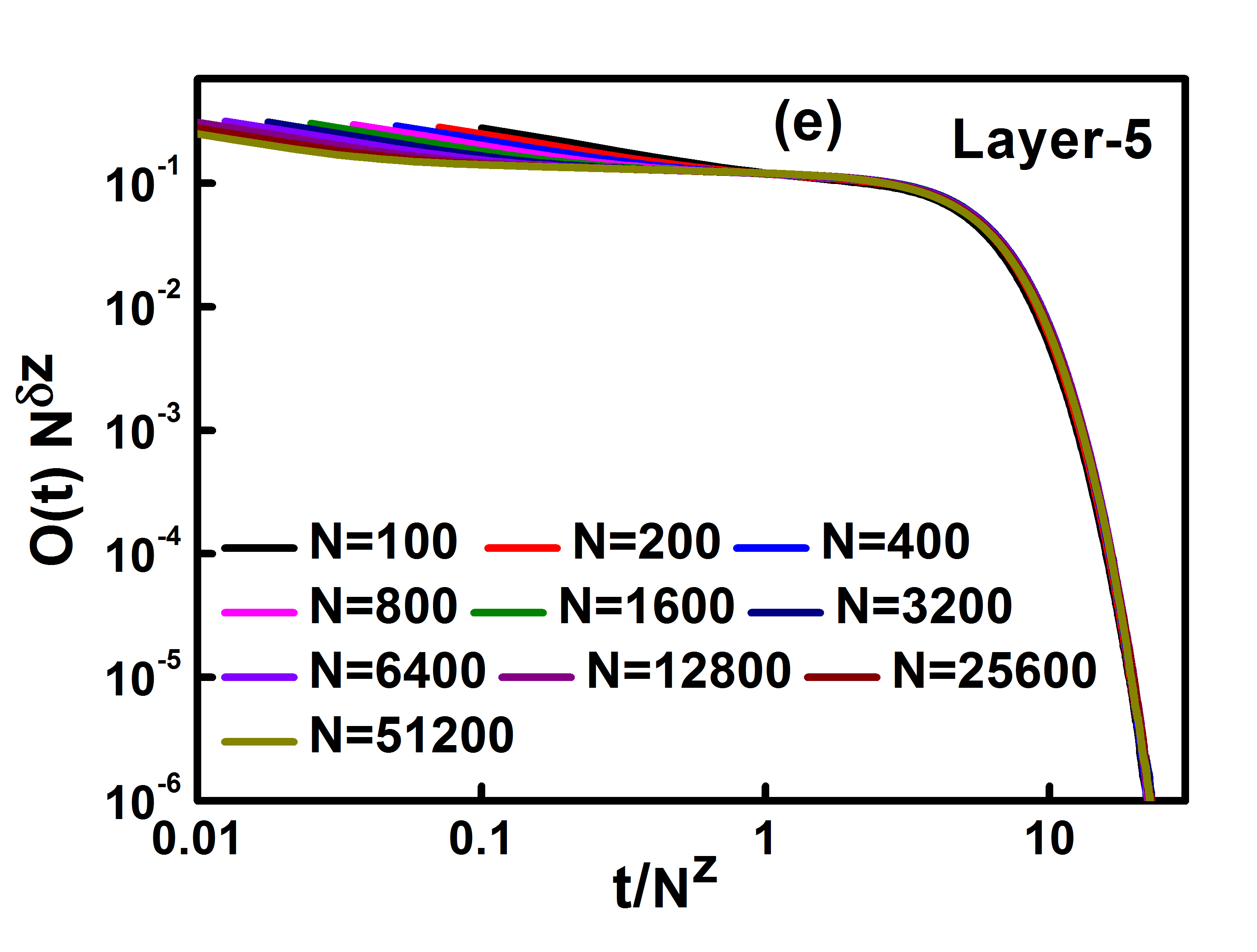
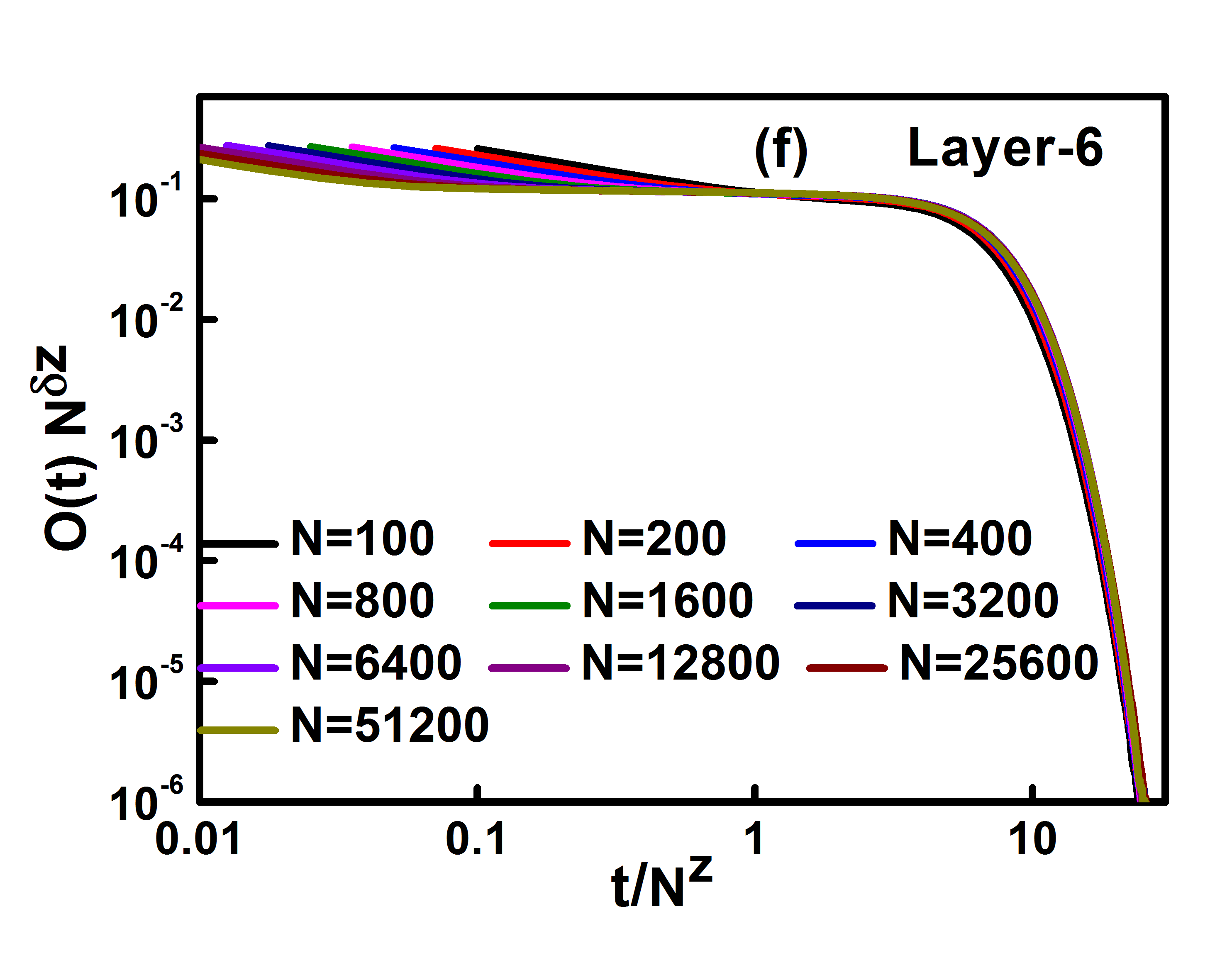
Figure 3: For random network, we carry out finite size scaling by plotting plot $O_{j}(t)N^{z\delta_{l}}$ as a function of $t/N^{z}$ for different system size $N$ at $p=p_{c}=0.25$ where $\delta_{l}=2^{1-l}$ and $\delta_{1}=1$. The value of dynamical exponent $z=0.5$ is same for all layers. a) Layer-1 b) Layer-2 c) Layer-3 d) Layer-4 e) Layer-5 f) Layer-6

We expect the asymptotic value of order parameter to scale as $O_{l}(\infty)\propto\Delta^{\beta_{l}}$ where $\Delta=|p-p_{c}|$ and $O_{l}(\infty)$ is the fraction of active sites in $l^{th}$ layer. We also note that $\beta_{l}=\nu_{\parallel,l}\delta_{l}$ We carry out simulations for $N=8\times 10^{6}$ and average over more than $80$ configurations (see fig.4). (We fit the function $O_{l}(\infty)\propto a\Delta^{b}$ using fit function in gnuplot and values of $b$ obtained from fiting is closely match with the exponent $\beta_{l}$ obtained using visual fit.) We find that $\nu_{\parallel,1}=\delta_{1}=1$ for first layer which are mean-field values. However for $l\neq 1$, $\nu_{\parallel,l}>1$ and $\beta_{l}\neq\delta_{l}$ for $l>1$. In fact $\nu_{\parallel,l}\rightarrow 2$ for higher layers.

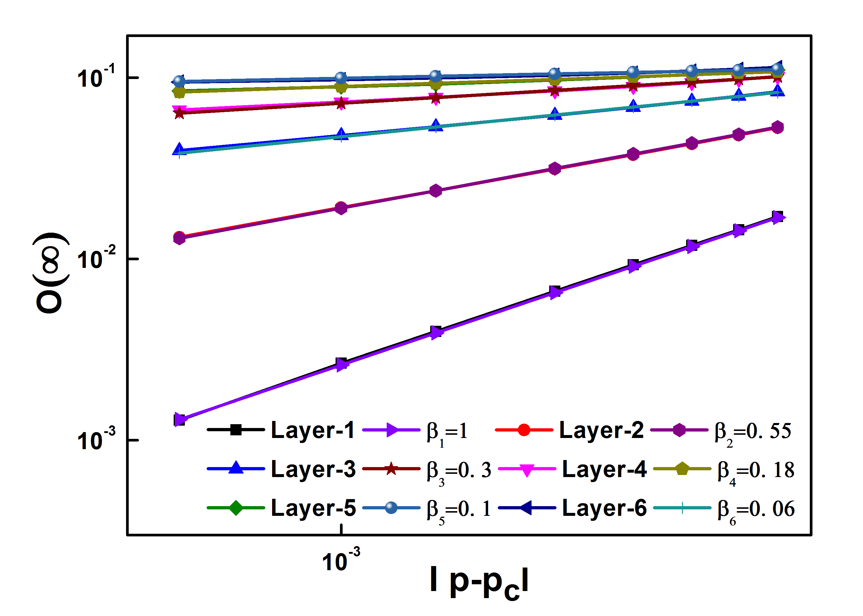
Figure 4: The $O_{l}(\infty)$ is plotted for various values of $\Delta$ ranging from $0.0005-0.0065$ for various layers (from bottom to top). The behavior can be appoximated as $O_{l}(\infty)\propto\Delta^{\beta_{l}}$ with $\beta_{l}=\nu_{\parallel,l}\delta_{l}$, and $\nu_{\parallel,1}=1$ $\nu_{\parallel,2}=1.1$ $\nu_{\parallel,3}=1.2$ $\nu_{\parallel,4}=1.44$ $\nu_{\parallel,5}=1.6$ $\nu_{\parallel,6}=1.92$.

To understand this behavior, we write mean-field equations for various layers. The mean field equation for directed percolateion is given by Eq. 3.6 in Henkel et al. (2008). $\partial_{t}\rho_{1}(t)=\tau\rho_{1}(t)-g\rho_{1}(t)^{2}$. for the critical point $\tau=0$, $\rho_{1}(t)={\frac{1}{c+gt}}$ where $c=(\rho_{1}(0))^{-1}$. Thus $\delta_{1}=1$. For $\tau>0$ $\rho_{1}(t)\sim{\frac{\tau}{g}}$ as $t\rightarrow\infty$ implying $\beta_{1}=1$ and hence $\nu_{\parallel}=1$ as expected in mean field limit. We heuristically write equations for different layers as

$$\partial_{t}\rho_{1}(t)=\tau\rho_{1}(t)-g\rho_{1}(t)^{2}$$

$$\partial_{t}\rho_{2}(t)=\tau\rho_{2}(t)-g\rho_{2}(t)^{2}+\rho_{1}(t)$$

$$\vdots$$

$$\partial_{t}\rho_{l}(t)=\tau\rho_{l}(t)-g\rho_{l}(t)^{2}+\rho_{l-1}(t)$$

$$\vdots$$

$$\partial_{t}\rho_{L}(t)=\tau\rho_{L}(t)-g\rho_{L}(t)^{2}+\rho_{L-1}(t)$$ (1)

We simulate these equations at the critical point $\tau=0$ using fourth-order Runge-Kutta method with $h=0.01$ with $\rho_{i}(0)=0.9$ for $1\leq i\leq L$. Asymptotically, we observe a power-law decay of order parameter as $\rho_{l}(t)\sim t^{\delta}_{l}$ with $\delta_{l}=2^{1-l}$. These plots are shown in Fig. 5. Thus the hierarchy of mean-field equations explains the order density decay exponent at $p=p_{c}$ very well.

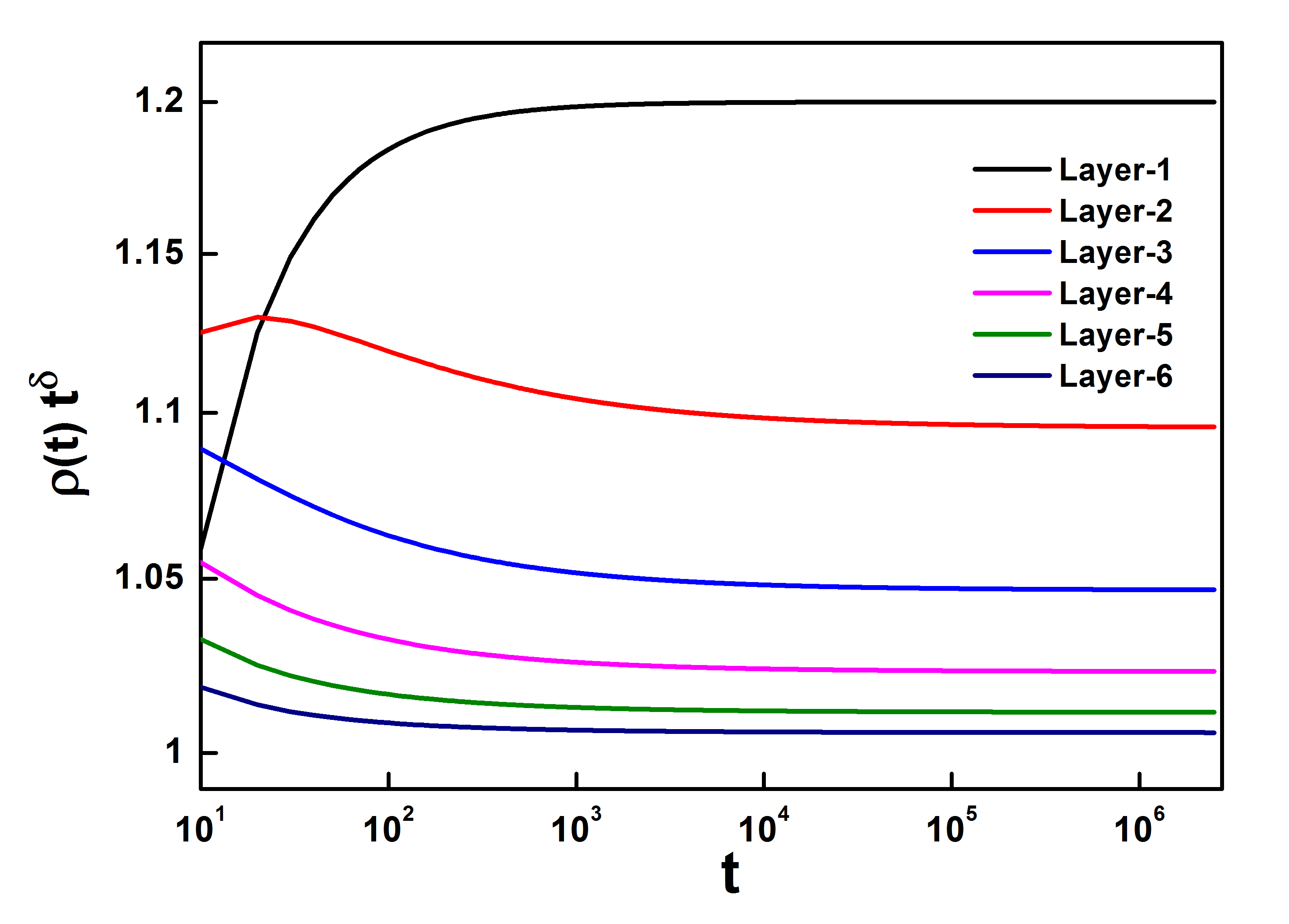
Figure 5: The $t^{\delta_{l}}\rho_{l}(t)$ is plotted as function of time $t$ for various layers (from top to bottom).

However for $\tau>0$, the behaviour does not match with random multiplex described above. In an analogous manner, we propose $\rho_{l}(\infty)\propto\tau^{\beta_{l}}$ and obtain $\beta_{l}=\delta_{l}$. Thus $\nu_{\parallel}=1$ for all layers which are expected for the mean-field system. This is not reproduced for random network multiplex. The reason may be long crossover times or the mean-field limit may be approached for very large values of $k$. We have noted above that it is not necessary that non-equilibrium systems on random networks show a transition in the mean-field class.

We also consider the case in which each layer has internal connections like a d-dimensional cartesian lattice. Let us consider the case of 1-d lattice and $L$ layers. We study the system for $L=4$. We carry out the simulations for $N=2\times 10^{5}$ and averaged over $220$ configuration. The critical point $p_{c}=0.70548515$ is knownHenkel et al. (2008) and is the same for all layers of network. As expected, there is clear power-law decay of order parameter with critical exponent $\delta=0.159$ for the first layer. (see fig.6) This behavior is expected. This absorbing phase transition is the same as in the DP class of 1-D lattice for the top layer.

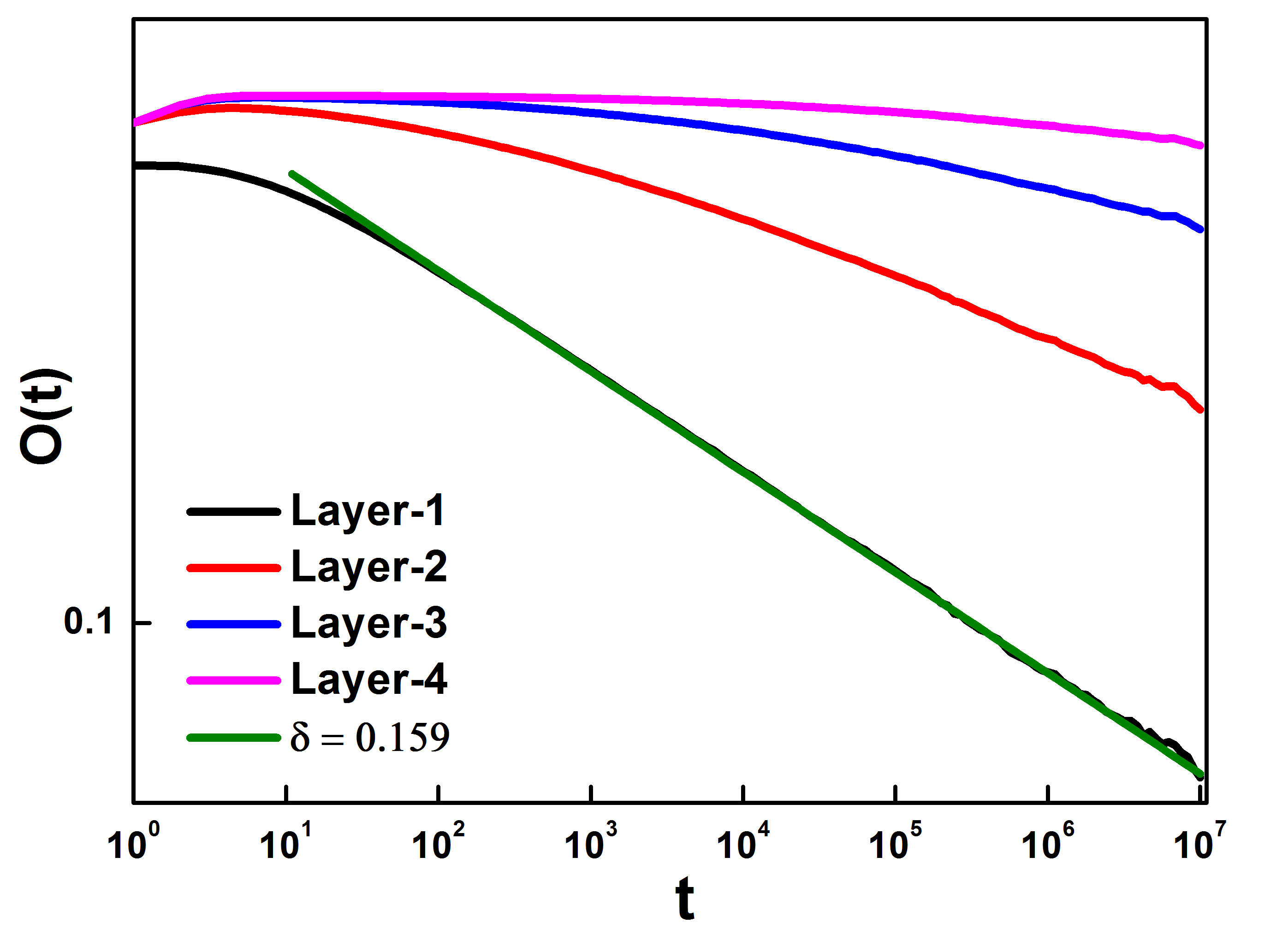
Figure 6: We plot $O_{l}(t)$ as function of time $t$ for 1-D network (from bottom to top) for $N=2\times 10^{5}$ and $p=P_{c}=0.70548515$. The order parameter decay exponent for top layer is $\delta=0.159$.

However, the decay of order parameter for layers below the top layer is not a power-law decay. It is better fitted by a stretched exponential. Except first layer, all other layers show a stretched exponential decay of order parameter as $\rho_{l}(t)\propto\exp(-B_{l}x^{c_{l}})$ and the value of $c_{l}$ increases with $l$ (see fig.7). The values of $C_{l}$ are $0.09,0.16$ and $0.24$ within $3\%$ for the second, third, and fourth layers. This behavior is confirmed by fitting using standard software such as OriginEdwards (2002) and using a fit function in Gnuplot which uses an implementation of the nonlinear least-squares(NLLS) Marquardt-Levenberg algorithmRanganathan (2004).

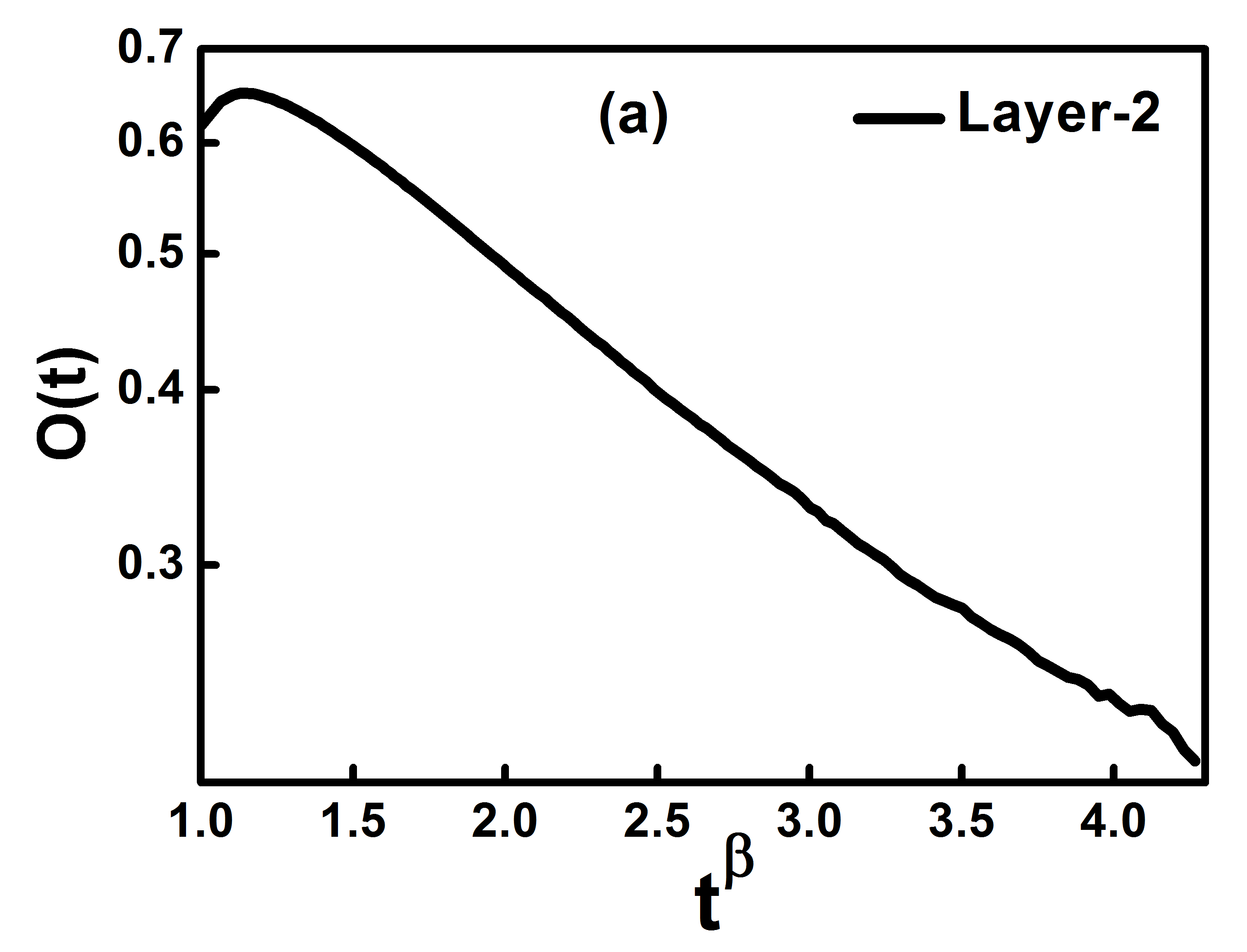
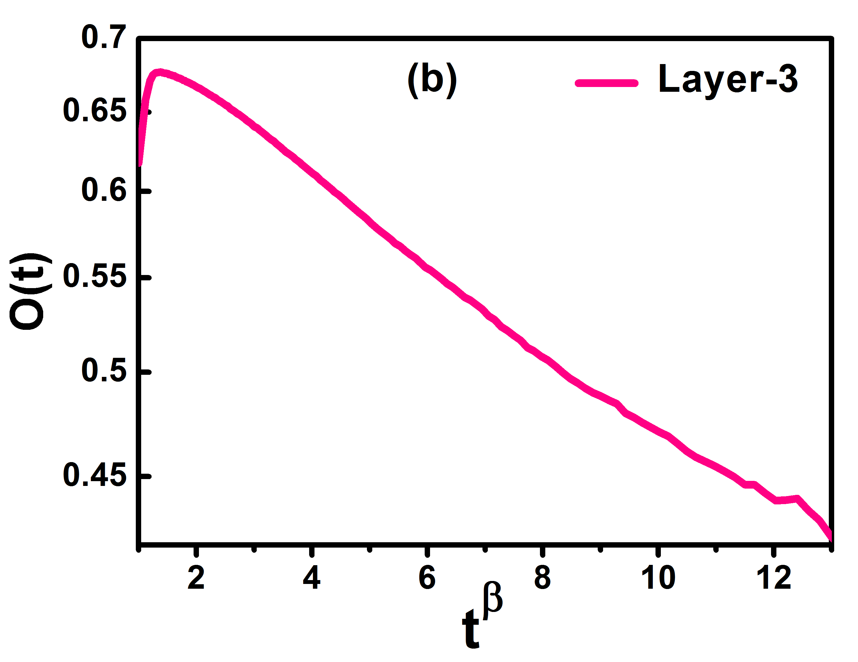
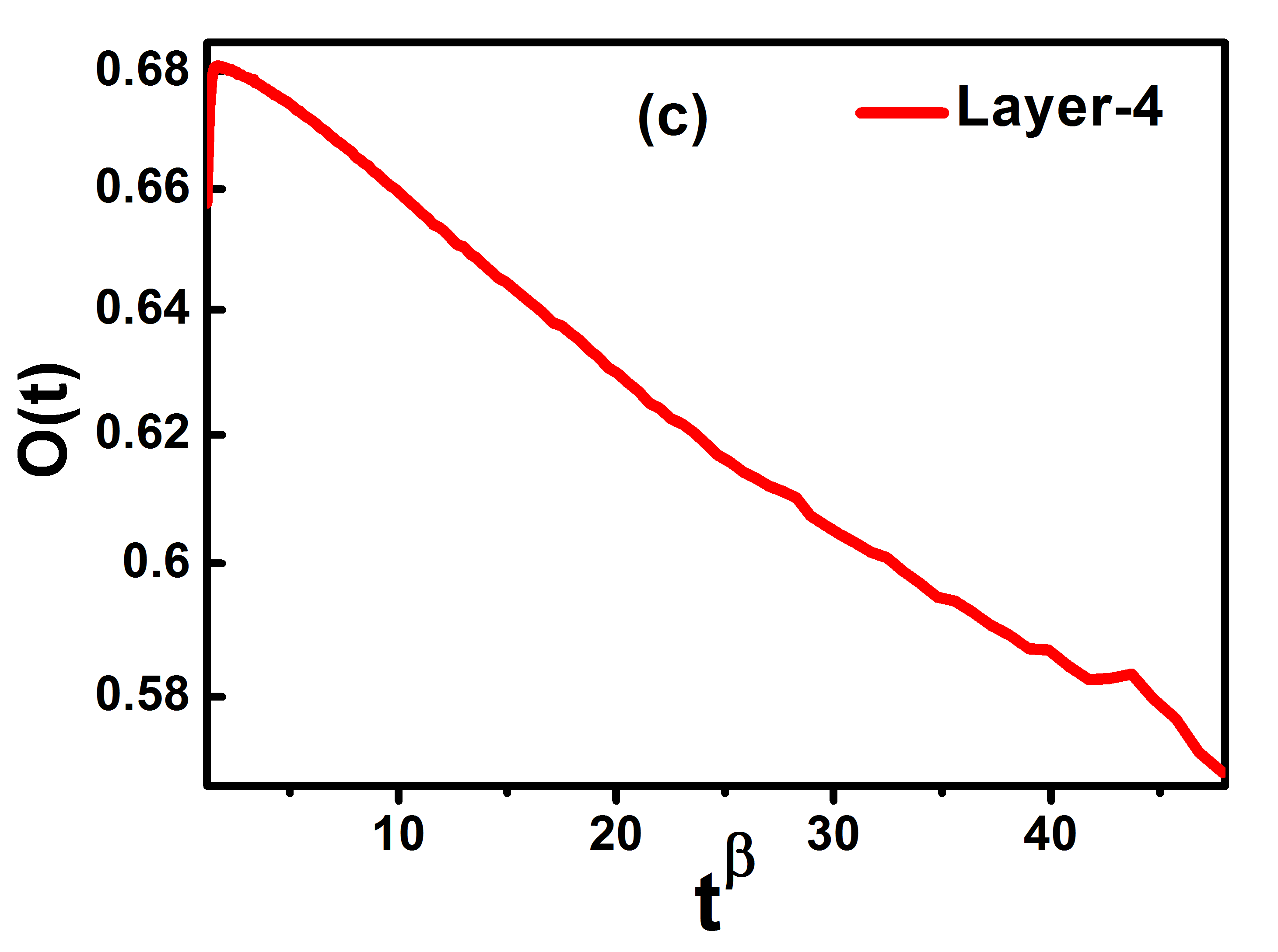
Figure 7: For 1D, we plot $O_{j}(t)$ vs. $t^{\beta}$ on semi-logarithmic scale for $j\neq 1$ at $p=p_{c}$. A clear straight line shows that decay is well described by stretched exponential. (a) j=2, $\beta=0.09$ (b) j=3, $\beta=0.16$ (c) j=4, $\beta=0.24$

We carry out similar investigations for the case where the network in a given layer is 2-d. We simulate $N\times N$ lattice in a given layer with $N=2.5\times 10^{3}$ at $p=p_{c}=0.34457$. We averaged over $85$ configuration and consider 4 layers. The order parameter show a power-law decay with exponent $\delta=0.45$ for the first layer as expected for DP class(see fig.8). However, others layers bend downwards on a log-log scale and decay is faster than power law. As in the case of 1-D, it is described by a clear stretched exponential decay. For 2D network the values of $C_{l}$ are $0.12,0.23$ and $0.41$ within $1\%$ for second, third, and fourth layers. The plots are shown in figure 9. For $l=4$ in 2-D, curvature indicates the the possible presence of strong nonlinear corrections to stretched exponential fit. We note that stretched exponential is a very poor fit $l\neq 1$ for random network.

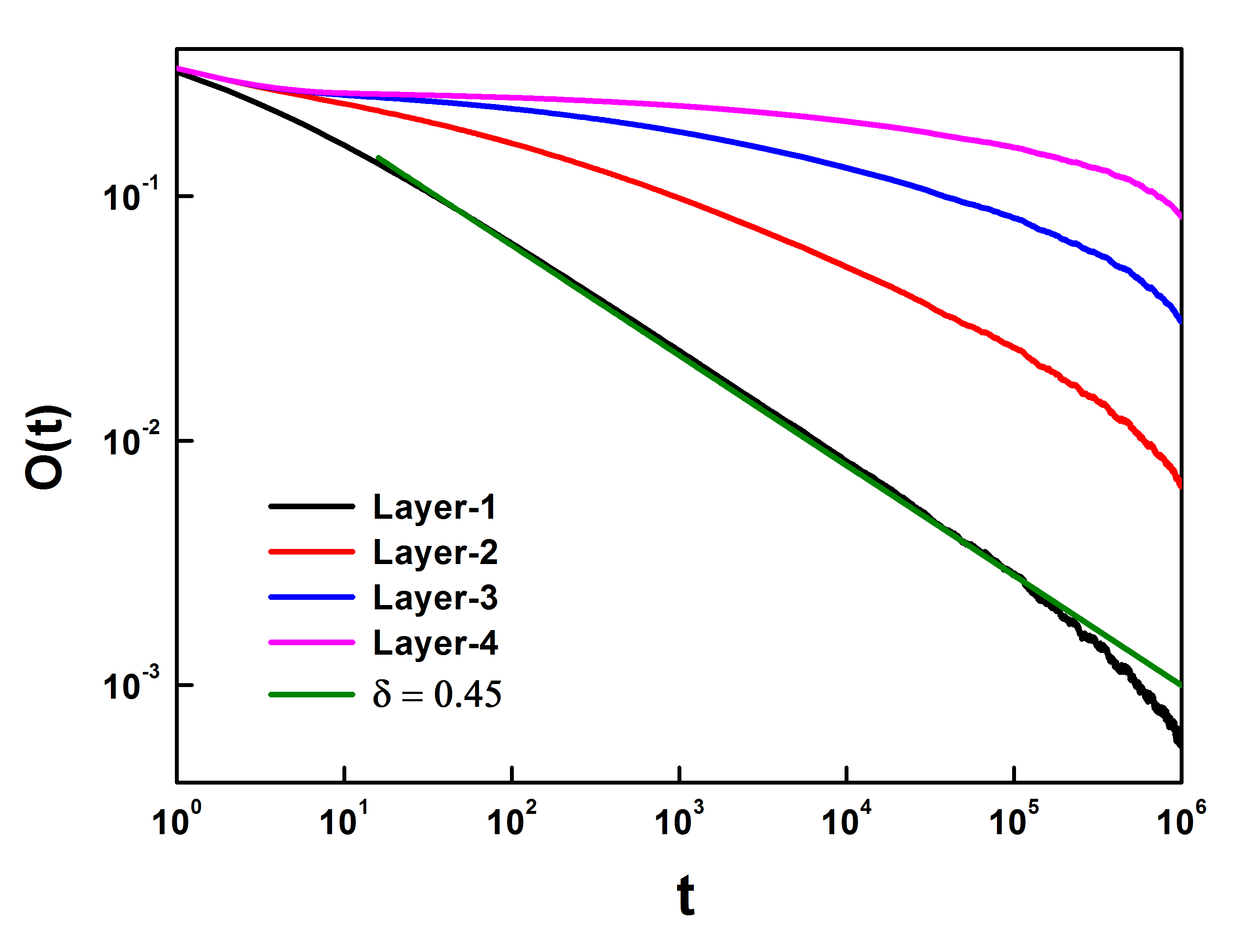
Figure 8: We plot $O_{j}(t)$ as function of time $t$ for 2-D network (from bottom to top) of size $N=2.5\times 10^{3}$ at $p=P_{c}=0.34457$. The decay exponent for first layer is $\delta=0.45$.

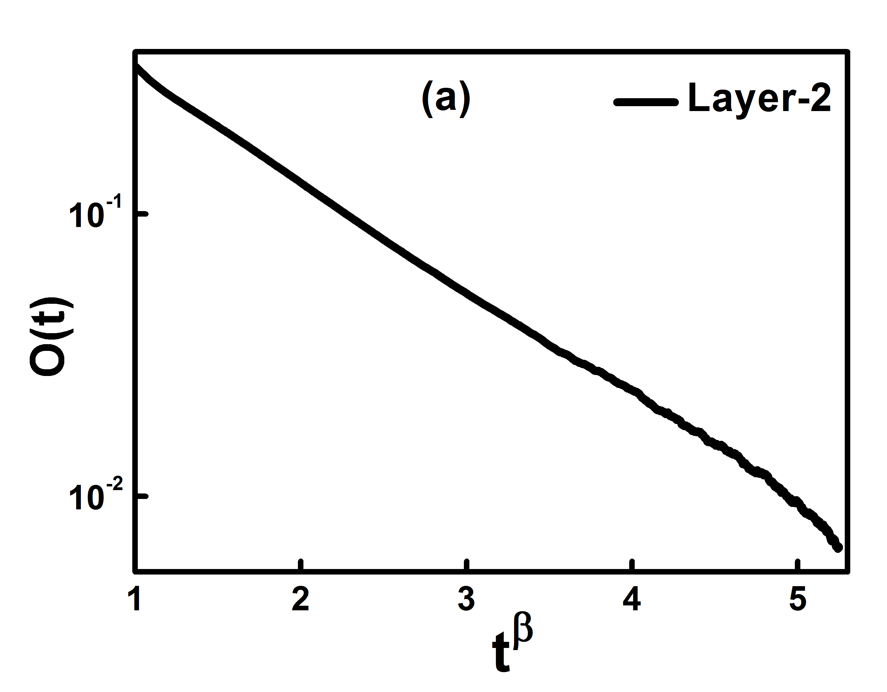
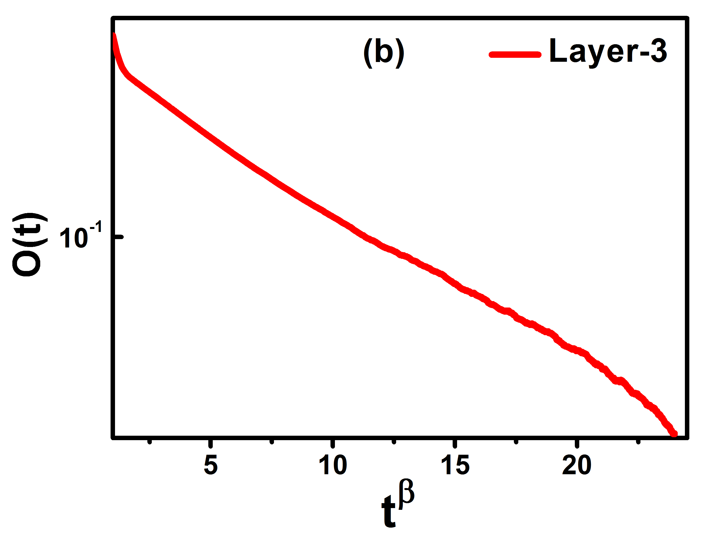
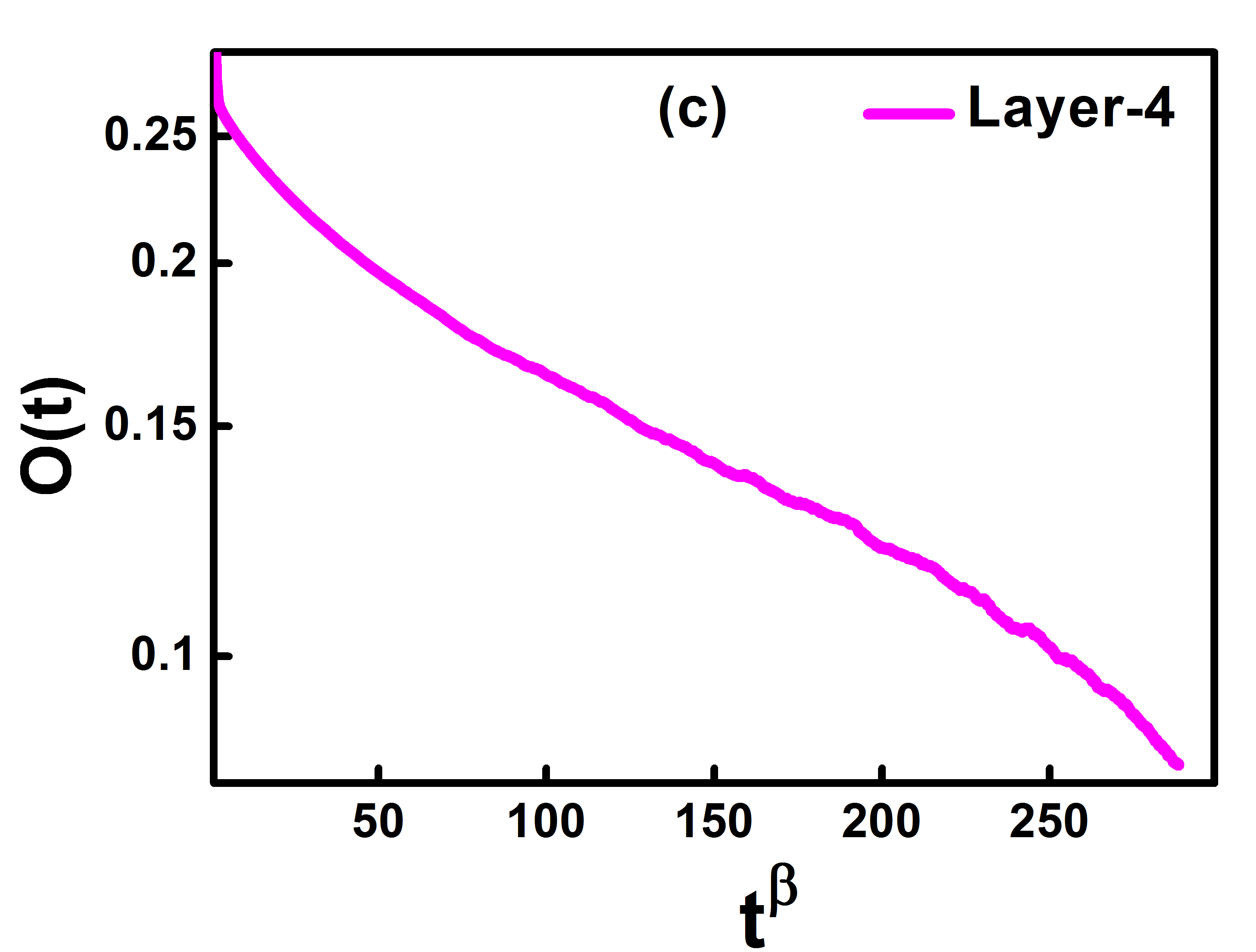
Figure 9: We plot $O_{j}(t)$ vs. $t^{\beta}$ on semi-log scale for $j\neq 1$ at $p=p_{c}$. Data is well fitted by stretched exponential (a) j=2, $\beta=0.12$ (b) j=3, $\beta=0.23$ (c) j=4, $\beta=0.41$

In this paper, we discussed three systems i.e. random system, 1-D, and 2-D system. In these systems, each layer is connected to the layer above it in a unidirectional manner. The top layer has no connection to any other layer. The contact process in this system is defined in the following manner. Any site becomes active with probability $p$ if any of the connected sites is active. The critical point for the top layer is well known and the critical point is expected to be the same for entire network. We compute the fraction of active sites $O_{l}(t)$ in a given layer $l$ as an order parameter.

(a) In a random network, we find that there is a power-law decay of order parameter at each layer for $p=p_{c}$ and the decay exponent is half of the previous layer. Since a well-defined order parameter decay exponent is observed, we compute other exponents such as finite-size scaling and off-critical scaling. We find that the dynamic exponent $z=0.5$ for all layers is not the mean-field exponent. The saturation value of order parameter for various layers scales as $\Delta^{\beta_{l}}$ where $\beta_{l}=\delta_{l}\nu_{\parallel,l}$. Even the value of $\nu_{\parallel,l}\neq 1$ except the first layer which is a departure from mean-field. We propose a system of hierarchy of differential equations that correctly reproduces the behavior at a critical point for all layers, but not the behavior in fluctuating phase.

(b) In 1-D and 2-D networks, the absorbing phase transition in the first layer leads to a power-law decay of order parameter only in the top layer. We find that other layers show a stretched exponential decay. As expected, the power-law decay exponent of the first layer is the same as to DP in 1-D or 2-D lattice. However, the decay is not described by power law for other layers. It is better fitted by the stretched exponential.

ACKNOWLEDGMENTS

PMG thanks DST-SERB (CRG/2020/003993) for financial assistance. MCW thanks the Council of Scientific and Industrial Research (C.S.I.R.), SRF (09/128(0097)/2019-EMR-I).

References

- Nakamura (2003) I. Nakamura, Phys. Rev. E 68, 045104(R) (2003).
- Börner et al. (2007) K. Börner, S. Sanyal, and A. Vespignani, Annu. Rev. Inf. Sci. Technol. 41, 537 (2007).
- Hein et al. (2006) O. Hein, M. Schwind, and W. König, Wirtschaftsinformatik 48, 267 (2006).
- Newman et al. (2011) M. E. Newman, D. Walls, M. Newman, A.-L. Barabási, and D. J. Watts, in The Structure and Dynamics of Networks (Princeton University Press, 2011) pp. 310–320.
- Zhang et al. (2018) H. Zhang, L. Qiu, L. Yi, and Y. Song, in IJCAI, Vol. 18 (2018) pp. 3082–3088.
- Kanawati (2015) R. Kanawati, IEEE Intell. Informatics Bull. 16, 24 (2015).
- Tian et al. (2016) Z. Tian, L. Jia, H. Dong, F. Su, and Z. Zhang, Procedia Eng. 137, 537 (2016).
- Sanz et al. (2014) J. Sanz, C. Y. Xia, S. Meloni, and Y. Moreno, Phys. Rev. X 4, 041005 (2014).
- de Arruda et al. (2017) G. F. de Arruda, E. Cozzo, T. P. Peixoto, F. A. Rodrigues, and Y. Moreno, Phys. Rev. X 7, 011014 (2017).
- Guo et al. (2016) Q. Guo, E. Cozzo, Z. Zheng, and Y. Moreno, Sci. Rep. 6, 1 (2016).
- Gomez et al. (2013) S. Gomez, A. Diaz-Guilera, J. Gomez-Gardenes, C. J. Perez-Vicente, Y. Moreno, and A. Arenas, Phys. Rev. Lett. 110, 028701 (2013).
- Gade and Sinha (2005) P. M. Gade and S. Sinha, Phys. Rev. E 72, 052903 (2005).
- Mahajan et al. (2013) A. V. Mahajan, M. A. Saif, and P. M. Gade, Eur. Phys. J. Spec. Top. 222, 895 (2013).
- Henkel et al. (2008) M. Henkel, H. Hinrichsen, S. Lübeck, and M. Pleimling, Non-equilibrium phase transitions, Vol. 1 (Springer, 2008).
- Edwards (2002) P. M. Edwards, J. Chem. Inf. Comput. Sci. 42, 1270 (2002).
- Ranganathan (2004) A. Ranganathan, Tutoral on L.M. algorithm 11, 101 (2004).