A Semi-Supervised Adaptive Discriminative Discretization Method Improving Discrimination Power of Regularized Naive Bayes

Shihe Wang^a (Shihe.Wang@nottingham.edu.cn), Jianfeng Ren^a (Jianfeng.Ren@nottingham.edu.cn), Ruibin Bai^a (Ruibin.Bai@nottingham.edu.cn)

^a School of Computer Science, University of Nottingham Ningbo China, Ningbo 315100, China

Corresponding Author:
Jianfeng Ren
School of Computer Science, University of Nottingham Ningbo China, Ningbo 315100, China
Email: Jianfeng.Ren@nottingham.edu.cn

Abstract

Recently, many improved naive Bayes methods have been developed with enhanced discrimination capabilities. Among them, regularized naive Bayes (RNB) produces excellent performance by balancing the discrimination power and generalization capability. Data discretization is important in naive Bayes. By grouping similar values into one interval, the data distribution could be better estimated. However, existing methods including RNB often discretize the data into too few intervals, which may result in a significant information loss. To address this problem, we propose a semi-supervised adaptive discriminative discretization framework for naive Bayes, which could better estimate the data distribution by utilizing both labeled data and unlabeled data through pseudo-labeling techniques. The proposed method also significantly reduces the information loss during discretization by utilizing an adaptive discriminative discretization scheme, and hence greatly improves the discrimination power of classifiers. The proposed RNB+, i.e., regularized naive Bayes utilizing the proposed discretization framework, is systematically evaluated on a wide range of machine-learning datasets. It significantly and consistently outperforms state-of-the-art NB classifiers.

1 Introduction

Naive Bayes (NB) has been widely used in many machine-learning tasks because of its simplicity and efficiency [Ren et al., 2022, Kishwar & Zafar, 2023, Gonçales et al., 2022, Lavanya et al., 2021, Zhang et al., 2021, Shaban et al., 2021, Geng et al., 2019, Qorib et al., 2023]. It could well handle different data types such as numerical and categorical ones. Naive Bayes assumes that features are independent conditioned on the classification variable, while such an assumption often does not hold [Wang et al., 2020, Ren et al., 2015a], which may degrade the classification performance. Numerous improved NB classifiers have been developed to alleviate this problem, which can be broadly divided into five categories: structure extension [Wu et al., 2016, Jiang et al., 2016b, Geng et al., 2019], instance selection [Quinlan, 2014, Wang et al., 2015], instance weighting [Jiang et al., 2012, Xu et al., 2019], attribute selection [Zhang et al., 2009, Tang et al., 2016, Jiang et al., 2019a, Chen et al., 2020] and attribute weighting [Zhang et al., 2020, Jiang et al., 2018, Ruan et al., 2020, Zaidi et al., 2013, Jiang et al., 2019b, Yu et al., 2020, Wang et al., 2020].

Among these, attribute weighting NB classifiers comparably perform better [Jiang et al., 2016a, 2018, Ruan et al., 2020, Zaidi et al., 2013, Jiang et al., 2019b, Yu et al., 2020, Wang et al., 2020]. In WANBIA, attributes are weighted differently according to the feature importance using the classification feedback [Zaidi et al., 2013]. In class-specific attribute weighted naive Bayes (CAWNB), different weights are assigned to the attributes of different classes to enhance the discrimination power [Jiang et al., 2019b]. Most recently, regularized naive Bayes has been developed to improve the classification performance by balancing the generalization capability and discrimination power of the classifier automatically through a gradient descent optimization using the classification feedback [Wang et al., 2020]. These methods enhance the discrimination power of NB classifiers by feature weighting, but overlook the issues on data discretization.

The goal of data discretization is to find a set of cut points to optimally discretize numerical attributes, reducing the inconsistency rate while preserving the discriminant information [Sharmin et al., 2019]. However, improving generalization ability by reducing the inconsistency rate and maintaining the discrimination power are two opposite goals. On the one hand, by grouping similar values into one interval, more samples can be used to better estimate the distribution of the interval, leading to better generalization abilities, but at the cost of losing discriminant information. On the other hand, without data discretization, the discriminative ability is retained to the greatest extent, but the generalization ability is poor. A well-designed data discretization method should balance the trade-off between preserving discriminative ability and improving generalization ability.

In literature, many discretizers follow this design principle [Kurgan & Cios, 2004, Fayyad, 1993, Tsai et al., 2008]. In CAIM, a greedy algorithm is utilized to approximately find the global optimum by simultaneously minimizing the number of intervals and maximizing the class-attribute interdependence, but CAIM does not guarantee to find the global optimum [Kurgan & Cios, 2004]. In MDLP, an entropy-based discretization criterion is utilized to select the cut points by maximizing the entropy of the data, which splits the attribute into intervals in a top-down manner [Fayyad, 1993]. To avoid excessive splitting, a stopping criterion is defined. But this stopping criterion often leads to an early stop in the splitting process, very few discretization intervals and hence a significant information loss. Despite all these problems, it is surprising that MDLP is often used in advanced naive Bayes classifiers and yields satisfactory performance [Zaidi et al., 2013, Jiang et al., 2019b, Wang et al., 2020, Zhang et al., 2021].

The aforementioned discretization methods are often known as supervised discretization methods [Kurgan & Cios, 2004, Fayyad, 1993, Tsai et al., 2008], where the class information is utilized to guide the discretization process. In literature, unsupervised methods such as equal-width discretization [Kurgan & Cios, 2004] and equal-frequency discretization [Kurgan & Cios, 2004] are also used, which do not require the class information. The collected data are often unlabeled and labeling data is often expensive because it needs the expert knowledge [Liang et al., 2019]. Hence, there is often a huge amount of unlabeled data, whereas only a small portion is labeled. In this case, a semi-supervised discretization scheme is preferred to utilize both labeled and unlabeled data.

In this paper, we propose a semi-supervised adaptive discriminative discretization (SADD) to address the problem of previous methods, targeting at balancing the discrimination power and generalization ability of NB classifiers. In recent years, semi-supervised methods have been successfully applied in machine learning tasks to improve the generalization ability of models on unseen data and avoid the overfitting problem [Karimi et al., 2022, Hu et al., 2022, Lai et al., 2022a, b, Liang et al., 2019]. In the proposed semi-supervised discretization method, unlabeled data is first assigned a pseudo label by using a simple classification model such as k-Nearest Neighbors (k-NN) classifier [Hu et al., 2022, Liang et al., 2019]. Then, the pseudo-labeled data is integrated with the labeled data to provide more discriminant information for the discretization method. With the help of pseudo-labeled data, the intrinsic data structure could be better discovered in which the discriminative ability and generalization ability of subsequently trained classifiers can be greatly enhanced.

After pseudo-labeling, an adaptive discriminative discretization scheme is proposed in this paper. The proposed semi-supervised framework could better discover the intrinsic data properties, so that the data distribution could be better estimated. Data is often discretized to improve the generalization ability by grouping similar values into one interval, but too few intervals will result in a significant information loss and too few samples in the interval will result in poor generalization performance. The proposed SADD explicitly addresses the problem of early stop in MDLP [Fayyad, 1993] by using an adaptive discriminative discretization scheme, and hence resolves the issue of significant discriminant information loss in MDLP. As a result, each interval has a sufficient number of samples to reliably estimate the likelihood probabilities in naive Bayes so that the naive Bayes can generalize well on unseen data, and a sufficient number of intervals are retained to maintain the discriminant information. In another word, the proposed SADD well balances the discrimination power and generalization ability of the data discretizer.

The proposed SADD is integrated with the recent development of NB classifier, regularized naive Bayes (RNB) [Wang et al., 2020], and the integrated method is named as RNB+. Compared to RNB, the proposed RNB+ well addresses the early stopping problem in data discretization of RNB and preserves the discriminant information of the data, and hence better balances the discrimination power and generalization ability. The proposed methods are evaluated on a wide range of machine-learning datasets for various applications. Experimental results show that the proposed SADD significantly outperforms the widely used discretization methods [Fayyad, 1993, Kurgan & Cios, 2004, Tsai et al., 2008] and the proposed RNB+ significantly outperforms the state-of-the-art NB classifiers [Zaidi et al., 2013, Jiang et al., 2019b, Wang et al., 2020, Zhang et al., 2021].

2 Related Works

We will first review various improvements of naive Bayes classifiers, especially attribute-weighting NB classifiers. Then we will review the advancements in data discretization, especially those applied to NB classifiers.

2.1 Naive Bayes Classifiers

Naive Bayes classifiers have been widely used in many applications [Ren et al., 2022, Kishwar & Zafar, 2023, Gonçales et al., 2022, Lavanya et al., 2021, Zhang et al., 2021, Shaban et al., 2021, Geng et al., 2019, Qorib et al., 2023]. To improve the classification performance, many advanced NB classifiers have been developed, which can be divided into five categories. 1) Structure extension [Wu et al., 2016, Jiang et al., 2016b], by extending the structure of NB to represent the attribute dependencies, in order to alleviate the independence assumption. 2) Instance selection [Quinlan, 2014, Wang et al., 2015], by building a local NB model on a subset of the training instances, to reduce the effect of noisy instances. 3) Instance weighting [Jiang et al., 2012, Xu et al., 2019], which enhances the discrimination power of NB classifiers by assigning a different weight to each instance. 4) Attribute selection [Tang et al., 2016, Jiang et al., 2019a, Chen et al., 2020], to remove the redundant or irrelevant attributes and select the most informative attributes to generate the classification model. 5) Attribute weighting [Jiang et al., 2016a, 2018, Ruan et al., 2020, Zaidi et al., 2013, Jiang et al., 2019b, Yu et al., 2020, Wang et al., 2020], by weighting the attributes differently so that the discriminative attribute has a larger weight and hence the discrimination power is increased.

Among these methods, attribute weighting methods have achieved better performance [Jiang et al., 2016a, 2018, Ruan et al., 2020, Zaidi et al., 2013, Jiang et al., 2019b, Yu et al., 2020, Wang et al., 2020], which can be further divided into filter-based [Lee et al., 2011, Jiang et al., 2016a, 2018, Ruan et al., 2020] and wrapper-based methods [Zaidi et al., 2013, Jiang et al., 2019b, Yu et al., 2020, Wang et al., 2020]. The former determines the attribute weights by measuring the relationship between attributes and class variables in terms of mutual information [Jiang et al., 2018], KL divergence [Lee et al., 2011] or correlation [Jiang et al., 2018]. The latter optimizes the attribute weights iteratively by using the classification feedback, which often achieves better classification performance at a higher computational cost. Zaidi et al. [2013] optimized attribute weights by minimizing the mean squared error between the estimated posterior probabilities and the ones derived from ground-truth labels. Recently, Jiang et al. [2019b] developed a class-specific attribute-weighting NB model, in which different weights are assigned to the attributes of different classes to enhance the discriminative ability [Jiang et al., 2019b]. Very recently, Wang et al. [2020] developed the regularized NB, which optimally balances the discrimination power and generalization ability of the classifier.

2.2 Data Discretization Methods

In naive Bayes classifiers and many other classifiers [Jiang et al., 2016a, 2018, Ruan et al., 2020, Zaidi et al., 2013, Jiang et al., 2019b, Yu et al., 2020, Wang et al., 2020, Zhang et al., 2021], numerical attributes are often discretized to group similar values into one bin, to address the problem that numerical attributes often have lots of noisy samples resulting in poor generalization capabilities. Existing discretization methods can be broadly divided into unsupervised, semi-supervised and supervised methods, depending on whether the class information is used [Ramírez-Gallego et al., 2016]. Unsupervised discretization methods include equal-frequency, equal-width discretization [Kurgan & Cios, 2004], proportional k-interval discretization (PKID) [Yang & Webb, 2001] and fixed frequency discretization (FFD) [Yang & Webb, 2009]. Equal-frequency discretization divides the attribute set into intervals with the same number of instances, while the equal-width discretization divides the attribute set into intervals with the same length [Kurgan & Cios, 2004]. PKID adjusts the number and size of intervals proportional to the number of training instances [Yang & Webb, 2001]. FFD divides the data into intervals with a pre-defined frequency Yang & Webb [2009] Supervised discretization methods include MDLP [Fayyad, 1993], other information-based algorithms [Dougherty et al., 1995, Kurgan & Cios, 2004], and statistical algorithms like ChiMerge [Kerber, 1992], class-attribute interdependence maximization (CAIM) [Kurgan & Cios, 2004] and class-attribute contingency coefficients (CACC) [Tsai et al., 2008]. Semi-supervised discretization methods are comparatively less studied. Bondu et al. [2010] developed a semi-supervised framework based on MODL to exploit a mixture of labeled and unlabeled data. In this paper, we mainly review CAIM [Kurgan & Cios, 2004] and MDLP [Fayyad, 1993] in detail as they follow closely to the design concept of balancing the discrimination power and generalization ability. In CAIM, the boundary point is selected with the maximal interdependence in a top-down manner by using a quanta matrix [Kurgan & Cios, 2004], but the number of generated intervals is too close to the number of classes. To address this problem, Tsai et al. [2008] developed a discretization method based on class-attribute contingency coefficients to prevent the information loss.

Many state-of-the-art NB classifiers such as WANBIA [Zaidi et al., 2013], CAWNB [Jiang et al., 2019b], AIWNB [Zhang et al., 2021] and RNB [Wang et al., 2020] utilize the MDLP criterion [Fayyad, 1993] to discretize numerical attributes in a top-down manner. In MDLP, for each interval, a cut point with the maximum entropy amongst all candidates is selected to split the interval into two, towards the goal of retaining the maximum amount of discriminant information [Fayyad, 1993]. To avoid the poor generalization ability caused by excessive splitting, a stop criterion is designed based on the concept of information encoding in a communication channel [Fayyad, 1993]. MDLP often leads to a good classification performance as it balances the discrimination power and generalization ability. However, as shown later in the next section, the early stopping problem during splitting in MDLP often leads to a huge information loss and hence degrades the performance of subsequent classifiers.

3 Proposed Method

3.1 Problem Analysis of MDLP

Data discretization is crucial to the classification performance. As an entropy-based discretization method with strong theoretical background [Peng et al., 2005, Ren et al., 2014, 2015b, Gao et al., 2018, Sharmin et al., 2019, Flores et al., 2019], MDLP [Fayyad, 1993] has been widely used in many state-of-the-art attribute weighting NB classifiers [Zaidi et al., 2013, Jiang et al., 2019b, Wang et al., 2020, Zhang et al., 2021]. It splits the dynamic range in a top-down manner, i.e., for each attribute, a cut point retaining the maximum amount of discriminant information is selected to divide the current set into two. The discriminant information is measured by the information gain of a cut point $d$ for a given attribute, dividing the current example set $\mathcal{S}$ into two subsets $\mathcal{S}_{1}$ and $\mathcal{S}_{2}$. The information gain $G(\mathcal{S},d)$ is defined as,

$$G(\mathcal{S},d)=E(\mathcal{S})-\frac{|\mathcal{S}_{1}|}{|\mathcal{S}|}E(\mathcal{S}_{1})-\frac{|\mathcal{S}_{2}|}{|\mathcal{S}|}E(\mathcal{S}_{2}),$$ (1)

where $E(\mathcal{S})$ is the class entropy as defined below,

$$E(\mathcal{S})=-\sum_{i=1}^{k}P(C_{i},\mathcal{S})log(P(C_{i},\mathcal{S})).$$ (2)

$P(C_{i},\mathcal{S})$ is the prior probability of class $C_{i}$ in $\mathcal{S}$, and $k$ is the number of classes. The binary split in MDLP is applied recursively if Eqn. (3) holds, and stops otherwise. Intuitively, the stop criterion will prevent excessively splitting the attribute into too many small intervals with too few samples so that the likelihood probabilities can not be reliably estimated.

$$G(\mathcal{S},d)>\theta,$$ (3)

where $\theta$ is the adaptive threshold for discretization,

$$\theta=\frac{log_{2}(N-1)}{N}+\frac{\Delta(\mathcal{S})}{N},$$ (4)

where $N$ is the number of samples in $\mathcal{S}$. $\Delta(\mathcal{S})$ is defined as,

$$\Delta(\mathcal{S})=log_{2}(3^{k}-2)-[kE(\mathcal{S})-k_{1}E(\mathcal{S}_{1})-k_{2}E(\mathcal{S}_{2})],$$ (5)

where $k_{1}$ and $k_{2}$ are the number of classes in $\mathcal{S}_{1}$ and $\mathcal{S}_{2}$, respectively. Empirical study shows that the threshold $\theta$ is often too large compared to the information gain $G(\mathcal{S},d)$ so that the top-down splitting often stops at an early stage. As a result, a huge amount of discriminant information is lost.

To explore the root cause of this early stop, we take a close examination of the adaptive threshold $\theta$ defined in Eqn. (4). Empirical study shows that the first term $\frac{log_{2}(N-1)}{N}$ dominates the adaptive threshold $\theta$, while the second term $\frac{\Delta(\mathcal{S})}{N}$ is a relatively small positive value. We further analyze $\frac{log_{2}(N-1)}{N}$ by plotting it against $N$ as shown in Fig. 2.

Apparently when $N$ is large, $\frac{log_{2}(N-1)}{N}$ is relatively small and the data could be easily split into intervals in a top-down manner. As the split continues, the number of samples $N$ in the interval becomes smaller, leading to a large $\frac{log_{2}(N-1)}{N}$, and hence it is more difficult to split. This decision criterion follows the design principle of balancing the discriminative ability and generalization ability, and works well when $N$ is large. However, for small $N$, $\frac{log_{2}(N-1)}{N}$ is relatively large and hence many attributes with a small number of samples may not split at all at the very beginning. In this case, the attribute is discretized into one bin only, and the discriminant information residing in the attribute is totally lost.

3.2 Overview of Proposed SADD Framework for Regularized Naive Bayes

As shown in the previous subsection, the early stopping problem in MDLP may result in a significant loss of discriminant information during discretization. In a broader sense, data discretization helps to improve the generalization ability of naive Bayes classifiers by grouping similar values into one bin, whereas excessive grouping (such as an early stop in MDLP) will result in a significant information loss. It is hence crucial for a data discretizer to balance the generalization ability and discrimination power. Furthermore, supervised discretization methods such as MDLP [Fayyad, 1993] and CAIM [Kurgan & Cios, 2004] are not capable of handling unlabeled data without any adaptation, and hence the information residing in unlabeled data can’t be fully exploited by those supervised discretization methods. Thus, a semi-supervised discretization method exploiting both labeled and unlabeled data is needed.

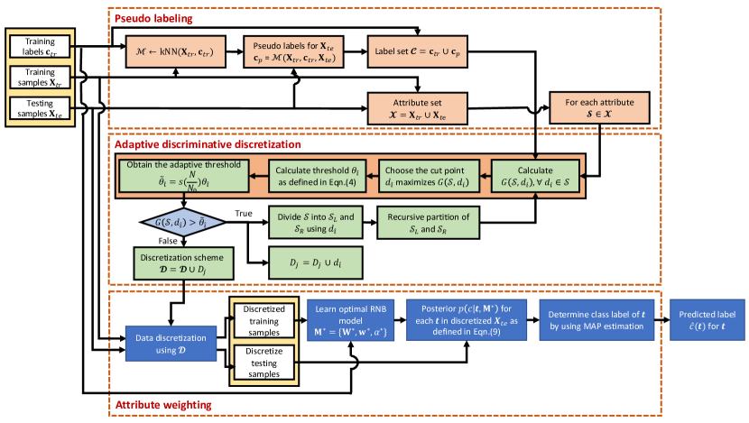
Figure 1: The proposed SADD for regularized naive Bayes. Firstly, the pseudo labels for unlabeled testing samples are generated by using k-NN. Then, both training data and testing data are used to derive the discretization scheme balancing the generalization capability and discrimination power. The derived SADD scheme is then applied to transform the numerical attributes into discrete ones, improving the generalization ability while attaining the discrimination power of the classifier. Finally, the regularized naive Bayes is integrated with the proposed SADD to derive the optimal attribute weights and determine the class labels by using MAP estimation.

To address these problems, we propose a Semi-supervised Adaptive Discriminative Discretization (SADD) method for regularized naive Bayes (The integrated method is also known as RNB+), as shown in Fig. 1. 1) First of all, a semi-supervised technique is designed to generate the pseudo labels for the unlabeled data, so that the intrinsic data properties in both labeled and unlabeled data could be exploited to better estimate the data statistics. In this paper, the k-NN classifier is applied to generate the pseudo labels. 2) Secondly, an adaptive discriminative discretization scheme is designed to discretize the attribute set, where a new adaptive thresholding strategy is designed to balance the number of intervals required to retain the sufficient discrimination power and the number of samples in an interval to retain the sufficient generalization ability. 3) We consider the trade-off between the generalization ability and discrimination power not only in data discretization, but also in classifier design such as feature weighting. Following this design principle, the proposed SADD is integrated with regularized naive Bayes, in which the attributes are weighted automatically balancing the discrimination power and generalization ability of the classifier.

3.3 Proposed Semi-supervised Adaptive Discriminative Discretization

3.3.1 Pseudo-labeling

Semi-supervised techniques have proven to be a powerful paradigm for utilizing unlabeled data to improve the generalization ability of learning models relying solely on labeled data [Karimi et al., 2022, Hu et al., 2022, Lai et al., 2022a, b]. Among various semi-supervised methods, pseudo-labeling techniques are effective to tackle the problem, which can be easily integrated with traditional supervised classification algorithms [Liang et al., 2019]. More specifically, let $\bm{X}_{l}$ be the labeled data with class variables $\bm{c}_{l}$ and $\bm{X}_{u}$ be the unlabeled data, the pseudo labels $\bm{c}_{p}$ for $\bm{X}_{u}$ can be derived by,

$$\bm{c}_{p}=\mathcal{M}(\bm{X}_{l},\bm{c}_{l},\bm{X}_{u}),$$ (6)

where $\mathcal{M}$ represents a pseudo-labeling algorithm. There are two main approaches to generate the pseudo labels: single-classifier and multi-classifier methods. In a single-classifier model, the pseudo label for each unlabeled instance is derived by using only one classification model. In contrast, multi-classifier model utilizes the majority voting rule to decide the pseudo label by using several classifiers. To keep the simplicity and effectiveness of the proposed framework, the k-nearest neighbors (k-NN) classifier is applied to generate the pseudo labels for unlabeled data. Then, the pseudo-labeled data and labeled data are combined to better discover the intrinsic data properties and better estimate the data statistics.

3.3.2 Adaptive Discriminative Discretization

To address the early stopping problem in previous discretization methods [Fayyad, 1993], we propose an adaptive discriminative discretization. More specifically, we aim to lower the adaptive threshold used in Eqn. (3), especially for small datasets with relatively small $N$, in order to prevent the early stop and the significant loss of discriminant information during discretization. On the other hand, the new threshold $\tilde{\theta}$ can not be too small. If $\tilde{\theta}$ is approaching zero, each distinct value will become a separate interval, which results in no information loss, but may lead to a poor estimation of data distribution due to insufficient samples in each small interval. Bearing all these in mind, we propose the new threshold $\tilde{\theta}$ as defined below:

$$\tilde{\theta}=s\left(\frac{N}{N_{0}}\right)\theta,$$ (7)

where $s(x)=1/(1+e^{-x})$ is the sigmoid function and $N_{0}$ is a constant. As $\frac{N}{N_{0}}$ is non-negative, it is easy to show that $s(\frac{N}{N_{0}})\in(0.5,1)$. $N_{0}$ is used to judge whether there are sufficient samples in the interval. If $N\gg N_{0}$, i.e., there are sufficient samples, $s(\frac{N}{N_{0}})\approx 1$. In this case, although $s(\frac{N}{N_{0}})$ is relatively large, $\theta$ is relatively small, and $\tilde{\theta}$ is small enough so that the top-down split could continue, and the resulting intervals will have sufficient samples to reliably estimate the likelihood probabilities. If $N\approx N_{0}$, $s(\frac{N}{N_{0}})\approx 0.73$, i.e., a significantly lower threshold $\tilde{\theta}$ will be used in the top-down discretization compared to the threshold $\theta$ defined in Eqn. (4). Consequently, it will encourage further splitting of the interval and hence retain more discriminant information. To prevent excessive splitting, the proposed method has a safeguard mechanism. More specifically, when $N\ll N_{0}$, $s(\frac{N}{N_{0}})\approx 0.5$, i.e., the maximum reduction of the threshold $\tilde{\theta}$ from $\theta$ is 50%.

Figure 2: Plot of $\frac{log_{2}(N-1)}{N}$ and its adaptive version $s(\frac{N}{N_{0}})\frac{log_{2}(N-1)}{N}$ with different values of $N_{0}$. When $N$ is small, the new adaptive threshold is about half of $\frac{log_{2}(N-1)}{N}$, which prevents a possible early stop in the top-down split.

To further illustrate the effect of the adaptive threshold in the proposed method, we plot the value of the adaptive version of $\frac{log_{2}(N-1)}{N}$ after multiplying it with $s(\frac{N}{N_{0}})$ for different $N_{0}$, as shown in Fig. 2. With the small number of samples in an interval, the threshold is greatly decreased from about 0.4 to 0.2 to encourage further splitting, especially for small datasets. When $N$ is large, the new adaptive threshold is smaller than the original one, but very close to it, to encourage the split. In addition, the proposed method is insensitive to the choice of $N_{0}$. As shown in Fig. 2, the new thresholds for $N_{0}=100$ and $N_{0}=2000$ are quite close when $N$ is small. For large $N$, the difference does not matter so much as the set will be split into smaller ones anyway. In summary, the proposed SADD could effectively prevent the early stop during data discretization, as well as the excessive split. The proposed SADD algorithm is summarized in Algorithm 1.

Algorithm 1 The proposed SADD algorithm

1:Training data $\bm{X}_{l}$ with class $\bm{c}_{l}$ and testing data $\bm{X}_{u}$

2:Discretization scheme $\bm{\mathcal{D}}\leftarrow\{\mathcal{D}_{1},\mathcal{D}_{2},...,\mathcal{D}_{m}\}$ for $m$-dimensional features

3:$\bm{c}_{p}\leftarrow\mathcal{M}(\bm{X}_{l},\bm{c}_{l},\bm{X}_{u})$ $\triangleright$ Derive pseudo labels using Eqn. (6)

4:$\bm{\mathcal{X}}\leftarrow\bm{X}_{l}\cup\bm{X}_{u}$ $\triangleright$ $\bm{\mathcal{X}}$ is the set of samples

5:$\bm{\mathcal{C}}\leftarrow\bm{c}_{l}\cup\bm{c}_{p}$ $\triangleright$ $\bm{\mathcal{C}}$ is the set of labels

6:$\bm{\mathcal{D}}\leftarrow\emptyset$ $\triangleright$ Initialize $\bm{\mathcal{D}}$ as an empty set

7:for each $\mathcal{X}_{j}\in\bm{\mathcal{X}}$ do

8:    $\mathcal{D}_{j}\leftarrow\emptyset$ $\triangleright$ $\mathcal{D}_{j}$ is the discretization scheme for $\mathcal{X}_{j}$

9:    $\mathcal{S}\leftarrow\mathcal{X}_{j}$ $\triangleright$ $\mathcal{S}$ is the set of samples to be discretized

10:    procedure Partition($\mathcal{S},\bm{\mathcal{C}}$) $\triangleright$ Procedure to partition $\mathcal{S}$ using $\bm{\mathcal{C}}$

11:        if $|\mathcal{S}|$ ==1 then $\triangleright$ If there is only one sample in $\mathcal{S}$, return

12:           return

13:        end if

14:        Calculate $G(\mathcal{S},d_{i}),\forall d_{i}\in\mathcal{S}$, as defined in Eqn. (1).

15:        Choose the cut point $d_{\hat{i}}$, $\hat{i}=\mathop{\arg\max}_{i}{G(\mathcal{S},d_{i})},\forall d_{i}\in\mathcal{S}$.

16:        Calculate the threshold $\theta_{\hat{i}}$ using Eqn. (4) for the cut point $d_{\hat{i}}$.

17:        Calculate the new adaptive threshold $\tilde{\theta}_{\hat{i}}=s\left(\frac{N}{N_{0}}\right)\theta_{\hat{i}}$.

18:        if $G(\mathcal{S},d_{\hat{i}})>\tilde{\theta}_{\hat{i}}$ then $\triangleright$ The SADD stop criterion

19:           $\mathcal{D}_{j}\leftarrow\mathcal{D}_{j}\cup d_{\hat{i}}$ $\triangleright$ Insert $d_{\hat{i}}$ into discretization scheme $\mathcal{D}_{j}$

20:           $\mathcal{S}_{L}\leftarrow\mathcal{S}<d_{\hat{i}}$ $\triangleright$ Divide $\mathcal{S}$ into the set smaller than $d_{\hat{i}}$

21:           $\mathcal{S}_{R}\leftarrow\mathcal{S}\geq d_{\hat{i}}$ $\triangleright$ Divide $\mathcal{S}$ into the set not smaller than $d_{\hat{i}}$

22:           Partition($\mathcal{S}_{L},\bm{\mathcal{C}}$) $\triangleright$ Recursively partition $\mathcal{S}_{L}$ using $\bm{\mathcal{C}}$

23:           Partition($\mathcal{S}_{R},\bm{\mathcal{C}}$) $\triangleright$ Recursively partition $\mathcal{S}_{R}$ using $\bm{\mathcal{C}}$

24:        end if

25:    end procedure

26:    $\bm{\mathcal{D}}\leftarrow\bm{\mathcal{D}}\cup\mathcal{D}_{j}$ $\triangleright$ Add the discretization scheme $\mathcal{D}_{j}$ into $\bm{\mathcal{D}}$

27:end for

28:return $\bm{\mathcal{D}}$

In the first step of Algorithm 1, pseudo labeling, a k-NN classification model $\mathcal{M}$ is generated by using the labeled training data and used to derive the pseudo labels $\bm{c}_{p}$ for unlabeled testing data using Eqn. (6). Then, the attribute set $\bm{\mathcal{X}}$ and label set $\bm{\mathcal{C}}$ are derived by combining the labeled training data with pseudo-labeled testing data. Then the attributes $\mathcal{X}_{j}\in\bm{\mathcal{X}}$ are discretized one at a time. The procedure PARTITION is used to find the optimal cut point $d_{\hat{i}}$ to divide the current sample set $\mathcal{S}$ into two sets $\mathcal{S}_{L}$ and $\mathcal{S}_{R}$, where $\hat{i}=\mathop{\arg\max}_{i}{G(\mathcal{S},d_{i})},\forall d_{i}\in\mathcal{S}$ and $G(\mathcal{S},d_{i})$ is the information gain defined in Eqn. (1). Then, the PARTITION procedure is recursively applied on $\mathcal{S}_{L}$ and $\mathcal{S}_{R}$ to find the optimal cut point to further discretize the attribute. The recursive partition continues as long as the following condition holds:

$$G(\mathcal{S},d_{\hat{i}})>\tilde{\theta}_{\hat{i}},$$ (8)

where $\tilde{\theta}_{\hat{i}}=s\left(\frac{N}{N_{0}}\right)\theta_{\hat{i}}$ is the newly defined adaptive threshold, $\theta_{\hat{i}}$ is the threshold defined in Eqn. (4) for the cut point $d_{\hat{i}}$ and $s(\cdot)$ is the sigmoid function. The discretization scheme $\mathcal{D}_{j}$ for attribute $\mathcal{X}_{j}$ is updated as,

$$\mathcal{D}_{j}\leftarrow\mathcal{D}_{j}\cup d_{\hat{i}}.$$ (9)

For each attribute, the proposed SADD utilizes a greedy hierarchical splitting algorithm to generate a tree-like discretization scheme, as summarized in Algo. 1. It can be shown that the time complexity is $O(n\log{n})$ for each attribute, where $n$ is the number of samples. The total time complexity for $m$ attributes is hence $O(mn\log{n})$.

3.4 Discussion and Analysis

Table 1: The comparisons of the number of intervals (Num.) and the mutual information (MI), after data discretization by the proposed SADD and MDLP [Fayyad, 1993] on all numerical attributes of the “Vowel” dataset.

	Proposed SADD		MDLP
	MI	Num.	MI	Num.
$A_{1}$	1.0921	18	0.9596	8
$A_{2}$	1.2180	19	1.0875	9
$A_{3}$	0.2998	8	0.1198	3
$A_{4}$	0.4488	7	0.3545	4
$A_{5}$	0.5909	14	0.4104	4
$A_{6}$	0.4347	11	0.2759	4
$A_{7}$	0.3287	7	0.2146	3
$A_{8}$	0.2447	7	0.1685	3
$A_{9}$	0.3009	7	0.1796	3
$A_{10}$	0.0527	2	0	1
AVG	0.5011	10	0.3770	4.2

As discussed early, the proposed SADD could effectively prevent the information loss of MDLP. To further analyze this, a case study is presented in Table 1, which shows the number of intervals (Num.) and the mutual information (MI) on the “Vowel” dataset after discretization by MDLP [Fayyad, 1993] and the proposed SADD, respectively. The dataset contains 10 numerical attributes and 11 classes. Most numerical attributes are discretized into 3-4 intervals by MDLP, which can not effectively differentiate 11 classes. After applying the proposed SADD, more intervals could be obtained and hence less discriminant information is lost, as shown in Table 1. The proposed SADD can effectively prevent information loss and generate a discretization scheme with a better trade-off between the number of intervals and the number of samples in the intervals. On the one hand, more intervals will retain more discriminant information, but lead to a poor generalization ability as there are too few samples in an interval to reliably estimate the data distribution. On the other hand, too few intervals may result in a huge discriminant information loss, as shown in the early stopping case of MDLP.

3.5 Proposed RNB+

MDLP has been widely used in many state-of-the-art naive Bayes classifiers, e.g., AIWNB [Zhang et al., 2021], WANBIA [Zaidi et al., 2013], CAWNB [Jiang et al., 2019b] and RNB [Wang et al., 2020]. As shown previously, MDLP may result in a huge information loss and hence the SADD is proposed to address this problem. In this section, we describe how to integrate the proposed SADD with RNB to boost the classification performance of NB classifiers. The integrated method is named as RNB+. We first discretize the data using the proposed SADD so that the data distribution could be better estimated, and then use RNB as the classifier.

We have shown that the proposed SADD could well balance the generalization ability and discrimination power during data discretization. Now we show how the proposed RNB+ achieves a better trade-off during attribute weighting. To alleviate the conditional independence assumption of NB classifiers, attribute weighting techniques have been widely used in NB classifiers and achieved remarkable performance [Zaidi et al., 2013, Jiang et al., 2019b, Wang et al., 2020, Zhang et al., 2021]. In WANBIA, the same weight is assigned to the attributes in different classes [Zaidi et al., 2013], while in CAWNB, a class-specific weight is assigned to each attribute to capture more data characteristics [Jiang et al., 2019b]. But the model complexity increases with more attribute weights, and CAWNB hence may overfit to the data, especially for small datasets. To alleviate this problem, regularized naive Bayes has been recently developed, which regularizes CAWNB by adding a simpler model, i.e., WANBIA, to penalize the model complexity [Wang et al., 2020].

More specifically, in RNB, the target is to find the optimal model parameters $\bm{M}$ =$\{\bm{W},\bm{w},\alpha\}$ to minimize the difference between the posterior derived from the ground-truth label and the estimated posterior for a given instance $\bm{x}$,

$$P(c|\bm{x},\bm{M})=\alpha P_{D}(c|\bm{x},\bm{W})+(1-\alpha)P_{I}(c|\bm{x},\bm{w}),$$ (10)

where $P_{D}(c|\bm{x},\bm{W})$ is the posterior where attributes are weighted on a class-specific basis and $\bm{W}$ is the weight matrix. $P_{I}(c|\bm{x},\bm{w})$ is the posterior where attributes are weighted the same for all classes and $\bm{w}$ is the weight vector. $P_{D}(c|\bm{x},\bm{W})$ is a more complex model that could provide more discrimination power, whereas $P_{I}(c|\bm{x},\bm{w})$ is a simpler model that can provide better generalization ability. In RNB, the optimal model parameters $\bm{M^{*}}$ are derived through a gradient-descent algorithm, and the discrimination power and generalization ability are automatically balanced by optimizing $\alpha$ [Wang et al., 2020]. Finally, the predicted label for each test instance $\bm{t}$ is obtained by using the MAP estimation as follows:

$$\hat{c}(\bm{t})=\mathop{\arg\max}_{c\in C}P(c|\bm{t},\bm{M}^{*}),$$ (11)

where $C$ is the set of labels for all classes.

The categorical attributes and numerical attributes are often mixed and NB classifiers can generate a probabilistic model on both data types. However, the numerical attributes often have a large number of distinct values so that the likelihood probability estimated from the frequency of instances with a particular value $x_{i}$ in the $j$-th attribute given the class $c$, $P(A_{j}=x_{i}|c)$, can be extremely small. The estimation of $P(A_{j}=x_{i}|c)$ may not be reliable due to very few training instances. To address this problem, discretization methods have been developed by grouping similar values into one interval and then sufficient training instances can be used to reliably estimate the likelihood probability. However, many discretization methods, e.g., MDLP [Fayyad, 1993] in the state-of-the-art NB classifiers [Zaidi et al., 2013, Jiang et al., 2019b, Zhang et al., 2021, Wang et al., 2020], can’t generate a proper discretization scheme and may lead to the huge information loss. Thus, RNB+ is proposed to alleviate this problem and retain the discriminative ability from discretization perspective. As shown later in the experiments, the proposed RNB+ significantly outperforms the state-of-the-art NB classifiers such as RNB [Wang et al., 2020], WANBIA [Zaidi et al., 2013], CAWNB [Jiang et al., 2019b] and AIWNB [Zhang et al., 2021].

4 Experimental Results

4.1 Experimental Settings

The experiments are divided into two parts under NB classification framework [Webb, 2003]. The proposed SADD is firstly compared with other discretization methods including four supervised discretization, MDLP [Fayyad, 1993], CAIM [Kurgan & Cios, 2004], CACC [Tsai et al., 2008] and ChiMerge [Kurgan & Cios, 2004], and four unsupervised discretization, Equal-Frequency [Kurgan & Cios, 2004], Equal-Width [Kurgan & Cios, 2004] PKID [Yang & Webb, 2001] and FFD [Yang & Webb, 2009]. Then, the proposed RNB+ is compared with RNB [Wang et al., 2020], WANBIA [Zaidi et al., 2013], CAWNB [Jiang et al., 2019b] and AIWNB [Zhang et al., 2021], which are four recent attribute-weighting NB classifiers. All the competitors are summarized in Table 2. The experimental results of PKID [Yang & Webb, 2001] and FFD [Yang & Webb, 2009] are obtained by using the popular data mining tool, KEEL [Alcalá-Fdez et al., 2009]. The other competitors are implemented by using MATLAB. In the proposed SADD, k-NN classifier with Euclidean distance is used in pseudo-labeling, where the optimal $k$ is tuned by using the validation set. Specifically, one out of nine folds of the training data is randomly selected as the validation set. The optimal $k$ is derived by using a grid search that produces the highest classification accuracy on the validation set.

Table 2: Description of competitors: six popular discretization methods and four state-of-the-art NB classifiers.

Discretization methods
MDLP	Supervised entropy-based top-down discretization
CAIM	Supervised statistical top-down discretization
CACC	Supervised statistical top-down discretization
ChiMerge	Supervised statistical bottom-up discretization
Equal-W	Unsupervised top-down discretization
Equal-F	Unsupervised top-down discretization
PKID	Unsupervised top-down discretization
FFD	Unsupervised top-down discretization
Naive Bayes methods
WANBIA	Wrapper-based class-independent attribute weighting
CAWNB	Wrapper-based class-specific attribute weighting
AIWNB	Filter-based attribute and instance weighting
RNB	Wrapper-based regularized attribute weighting

The comparison experiments are conducted on a set of machine-learning datasets in various domains such as healthcare, biology, disease diagnosis and business. All the datasets are extracted from the UCI machine learning repository . Among them, 12 datasets were used in CACC [Tsai et al., 2008] and the rest of them are selected to enrich the comparison experiments. The number of instances is distributed between 150 and 21048 and the number of attributes is between 4 and 520. The numerical attributes and categorical attributes are mixed in the datasets. Some datasets have missing values, which are replaced by the mean of corresponding numerical attributes or mode of categorical attributes. These 31 benchmark datasets provide a comprehensive evaluation of the proposed SADD and RNB+. The datasets are summarized in Table 3.

Table 3: Most of the datasets are collected from real-world problems in various domains. The number of instances is distributed between 150 and 19020, which provides a comprehensive evaluation on different sizes of datasets. The number of attributes and classes on these datasets are significantly different. Some datasets contain missing values which present real-world difficulties when collecting the data. For the entry $u(v)$ in “Attribute”, $u$ denotes the total number of attributes and $v$ denotes the number of categorical attributes.

Dataset	Instance	Attribute	Class	Missing values
Iris	150	4	3	N
Parkinson	195	23	2	N
Seeds	210	7	3	N
Glass	214	10	6	N
Heart	270	13(7)	2	N
Ecoli	336	8	8	N
Bupa	345	6	2	N
Ionophere	351	34(2)	2	N
Movement	360	90	15	N
ILPD	583	10	2	N
Breast	699	9	2	Y
Pima	768	8	2	N
Vowel	990	13	11	N
Biodegradation	1055	41	2	N
Mice Protein	1080	82	8	Y
Yeast	1484	10	8	N
Mfeat-fac	2000	216	10	N
Cardio	2126	23	10	N
Madelon	2600	500	2	N
Spambase	4601	57	2	N
Wave	5000	40	3	N
Wall-Following	5456	24	4	Y
Page-Block	5473	10	5	N
Opdigit	5620	64	10	N
Satellite	6435	36	6	N
Wine	6497	11	7	N
Musk	6598	166	2	N
Anuran	7195	22	4	N
Pendigit	10992	16	10	N
Magic	19020	10	2	N
IndoorLoc	21048	520	3	N

4.2 Comparisons to State-of-the-art Discretization Methods

The proposed SADD is compared with MDLP [Fayyad, 1993], CAIM [Kurgan & Cios, 2004], CACC [Tsai et al., 2008], ChiMerge [Kerber, 1992], Equal-W [Kurgan & Cios, 2004], Equal-F [Kurgan & Cios, 2004], PKID [Yang & Webb, 2001] and FFD [Yang & Webb, 2009] based on the NB classifier [Webb, 2003]. Table 4 summarizes the comparisons to these discretization methods. The classification accuracy of each algorithm on each dataset is derived via stratified 10-fold cross-validation, following the same evaluation protocol used in [Jiang et al., 2019b, Zaidi et al., 2013, Zhang et al., 2021, Wang et al., 2020]. The symbol $\bullet$ in Table 4 indicates that the proposed method significantly outperforms its competitors with a one-tailed t-test at the significance level of $p=0.05$. The average classification accuracies of all algorithms over all the datasets are summarized at the bottom, which can provide a straightforward comparison of different methods. The hyper-parameter $N_{0}$ in the proposed SADD is set to 2000 empirically.

Table 4: Comparisons between the proposed SADD and other discretization methods such as MDLP [Fayyad, 1993], CAIM [Kurgan & Cios, 2004], CACC [Tsai et al., 2008], ChiMerge [Kerber, 1992], Equal-W (EW) [Kurgan & Cios, 2004], Equal-F (EF) [Kurgan & Cios, 2004], PKID [Yang & Webb, 2001] and FFD [Yang & Webb, 2009] based on the NB classifier [Webb, 2003]. The proposed SADD achieves an average performance gain of 3.11% compared with MDLP, and the performance gain is 2.80% on average compared with previously best performed method, CAIM.

Dataset	SADD	MDLP	CAIM	CACC	ChiMerge	EW	EF	PKID	FFD
Iris	96.00±4.42	92.67±6.29	94.00±5.54	93.33±6.67	78.67±9.80	94.67±6.53	92.67±8.14	91.33±9.45	93.33±6.67
Parkinson	84.02±5.65	79.46±4.69	81.44±7.29	82.46±6.79	81.02±9.18	79.94±6.41	80.35±7.25	77.26±9.90	77.26±7.84
Seeds	90.95±6.19	87.14±4.29	86.67±5.13	87.62±5.30	80.95±4.26	91.43±5.13	88.57±5.71	90.00±8.64	87.62±8.83
Glass	74.29±4.82	72.03±8.65	72.92±9.36	65.25±11.14	66.40±10.08	60.75±7.68	68.24±9.01	65.35±8.78	65.71±10.17
Heart	83.70±8.64	83.70±8.64	83.33±8.16	80.74±6.58	83.70±9.40	84.44±7.73	82.96±8.31	82.96±4.74	83.70±3.78
Ecoli	86.62±4.38	83.10±4.22	81.46±5.58	82.47±5.97	83.38±6.43	85.10±4.26	84.28±5.64	81.58±7.04	82.45±3.05
Bupa	65.76±10.42	53.27±9.52	65.24±6.98	63.24±6.30	64.03±8.58	62.61±8.22	58.55±7.53	61.73±7.41	62.87±8.43
Ionophere	90.62±5.19	89.52±5.12	88.64±4.11	88.92±4.40	75.83±6.21	90.32±4.41	89.77±5.47	89.16±6.11	89.17±5.09
Movement	77.77±6.72	62.10±7.37	71.97±7.94	71.14±7.41	71.41±6.83	70.32±7.17	72.18±6.59	64.87±8.37	67.37±10.45
ILPD	67.05±4.18	64.82±4.45	65.51±4.28	66.03±4.19	65.00±2.68	67.75±2.18	67.40±4.27	67.56±4.89	68.09±2.91
Breast	97.42±1.41	97.14±1.43	97.28±1.50	97.28±1.50	95.85±2.67	97.42±1.55	97.42±1.67	97.43±1.90	97.43±1.90
Pima	76.82±4.34	73.69±4.70	74.21±5.80	74.21±3.92	72.26±5.17	77.21±2.80	74.61±3.61	74.82±4.37	75.35±4.80
Vowel	75.76±4.93	59.09±4.45	64.34±5.27	60.71±6.69	61.11±3.23	67.58±4.87	64.24±5.15	89.63±1.37	60.00±6.69
Biodegradation	81.89±2.80	80.85±2.76	81.70±2.48	81.70±2.75	78.67±4.12	80.19±2.08	81.04±3.19	80.38±3.22	80.00±3.10
Mice Protein	98.06±0.77	93.98±2.60	93.34±2.63	91.67±2.60	92.40±3.55	94.63±2.56	93.05±2.61	93.14±2.05	93.79±2.34
Yeast	59.79±3.89	57.15±3.56	57.49±3.54	56.01±2.88	58.23±4.60	58.64±4.80	55.68±4.93	54.31±2.71	53.57±2.81
Mfeat-fac	94.80±1.95	93.15±2.15	93.70±2.02	93.70±2.23	93.15±2.08	93.3±2.35	92.70±2.50	92.15±2.08	82.79±2.42
Cardio	81.19±1.41	79.68±1.66	80.34±1.78	79.35±1.38	78.12±1.83	79.25±1.61	77.80±2.10	80.15±1.76	81.28±2.76
Madelon	64.65±3.79	61.92±3.34	58.69±2.85	50.00±0.00	58.96±3.98	50.00±0.00	50.00±0.00	55.35±2.47	52.92±3.62
Spambase	90.18±1.72	89.63±1.45	89.85±1.53	90.00±1.63	89.42±1.01	85.53±1.97	89.87±1.41	95.60±0.85	89.33±1.39
Wave	80.70±1.00	80.18±1.00	80.60±1.30	80.32 ± 1.28	78.80±1.04	80.16±0.83	80.24±0.86	79.10±1.60	78.60±1.18
Wall-Following	90.96±0.96	89.24±1.29	88.11±1.06	87.81±1.11	71.15±1.60	80.96±1.41	84.26±1.33	60.91±3.62	86.33±1.42
Page-Block	93.93±1.41	93.62±1.62	93.17±1.25	93.79±1.22	91.25±1.18	92.54±0.80	88.86±1.57	91.78±1.07	92.98±0.81
Opdigit	92.65±0.51	92.38±0.40	92.22±0.64	92.31±0.82	91.76±0.95	92.46±0.74	91.80±0.93	92.19±1.16	92.15±1.15
Satellite	82.45±1.46	82.14±1.40	82.02±1.43	82.08±1.40	79.52±1.55	81.18±1.16	81.15±1.31	82.10±1.43	82.14±1.49
Wine	50.42±1.00	49.19±1.42	49.92±0.86	50.99±1.62	48.47±1.49	49.42±1.46	47.87±1.07	51.82±1.43	53.21±1.78
Musk	92.98±0.79	91.76±0.93	85.50±1.54	89.83±0.75	81.60±2.05	84.18±1.85	83.62±1.54	91.13±0.78	61.68±1.61
Anuran	90.62±1.09	89.92±1.24	89.42±1.29	89.26±1.41	81.86±1.38	89.33±1.30	89.01±1.00	89.41±1.25	88.27±1.57
Pendigit	88.43±0.61	88.10±0.84	87.92±0.72	88.07±0.75	86.96±0.65	87.33±0.83	87.25±0.82	87.24±0.91	86.61±0.79
Magic	78.13±0.49	77.67±0.56	75.57±0.57	76.15±0.68	73.26±0.78	74.67±0.51	76.55±0.81	77.78±0.89	77.32±0.82
IndoorLoc	65.55±0.76	59.29±1.22	64.18±0.84	64.80±0.80	59.24±0.81	59.94±1.25	41.65±0.86	61.68±0.78	63.19±0.52
AVG	82.07	78.96	79.27	79.07	76.58	78.81	77.86	78.58	78.10

As shown in Table 4, compared to other discretization methods, the proposed SADD achieves the highest average classification accuracy. On most of the datasets, the proposed method performs best, and many of the performance gains are statistically significant. Compared with MDLP [Fayyad, 1993], CAIM [Kurgan & Cios, 2004], CACC [Tsai et al., 2008] and ChiMerge [Kerber, 1992], the proposed SADD obtains the performance gain of 3.11%, 2.80%, 3.00% and 5.49% on average, respectively. Compared with the four unsupervised discretization methods, Equal-W [Kurgan & Cios, 2004], Equal-F [Kurgan & Cios, 2004], PKID [Yang & Webb, 2001] and FFD [Yang & Webb, 2009], the proposed SADD obtains the average performance gain of 3.26%, 4.21%, 3.49% and 3.97%, respectively. These results demonstrate the superior performance of the proposed SADD.

Table 5 summarizes the results for statistical significance tests. The proposed SADD achieves the best performance on most of the datasets, and the performance gains on many of them are statistically significant. Specifically, the proposed SADD outperforms MDLP [Fayyad, 1993], CAIM [Kurgan & Cios, 2004], CACC [Tsai et al., 2008], ChiMerge [Kerber, 1992], Equal-W [Kurgan & Cios, 2004], Equal-F [Kurgan & Cios, 2004], PKID [Yang & Webb, 2001] and FFD [Yang & Webb, 2009] on 31, 31, 30, 31, 27, 30, 27 and 26 datasets respectively, among which 19, 13, 15, 25, 18, 21, 19 and 18 are statistically significant.

Table 5: Summary of statistical significance tests on different discretization methods. For each entry $u(v)$, $u$ is the number of datasets on which the proposed SADD outperforms other discretization methods, and $v$ is the number of datasets on which the performance gain is statistically significant with the significance level of $p=0.05$.

	MDLP	CAIM	CACC	ChiMerge	EW	EF	PKID	FFD
SADD	31(19)	31(13)	30(15)	31(25)	27(18)	30(21)	27(18)	26(18)

4.3 Analysis and Discussion of Proposed SADD against MDLP

Table 6: The performance gain (PG) of the proposed SADD over MDLP [Fayyad, 1993] on 31 datasets, and the number of features discretized into various number of intervals (Num) by the two methods. Obviously many features are discretized into one interval by MDLP [Fayyad, 1993], which results in a huge information loss. In contrast, the proposed SADD discretizes features into more intervals and retains more discriminant information.

	PG(%)	Proposed SADD						MDLP
		1	2	3	4	5	>5	1	2	3	4	5	>5
Iris	3.33	-	-	1	2	1	-	-	2	2	-	-	-
Parkinson	4.55	1	9	6	4	3	-	2	18	3	-	-	-
Seeds	3.81	-	-	1	2	4	-	-	3	-	3	1	-
Glass	2.25	1	-	1	1	1	6	3	3	2	2	-	-
Heart	0.00	1	5	-	-	-	-	3	3	-	-	-	-
Ecoli	3.52	2	1	1	1	1	2	2	3	3	-	-	-
Bupa	12.49	1	3	2	-	-	-	5	1	-	-	-	-
Ionophere	1.10	-	-	2	3	7	20	1	1	12	2	12	4
Movement	15.67	-	1	5	10	7	67	21	25	29	15	-	-
ILPD	2.23	2	4	2	2	-	-	5	5	-	-	-	-
Breast	0.29	-	1	2	3	1	2	-	1	5	2	-	1
Pima	3.13	-	3	1	4	-	-	2	4	1	1	-	-
Vowel	16.67	-	1	-	-	-	9	1	-	4	3	-	2
Biodegradation	1.04	4	10	14	7	2	4	8	15	15	2	1	-
Mice Protein	4.08	2	7	-	5	13	55	4	25	16	15	9	13
Yeast	2.63	2	3	-	3	2	-	4	2	3	1	-	-
Mfeat-fac	6.25	115	84	53	33	26	39	191	91	37	16	5	2
Cardio	1.51	1	2	2	2	1	15	2	2	5	4	2	8
Madelon	2.73	484	7	5	2	2	-	487	9	1	3	-	-
Spambase	0.54	2	17	17	11	3	7	2	29	15	5	4	2
Wave	0.52	2	-	1	-	1	17	2	-	2	3	2	12
Wall-Following	1.72	-	-	-	-	-	24	-	-	-	-	-	24
Page-block	0.31	-	-	-	-	1	9	-	-	-	-	2	8
Opdigit	0.27	7	7	3	3	8	36	7	9	3	11	18	16
Satellite	0.31	-	-	-	-	-	36	-	-	-	-	-	36
Wine	1.23	1	-	2	1	3	4	1	1	3	4	2	-
Musk	1.23	1	1	3	5	-	156	3	3	8	7	10	135
Anuran	0.69	-	1	-	-	-	21	-	1	-	-	-	21
Pendigit	0.33	-	-	-	-	-	16	-	-	-	-	-	16
Magic	0.46	-	-	-	1	2	7	-	-	-	1	2	7
IndoorLoc	1.65	0	2	5	13	32	164	1	8	59	60	58	30

The proposed SADD is based on the MDLP [Fayyad, 1993] method but performs significantly better. In Section 3.3, we show that in theory the proposed SADD could effectively prevent the information loss and indeed the proposed SADD does significantly outperform MDLP [Fayyad, 1993] on most datasets as shown in the previous subsection. To analyze the underlying reasons why the proposed SADD performs better than MDLP [Fayyad, 1993], Table 6 summarizes the number of features discretized into the various number of intervals by MDLP [Fayyad, 1993] and the proposed SADD, respectively, and the performance gain of SADD on each dataset compared with MDLP [Fayyad, 1993]. For example, for six features of the “Bupa” dataset, five features are discretized into one interval and one is discretized into two intervals by MDLP [Fayyad, 1993], which leads to a huge information loss. When an attribute is discretized into one interval, the attribute values for all classes are the same. As a result, this attribute can not be used to differentiate different classes and hence the discriminant information residing in the attribute is totally lost. By utilizing the proposed discretization, most features are discretized into more intervals, and hence the discriminant information is better preserved.

As shown in Table 6, the proposed SADD performs best on almost all datasets. On datasets with little discriminant information loss during discretization such as “Anuran”, “Magic”, “Page-Block”, “Pendigit” and “Satellite”, the performance gains on these datasets are relatively small. On datasets with significant information loss such as “Bupa”, “Mice Protein”, “Movement”, “Parkinson” and “Vowel”, the performance gains are high, e.g., the performance gains on “Bupa”, “Movement” and “Vowel” are more than 10%. Table 6 clearly demonstrates that the proposed SADD could well address the problem of discriminant information loss in MDLP. It generates a proper number of intervals to preserve the discrimination power of classification algorithms, and at the same time retain the generalization capability.

To analyze the performance gains of the proposed SADD over MDLP [Fayyad, 1993] on different datasets, we group the datasets according to the instance size and the feature size, respectively. 1) In terms of instance size, the proposed SADD greatly enhances the discrimination power of NB classifier on both relatively small datasets (# of Inst. $\leq$ 1000) and relatively large datasets (# of Inst. $>$ 1000), with an average performance gain of 5.31% and 1.53%, respectively. The performance gains on relatively small datasets are more significant because MDLP is more likely to stop the top-down split in the early stages for small datasets. As shown in Fig. 2, the large threshold for a small $N$ may cause the early stop of MDLP, and hence lead to a significant performance drop of MDLP, while the proposed SADD well tackles this problem by utilizing a significantly smaller threshold. 2) In terms of feature size, the proposed SADD greatly enhances the discrimination power of NB classifier on both datasets with relatively few features (# of Feat. $\leq$ 50) and datasets with relatively many features (# of Feat. $>$ 50), with an average performance gain of 2.79% and 4.05%, respectively. The performance gains on datasets with more features are more significant because naive Bayes could aggregate the discriminant information gains of more features, resulting in better performance.

4.4 Comparisons to State-of-the-art Discretization Methods for Semi-supervised Learning

To evaluate the proposed SADD in a more challenging scenario for semi-supervised learning, we follow the experimental setting in [Lai et al., 2022a, b], where 40% of training samples are randomly selected as labeled data and the rest are treated as unlabeled data. The proposed SADD utilizes pseudo-labeling techniques to label the unlabeled training data for discretization. The comparisons to four supervised discretization methods under this setting are summarized in Table 7. The results of unsupervised discretization methods such as Equal-W [Kurgan & Cios, 2004], Equal-F [Kurgan & Cios, 2004], PKID [Yang & Webb, 2001] and FFD [Yang & Webb, 2009] may refer back to Table 4. As shown in Table 7, the proposed SADD achieves an improvement of 3.55% on average compared with MDLP [Fayyad, 1993]. Compared with CAIM [Kurgan & Cios, 2004], CACC [Tsai et al., 2008] and ChiMerge [Kerber, 1992], the proposed SADD obtains the improvements of 1.53%, 2.24% and 4.90%, respectively.

Table 7: Comparisons between the proposed SADD and other supervised discretization methods where 40% of training samples are labeled data and the rest are unlabeled data. The proposed SADD obtains an average performance gain of 3.55% compared with MDLP  [Fayyad, 1993].

Dataset	SADD	MDLP	CAIM	CACC	ChiMerge
Iris	96.00±4.66	95.33±5.49	92.00±6.89	92.67±5.84	76.67±11.86
Parkinson	83.07±7.18	79.88±5.66	81.41±9.12	79.96±7.18	78.60±6.51
Seeds	89.05±5.04	88.57±6.02	87.62±6.02	87.62±7.17	81.90±7.03
Glass	69.62±12.95	59.92±8.72	68.71±11.80	66.85±10.21	64.37±10.43
Heart	84.81±8.63	84.44±9.04	84.44±8.69	82.96±9.43	82.96±9.27
Ecoli	86.13±6.34	83.13±6.30	82.80±4.37	83.68±6.18	81.88±6.54
Bupa	64.03±3.99	55.63±7.19	62.56±5.86	63.99±6.69	62.01±8.79
Ionophere	90.35±3.92	90.09±6.38	89.49±5.75	88.62±4.95	78.06±5.69
Movement	72.04±7.72	38.74±7.92	66.90±12.33	70.86±8.55	70.50±6.20
ILPD	68.44±4.22	65.34±5.12	67.57±5.80	66.89±5.73	64.31±3.00
Breast	97.57±2.03	97.28±1.43	97.14±1.79	97.14±1.79	94.28±2.94
Pima	77.08±3.95	74.73±4.20	74.86±5.16	74.87±2.89	71.34±5.82
Vowel	65.05±4.37	47.17±8.36	63.94±6.95	52.73±6.96	60.61±4.39
Biodegradation	81.23±3.43	77.82±3.85	80.38±3.16	81.23±2.98	77.82±3.58
Mice Protein	94.62±3.75	94.53±2.62	93.23±3.02	91.66±3.18	92.12±3.56
Yeast	59.85±4.28	58.03±4.29	57.96±3.19	55.81±3.64	57.02±4.97
Mfeat-fac	93.95±2.28	92.85±1.90	93.85±2.25	93.60±2.54	93.15±2.17
Cardio	80.10±1.76	78.03±2.35	80.20±2.66	79.78±1.62	77.38±1.70
Madelon	63.31±4.03	60.42±3.89	58.15±3.88	50.00±0.00	59.31±4.09
Spambase	90.24±1.58	90.09±1.58	89.70±1.58	90.02±1.50	89.26±1.10
Wave	80.24±1.23	79.76±1.28	79.92±1.08	74.80±0.97	78.72±1.24
Wall-Following	90.16±1.24	88.36±1.36	86.82±2.13	88.64±1.80	71.28±1.71
Page-Block	93.92±1.34	93.64±1.31	93.09±1.15	93.44±1.57	91.54±1.05
Opdigit	92.46±0.65	91.57±0.78	92.40±0.70	92.28±0.67	92.01±0.78
Satellite	82.44±1.41	81.79±1.43	81.97±1.43	82.07±1.28	79.60±1.54
Wine	49.38±1.95	48.75±1.02	50.01±1.86	49.47±2.03	48.52±1.52
Musk	91.94±0.77	90.27±1.00	86.22±2.00	89.80±0.78	78.18±1.94
Anuran	90.40±1.28	89.58±1.43	89.28±1.46	89.21±1.57	81.88±1.40
Pendigit	88.27±0.75	87.35±0.69	87.67±0.55	88.12±0.69	87.02±0.82
Magic	76.95±0.47	76.77±0.77	75.74±0.48	76.04±0.58	73.36±0.92
IndoorLoc	62.91±1.20	55.68±0.89	62.24±0.93	61.50±1.12	58.28±1.06
AVG	80.83	77.28	79.30	78.59	75.93

Table 8 summarizes the results for statistical significance tests. Among 31 datasets, the proposed SADD outperforms MDLP [Fayyad, 1993], CAIM [Kurgan & Cios, 2004], CACC [Tsai et al., 2008] and ChiMerge [Kerber, 1992] on 31, 29, 30 and 31 datasets respectively, among which 15, 9, 11 and 25 are statistically significant.

Table 8: Summary of statistical significance tests of the proposed SADD over supervised discretization methods when 40% of training samples are labeled data while the rest are unlabeled.

	MDLP	CAIM	CACC	ChiMerge
SADD	31(15)	29(9)	30(11)	31(25)

4.5 Comparisons to State-of-the-art Naive Bayes Classifiers

The proposed SADD can be integrated with not only regularized naïve Bayes, but also other naïve Bayes classifiers. To demonstrate the performance gain brought by the proposed SADD, we integrate it with CAWNB [Jiang et al., 2019b], WANBIA [Zaidi et al., 2013], AIWNB^E [Zhang et al., 2021] and AIWNB^L [Zhang et al., 2021] and RNB [Wang et al., 2020] resulting in CAWNB+, WANBIA+, AIWNB^E+, AIWNB^L+ and RNB+ respectively. Note that the MDLP discretization scheme was previously utilized in these NB classifiers. The comparison results are summarized in Table 9. As shown in Table 9, the proposed SADD has greatly enhanced the performance of these state-of-the-art NB classifiers, and the performance gains on CAWNB, WANBIA, AIWNB^E, AIWNB^L and RNB are 1.99%, 1.82%, 2.71%, 2.16% and 2.16%, respectively. These results demonstrate that the proposed SADD discretization scheme can be seamlessly integrated with various naïve Bayes classifiers and significantly improve their performance.

Table 9: Summary of performance gain brought by the proposed SADD on state-of-the-art naive Bayes classifiers, where CAWNB+, WANBIA+, AIWNB^E+, AIWNB^L+ and RNB+ utilize the proposed SADD discretization scheme and others utilize MDLP [Fayyad, 1993].

Dataset	CAWNB	CAWNB+	WANBIA	WANBIA+	AIWNBE	AIWNBE+	AIWNBL	AIWNBL+	RNB	RNB+
Iris	93.33±5.96	96.00±3.44	93.33±5.96	96.67±3.51	92.67±6.29	96.00±4.66	92.67±6.29	96.67±3.51	93.33±5.96	96.67±3.51
Parkinson	84.68±5.88	89.79±6.48	85.76±6.59	90.34±6.06	79.46±5.24	84.52±6.68	81.55±6.19	86.63±5.54	85.23±6.04	90.34±6.06
Seeds	90.00±6.88	91.90±4.52	90.00±5.81	92.38±4.60	87.62±4.36	90.48±6.35	87.62±4.36	91.90±5.04	89.52±7.00	92.38±4.02
Glass	73.85±3.51	73.72±7.72	71.13±8.30	72.42±5.51	74.28±6.86	74.29±5.92	75.28±7.75	74.81±4.74	71.06±4.22	73.77±7.55
Heart	77.41±9.86	83.70±9.43	84.07±10.08	83.33±10.80	83.70±8.64	83.33±9.76	83.70±9.10	83.33±9.11	84.07±9.81	83.33±10.66
Ecoli	83.38±3.39	85.41±3.81	82.51±3.79	84.89±6.12	82.23±4.92	84.84±4.43	82.23±4.92	84.55±5.93	83.39±3.34	85.41±3.81
Bupa	53.27±9.52	62.51±11.86	53.27±9.52	62.51±11.86	42.02±0.84	62.24±9.24	42.02±0.84	61.67±9.71	53.27±9.52	62.51±11.86
Ionophere	89.23±5.10	90.63±4.56	92.94±6.17	91.76±5.38	89.52±4.96	90.65±5.08	90.37±4.83	92.08±5.25	91.81±6.03	90.35±5.95
Movement	68.42±5.27	74.87±4.31	67.16±3.44	74.94±8.04	64.63±4.83	75.39±7.60	67.12±4.33	75.28±6.23	65.63±6.88	76.83±5.32
ILPD	67.57±4.52	69.97±4.66	67.57±4.52	69.98±4.72	66.54±4.43	67.74±4.29	66.89±3.90	67.92±3.40	67.92±4.35	69.63±4.48
Breast	95.85±1.49	96.28±2.04	96.28±1.59	96.42±2.64	97.28±1.20	97.57±1.66	96.99±1.50	97.42±1.89	96.42±1.60	96.42±1.55
Pima	75.12±5.58	76.17±4.49	74.21±4.76	76.17±4.08	73.69±4.34	74.60±5.53	73.82±4.64	75.12±5.32	74.86±5.41	76.17±4.31
Vowel	61.11±4.99	76.26±5.54	61.62±4.78	76.77±5.59	59.70±4.18	76.97±4.06	66.97±5.11	72.63±4.80	60.91±4.47	76.97±4.97
Biodegradation	84.64±2.32	85.21±3.01	85.12±2.44	85.69±3.18	81.13±2.75	82.84±2.05	81.61±2.38	83.69±1.76	85.21±2.33	85.78±3.26
Mice Protein	98.89±1.29	99.82±0.39	99.63±0.62	99.72±0.44	97.32±1.32	99.45±0.77	98.33±1.15	99.54±0.65	99.63±0.62	99.91±0.29
Yeast	57.56±3.94	59.37±3.44	56.75±4.07	59.38±4.64	57.15±3.46	59.17±4.41	57.15±3.80	59.32±4.36	57.29±3.99	59.38±3.97
Mfeat-fac	93.85±2.14	94.80±1.90	95.55±1.40	95.90±1.07	94.20±1.77	95.10±1.54	95.15±1.49	95.95±1.40	95.40±1.76	95.65±0.91
Cardio	88.66±1.49	88.94±1.88	88.66±1.56	88.42±1.89	80.53±1.42	81.33±2.16	82.64±1.32	82.79±1.62	88.70±1.87	89.13±1.50
Madelon	63.81±3.47	64.96±3.63	63.35±3.68	64.88±3.92	61.92±3.34	64.65±3.99	61.92±3.34	64.62±3.96	62.96±3.52	65.15±3.11
Spambase	94.11±0.74	94.26±1.08	93.78±0.92	93.89±1.28	89.94±1.25	90.35±1.78	90.16±1.27	90.53±1.85	93.94±1.19	93.96±1.06
Wave	84.36±1.22	84.86±1.44	83.88±1.52	84.16±1.54	80.08±1.05	80.48±1.09	80.74±1.28	81.22±0.94	84.30±1.56	85.08±1.19
Wall-Following	96.52±1.57	96.56±1.75	97.42±0.57	97.49±0.63	90.95±1.31	91.90±0.83	93.49±0.84	93.53±0.59	97.53±0.65	97.43±0.77
Page-Block	96.38±0.65	96.60±0.69	96.04±0.83	96.31±0.74	93.02±1.30	93.11±1.32	93.79±1.07	94.37±1.30	96.33±0.87	96.55±0.78
Opdigit	94.73±0.94	94.95±1.18	93.45±1.04	93.83±1.03	92.30±0.43	92.60±0.64	93.11±0.37	93.31±0.70	95.23±0.81	95.77±0.72
Satellite	84.40±1.01	84.48±1.40	84.52±0.76	85.00±0.93	81.69±1.26	81.88±1.62	85.33±1.00	85.72±1.33	85.81±0.92	86.37±0.91
Wine	51.70±1.21	52.20±1.36	53.19±1.37	53.63±1.94	48.99±1.38	50.33±1.03	50.64±1.35	51.50±1.26	53.36±1.66	53.70±1.10
Musk	97.24±0.73	97.33±0.44	96.23±0.87	96.15±0.40	92.91±0.86	92.89±0.81	93.79±0.93	93.66±0.64	95.89±0.68	97.04±0.71
Anuran	95.41±0.68	95.55±0.84	94.66±0.57	95.11±0.60	88.87±1.07	89.46±1.18	92.93±1.08	93.58±1.08	95.44±0.68	95.97±0.75
Pendigit	93.06±0.42	93.76±0.62	89.71±0.76	90.04±0.76	88.72±1.11	89.24±1.22	93.41±0.68	93.72±0.71	93.15±0.35	93.81±0.71
Magic	83.43±0.75	83.61±0.65	82.40±0.63	82.47±0.77	79.32±0.49	79.81±0.54	80.18±0.62	80.71±0.38	83.40±0.72	83.41±0.83
IndoorLoc	87.09±1.53	86.30±3.92	86.30±0.66	86.52±0.76	65.27±1.26	68.56±1.13	68.08±0.96	68.66±1.23	83.59±2.99	86.64±0.96
AVG	82.55	84.54	82.60	84.42	79.28	81.99	80.63	82.79	82.73	84.89

Table 10 summarizes the statistical significance tests of the proposed SADD over MDLP on various NB classifiers. By utilizing the proposed SADD discretization scheme, CAWNB+, WANBIA+, AIWNB^E+, AIWNB^L+ and RNB+ achieve the higher classification performance on most of the datasets than their counterparts, CAWNB, WANBIA, AIWNB^E, AIWNB^L and RNB, respectively, among which the results on 9, 6, 14, 9, and 14 datasets are statistically significant.

Table 10: Summary of statistical significance tests of the proposed SADD over MDLP [Fayyad, 1993] on various NB classifiers. For each entry $u(v)$, $u$ is the number of datasets on which CAWNB+, WANBIA+, AIWNB^E+, AIWNB^L+ and RNB+ outperform their counterparts, and $v$ is the number of datasets on which the performance gain is statistically significant with the significance level of $p=0.05$.

CAWNB+ vs.	WANBIA+ vs.	AIWNBE+ vs.	AIWNBL+ vs.	RNB+ vs.
CAWNB	WANBIA	AIWNBE	AIWNBL	RNB
28(9)	27(6)	29(14)	19(9)	28(14)

5 Conclusion

In this paper, we aim to design a discretization and classification framework to balance the generalization capability and discrimination power, during both data discretization and classification. We find that a popular discretization scheme, MDLP, often results in an early stop during the top-down discretization, which leads to a huge information loss. To address this problem, we propose a semi-supervised adaptive discriminative discretization (SADD) method, which utilizes the pseudo-labeling technique to make full use of the discriminant information residing in both labeled and unlabeled data. Furthermore, an adaptive discriminative discretization scheme is designed to resolve the problem of huge information loss in MDLP. In such a way, the proposed SADD retains the discriminant information for the classifier while preserving its generalization ability. Besides, the proposed RNB+ well balances the generalization ability and discrimination power during both data discretization and feature weighting. Experimental results on 31 machine-learning datasets demonstrate that the proposed SADD significantly outperforms all compared discretization methods and the proposed RNB+ significantly outperforms other state-of-the-art NB classifiers.

Declaration of Competing Interest

The authors declare that they have no known competing financial interests or personal relationships that could have appeared to influence the work reported in this paper.

References

- Alcalá-Fdez et al. [2009] Alcalá-Fdez, J., Sanchez, L., Garcia, S., del Jesus, M. J., Ventura, S., Garrell, J. M., Otero, J., Romero, C., Bacardit, J., Rivas, V. M. et al. (2009). Keel: a software tool to assess evolutionary algorithms for data mining problems. Soft Computing, 13, 307–318.
- Bondu et al. [2010] Bondu, A., Boullé, M., & Lemaire, V. (2010). A non-parametric semi-supervised discretization method. Knowledge and Information Systems, 24, 35–57.
- Chen et al. [2020] Chen, S., Webb, G. I., Liu, L., & Ma, X. (2020). A novel selective naive Bayes algorithm. Knowledge-Based Systems, 192, 105361.
- Dougherty et al. [1995] Dougherty, J., Kohavi, R., & Sahami, M. (1995). Supervised and unsupervised discretization of continuous features. In Machine learning proceedings 1995 (pp. 194–202). Elsevier.
- Fayyad [1993] Fayyad, U. (1993). Multi-interval discretization of continuous-valued attributes for classification learning. In 13th International Joint Conference on Artificial Intelligence (pp. 1022–1027). volume 2.
- Flores et al. [2019] Flores, J. L., Calvo, B., & Perez, A. (2019). Supervised non-parametric discretization based on kernel density estimation. Pattern Recognition Letters, 128, 496–504.
- Gao et al. [2018] Gao, W., Hu, L., Zhang, P., & He, J. (2018). Feature selection considering the composition of feature relevancy. Pattern Recognition Letters, 112, 70–74.
- Geng et al. [2019] Geng, Z., Meng, Q., Bai, J., Chen, J., Han, Y., Wei, Q., & Ouyang, Z. (2019). A model-free Bayesian classifier. Information Sciences, 482, 171–188.
- Gonçales et al. [2022] Gonçales, L. J., Farias, K., Kupssinskü, L. S., & Segalotto, M. (2022). An empirical evaluation of machine learning techniques to classify code comprehension based on EEG data. Expert Systems with Applications, 203, 117354.
- Hu et al. [2022] Hu, S., Miao, D., & Pedrycz, W. (2022). Multi granularity based label propagation with active learning for semi-supervised classification. Expert Systems with Applications, 192, 116276.
- Jiang et al. [2019a] Jiang, L., Kong, G., & Li, C. (2019a). Wrapper framework for test-cost-sensitive feature selection. IEEE Transactions on Systems, Man, and Cybernetics: Systems, 51, 1747–1756.
- Jiang et al. [2016a] Jiang, L., Li, C., Wang, S., & Zhang, L. (2016a). Deep feature weighting for naive Bayes and its application to text classification. Engineering Applications of Artificial Intelligence, 52, 26–39.
- Jiang et al. [2012] Jiang, L., Wang, D., & Cai, Z. (2012). Discriminatively weighted naive Bayes and its application in text classification. International Journal on Artificial Intelligence Tools, 21, 1250007.
- Jiang et al. [2016b] Jiang, L., Wang, S., Li, C., & Zhang, L. (2016b). Structure extended multinomial naive Bayes. Information Sciences, 329, 346–356.
- Jiang et al. [2018] Jiang, L., Zhang, L., Li, C., & Wu, J. (2018). A correlation-based feature weighting filter for naive Bayes. IEEE transactions on Knowledge and Data Engineering, 31, 201–213.
- Jiang et al. [2019b] Jiang, L., Zhang, L., Yu, L., & Wang, D. (2019b). Class-specific attribute weighted naive Bayes. Pattern Recognition, 88, 321–330.
- Karimi et al. [2022] Karimi, F., Dowlatshahi, M. B., & Hashemi, A. (2022). Semiaco: A semi-supervised feature selection based on ant colony optimization. Expert Systems with Applications, (p. 119130).
- Kerber [1992] Kerber, R. (1992). ChiMerge: Discretization of numeric attributes. In Proceedings of the 10th National Conference on Artificial Intelligence (pp. 123–128).
- Kishwar & Zafar [2023] Kishwar, A., & Zafar, A. (2023). Fake news detection on Pakistani news using machine learning and deep learning. Expert Systems with Applications, 211, 118558.
- Kurgan & Cios [2004] Kurgan, L. A., & Cios, K. J. (2004). CAIM discretization algorithm. IEEE transactions on Knowledge and Data Engineering, 16, 145–153.
- Lai et al. [2022a] Lai, J., Chen, H., Li, T., & Yang, X. (2022a). Adaptive graph learning for semi-supervised feature selection with redundancy minimization. Information Sciences, 609, 465–488.
- Lai et al. [2022b] Lai, J., Chen, H., Li, W., Li, T., & Wan, J. (2022b). Semi-supervised feature selection via adaptive structure learning and constrained graph learning. Knowledge-Based Systems, 251, 109243.
- Lavanya et al. [2021] Lavanya, P., Kouser, K., & Suresha, M. (2021). Effective feature representation using symbolic approach for classification and clustering of big data. Expert Systems with Applications, 173, 114658.
- Lee et al. [2011] Lee, C.-H., Gutierrez, F., & Dou, D. (2011). Calculating feature weights in naive Bayes with Kullback-Leibler measure. In 2011 IEEE 11th International Conference on Data Mining (pp. 1146–1151). IEEE.
- Liang et al. [2019] Liang, J., He, R., Sun, Z., & Tan, T. (2019). Exploring uncertainty in pseudo-label guided unsupervised domain adaptation. Pattern Recognition, 96, 106996.
- Peng et al. [2005] Peng, H., Long, F., & Ding, C. (2005). Feature selection based on mutual information criteria of max-dependency, max-relevance, and min-redundancy. IEEE Transactions on Pattern Analysis and Machine Intelligence, 27, 1226–1238.
- Qorib et al. [2023] Qorib, M., Oladunni, T., Denis, M., Ososanya, E., & Cotae, P. (2023). COVID-19 vaccine hesitancy: text mining, sentiment analysis and machine learning on covid-19 vaccination twitter dataset. Expert Systems with Applications, 212, 118715.
- Quinlan [2014] Quinlan, J. R. (2014). C4. 5: programs for machine learning. Elsevier.
- Ramírez-Gallego et al. [2016] Ramírez-Gallego, S., García, S., Mouriño-Talín, H., Martínez-Rego, D., Bolón-Canedo, V., Alonso-Betanzos, A., Benítez, J. M., & Herrera, F. (2016). Data discretization: taxonomy and big data challenge. Wiley Interdisciplinary Reviews: Data Mining and Knowledge Discovery, 6, 5–21.
- Ren et al. [2015a] Ren, J., Jiang, X., & Yuan, J. (2015a). A Chi-squared-transformed subspace of LBP histogram for visual recognition. IEEE Transactions on Image Processing, 24, 1893–1904.
- Ren et al. [2015b] Ren, J., Jiang, X., & Yuan, J. (2015b). Learning LBP structure by maximizing the conditional mutual information. Pattern Recognition, 48, 3180–3190.
- Ren et al. [2014] Ren, J., Jiang, X., Yuan, J., & Wang, G. (2014). Optimizing LBP structure for visual recognition using binary quadratic programming. IEEE Signal Processing Letters, 21, 1346–1350.
- Ren et al. [2022] Ren, Q., Zhang, H., Zhang, D., Zhao, X., Yan, L., Rui, J., Zeng, F., & Zhu, X. (2022). A framework of active learning and semi-supervised learning for lithology identification based on improved naive Bayes. Expert Systems with Applications, 202, 117278.
- Ruan et al. [2020] Ruan, S., Li, H., Li, C., & Song, K. (2020). Class-specific deep feature weighting for naïve Bayes text classifiers. IEEE Access, 8, 20151–20159.
- Shaban et al. [2021] Shaban, W. M., Rabie, A. H., Saleh, A. I., & Abo-Elsoud, M. (2021). Accurate detection of COVID-19 patients based on distance biased naive Bayes (DBNB) classification strategy. Pattern Recognition, (p. 108110).
- Sharmin et al. [2019] Sharmin, S., Shoyaib, M., Ali, A. A., Khan, M. A. H., & Chae, O. (2019). Simultaneous feature selection and discretization based on mutual information. Pattern Recognition, 91, 162–174.
- Tang et al. [2016] Tang, B., Kay, S., & He, H. (2016). Toward optimal feature selection in naive Bayes for text categorization. IEEE transactions on Knowledge and Data Engineering, 28, 2508–2521.
- Tsai et al. [2008] Tsai, C.-J., Lee, C.-I., & Yang, W.-P. (2008). A discretization algorithm based on class-attribute contingency coefficient. Information Sciences, 178, 714–731.
- Wang et al. [2015] Wang, S., Jiang, L., & Li, C. (2015). Adapting naive Bayes tree for text classification. Knowledge and Information Systems, 44, 77–89.
- Wang et al. [2020] Wang, S., Ren, J., & Bai, R. (2020). A regularized attribute weighting framework for naive Bayes. IEEE Access, 8, 225639–225649.
- Webb [2003] Webb, A. R. (2003). Statistical pattern recognition. John Wiley & Sons.
- Wu et al. [2016] Wu, J., Pan, S., Zhu, X., Zhang, P., & Zhang, C. (2016). Sode: Self-adaptive one-dependence estimators for classification. Pattern Recognition, 51, 358–377.
- Xu et al. [2019] Xu, W., Jiang, L., & Yu, L. (2019). An attribute value frequency-based instance weighting filter for naive Bayes. Journal of Experimental & Theoretical Artificial Intelligence, 31, 225–236.
- Yang & Webb [2001] Yang, Y., & Webb, G. I. (2001). Proportional k-interval discretization for naive-bayes classifiers. In Machine Learning: ECML 2001: 12th European Conference on Machine Learning Freiburg, Germany, September 5–7, 2001 Proceedings 12 (pp. 564–575). Springer.
- Yang & Webb [2009] Yang, Y., & Webb, G. I. (2009). Discretization for naive Bayes learning: managing discretization bias and variance. Machine learning, 74, 39–74.
- Yu et al. [2020] Yu, L., Gan, S., Chen, Y., & He, M. (2020). Correlation-based weight adjusted naive Bayes. IEEE Access, 8, 51377–51387.
- Zaidi et al. [2013] Zaidi, N. A., Cerquides, J., Carman, M. J., & Webb, G. I. (2013). Alleviating naive Bayes attribute independence assumption by attribute weighting. The Journal of Machine Learning Research, 14, 1947–1988.
- Zhang et al. [2020] Zhang, H., Jiang, L., & Yu, L. (2020). Class-specific attribute value weighting for naive Bayes. Information Sciences, 508, 260–274.
- Zhang et al. [2021] Zhang, H., Jiang, L., & Yu, L. (2021). Attribute and instance weighted naive Bayes. Pattern Recognition, 111, 107674.
- Zhang et al. [2009] Zhang, M.-L., Peña, J. M., & Robles, V. (2009). Feature selection for multi-label naive Bayes classification. Information Sciences, 179, 3218–3229.