Theoretically and Practically Efficient
Parallel Nucleus Decomposition

Abstract.

This paper studies the nucleus decomposition problem, which has been shown to be useful in finding dense substructures in graphs. We present a novel parallel algorithm that is efficient both in theory and in practice. Our algorithm achieves a work complexity matching the best sequential algorithm while also having low depth (parallel running time), which significantly improves upon the only existing parallel nucleus decomposition algorithm (Sariyüce et al., PVLDB 2018). The key to the theoretical efficiency of our algorithm is the use of a theoretically-efficient parallel algorithms for clique listing and bucketing. We introduce several new practical optimizations, including a new multi-level hash table structure to store information on cliques space-efficiently and a technique for traversing this structure cache-efficiently. On a 30-core machine with two-way hyper-threading on real-world graphs, we achieve up to a 55x speedup over the state-of-the-art parallel nucleus decomposition algorithm by Sariyüce et al., and up to a 40x self-relative parallel speedup. We are able to efficiently compute larger nucleus decompositions than prior work on several million-scale graphs for the first time.

PVLDB Artifact Availability:
The source code, data, and/or other artifacts have been made available at https://github.com/jeshi96/arb-nucleus-decomp.

1. Introduction

Discovering dense substructures in graphs is a fundamental topic in graph mining, and has been studied across many areas including computational biology (Bader and Hogue, 2003; Fratkin et al., 2006), spam and fraud-detection (Gibson et al., 2005), and large-scale network analysis (Angel et al., 2014). Recently, Sariyüce et al. (Sariyüce et al., 2017) introduced the nucleus decomposition problem, which generalizes the influential notions of $k$-cores and $k$-trusses to $k$-$(r,s)$ nucleii, and can better capture higher-order structures in the graph. Informally, a $k$-$(r,s)$ nucleus is the maximal induced subgraph such that every $r$-clique in the subgraph is contained in at least $k$ $s$-cliques. The goal of the $(r,s)$ nucleus decomposition problem is to identify for each $r$-clique in the graph, the largest $k$ such that it is in a $k$-$(r,s)$ nucleus.

Solving the $(r,s)$ nucleus decomposition problem is a significant computational challenge for several reasons. First, simply counting and enumerating $s$-cliques is a challenging task, even for modest $s$. Second, storing information for all $r$-cliques can require a large amount of space, even for relatively small graphs. Third, engineering fast and high-performance solutions to this problem requires taking advantage of parallelism due to the computationally-intensive nature of listing cliques. There are two well-known parallel paradigms for approaching the $(r,s)$ nucleus decomposition problem, a global peeling-based model and a local update model that iterates until convergence (Sariyüce et al., 2018). The former is inherently challenging to parallelize due to sequential dependencies and necessary synchronization steps (Sariyüce et al., 2018), which we address in this paper, and we demonstrate that the latter requires orders of magnitude more work to converge to the same solution and is thus less performant.

Lastly, it is unknown whether existing sequential and parallel algorithms for this problem are theoretically efficient. Notably, existing algorithms perform more work than the fastest theoretical algorithms for $k$-clique enumeration on sparse graphs (Chiba and Nishizeki, 1985; Shi et al., 2021a), and it is open whether one can solve the $(r,s)$ nucleus decomposition problem in the same work as $s$-clique enumeration.

In this paper, we design a novel parallel algorithm for the nucleus decomposition problem. We address the computational challenges by designing a theoretically efficient parallel algorithm for $(r,s)$ nucleus decomposition that nearly matches the work for $s$-clique enumeration, along with new techniques that improve the space and cache efficiency of our solutions. The key to our theoretical efficiency is combining a combinatorial lemma bounding the total sum over all $k$-cliques in the graph of the minimum degree vertex in this clique (Eden et al., 2020) with a theoretically efficient $k$-clique listing algorithm (Shi et al., 2021a), enabling us to to provide a strong upper bound on the overall work of our algorithm. As a byproduct, we also obtain the most theoretically-efficient serial algorithm for $(r,s)$ nucleus decomposition. We provide several new optimizations for improving the practical efficiency of our algorithm, including a new multi-level hash table structure to space efficiently store data associated with cliques, a technique for efficiently traversing this structure in a cache-friendly manner, and methods for reducing contention and further reducing space usage. Finally, we experimentally study our parallel algorithm on various real-world graphs and $(r,s)$ values, and find that it achieves between 3.31–40.14x self-relative speedup on a 30-core machine with two-way hyper-threading. The only existing parallel algorithm for nucleus decomposition is by Sariyüce et al. (Sariyüce et al., 2018), but their algorithm requires much more work than the best sequential algorithm. Our algorithm achieves between 1.04–54.96x speedup over the state-of-the-art parallel nucleus decomposition of Sariyüce et al., and our algorithm can scale to larger $(r,s)$ values, due to our improved theoretical efficiency and our proposed optimizations. We are able to compute the $(r,s)$ nucleus decomposition for $r>3$ and $s>4$ on several million-scale graphs for the first time. We summarize our contributions below:

• The first theoretically-efficient parallel algorithm for the nucleus decomposition problem.

• A collection of practical optimizations that enable us to design a fast implementation of our algorithm.

• Comprehensive experiments showing that our new algorithm achieves up to a 55x speedup over the state-of-the-art algorithm by Sariyüce et al., and up to a 40x self-relative parallel speedup on a 30-core machine with two-way hyper-threading.

2. Related Work

The nucleus decomposition problem is inspired by and closely related to the $k$-core problem, which was defined independently by Seidman (Seidman, 1983), and by Matula and Beck (Matula and Beck, 1983). The $k$-core of a graph is the maximal subgraph of the graph where the induced degree of every vertex is at least $k$. The coreness of a vertex is the maximum value of $k$ such that the vertex participates in a $k$-core. Matula and Beck provided a linear time algorithm based on peeling vertices that computes the coreness value of all vertices (Matula and Beck, 1983).

In subsequent years, many concepts capturing dense near-clique substructures were proposed, including $k$-trusses (or triangle-cores), $k$-plexes (Seidman and Foster, 1978), and $n$-clans and $n$-clubs (Mokken, 1979). In particular, $k$-trusses were proposed independently by Cohen (Cohen, 2008), Zhang et al. (Zhang and Parthasarathy, 2012), and Zhou et al. (Zhao and Tung, 2012) with the goal of efficiently obtaining dense clique-like substructures. Unlike other near-clique substructures like $k$-plexes, $n$-clans, and $n$-clubs, which are computationally intractable to enumerate and count, $k$-trusses can be efficiently found in polynomial-time. Many parallel, external-memory, and distributed algorithms have been developed in the past decade for $k$-cores (Montresor et al., 2012; Farach-Colton and Tsai, 2014; Khaouid et al., 2015; Kabir and Madduri, 2017a; Dhulipala et al., 2017; Wen et al., 2019) and $k$-trusses (Wang and Cheng, 2012; Chen et al., 2014; Zou, 2016; Kabir and Madduri, 2017b; Smith et al., 2017; Che et al., 2020; Conte et al., 2018; Low et al., 2018; Blanco et al., 2019), and computing all trussness values of a graph is one of the challenge problems in the yearly MIT GraphChallenge (Samsi et al., 2017). A related problem is to compute the $k$-clique densest subgraph (Tsourakakis, 2015) and $(k,\Psi)$-core (Fang et al., 2019), for which efficient parallel algorithms have been recently designed (Shi et al., 2021a). The concept of a $(r,s)$ nucleus decomposition was first proposed by Sariyüce et al. as a principled approach to discovering dense substructures in graphs that generalizes $k$-cores and $k$-trusses (Sariyüce et al., 2017). They also proposed an algorithm for efficiently finding the hierarchy associated with a $(r,s)$ nucleus decomposition (Sariyüce and Pinar, 2016). Sariyüce et al. later proposed parallel algorithms for nucleus decomposition based on local computation (Sariyüce et al., 2018). Recent work has studied nucleus decomposition in probabilistic graphs (Esfahani et al., 2020).

Clique counting and enumeration are fundamental subproblems required for computing nucleus decompositions. A trivial algorithm enumerates $c$-cliques in $O(n^{c})$ work, and using a thresholding argument improves the work for counting to $O(m^{c/2})$ (Alon et al., 1997). The current fastest combinatorial algorithms for $c$-clique enumeration for sparse graphs are based on the seminal results of Chiba and Nishizeki (Chiba and Nishizeki, 1985), who show that all $c$-cliques can be enumerated in $O(m\alpha^{c-2})$ where $\alpha$ is the arboricity of the graph. We defer to the survey of Williams for an overview of theoretical algorithms for this problem (Vassilevska, 2009). The current state-of-the-art practical algorithms for $k$-clique counting are all based on the Chiba-Nishizeki algorithm (Danisch et al., 2018; Shi et al., 2021a; Li et al., 2020).

Researchers have also studied $k$-core-like computations in bipartite graphs (Shi and Shun, 2020; Wang et al., 2020b; Lakhotia et al., 2020; Sariyüce and Pinar, 2018; Liu et al., 2020), as well as how to maintain $k$-cores and $k$-trusses in dynamic graphs (Li et al., 2014; Wen et al., 2019; Zhang et al., 2017; Sarıyüce et al., 2016; Akbas and Zhao, 2017; Huang et al., 2014; Aridhi et al., 2016; Lin et al., 2021; Luo et al., 2021; Hua et al., 2020; Sun et al., 2020; Jin et al., 2018; Luo et al., 2020; Zhang and Yu, 2019; Huang et al., 2015). Very recently, Sariyüce proposed a motif-based decomposition, which generalizes the connection between $r$-cliques and $s$-cliques in nucleus decomposition to any pair of subgraphs (Sariyüce, 2021).

3. Preliminaries

Graph Notation and Definitions. We consider graphs $G=(V,E)$ to be simple and undirected, where $n=|V|$ and $m=|E|$. For analysis, we assume $m=\Omega(n)$. For vertices $v\in V$, we denote by $\text{deg}(v)$ the degree of $v$, and we denote by $N_{G}(v)$ the neighborhood of $v$ in $G$. If the graph is unambiguous, we let $N(v)$ denote the neighborhood of $v$. For a directed graph $DG$, $N(v)=N_{DG}(v)$ denotes the out-neighborhood of $v$. The arboricity ($\bm{\alpha}$) of a graph is the minimum number of spanning forests needed to cover the graph. In general, $\alpha$ is upper bounded by $O(\sqrt{m})$ and lower bounded by $\Omega(1)$ (Chiba and Nishizeki, 1985).

A $c$-$(r,s)$ nucleus is a maximal subgraph $H$ of an undirected graph formed by the union of $s$-cliques $C_{s}$, such that each $r$-clique $C_{r}$ in $H$ has induced $s$-clique degree at least $c$ (i.e., each $r$-clique is contained within at least $c$ induced $s$-cliques). The $(r,s)$ nucleus decomposition problem is to compute all non-empty $(r,s)$-nuclei. Our algorithm outputs the $(r,s)$-clique core number of each $r$-clique $C_{r}$, or the maximum $c$ such that $C_{r}$ is contained within a $c$-$(r,s)$ nucleus. The $k$-core and $k$-truss problems correspond to the $k$-$(1,2)$ and $k$-$(2,3)$ nucleus, respectively.

Graph Storage. For theoretical analysis, we assume that our graphs are represented in an adjacency hash table, where each vertex is associated with a parallel hash table of its neighbors. In practice, we store graphs in compressed sparse row (CSR) format.

Model of Computation. We use the fundamental work-span model for our theoretical analysis, which is widely used in analyzing shared-memory parallel algorithms (Jaja, 1992; Cormen et al., 2009), with many recent practical uses (Shun et al., 2016; Dhulipala et al., 2020; Sun et al., 2019; Wang et al., 2020a). The work $W$ of an algorithm is the total number of operations, and the span $S$ of an algorithm is the longest dependency path. Brent’s scheduling theorem (Brent, 1974) upper bounds the parallel running time of an algorithm by $W/P+S$ where $P$ is the number of processors. A randomized work-stealing scheduler, such as that in Cilk (Blumofe and Leiserson, 1999), can be used in practice to obtain this running time in expectation. The goal of our work is to develop work-efficient parallel algorithms under this model, or algorithms with a work complexity that asymptotically matches the best-known sequential time complexity for the given problem. We assume that this model supports concurrent reads, concurrent writes, compare-and-swaps, atomic adds, and fetch-and-adds in $O(1)$ work and span.

Parallel Primitives. We use the following parallel primitives in our algorithms. Parallel prefix sum takes as input a sequence $A$ of length $n$, an identity $\varepsilon$, and an associative binary operator $\oplus$, and returns the sequence $B$ of length $n$ where $B[i]=\bigoplus_{j<i}A[j]\oplus\varepsilon$. Parallel filter takes as input a sequence $A$ of length $n$ and a predicate function $f$, and returns the sequence $B$ containing all $a\in A$ such that $f(a)$ is true, maintaining the order that elements appeared in $A$. Both algorithms take $O(n)$ work and $O(\log n)$ span (Jaja, 1992). These primitives are basic sequence operations that represent essential building blocks of efficient parallel algorithms. They are implemented in practice using efficient parallel divide-and-conquer subroutines.

We also use parallel hash tables that support insertion, deletion, and membership queries, and that can perform $n$ operations in $O(n)$ work and $O(\log n)$ span with high probability (w.h.p.) (Gil et al., 1991). Given two parallel hash tables $\mathcal{T}_{1}$ and $\mathcal{T}_{2}$ of size $n_{1}$ and $n_{2}$ respectively, the intersection $\mathcal{T}_{1}\cap\mathcal{T}_{2}$ can be computed in $O(\min(n_{1},n_{2}))$ work and $O(\log(n_{1}+n_{2}))$ span w.h.p. For multiple hash tables $\mathcal{T}_{i}$ for $i\in[m]$, each of size $n_{i}$, the intersection $\bigcap_{i\in[m]}\mathcal{T}_{i}$ can be computed in $O(\min_{i\in[m]}(n_{i}))$ work and $O(\log(\sum_{i\in[m]}n_{i}))$ span w.h.p. These subroutines are essential to our clique counting and listing subroutines, allowing us to find the intersections of adjacency lists of vertices. We also use parallel hash tables in our algorithms as efficient data structures for $r$-clique access and aggregation.

Parallel Bucketing. A parallel bucketing structure maintains a mapping from identifiers to buckets, which we use to group $r$-cliques according to their incident $s$-clique counts. The bucket value of identifiers can change, and the structure can efficiently update these buckets. We take identifiers to be values associated with $r$-cliques, and use the structure to repeatedly extract all $r$-cliques in the minimum bucket to process, which can cause the bucket values of other $r$-cliques to change (other $r$-cliques that share vertices with extracted $r$-cliques in our algorithm). Theoretically, the batch-parallel Fibonacci heap by Shi and Shun (Shi and Shun, 2020) can be used to implement a bucketing structure storing $n$ objects that supports $k$ bucket insertions in $O(k)$ amortized expected work and $O(\log n)$ span w.h.p., $k$ bucket update operations in $O(k)$ amortized expected work and $O(\log^{2}n)$ span w.h.p., and extracts the minimum bucket in $O(\log n)$ amortized expected work and $O(\log n)$ span w.h.p. In our $(r,s)$ nucleus decomposition algorithm, we must extract the bucket of $r$-cliques with the minimum $s$-clique count in every round, and the work-efficiency of this Fibonacci heap contributes to our work-efficient bounds. However, our implementations use the bucketing structure by Dhulipala et al. (Dhulipala et al., 2017), which we found to be more efficient in practice. This structure obtains performance improvements by only materializing a constant number of the lowest buckets, reducing the number of times each $r$-clique’s bucket must be updated. In retrieving new buckets, the structure also skips over large ranges of empty buckets containing no $r$-cliques, allowing for fast retrieval of the minimum non-empty bucket.

$O(\alpha)$-Orientation. We use in our algorithms the parallel $c$-clique counting and listing algorithm by Shi et al. (Shi et al., 2021a), which relies on directing a graph using a low out-degree orientation in order to reduce the amount of work that must be performed to find $c$-cliques. An $a$-orientation of an undirected graph is a total ordering on the vertices such that when edges in the graph are directed from vertices lower in the ordering to vertices higher in the ordering, the out-degree of each vertex is bounded by $a$. Shi et al. provide parallel work-efficient algorithms to obtain an $O(\alpha)$-orientation, namely the parallel Barenboim-Elkin algorithm which takes $O(m)$ work and $O(\log^{2}n)$ span, and the parallel Goodrich-Pszona algorithm which takes $O(m)$ work and $O(\log^{2}n)$ span w.h.p. Besta et al. (Besta et al., 2020) present a parallel $O(\alpha)$-orientation algorithm that takes $O(m)$ work and $O(\log^{2}n)$ span.

4. $(r,s)$ nucleus decomposition

We present here our parallel work-efficient $(r,s)$ nucleus decomposition algorithm. Importantly, we introduce new theoretical bounds for $(r,s)$ nucleus decomposition, which also improve upon the previous best sequential bounds. We discuss in Section 4.1 a key $s$-clique counting subroutine, and we present arb-nucleus-decomp, our parallel $(r,s)$ nucleus decomposition algorithm, in Section 4.2.

4.1. Recursive $s$-clique Counting Algorithm

We first introduce an important subroutine, rec-list-cliques, based on previous work from Shi et al. (Shi et al., 2021a), which recursively finds and lists $c$-cliques in parallel. This subroutine is based on a state-of-the-art $c$-clique listing algorithm, which in practice balances performance and memory efficiency, outperforming other baselines, particularly for large graphs with hundreds of billions of edges (Shi et al., 2021a). This subroutine has been modified from previous work to integrate in our parallel $(r,s)$ nucleus decomposition algorithm, to both count the number of $s$-cliques incident on each $r$-clique, and update the $s$-clique counts after peeling subsets of $r$-cliques. The main idea for rec-list-cliques is to iteratively grow each $c$-clique by maintaining at every step a set of candidate vertices that are neighbors to all vertices in the $c$-clique so far, and prune this set as we add more vertices to the $c$-clique.

The pseudocode for the algorithm is shown in Algorithm 1. rec-list-cliques takes as input a directed graph $DG$, a set $I$ of potential neighbors to complete the clique (which for $c$-clique listing is initially $V$), the recursive level $r\ell$ (which for $c$-clique listing is initially set to $c$), a set $C$ of vertices in the clique so far (which for $s$-clique listing is initially empty), and a function $f$ to apply to each discovered $c$-clique. The directed graph $DG$ is an $O(\alpha)$-orientation of the original undirected graph, which allows us to reduce the work required for computing intersections. rec-list-cliques then uses repeated intersections on the set $I$ and the directed neighbors of each vertex in $I$ to find valid vertices to add to the clique $C$ (Line 8), and recurses on the updated clique (Line 9). At the final recursive level, rec-list-cliques applies the user-specified function $f$ on each discovered clique (Line 5). Assuming that $DG$ is an $O(\alpha)$-oriented graph, and excluding the time required to obtain $DG$, rec-list-cliques can perform $c$-clique listing in $O(m\alpha^{c-2})$ work and $O(c\log n)$ span w.h.p. (Shi et al., 2021a).

1:procedure rec-list-cliques($DG$, $I$, $r\ell$, $C$, $f$)

2:    $\triangleright$ $DG$ is the directed graph, $I$ is the set of potential neighbors to complete the clique, $r\ell$ is the recursive level, $C$ is the set of vertices in the clique so far, and $f$ is the desired function to apply to $c$-cliques.

3:    if $r\ell=1$ then

4:        parfor $v$ in $I$ do

5:           Apply $f$ on the $c$-clique $C\cup\{v\}$         

6:        return     

7:    parfor $v$ in $I$ do

8:        $I^{\prime}\leftarrow$ intersect($I$, $N_{DG}(v)$) $\triangleright$ Intersect $I$ with directed neighbors of $v$

9:        rec-list-cliques($DG$, $I^{\prime}$, $r\ell-1$, $C\cup\{v\}$, $f$) $\triangleright$ Add $v$ to the $c$-clique and recurse     

Algorithm 1 Parallel $c$-clique listing algorithm.

4.2. $(r,s)$ Nucleus Decomposition Algorithm

We now describe our parallel nucleus decomposition algorithm, arb-nucleus-decomp. arb-nucleus-decomp computes the $(r,s)$ nucleus decomposition by first computing and storing the incident $s$-clique counts of each $r$-clique. It then proceeds in rounds, where in each round, it peels, or implicitly removes, the $r$-cliques with the minimum $s$-clique counts. It updates the $s$-clique counts of the remaining unpeeled $r$-cliques, by decrementing the count by 1 for each $s$-clique that the unpeeled $r$-clique shares peeled $r$-cliques with. arb-nucleus-decomp uses rec-list-cliques as a subroutine, to compute and update $s$-clique counts.

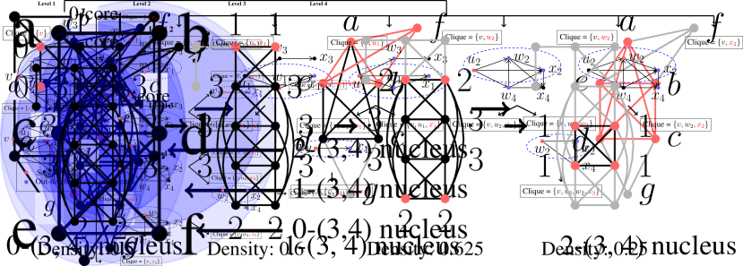
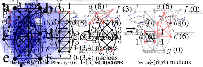
Figure 1. An example of our parallel nucleus decomposition algorithm arb-nucleus-decomp for $(r,s)=(3,4)$. At each step, we peel in parallel all triangles (3-cliques) with the minimum 4-clique count; the vertices and edges that compose of these triangles are highlighted in red. We then recompute the 4-clique count on the remaining triangles. Vertices and edges that no longer participate in any active triangles, due to previously peeled triangles, are shown in gray. Each step is labeled with the $k$-(3,4) nucleus discovered, where $k$ is the 4-clique count of the triangles highlighted in red. The figure below labels each $k$-(3,4) nucleus.

Example. An example of our algorithm for $(r,s)=(3,4)$ is shown in Figure 1. There are 14 total triangles in the example graph, namely those given by any three vertices in $\{a,b,c,d,e\}$, and the additional triangles $abf$, $bef$, $aef$, and $cdg$. At the start of the algorithm, $cdg$ is incident to no 4-cliques, while $abf$, $bef$, and $aef$ are each incident to one 4-clique. Also, $abe$ is incident to three 4-cliques, and the rest of the triangles are incident to two 4-cliques. Thus, only $cdg$ is peeled in the first round, and has a (3, 4)-clique-core number of 0. Then, $abf$, $bef$, and $aef$ are peeled simultaneously in the second round, each with a 4-clique count of one, which is also their (3, 4)-clique-core number. Peeling these triangles updates the 4-clique count of $abe$ to two, and in the third round, all remaining triangles have the same 4-clique count (and form the 2-$(3,4)$ nucleus) and are peeled simultaneously, completing the algorithm.

Figure 2. An example of the data structures in arb-nucleus-decomp during each round of $(3,4)$ nucleus decomposition, on the graph in Figure 1.

Our Algorithm. We now provide a more detailed description of the algorithm. Algorithm 2 presents the pseudocode for arb-nucleus-decomp. We refer to Figure 2, which shows the state of each data structure after each round of arb-nucleus-decomp, for an example of $(3,4)$ nucleus decomposition on the graph in Figure 1. arb-nucleus-decomp first directs the graph $G$ such that every vertex has out-degree $O(\alpha)$ (Line 20), using an efficient low out-degree orientation algorithm by Shi et al. (Shi et al., 2021a). Then, it initializes a parallel hash table $T$ to store $s$-clique counts, keyed by $r$-clique counts, and calls the recursive subroutine rec-list-cliques to count and store the number of $s$-cliques incident on each $r$-clique (Lines 21–22). It uses count-func (Lines 2–4) to atomically increment the count for each $r$-clique found in each discovered $s$-clique. As shown in Figure 2, before any rounds of peeling, $T$ contains the 4-clique count incident to each triangle. The algorithm also initializes a parallel bucketing structure $B$ that stores sets of $r$-cliques with the same $s$-clique counts (Line 23). We have four initial buckets in Figure 2. The first bucket contains $cdg$, which is incident to no $4$-cliques, and the second bucket contains $abf$, $aef$, and $bef$, which are incident to exactly one 4-clique. The third bucket contains the triangles incident to exactly two 4-cliques, $abc$, $abd$, $acd$, $ace$, $ade$, $bcd$, $bce$, $bde$, and $cde$. The final bucket contains $abe$, which is incident to exactly three 4-cliques.

1:Initialize $r$, $s$ $\triangleright$ $r$ and $s$ for $(r,s)$ nucleus decomposition

2:procedure Count-Func($T$, $S$)

3:    parfor all size $r$ subsets $R\subset S$ do

4:        Atomically add $1$ to the $s$-clique count $T[R]$     

5:procedure Update-Func($U$, $A$, $T$, $S$) ⁴

6:    Let $U^{\prime}\leftarrow\{R\subset S\mid|R|=r$ and $R\not\in A\}$

7:    Let $a$ be the # of size $r$ subsets $R\subset S$ such that $R\in A$

8:    if any $R\in U^{\prime}$ has been previously peeled then

9:        return     

10:    parfor $R$ in $U^{\prime}$ do

11:        Atomically subtract $1/a$ from the $s$-clique count $T[R]$

12:        Add $R$ to $U$     

13:procedure Update($G=(V,E),DG,A,T$)

14:    Initialize $U$ to be a parallel hash table to store $r$-cliques with updated $s$-clique counts after peeling $A$

15:    parfor $R$ in $A$ do

16:        $I\leftarrow$ intersect($N_{G}(v)$ for $v\in R$) $\triangleright$ Intersect the undirected neighbors of $v\in R$

17:        rec-list-cliques($DG$, $I$, $s-r$, $R$, update-func($U$, $A$, $T$))     

18:    return $U$

19:procedure arb-nucleus-decomp($G=(V,E)$, Orient)

20:    $DG\leftarrow$ Orient($G$) $\triangleright$ Apply a user-specified orientation algorithm

21:    Initialize $T$ to be a parallel hash table with $r$-cliques as keys, and $s$-clique counts as values

22:    rec-list-cliques($DG$, $V$, $s$, $\emptyset$, count-func($T$)) $\triangleright$ Count $s$-cliques

23:    Let $B$ be a bucketing structure mapping each $r$-clique to a bucket based on # of $s$-cliques

24:    $\mathsf{finished}\leftarrow 0$

25:    while $\mathsf{finished}<|T|$ do

26:        $A\leftarrow$ $r$-cliques in the next bucket in $B$ (to be peeled)

27:        $\mathsf{finished}\leftarrow\mathsf{finished}+|A|$

28:        $U\leftarrow$ Update$(G,DG,A,T)$ $\triangleright$ Update # of $s$-cliques and return $r$-cliques with changed $s$-clique counts

29:        Update the buckets of $r$-cliques in $U$, peeling $A$     

30:    return $B$

Algorithm 2 Parallel $(r,s)$ nucleus decomposition algorithm

While not all of the $r$-cliques have been peeled, the algorithm repeatedly obtains the $r$-cliques incident upon the lowest number of induced $s$-cliques (Line 26), updates the count of the number of peeled $r$-cliques (Line 27), and updates the $s$-clique counts of $r$-cliques that participate in $s$-cliques with peeled $r$-cliques (Line 28). In Figure 2, we see that in the first round, the bucket with the least $s$-clique count is bucket 0, and $\mathsf{finished}$ is updated to the size of the bucket, or one triangle. No 4-cliques are involved, so no updates are made to $T$, and $U$ remains empty. arb-nucleus-decomp then updates the buckets for $r$-cliques with changed $s$-clique counts (Line 29), and repeats until all $r$-cliques have been peeled. At the end, the algorithm returns the bucketing structure, which maintains the $(r,s)$-core number of each $r$-clique. In the second round in Figure 2, the bucket with the least 4-clique count is bucket 1, containing $abf$, $aef$, and $bef$. We add 3 to $\mathsf{finished}$, making its value 4. The sole 4-clique incident to these triangles is $abef$, so when these triangles are peeled, there is one fewer 4-clique incident on $abe$. Thus, the 4-clique count stored on $abe$ in $T$ is decremented by one, and $abe$ is returned in the set $U$ as the only triangle with a changed 4-clique count. Note that the (3, 4)-clique core number of $abf$, $aef$, and $bef$ is thus 1, which is implicitly maintained upon their removal from $B$. The bucket of $abe$ is updated to $2$, since $abe$ now participates in only two 4-cliques. Then, in the final round, the rest of the triangles are all in the peeled bucket, bucket 2, and the $\mathsf{finished}$ count is updated to 14, or the total number of triangles. The implicitly maintained (3, 4)-clique-core number of these triangles is 2, and since no triangles remain unpeeled, there are no further updates to the data structure and the algorithm returns.

The subroutine Update (Lines 13–18) is the main subroutine of arb-nucleus-decomp, used on Line 28. It takes as additional input the directed graph $DG$, a set $A$ of $r$-cliques to peel, and the parallel hash table $T$ that stores current $s$-clique counts, and updates incident $s$-clique counts affected by peeling the $r$-cliques in $A$. It also returns the set of $r$-cliques that have not yet been peeled with their decremented $s$-clique counts. Update first initializes a parallel hash table $U$ to store the set of $r$-cliques with changed $s$-clique counts (Line 14). It then considers each $r$-clique $R\in A$ being peeled, and computes the intersection of the undirected neighbors of the vertices in $R$, which are stored in set $I$ (Line 16). The vertices in $I$ are candidate vertices to form $s$-cliques from $R$, and Update uses $I$ with the subroutine rec-list-cliques to find the remaining $s-r$ vertices to complete the $s$-cliques incident to $R$ (Line 17). In the second round of Figure 2, $abf$, $aef$, and $bef$ are being peeled. The intersection of the neighbors of $a$, $b$, and $f$ adds vertex $e$ to the discovered 4-clique. We thus find only one 4-clique incident to $abf$, and similarly, we find the same 4-clique incident to $aef$ and $bef$.

For each $s$-clique $S$ found, rec-list-cliques calls update-func (Lines 6–12), which first checks if $S$ contains $r$-cliques that were previously peeled (Line 8). If not, update-func atomically subtracts $1/a$ from each $s$-clique count for each $r$-clique in $S$, where $a$ is the number of size $r$ subsets in $S$ that are also being peeled (Line 11). This is to prevent over-counting—if $r$-cliques that participate in the same $s$-clique are peeled simultaneously, then they will each subtract $1/a$ from the $s$-clique count, and the total subtraction will sum to $1$ for this $s$-clique. update-func also adds each $r$-clique with updated counts to $U$ (Line 12). In the second round of Figure 2, since $abf$, $aef$, and $bef$ each discover the 4-clique $abef$, which consists of $a=3$ triangles that are simultaneously being peeled, $abf$, $aef$, and $bef$ each decrement $1/3$ from the 4-clique count of $abe$ in $T$. In total, $1$ is decremented from $abe$’s 4-clique count. Then, $abe$ is added to $U$, since its 4-clique count has been updated. In the third round, because all remaining triangles are being peeled in $A$, the set $U^{\prime}$ defined on Line 6, is either empty or contains a previously peeled triangle, by definition. Thus, Update returns without performing any modifications to $U$ or $T$, and no buckets are updated. Afterwards, the $\mathsf{finished}$ variable equals the total number of triangles, and the algorithm finishes.

We now discuss the theoretical efficiency our parallel nucleus decomposition algorithm. To show that our algorithm improves upon the best existing work bounds for the sequential nucleus decomposition algorithm, we use the following key lemma that upper bounds the sum of the minimum degrees of vertices over all $c$-cliques. We note that Chiba and Nishizeki (Chiba and Nishizeki, 1985) first proved this lemma for $c=2$, and Eden et al. first proved this lemma for larger $c$ (Eden et al., 2020). We provide a similar proof here.

Lemma 4.1 ((Eden et al., 2020)).

For a graph $G$ with arboricity $\alpha$, over all $c$-cliques $C_{c}=\allowbreak\{v_{1},\ldots,v_{c}\}$ in $G$ where $c\geq 1$, $\sum_{C_{c}}\min_{1\leq i\leq c}\text{deg}(v_{i})=O(m\alpha^{c-1})$.

• First, the $c=1$ case is easy, since $\sum_{v_{i}\in V}\text{deg}(v_{i})=2m$, and the $c=2$ case is proven by Chiba and Nishizeki (Chiba and Nishizeki, 1985). We consider $c\geq 3$ for the rest of the proof.

We begin by rewriting the sum $\sum_{C_{c}}\min_{1\leq i\leq c}\text{deg}(v_{i})$ to be taken over all edges $e\in E$ instead of over all $c$-cliques $C_{c}$. Importantly, we must assign each unique $c$-clique $C_{c}$ to a unique edge $e$ contained within $C_{c}$, to avoid double counting. We perform this assignment using an $O(\alpha)$-orientation of the graph, where each $c$-clique $C_{c}$ is an ordered list of vertices $v_{i}$ for $1\leq i\leq c$, with the ordering given by the $O(\alpha)$-orientation. We assign each $C_{c}$ to the edge $e$ given by its first two vertices $v_{1}$ and $v_{2}$.

Then, rewriting the sum $\sum_{C_{c}}\min_{1\leq i\leq c}\text{deg}(v_{i})$ to be taken over all edges, we obtain $\sum_{e\in E}\sum_{C_{c}\text{ assigned to }e}\min_{1\leq i\leq c}\text{deg}(v_{i})$. For each edge $e$, the quantity inside the inner sum is upper bounded by the minimum of the degrees of the endpoints of $e$, so we have $\sum_{e=(u,v)\in E}\min(\text{deg}(u),\allowbreak\text{deg}(v))\cdot($# of $C_{c}$ assigned to $e)$.

We now claim that the number of $c$-cliques $C_{c}$ assigned to each edge $e=(u,v)$ is upper bounded by $O(\alpha^{c-2})$. This fact follows by virtue of the $O(\alpha)$-orientation used earlier to assign $c$-cliques $C_{c}$ to edges. Namely, if we let $DG$ denote the directed graph given by the $O(\alpha)$-orientation, then by construction for each $C_{c}$, vertices $v_{i}\in C_{c}$ for $i>2$ must be out-neighbors of $v_{1}$ and $v_{2}$. There are at most $O(\alpha)$ out-neighbors in the intersection of $N_{DG}(u)$ and $N_{DG}(v)$ that could potentially complete a directed $c$-clique with the vertices $u$ and $v$. With $c-2$ additional vertices necessary to complete a directed $c$-clique, and $O(\alpha)$ vertices to choose from, there are at most $O(\alpha^{c-2})$ such directed $c$-cliques.

Thus, our desired sum is given by $\sum_{e=(u,v)\in E}\min(\text{deg}(u),\allowbreak\text{deg}(v))\cdot($# of $C_{c}$ assigned to $e)=\allowbreak O(\alpha^{c-2}\sum_{e=(u,v)\in E}\min(\text{deg}(u),\allowbreak\text{deg}(v)))$. By Lemma 2 of (Chiba and Nishizeki, 1985), we know that $\sum_{e=(u,v)\in E}\min(\text{deg}(u),\text{deg}(v))=\allowbreak O(m\alpha)$. Therefore, in total, we have $\sum_{C_{c}}\min_{1\leq i\leq c}\text{deg}(v_{i})=\allowbreak O(m\alpha^{c-1})$, as desired. ∎

Using this key lemma, we prove the following complexity bounds for our parallel nucleus decomposition algorithm. $\rho_{(r,s)}(G)$ is defined to be the $\bm{(r,s)}$ peeling complexity of $G$, or the number of rounds needed to peel the graph where in each round, all $r$-cliques with the minimum $s$-clique count are peeled. $\rho_{(r,s)}(G)\leq O(m\alpha^{r-2})$, since at least one $r$-clique is peeled in each round.

Theorem 4.2.

arb-nucleus-decomp computes the $(r,s)$ nucleus decomposition in $O(m\alpha^{s-2}+\rho_{(r,s)}(G)\log n)$ amortized expected work and $O(\rho_{(r,s)}(G)\log n+\log^{2}n)$ span w.h.p., where $\rho_{(r,s)}(G)$ is the $(r,s)$ peeling complexity of $G$.

• First, the work and span of counting the number of $s$-cliques per $r$-clique is given directly by Shi et al. (Shi et al., 2021a), since we use this $s$-clique enumeration algorithm, rec-list-cliques, as a subroutine. Because we hash each $s$-clique count per $r$-clique in parallel, this takes $O(m\alpha^{s-2})$ work and $O(\log^{2}n)$ span w.h.p. for a constant $s$.

  We now discuss the work and span of obtaining the set of $r$-cliques with minimum $s$-clique count and updating the $s$-clique counts in our bucketing structure $B$. We make use of the fact that the total number of $c$-cliques in $G$ is bounded by $O(m\alpha^{c-2})$, which follows from the $c$-clique enumeration algorithm (Shi et al., 2021a). The overall work of inserting $r$-cliques into $B$ is given by the number of $r$-cliques in $G$, or $O(m\alpha^{r-2})$. Each $r$-clique has its bucket decremented at most once per incident $s$-clique, and because there are at most $O(m\alpha^{s-2})$ $s$-cliques, the work of updating buckets is given by $O(m\alpha^{s-2})$. Finally, extracting the minimum bucket can be done in $O(\log n)$ amortized expected work and $O(\log n)$ span w.h.p., which in total gives $O(\rho_{(r,s)}(G)\log n)$ amortized expected work, and $O(\rho_{(r,s)}(G)\log n)$ span w.h.p.

  Finally, it remains to discuss the work and span of obtaining updated $s$-clique counts after peeling each set of $r$-cliques, or the work and span of the Update subroutine. For each $r$-clique $R$, Update first computes the intersection of the neighbors of each vertex $v\in R$, and stores them in set $I$. Notably, the total work of intersecting the neighbors of each vertex $v\in R$ over all $r$-cliques $R$ is given by $O(\sum_{R}\min_{1\leq i\leq r}\text{deg}(v_{i}))=O(m\alpha^{r-1})$ w.h.p., which follows from Lemma 4.1, and the span across all intersections is $O(\log n)$ w.h.p. for a constant $r$.

Update then calls the rec-list-cliques subroutine to complete $s$-cliques from $R$, taking as input the sets $I$ computed in the previous step. Each successive recursive call to rec-list-cliques takes a multiplicative $O(\alpha)$ work w.h.p. due to the intersection operation, and rec-list-cliques requires $s-r$ recursive levels to complete each $s$-clique. This results in a total multiplicative factor of $O(\alpha^{s-r-1})$ work w.h.p., because the final recursive level (as shown in the $r\ell=1$ case in rec-list-cliques) does not involve any intersection operations, and simply iterates through the discovered $s$-cliques. Thus, including the initial cost of setting up the call to rec-list-cliques, and using the fact that the number of potential neighbors in the sets $I$ across all $r$-cliques is $O(m\alpha^{r-1})$, the total work of rec-list-cliques across all $r$-cliques is given by $O(m\alpha^{r-1}\cdot\alpha^{s-r-1})=\allowbreak O(m\alpha^{s-2})$ w.h.p. The span of each intersection on each recursive level is $O(\log n)$ w.h.p., and there are $\rho_{(r,s)}(G)$ rounds by definition, which contributes $O(\rho_{(r,s)}(G)\log n)$ overall. ∎

Discussion. arb-nucleus-decomp is work-efficient with respect to the best sequential algorithm, and improves upon the best sequential algorithm that uses sublinear space in the number of $s$-cliques. In more detail, the previous best sequential bounds were given by Sariyüce et al. (Sariyüce et al., 2017), in terms of the number of $c$-cliques containing each vertex $v$, or $ct_{c}(v)$, and the work of an arbitrary $c$-clique enumeration algorithm, or $RT_{c}$. Assuming space proportional to the number of $s$-cliques and the number of $r$-cliques in the graph, they compute the $(r,s)$ nucleus decomposition in $O(RT_{r}+RT_{s})=O(RT_{s})$ work, and assuming space proportional to only the number of $r$-cliques in the graph, they compute the $(r,s)$ nucleus decomposition in $O(RT_{r}+\sum_{v\in V(G)}ct_{r}(v)\cdot\text{deg}(v)^{s-r})$ work. We discuss these bounds in detail and provide a comparison to arb-nucleus-decomp in the appendix. Specifically, arb-nucleus-decomp uses space proportional to the number of $r$-cliques due to the space required for $T$ and $B$, and is work-efficient with respect to the best sequential algorithm that uses the same space, improving upon the corresponding bound given by Sariyüce et al. (Sariyüce et al., 2017). If more space is permitted, a small modification of our algorithm yields a sequential nucleus decomposition algorithm that performs $O(m\alpha^{s-2})$ work, matching the corresponding bound given by Sariyüce et al. (Sariyüce et al., 2017). The idea is to use a dense bucketing structure with space proportional to the total number of $s$-cliques, since finding the next bucket with the minimum $s$-clique count involves a simple linear search rather than a heap operation. In the parallel setting, arb-nucleus-decomp can work-efficiently find the minimum non-empty bucket by performing a series of steps, where at each step $i$, arb-nucleus-decomp searches in parallel the region $[2^{i},2^{i+1}]$ for the next non-empty bucket. This search procedure takes logarithmic span, and is work-efficient with respect to the sequential algorithm.

5. Practical Optimizations

We now introduce the practical optimizations that we use for our parallel $(r,s)$ nucleus decomposition implementation.

5.1. Number of Parallel Hash Table Levels

arb-nucleus-decomp uses a single parallel hash table $T$ to store the $s$-clique counts, where the keys are $r$-cliques. However, this storage method is infeasible in practice due to space limitations, particularly for large $r$, since $r$ vertices must be concatenated into a key for each $r$-clique. We observe that space can be saved by introducing more levels to our parallel hash table $T$. For example, one option is to instead use a two-level combination of an array and a parallel hash table, which consists of an array of size $n$ whose elements are pointers to individual hash tables where the keys are $(r-1)$-cliques. The $s$-clique count for a corresponding $r$-clique $R=\{v_{1},\ldots,v_{r}\}$ (where the vertices are in sorted order) is stored by indexing into the $v_{1}^{\text{th}}$ element of the array, and storing the count on the key corresponding to the $(r-1)$-clique given by $\{v_{2},\ldots,v_{r}\}$ in the given hash table. Space savings arise because $v_{1}$ does not have to be repeatedly stored for each $(r-1)$-clique in its corresponding hash table, but rather is only stored once in the array.

A more general option, particularly for large $r$, is to use a multi-level parallel hash table, with $\ell\leq r$ levels in which each intermediate level consists of a parallel hash table keyed by a single vertex in the $r$-clique whose value is a pointer to a parallel hash table in the subsequent level, and the last level consists of a parallel hash table keyed by $(r-\ell+1)$-cliques. Given an $r$-clique $R=\{v_{1},\ldots,v_{r}\}$ (where the vertices are in sorted order), each of the vertices in the clique in order is mapped to each level of the hash table, except for the last $(r-\ell+1)$ vertices which are concatenated into a key for the last level of the hash table. Thus, the location in the hash table corresponding to $R$ can be found by looking up the key $v_{j}$ in the hash table at each level for $j<\ell$, and following the pointer to the next level. At the last level, the key is given by the $(r-\ell+1)$-clique corresponding to $\{v_{\ell},\ldots,v_{r}\}$. Again, space savings arise due to the shared vertices on each intermediate level, which need not be repeatedly stored in the keys on the subsequent levels of the parallel hash table, and for $r\geq\ell>2$, these savings may exceed those found in the previous combination of an array and a parallel hash table.

In considering different numbers of levels, we differentiate between the two-level combination of an array and a parallel hash table, and the $\ell$-multi-level option of nested parallel hash tables, where $\ell$ is the number of levels, and notably, we may have $\ell=2$. Figures 3 and 4 show examples of $T$ using different numbers of levels. As shown in these examples, there are cases where increasing the number of levels does not save space, because the additional pointers required in increasing the number of levels exceeds the overlap in vertices between $r$-cliques, particularly for small $r$.

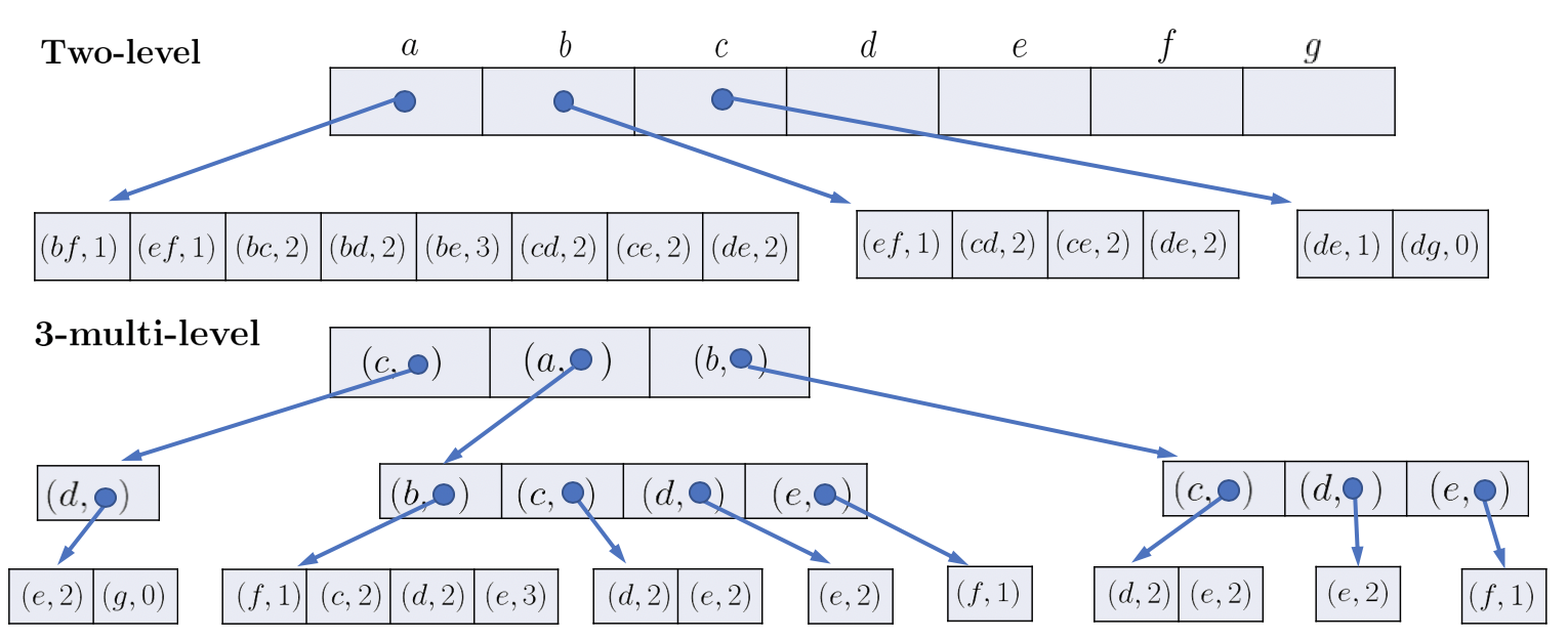
Figure 3. An example of the initial parallel hash table $T$ for $(3,4)$ nucleus decomposition on the graph from Figure 1, considering different numbers of levels. Note that Figure 2 shows a one-level parallel hash table $T$. If we consider each vertex and each pointer to take a unit of memory, the one-level $T$ takes 42 units, while the two-level $T$ takes 35 units, thus saving memory. However, the 3-multi-level $T$ takes 50 units, because $r=3$ is too small to give memory savings for this graph.

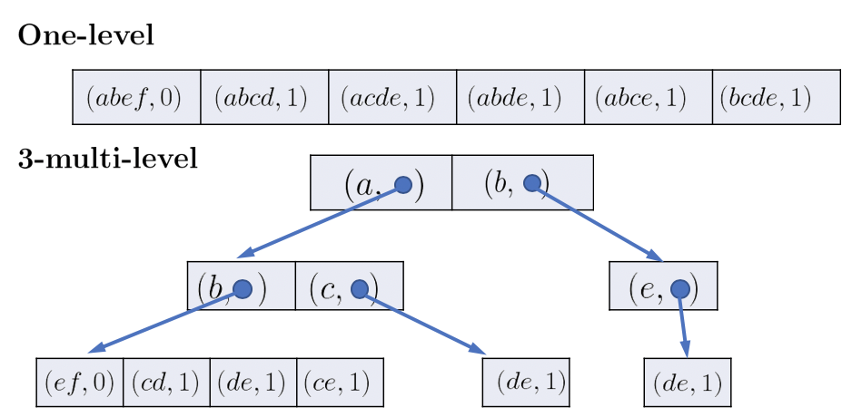
Figure 4. An example of the initial parallel hash table $T$ for $(4,5)$ nucleus decomposition on the graph from Figure 1, considering different numbers of levels. If we consider each vertex and each pointer to take a unit of memory, the one-level $T$ takes 24 units, while the 3-multi-level $T$ takes 22 units, thus saving memory. We see memory savings with more levels in $T$ compared to in Figure 3, because $r=4$ is sufficiently large.

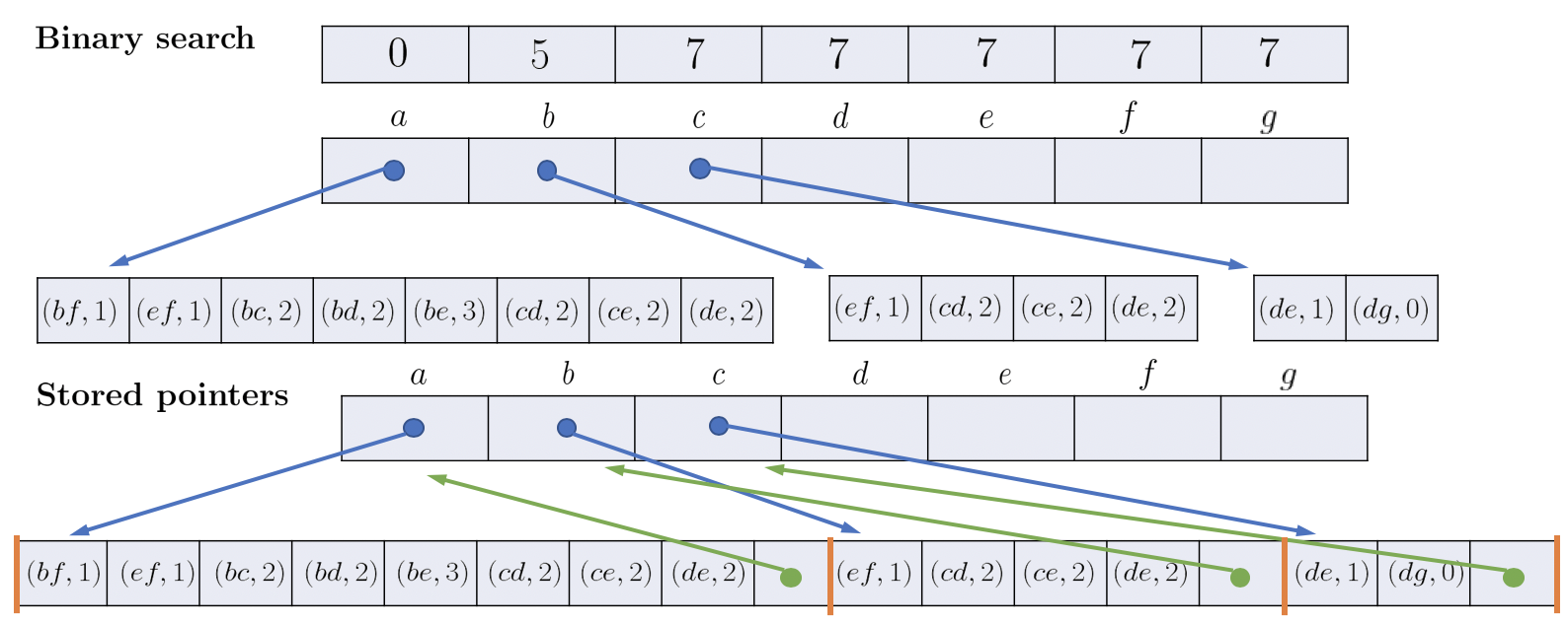
Figure 5. Using the same graph as shown in Figure 1 and the two-level $T$ from Figure 3, for $(3,4)$ nucleus decomposition, an example of the binary search and stored pointers methods.

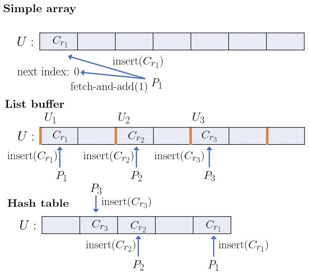
Figure 6. An example of the simple array, list buffer, and hash table options in aggregating the set $U$ of $r$-cliques with updated $s$-clique counts. Processors $P_{1}$, $P_{2}$, and $P_{3}$ are storing $r$-cliques $C_{r_{1}}$, $C_{r_{2}}$, and $C_{r_{3}}$, respectively, in $U$.

Moreover, note that there are no theoretical guarantees on whether additional levels will result in a memory reduction, since a memory reduction depends on the number of overlapping $r$-cliques and the size of the overlap in $r$-cliques in any given graph. In other words, the skew in the constituent vertices of the $r$-cliques directly impacts the possible memory reduction. Similarly, performance improvements may arise due to better cache locality in accessing $r$-cliques that share many vertices, but this is not guaranteed, and cache misses are inevitable while traversing through different levels.

The idea of a multi-level parallel hash table is more generally applicable in scenarios where the efficient storage and access of sets with significant overlap is desired, particularly if memory usage is a bottleneck. An example use case is to efficiently store the hyperedge adjacency lists for a hypergraph. The multi-level parallel hash table can also be used for data with multiple fields or dimensions, where each level keys a different field.

5.2. Contiguous Space

In using the two-level and multilevel data structures as $T$, a natural way to implement the last level parallel hash tables in these more complicated data structures is to simply allocate separate blocks of memory as needed for each last level parallel hash table. However, this approach may be memory-inefficient and lead to poor cache locality. An optimization for the two-level and multi-level tables is to instead first compute the space needed for all last level parallel hash tables and then allocate a contiguous block of memory such that the last level tables are placed consecutively with one another, using a parallel prefix sum to determine each of their indices into the contiguous block of memory. This optimization requires little overhead, and has the additional benefit of greater cache locality. This optimization does not apply to one-level parallel hash tables, since they are by nature contiguous.

5.3. Binary Search vs. Stored Pointers

An important implementation detail from arb-nucleus-decomp is the interfacing between the representation of $r$-cliques in the bucketing structure $B$ and the representation of $r$-cliques in the parallel hash table $T$. It is impractical to use the theoretically-efficient Fibonacci heap used to obtain our theoretical bounds, due to the complexity of Fibonacci heaps in general; in practice, we use the efficient parallel bucketing implementation by Dhulipala et al. (Dhulipala et al., 2017).

This bucketing structure requires each $r$-clique to be represented by an index, and to interface between $T$ and $B$, we require a map translating each $r$-clique in $T$ to its index in $B$, and vice versa. More explicitly, for a given $r$-clique in $T$, we must be able to find the number of $s$-cliques it participates in using $B$, and symmetrically, for a given $r$-clique that we peel from $B$, we must be able to find its constituent vertices using $T$. It would be impractical in terms of space to represent the $r$-clique directly using its constituent vertices in $B$, since its constituent vertices are already stored in $T$. Thus, we seek a unique index to represent each $r$-clique by in $B$, that is easy to map to and from the $r$-clique in $T$. If $T$ is represented using a one-level parallel hash table, then a natural index to use for each $r$-clique is its key in $T$, and the map is implicitly the identity map. For instance, considering the one-level $T$ in Figure 2, instead of storing $cdg$ in bucket 0 before any rounds begin, we would instead store 13, which is the index of $cdg$ in $T$. However, if $T$ is represented using a two-level or multi-level structure, then the index representation and map are less natural, and require additional overheads to maintain.

One important property of the mapping from $T$ to $B$ is space-efficiency, and so it is desirable to maintain an implicit map. Therefore, we represent each $r$-clique by the unique index corresponding to its position in the last level parallel hash table in $T$, which can be implicitly obtained by its location in memory if $T$ is represented contiguously. If $T$ is not represented contiguously, then we can store the prefix sums of the sizes of each successive level of parallel hash tables, and use these plus the $r$-clique’s index at its last level table in $T$ to obtain the unique index. For equivalent $T$, the index corresponding to each $r$-clique is the same regardless of whether $T$ is represented contiguously in memory or not. For instance, considering the two-level $T$ in Figure 3, instead of storing $abc$ in bucket 2 before any rounds begin, we would instead store 2, which is the index of $abc$ in the second level of $T$. Similarly, instead of storing $bef$ in bucket 1, we would instead store 8; this is because we take the index corresponding to $bef$ to be its index in the second level hash table corresponding to vertex $b$, plus the sizes of earlier second level hash tables, namely the size of the hash table corresponding to vertex $a$. Then, it is also necessary to implicitly maintain the inverse map, from an index in $B$ to the constituent vertices of the corresponding $r$-clique, for which we provide two methods.

Binary Search Method. One solution is to store the prefix sums of the sizes of each successive level of parallel hash tables in both the contiguous and non-contiguous cases, and use a serial binary search to find the table corresponding to the given index at each level. We also store the vertex corresponding to each intermediate level alongside each table, which can be easily accessed after the binary search. The key at the last level table can then be translated to its constituent $r-\ell$ vertices. This does not require the last level parallel hash tables to be stored contiguously in memory. Figure 5 shows an example of this method in the non-contiguous case, where the top array is the prefix sum of the sizes of the second level hash tables. Each entry in the prefix sum corresponds to an entry in the first level, which contains the first vertex of the triangle and points to the second level, which contains the other two vertices.

Stored Pointer Method. However, while using binary searches is a natural solution, they may be computationally inefficient, both in terms of work and cache misses, considering the number of such translations that are needed throughout arb-nucleus-decomp. Instead, we consider a more sophisticated solution which, assuming contiguous memory, is to place barriers between parallel hash tables on each level that contain up-pointers to prior levels, and fill empty cells of the parallel hash tables with the same up-pointers. Then, given an index to the last level, which translates directly into the memory location of the cell containing the last level $r$-clique key due to the contiguous memory, we can perform linear searches to the right until it reaches an empty cell, which directly gives an up-pointer to the prior level (and thus, also the vertex corresponding to the prior level). We differentiate between empty and non-empty cells by reserving the top bit of each key to indicate whether the cell is empty or non-empty. The benefit of this method is that with a good hashing scheme, the linear search for an empty cell will be faster and more cache-friendly compared to a full binary search. Figure 5 also shows an example of this method using contiguous space, in which the barriers placed to the right of each hash table in the second level point back to the parent entry in the first level, allowing an index to traverse up these pointers to obtain the corresponding first vertex of the triangle. Note that the bold orange lines on the second level mark the boundaries between parallel hash tables corresponding to different vertices from the first level.

With both the contiguous space and stored pointers optimizations applied to two-level and multi-level parallel hash tables $T$, we show in Section 6.2 that we achieve up to a 1.32x speedup of using a two-level $T$, and up to a 1.46x speedup of using an $\ell$-multi-level $T$ for $\ell>2$, over one level.

5.4. Graph Relabeling

We sort the vertices in each $r$-clique prior to translating it into a unique key for use in the parallel hash table $T$. However, the lexicographic ordering of vertices in the input graph may not be representative of the access patterns used in finding $r$-cliques. In particular, because we use directed edges based on an $O(\alpha)$-orientation to count $r$-cliques and $s$-cliques, an optimization that could save work and improve cache locality in accessing $T$ is to relabel vertices based on the $O(\alpha)$-orientation, so that the sorted order is representative of the order in which vertices are discovered in the rec-list-cliques subroutine. The first benefit of this optimization is that there is no need to re-sort $r$-cliques based on the orientation, which is implicitly performed on Line 4 of Algorithm 2, as after relabeling, the vertices in a clique will be added in increasing order. A second benefit is that $r$-cliques discovered in the same recursive hierarchy will be located closer together in our parallel hash table, potentially leading to better cache locality when accessing their counts in $T$. In our evaluation in Section 6.2, we see up to a 1.29x speedup using graph relabeling.

5.5. Obtaining the Set of Updated $r$-cliques

A key component of the bucketing structure in arb-nucleus-decomp is the computation of the set $U$ of $r$-cliques with updated $s$-clique counts, after peeling a set of $r$-cliques. Using a parallel hash table with size equal to the number of $r$-cliques is slow in practice due to the need to iterate through the entire hash table to retrieve the $r$-cliques and to clear the hash table. We present here three options for computing $U$. Figure 6 shows an example of each of these.

Simple Array. The first option is to represent $U$ as a simple array to hold $r$-cliques, along with a variable that maintains the next open slot in the array. We use a fetch-and-add to update the $s$-clique count of a discovered $r$-clique in the Update-Func subroutine, and if in the current round this is the first such modification of the $r$-clique’s count, we use a fetch-and-add to reserve a slot in $U$, and store the $r$-clique in the reserved slot in $U$. This method introduces contention due to the requirement of all updated $r$-cliques to perform a fetch-and-add with a single variable to reserve a slot in $U$. As shown in Figure 6, processor $P_{1}$ successfully updates the index variable and inserts its $r$-clique $C_{r_{1}}$ into the first index in $U$, but the other processors must wait until their fetch-and-add operations succeed. However, the $r$-cliques are compactly stored in $U$ and there is no need to clear elements in $U$, which results in time savings.

List Buffer. The second option improves upon the contention incurred by the first option, offering better performance. We use a data structure that we call a list buffer, which consists of an array $U$ that holds $r$-cliques, and $P$ variables $\{i_{1},\ldots,i_{P}\}$ that maintain the next open slots in the array, where $P$ is the number of threads. Each of the $P$ variables is exclusively assigned to one of the $P$ threads. The data structure also uses a constant buffer size, and each thread is initially assigned a contiguous block of $U$ of size equal to this constant buffer size. When a thread $j$ is the first to modify an $r$-clique’s count in a given round, the thread updates its corresponding $i_{j}$, and uses the reserved open slot in $U$ to store the $r$-clique. If a thread runs out of space in its assigned block in $U$, it uses a fetch-and-add operation to reserve the next available block in $U$ of size equal to the constant buffer size. We filter $U$ of all unused slots, prior to returning $U$ to the bucketing data structure. The reduced contention is due to the exclusive $i_{j}$ that each thread $j$ can update without contention. Threads may still contend on reserving new blocks of space in $U$, but the contention is minimal with a large enough buffer size. In reusing the list buffer data structure in later rounds, there is no need to clear $U$, as it is sufficient to reset the $i_{j}$. In Figure 6, the buffer size is 2, and the slots in $U$ assigned to each processor $P_{i}$ are labeled by $U_{i}$. Each $P_{i}$ can store its corresponding $r$-clique $C_{r_{i}}$ in parallel, since there is no contention within their buffer as long as the buffer is not full.

Hash Table. The last option reduces potential contention even further by removing the necessity to reserve space, but at the cost of additional work needed to clear $U$ between rounds. This option uses a parallel hash table as $U$, but dynamically determines the amount of space required on each round based on the number of $r$-cliques peeled, and as such, the maximum possible number of $r$-cliques with updated $s$-clique counts. Thus, in rounds with fewer $r$-cliques peeled, less space is reserved for $U$ for that round, and as a result, less work is required to clear the space to reuse in the next round. Figure 6 shows each processor $P_{i}$ storing its corresponding $r$-clique $C_{r_{i}}$ into the parallel hash table. However, the entirety of $U$ must be cleared in order to reuse $U$ between rounds.

In our evaluation in Section 6.2, we achieve up to a 3.98x speedup using a list buffer and up to a 4.12x speedup using a parallel hash table, both over a simple array.

5.6. Graph Contraction

In the special case of $(2,3)$ nucleus (truss) decomposition, we introduce an optimization that filters out peeled edges when a significant number of edges have been peeled over successive rounds. When many edges have been peeled, reducing the overall size of the graph and contracting adjacency lists may save work in future rounds, in that work does not need to be spent iterating over previously peeled edges, allowing for performance improvements.

We perform this contraction when the number of peeled edges since the previous contraction is at least twice the number of vertices in the graph, and we only contract adjacency lists of vertices that have lost at least a quarter of their neighbors since the previous contraction. We chose these boundaries for contraction heuristically based on performance on real-world graphs; these generally allow for contraction to be performed only in instances in which it could meaningfully impact the performance of future operations. Specifically, we found that the overhead of each contraction operation is balanced by reduced work in future iterations only when vertices can significantly reduce the size of their adjacency lists, and iterating through vertices to check for this condition is only worthwhile when sufficiently many edges have been peeled. Note that the $k$-truss decomposition implementation by Che et al. (Che et al., 2020) also periodically contracts the graph. In terms of implementation details, the contraction operations are performed in parallel for each vertex. If a vertex meets the heuristic criteria, its adjacency list is filtered into a new adjacency list sans the peeled edges, using the parallel filter primitive; this new adjacency list replaces the previous adjacency list. This optimization does not extend to higher $(r,s)$ nucleus decomposition, because if an $r$-clique has been peeled for $r>2$, its edges may still be involved in other unpeeled $r$-cliques. Thus, there is no natural way to contract out an $r$-clique from a graph for $r>2$ to allow for work savings in future rounds. In Section 6.2, we see up to a 1.08x speedup using graph contraction in $(2,3)$ nucleus decomposition.

6. Evaluation

6.1. Environment and Graph Inputs

We run experiments on a Google Cloud Platform instance of a 30-core machine with two-way hyper-threading, with 3.8 GHz Intel Xeon Scalable (Cascade Lake) processors and 240 GiB of main memory. We compile with g++ (version 7.4.0) and use the -O3 flag. We use the work-stealing scheduler ParlayLib by Blelloch et al. (Blelloch et al., 2020). We terminate any experiment that takes over 6 hours. We test our algorithms on real-world graphs from the Stanford Network Analysis Project (SNAP) (Leskovec and Krevl, 2019), shown in Figure 7 with $\rho_{(r,s)}$ and the maximum $(r,s)$-core numbers for $r<s\leq 7$. We also use synthetic rMAT graphs (Chakrabarti et al., 2004), with $a=0.5$, $b=c=0.1$, and $d=0.3$.

We compare to Sariyüce et al.’s state-of-the-art parallel (Sariyüce et al., 2018) and serial (Sariyüce et al., 2017) nucleus decomposition implementations, which address $(2,3)$ and $(3,4)$ nucleus decomposition. For the special case of $(2,3)$ nucleus decomposition, we compare to Che et al.’s (Che et al., 2020) highly optimized state-of-the-art parallel pkt-opt-cpu, and implementations by Kabir and Madduri’s pkt (Kabir and Madduri, 2017b), Smith et al.’s msp (Smith et al., 2017), and Blanco et al. (Blanco et al., 2019), which represent the top-performing implementations from the MIT GraphChallenge (GraphChallenge, 2021). We run all of these using the same environment as our experiments on arb-nucleus-decomp.

6.2. Tuning Optimizations

There are six total optimizations that we implement in arb-nucleus-decomp: different numbers of levels in our parallel hash table $T$ (numbers of levels), the use of contiguous space (contiguous space), a binary search versus stored pointers to perform the mapping of indices representing $r$-cliques to the constituent vertices (inverse index map), graph relabeling (graph relabeling), a simple array method versus a list buffer versus a parallel hash table for maintaining the set $U$ of $r$-cliques with changed $s$-clique counts per round (update aggregation), and graph contraction specifically for $(2,3)$ nucleus decomposition (graph contraction).

	$n$	$m$
amazon	334,863	925,872
dblp	317,080	1,049,866
youtube	1,134,890	2,987,624
skitter	1,696,415	11,095,298
livejournal.	3,997,962	34,681,189
orkut	3,072,441	117,185,083
friendster	65,608,366	$1.806\times 10^{9}$

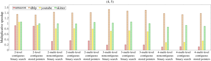
Figure 7. Sizes of our input graphs, all of which are from (Leskovec and Krevl, 2019), on the left, and the number of rounds required $\rho_{(r,s)}$ and the maximum $(r,s)$-core numbers for $r<s\leq 7$ for each graph on the right.

Figure 8. On the left, multiplicative speedups of different combinations of optimizations on $T$ in arb-nucleus-decomp, over an unoptimized setting of arb-nucleus-decomp, for $(3,4)$ nucleus decomposition. On the right, multiplicative space savings for $T$ of different combinations of optimizations on $T$ in arb-nucleus-decomp, over the unoptimized setting, for $(3,4)$ nucleus decomposition. Note that the space usage between the non-contiguous option and the contiguous option is equal. Friendster is omitted because arb-nucleus-decomp runs out of memory for this graph.

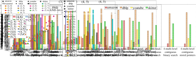
Figure 9. Multiplicative speedups of different combinations of optimizations on $T$ in arb-nucleus-decomp, over an unoptimized setting of arb-nucleus-decomp, for $(4,5)$ nucleus decomposition. Livejournal, orkut, and friendster are omitted, because arb-nucleus-decomp runs out of memory for these instances.

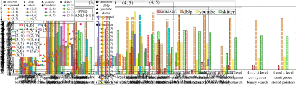
Figure 10. Multiplicative space savings for $T$ of different combinations of optimizations on $T$ in arb-nucleus-decomp, over the unoptimized setting, for $(4,5)$ nucleus decomposition. Note that the space usage between the non-contiguous option and the contiguous option is equal. Also, livejournal, orkut, and friendster are omitted, because arb-nucleus-decomp runs out of memory for these instances.

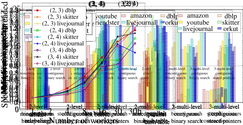
Figure 11. Multiplicative speedups of the graph relabeling, update aggregation, and graph contraction optimizations in arb-nucleus-decomp, over a two-level setting with contiguous space and stored pointers, and using the simple array for $U$. Friendster is omitted from the $(2,4)$ and $(3,4)$ nucleus decomposition experiments, because the unoptimized arb-nucleus-decomp times out for $(2,4)$, and arb-nucleus-decomp runs out of memory for $(3,4)$.

The most unoptimized form of arb-nucleus-decomp uses a one-level parallel hash table $T$, no graph relabeling, and the simple array method for the update aggregation (as this is the simplest and most intuitive method), and in the case of $(2,3)$ nucleus decomposition, no graph contraction. Note that the contiguous space and inverse index map optimizations do not apply to the one-level $T$.

Because the first three optimizations, namely numbers of levels, contiguous space, and the inverse index map, apply specifically to the parallel hash table $T$, while the remaining optimizations apply generally to the rest of the nucleus decomposition algorithm, we first tune different combinations of options for the first three optimizations against the unoptimized arb-nucleus-decomp. We then separately tune the remaining optimizations, namely graph relabeling, update aggregation, and graph contraction optimizations, against both the unoptimized arb-nucleus-decomp and the best choice of optimizations from the first comparison.

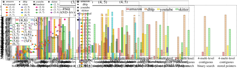
Figure 12. Multiplicative slowdowns over our parallel arb-nucleus-decomp of pkt-opt-cpu and pkt for $(2,3)$ nucleus decomposition, and of single-threaded arb-nucleus-decomp, pnd, and, and-nn, and nd for $(2,3)$ and $(3,4)$ nucleus decomposition. The label arb-nucleus-decomp in the legend refers to our single-threaded running times. We have omitted bars for pnd, and, and-nn, and nd where these implementations run out of memory or time out. We have included in parentheses the times of our parallel arb-nucleus-decomp on 30 cores with hyper-threading. We have also included a line marking a multiplicative slowdown of 1 for $r=2$, $s=3$, and we see that pkt-opt-cpu outperforms arb-nucleus-decomp on skitter, livejournal, orkut, and friendster.

Figure 13. Multiplicative slowdowns of parallel arb-nucleus-decomp for each $(r,s)$ combination over the fastest running time for parallel arb-nucleus-decomp across all $r<s\leq 7$ for each graph (excluding $(2,3)$ and $(3,4)$, which are shown in Figure 12). The fastest running time is labeled in parentheses below each graph. Also, livejournal is excluded because for these $r$ and $s$, arb-nucleus-decomp is only able to complete $(2,4)$ nucleus decomposition, in 484.74 seconds, and the rest timed out. We have omitted bars where arb-nucleus-decomp runs out of memory or times out.

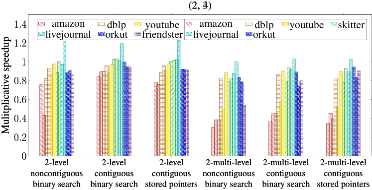
Figure 14. Speedup of arb-nucleus-decomp over its single-threaded running times. ”30h” denotes 30-cores with two-way hyper-threading.

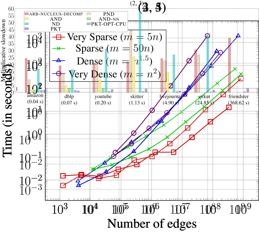
Figure 15. Running times of parallel arb-nucleus-decomp on rMAT graphs of varying densities for $(2,3)$, $(3,4)$, and $(4,5)$ nucleus decomposition. We remove duplicate generated edges.

Optimizations on $T$. Across $(2,3)$, $(2,4)$, $(3,4)$, and $(4,5)$ nucleus decomposition, using a two-level $T$ with contiguous space and stored pointers for the inverse index map gives the overall best configuration across these $r$ and $s$ values, with up to 1.32x speedups over the unoptimized case. This configuration either outperforms or offers comparable performance to other configurations. Figure 8 and 9 shows the multiplicative speedup of each combination of optimizations on $T$ over the unoptimized $T$ for $(3,4)$ nucleus decomposition and $(4,5)$ nucleus decomposition, respectively; friendster is omitted from our $(3,4)$ experiments because arb-nucleus-decomp runs out of memory on these graphs. Also, the speedups for $(2,3)$ and $(2,4)$ nucleus decomposition are omitted, but show similar behavior overall.

On the smallest graph, amazon, we see universally poor performance of the two-level and multi-level options, and the one-level $T$ outperforms these options; however, we note that the one-level running times for arb-nucleus-decomp on amazon in these cases is $<0.2$ seconds and the maximum core number of amazon is particularly small ($\leq 10$), and so the optimizations simply add too much overhead to see performance improvements. The main case where the two-level $T$ performs noticeably worse than other options is for large graphs and for large $r$ and $s$. In $(3,4)$ nucleus decomposition, we note that for orkut, using a $3$-multi-level $T$, also with contiguous space and stored pointers, significantly outperforms the analogous two-level option, with a 1.34x speedup over the unoptimized case compared to a 1.11x speedup. Similarly, in $(4,5)$ nucleus decomposition, using a 3-multi-level $T$ offers comparable performance to the two-level $T$ on dblp and skitter (the 3-multi-level $T$ gives 1.46x and 1.06x speedups over the unoptimized $T$, respectively, while the 2-level $T$ gives 1.32x and 1.06x speedups, respectively), but underperforms on amazon and youtube. The benefit of using large $\ell$ relative to $r$ is difficult to observe for small $r$, since $\ell\leq r$ and speedups only appear in graphs with sufficiently many $r$-cliques. We see relatively small speedups from larger $\ell$ for certain graphs, but in these cases, the performance is comparable, so we consider the two-level $T$ to be the best overall option.

Additionally, the two-level and multi-level options offer significant space savings due to their compact representation of vertices shared among many $r$-cliques, particularly for larger graphs and larger values of $r$ and $s$. Figures 8 and 10 also show the space savings in $T$ of each optimization on $(3,4)$ nucleus decomposition and $(4,5)$ nucleus decomposition, respectively; we omit the figures for $(2,3)$ and $(2,4)$ nucleus decomposition due to space limitations, although they show similar behavior. Across $(2,3)$ and $(2,4)$ nucleus decomposition, the two-level options give up to a 1.79x reduction in space usage, and this increases to up to a 2.15x reduction in space usage on $(3,4)$ nucleus decomposition and up to a 2.51x reduction in space usage on $(4,5)$ nucleus decomposition. We similarly see greater space reductions in using $\ell$-multi-level $T$ for $\ell>2$ on $(4,5)$ nucleus decomposition compared to the same $\ell$ on $(3,4)$ nucleus decomposition for the same graphs; however, $r$ is not large enough and there is not enough overlap between $r$-cliques such that using $\ell>2$ offers significant space savings over the two-level options.

Overall, the optimal setting for the parallel hash table $T$ is a two-level combination of an array and a parallel hash table, with contiguous space and stored pointers for the inverse index map.

Other optimizations. We now consider the graph relabeling and update aggregation optimizations, fixing a one-level setting and a two-level setting with contiguous space and stored pointers for the inverse index map, and using the simple array for $U$ with a fetch-and-add to reserve every slot. Figure 11 shows these speedups for the two-level case; we omit the analogous figure for the one-level case, which shows similar behavior to the two-level case.

Across $(2,3)$, $(2,4)$, and $(3,4)$ nucleus decomposition, the graph relabeling optimization gives up to 1.23x speedups on the one-level case and up to 1.29x speedups on the two-level case. We see greater speedups on the two-level case, because the increased locality across both levels due to the relabeling is more significant, whereas there is little improved locality in the one-level case. We note that graph relabeling provides minimal speedups in $(2,3)$ nucleus decomposition, with slowdowns of up to 1.11x, whereas graph relabeling is almost universally optimal in $(2,4)$ and $(3,4)$ nucleus decomposition. This is due to fewer benefits from locality when merely computing triangle counts from edges, versus computing higher clique counts.

In terms of the options for update aggregation, using a list buffer gives up to 3.43x speedups on the one-level case and up to 3.98x speedups on the two-level case. Using a parallel hash table gives up to 3.37x speedups on the one-level case and up to 4.12x speedups on the two-level case. Notably, the parallel hash table is the fastest for $(2,3)$ nucleus decomposition, whereas the list buffer outperforms the parallel hash table for $(2,4)$ and $(3,4)$ nucleus decomposition. This behavior is particularly evident on larger graphs, where the time to compute updated $s$-clique counts is more significant, and thus there is less contention in using a list buffer.

Finally, in the special case of $(2,3)$ nucleus decomposition, we evaluate the performance of graph contraction over the two-level setting. We see up to 1.08x speedups using graph contraction, but up to 1.11x slowdowns when using graph contraction on small graphs, due to the increased overhead; however, the two-level running times of arb-nucleus-decomp on these graphs is $<0.2$ seconds.

Overall, the optimal setting for $(2,3)$ nucleus decomposition is to use a parallel hash table for update aggregation and graph contraction (with no graph relabeling), and the optimal setting for general $(r,s)$ nucleus decomposition is to use a list buffer for update aggregation and graph relabeling. Combining all optimizations, over $(2,3)$, $(2,4)$, and $(3,4)$ nucleus decomposition, we see up to a 5.10x speedup over the unoptimized arb-nucleus-decomp.

6.3. Performance

Figures 12 and 13 show the parallel runtimes for arb-nucleus-decomp using the optimal settings described in Section 6.2, for $(r,s)$ where $r<s\leq 7$. We only show in these figures our self-relative speedups on $(r,s)=(2,3)$ and $(r,s)=(3,4)$, but we computed self-relative speedups for all $r<s\leq 7$, and overall, on 30 cores with two-way hyper-threading, arb-nucleus-decomp obtains 3.31–40.14x self-relative speedups. We see larger speedups on larger graphs and for greater $r$. We also see good scalability over different numbers of threads, which we show in Figure 15 for $(2,3)$, $(2,4)$, and $(3,4)$ nucleus decomposition on dblp, skitter, and livejournal. Figure 15 additionally shows the scalability of arb-nucleus-decomp over rMAT graphs of varying sizes and varying edge densities. We see that our algorithms scale in accordance with the increase in the number of $s$-cliques, depending on the density of the graph.

Comparison to other implementations. Figure 12 also shows the comparison of our parallel $(2,3)$ and $(3,4)$ nucleus decomposition implementations to other implementations. We compare to Sariyüce et al.’s (Sariyüce et al., 2017, 2018) parallel implementations, including their global implementation pnd, their asynchronous local implementation and, and their asynchronous local implementation with notification and-nn, where the notification mechanism offers performance improvements at the cost of space usage. We run the local implementations to convergence. We furthermore compare to their implementation nd, which is a serial version of pnd. We note that Sariyüce et al. provide implementations only for $(2,3)$ and $(3,4)$ nucleus decomposition.

Compared to pnd, arb-nucleus-decomp achieves 3.84–54.96x speedups, and compared to and, arb-nucleus-decomp achieves 1.32–60.44x speedups. Notably, pnd runs out of memory on friendster for $(2,3)$ nucleus decomposition, while our implementation can process friendster in 368.62 seconds. Moreover, and runs out of memory on both orkut and friendster for both $(2,3)$ and $(3,4)$ nucleus decomposition, while arb-nucleus-decomp is able to process orkut and friendster for $(2,3)$ nucleus decomposition, and orkut for $(3,4)$ nucleus decomposition.

Compared to and-nn, arb-nucleus-decomp achieves 1.04–8.78x speedups. and-nn outperforms the other implementations by Sariyüce et al., but due to its increased space usage, it is unable to run on the larger graphs skitter, livejournal, orkut, and friendster for both $(2,3)$ and $(3,4)$ nucleus decomposition. Considering the best of Sariyüce et al.’s parallel implementations for each graph and each $(r,s)$, arb-nucleus-decomp achieves 1.04–54.96x speedups overall. Compared to Sariyüce et al.’s serial implementation nd, arb-nucleus-decomp achieves 8.19–58.02x speedups. We significantly outperform Sariyüce et al.’s algorithms due to the work-efficiency of our algorithm. Notably, and and and-nn are not work-efficient because they perform a local algorithm, in which each $r$-clique locally updates its $s$-clique-core number until convergence, compared to the work-efficient peeling process where the minimum $s$-clique-core is extracted from the entire graph in each round. The total work of these local updates can greatly outweigh the total work of the peeling process. We measured the total number of times $s$-cliques were discovered in each algorithm, and found that and computes 1.69–46.03x the number of $s$-cliques in arb-nucleus-decomp, with a median of 15.15x. and-nn reduces this at the cost of space, but still computes up to 3.45x the number of $s$-cliques in arb-nucleus-decomp, with a median of 1.4x.

Moreover, pnd does perform a global peeling-based algorithm like arb-nucleus-decomp, but does not parallelize within the peeling process; more concretely, all $r$-cliques with the same $s$-clique count can be peeled simultaneously, which arb-nucleus-decomp accomplishes by introducing optimizations, notably the update aggregation optimization, that specifically address synchronization issues when peeling multiple $r$-cliques simultaneously. pnd instead peels these $r$-cliques sequentially in order to avoid these synchronization problems, leading to significantly more sequential peeling rounds than required in arb-nucleus-decomp; in fact, pnd performs 5608–84170x the number of rounds of arb-nucleus-decomp.

We note that additionally, the speedups of arb-nucleus-decomp over pnd, and, and and-nn are not solely due to our use of an efficient parallel $k$-clique counting subroutine (Shi et al., 2021a). We replaced the $k$-clique counting subroutine in arb-nucleus-decomp with that used by Sariyüce et al. (Sariyüce et al., 2017, 2018), and found that arb-nucleus-decomp using Sariyüce et al.’s $k$-clique counting subroutine achieves between 1.83–28.38x speedups over Sariyüce et al.’s best implementations overall for $(2,3)$ and $(3,4)$ nucleus decomposition. Within arb-nucleus-decomp, the efficient $k$-clique counting subroutine gives up to 3.04x speedups over the subroutine used by Sariyüce et al., with a median speedup of 1.03x.

Comparison to $k$-truss implementations. In the special case of $(2,3)$ nucleus decomposition, or $k$-truss, we compare our parallel implementation to Che et al.’s (Che et al., 2020) highly optimized parallel CPU implementation pkt-opt-cpu, using all of their successive optimizations and considering the best performance across different reordering options, including degree reordering, $k$-core reordering, and no reordering. Figure 12 also shows the comparison of arb-nucleus-decomp to pkt-opt-cpu. arb-nucleus-decomp achieves up to 1.64x speedups on small graphs, but up to 2.27x slowdowns on large graphs compared to pkt-opt-cpu. However, we note that pkt-opt-cpu is limited in that it solely implements $(2,3)$ nucleus decomposition, and its methods do not generalize to other values of $(r,s)$. arb-nucleus-decomp outperforms pkt-opt-cpu on small graphs due to a more efficient graph reordering subroutine; arb-nucleus-decomp computes a low out-degree orientation which it then uses to reorder the graph, and arb-nucleus-decomp’s reordering subroutine achieves a 3.07–5.16x speedup over pkt-opt-cpu’s reordering subroutine. pkt-opt-cpu uses its own parallel sample sort implementation, which is slower compared to that used by arb-nucleus-decomp (Dhulipala et al., 2018). However, the cost of graph reordering is negligible compared to the cost of computing the $(2,3)$ nucleus decomposition in large graphs, and pkt-opt-cpu uses highly optimized intersection subroutines which achieve greater speedups over arb-nucleus-decomp’s generalized implementation.

We also compared to additional $(2,3)$ nucleus decomposition implementations. Specifically, we compared to Kabir and Madduri’s pkt (Kabir and Madduri, 2017b), which outperforms Che et al.’s pkt-opt-cpu on the small graphs amazon and dblp by 1.01–1.53x, and which is also shown in Figure 12. However, arb-nucleus-decomp achieves 1.07–2.88x speedups over pkt on all graphs, including amazon and dblp. Moreover, we compared to Smith et al.’s msp (Smith et al., 2017), but found that msp is slower than pkt and pkt-opt-cpu, and arb-nucleus-decomp achieves 2.35–7.65x speedups over msp. We compared to Blanco et al.’s (Blanco et al., 2019) implementations as well, which we found to also be slower than pkt and pkt-opt-cpu, and arb-nucleus-decomp achieves 2.45–21.36x speedups over their best implementation. We also found that Che et al.’s implementations outperform the reported numbers from a recent parallel $(2,3)$ nucleus decomposition implementation by Conte et al. (Conte et al., 2018).

7. Conclusion

We have presented a novel theoretically efficient parallel algorithm for $(r,s)$ nucleus decomposition, which improves upon the previous best theoretical bounds. We have also developed practical optimizations and showed that they significantly improve the performance of our algorithm. Finally, we have provided a comprehensive experimental evaluation demonstrating that on a 30-core machine with two-way hyper-threading our algorithm achieves up to 55x speedup over the previous state-of-the-art parallel implementation.

Appendix A Discussion of Theoretically Efficient Bounds

We discuss in this section the proof that the complexity bounds for our $(r,s)$ nucleus decomposition algorithm, arb-nucleus-decomp, improve upon that in prior work. In particular, arb-nucleus-decomp takes space proportional to the number of $r$-cliques in the graph, and we proved the following work bounds for arb-nucleus-decomp in Section 4.2, where $\rho_{(r,s)}(G)$ is upper bounded by the total number of $r$-cliques in the graph by definition.

Theorem 4.2 0.

arb-nucleus-decomp computes the $(r,s)$ nucleus decomposition in $O(m\alpha^{s-2}+\rho_{(r,s)}(G)\log n)$ amortized expected work and $O(\rho_{(r,s)}(G)\log n+\log^{2}n)$ span w.h.p., where $\rho_{(r,s)}(G)$ is the $(r,s)$ peeling complexity of $G$.

We compare our bound to those given by Sariyüce et al. (Sariyüce et al., 2017) for their sequential $(r,s)$ nucleus decomposition algorithms. Their bounds are given in terms of the number of $c$-cliques containing each vertex $v$, or $ct_{c}(v)$, and the work of an arbitrary $c$-clique enumeration algorithm, or $RT_{c}$. We also let $n_{c}$ denote the total number of $c$-cliques. In particular, they give two complexity bounds depending on the space usage of their algorithms. Assuming space proportional to the number of $s$-cliques and the number of $r$-cliques in the graph, they compute the $(r,s)$ nucleus decomposition in $O(RT_{r}+RT_{s})=O(RT_{s})$ work, and assuming space proportional to only the number of $r$-cliques in the graph, they compute the $(r,s)$ nucleus decomposition in $O(RT_{r}+\sum_{v\in V(G)}ct_{r}(v)\cdot\text{deg}(v)^{s-r})$ work.

Assuming a work-efficient $c$-clique listing algorithm, specifically Shi et al.’s work-efficient $c$-clique listing algorithm (Shi et al., 2021a), we see that Sariyüce et al.’s bounds are $O(m\alpha^{s-2})$ and $O(m\alpha^{r-2}+\sum_{v\in V(G)}ct_{r}(v)\cdot\text{deg}(v)^{s-r})$ assuming space proportional to the number of $s$-cliques and $r$-cliques and space proportional to only the number of $r$-cliques, respectively.

We note that Sariyüce et al. do not include the work required to retrieve the $r$-clique with the minimum $s$-clique count in their complexity bound. Importantly, the time complexity of this step is non-negligible in the theoretical bounds of $(r,s)$ nucleus decomposition. There are two possibilities depending on space usage. If space proportional to the number of $s$-cliques is allowed, it is possible to use an array proportional to the maximum number of $s$-cliques per vertex to allow for efficient retrieval of the $r$-clique with the minimum $s$-clique count in any given round, which would take $O(n_{s})$ work in total. However, if the space is limited to the number of $r$-cliques, a space-efficient heap must be used, which would add an additional $O(n_{r}\log n)$ term to the work.

Adding the time complexity of retrieving the $r$-clique with the minimum $s$-clique count, assuming space proportional to the number of $s$-cliques and $r$-cliques, Sariyüce et al.’s algorithm takes $O(m\alpha^{s-2}+n_{s})=O(m\alpha^{s-2})$ work, and assuming space proportional to only the number of $r$-cliques, Sariyüce et al.’s algorithm takes $O(m\alpha^{r-2}+\sum_{v\in V(G)}ct_{r}(v)\cdot\text{deg}(v)^{s-r}+n_{r}\log n)$ work.

Space proportional to the number of $s$-cliques and $r$-cliques. We first compare to Sariyüce et al.’s work considering space proportional to the number of $s$-cliques and $r$-cliques.

We note that assuming space proportional to the number of $s$-cliques, we can replace the $O(\rho_{(r,s)}(G)\log n)$ term in arb-nucleus-decomp’s work bound with $O(n_{s})$ while maintaining the same span by replacing the batch-parallel Fibonacci heap (Shi and Shun, 2020) with an array of size proportional to the total number of $s$-cliques (to store and retrieve the $r$-cliques with the minimum $s$-clique count in any given round).

In more detail, let our bucketing structure be represented by an array of size $x=O(\text{poly}(y))$, where each array cell represents a bucket, and there are $y$ elements in the bucket structure. Then, we can repeatedly pop the minimum bucket until the structure is empty using $O(x)$ total work and $O(\rho\log y)$ span, assuming it takes $O(\rho)$ rounds to empty the structure. This is done by splitting the array into regions $r_{i}=[2^{i},2^{i+1}]$ for $i=[0,\log x)$. Let us denote the number of buckets in each region $r_{i}$ by $|r_{i}|$. We start at the first region $r_{0}$ and search in parallel for the first non-empty bucket, using a parallel reduce. We return the first non-empty bucket if it exists, and otherwise, we repeat with the next region $r_{1}$, and so on. We note that we will never revisit the previously searched region $r_{0}$ once it has been found to be empty. We repeat the entire process of splitting the array into regions and searching each region in order for each subsequent pop query, starting from the previously popped bucket. In this manner, we maintain $O(\log y)$ span to pop each non-empty bucket, while incurring $O(x)$ total work.

Thus, allowing space proportional to the number of $s$-cliques, arb-nucleus-decomp is work-efficient, taking $O(m\alpha^{s-2}+n_{s})=O(m\alpha^{s-2})$ work.

Space proportional to the number of $r$-cliques. We now discuss Sariyüce et al.’s work considering space proportional to only the number of $r$-cliques. We claim that arb-nucleus-decomp improves upon Sariyüce et al.’s algorithm.

In order to show this claim, we discuss the work of each step of arb-nucleus-decomp in more detail, as we do in the proof of Theorem 4.2. First, we consider the work of inserting $r$-cliques into our bucketing structure $B$, which takes $O(m\alpha^{r-2})$ work. Then, because each $r$-clique has its bucket decremented at most once per incident $s$-clique, we incur work proportional to the total number of $s$-cliques, or $O(ct_{s}(v))$. Extracting the minimum bucket takes $O(\rho_{(r,s)}(G)\log n)$ amortized expected work using the batch-parallel Fibonacci heap.

Finally, it remains to discuss the work of obtaining updated $s$-clique counts after peeling each set of $r$-cliques, in the Update subroutine. As discussed in the proof of Theorem 4.2, it takes $O(\sum_{R}\min_{1\leq i\leq r}\text{deg}(v_{i}))$ work w.h.p. to intersect the neighbors of each vertex $v\in R$ over all $r$-cliques $R$. arb-nucleus-decomp then considers the set of vertices in this intersection $I$, and performs successive intersection operations with the oriented neighbors of each vertex in $I$. These intersection operations are bounded by the arboricity $O(\alpha)$, but they are also bounded by $O(\min_{1\leq i\leq r}\text{deg}(v_{i}))$ as the maximum size of $I$. Thus, this step takes $O(\sum_{R}\min_{1\leq i\leq r}\allowbreak\text{deg}(v_{i})^{s-r})\allowbreak=\allowbreak O(\sum_{v\in V(G)}ct_{r}(v)\cdot\text{deg}(v)^{s-r})$ work.

In total, arb-nucleus-decomp incurs as an upper bound $O(m\alpha^{r-2}+ct_{s}(v)+\sum_{v\in V(G)}ct_{r}(v)\cdot\text{deg}(v)^{s-r}+\rho_{(r,s)}(G)\log n)=O(m\alpha^{r-2}+\sum_{v\in V(G)}ct_{r}(v)\cdot\text{deg}(v)^{s-r}+\rho_{(r,s)}(G)\log n)$ work, and thus does not exceed Sariyüce et al.’s work bound.

Note that arb-nucleus-decomp improves upon Sariyüce et al.’s work in the Update subroutine. Notably, Sariyüce et al.’s work assumes that for each vertex $v$ participating in an $r$-clique, the work incurred is $O(\text{deg}(v)^{s-r})$. However, our Update subroutine considers only the minimum vertex degree of each $r$-clique. Moreover, after finding the set $I$ of candidate vertices to extend each $r$-clique into an $s$-clique, arb-nucleus-decomp uses the $O(\alpha)$-oriented neighbors of these candidate vertices in the intersection subroutine. The actual work incurred in the intersection is thus the minimum of the size of $I$ and of the arboricity oriented out-degrees of the vertices in $I$, which further improves upon the $O(\text{deg}(v)^{s-r})$ bound in Sariyüce et al.’s work. This improvement is particularly evident if there are a few vertices of high degree involved in many $r$- and $s$-cliques, in which the use of an $O(\alpha)$-orientation significantly reduces the number of out-neighbors that must be traversed. We additionally note that $O(\alpha)$ tightly bounds the maximum out-degree in any acyclic orientation of a graph $G$, and in this sense, our closed-form work bound for arb-nucleus-decomp is never asymptotically worse than the work bound using any other acyclic orientation.