Stochastic viscosity approximations of Hamilton–Jacobi equations and variance reduction

Abstract

We consider the computation of free energy-like quantities for diffusions when resorting to Monte Carlo simulation is necessary, for instance in high dimension. Such stochastic computations typically suffer from high variance, in particular in a low noise regime, because the expectation is dominated by rare trajectories for which the observable reaches large values. Although importance sampling, or tilting of trajectories, is now a standard technique for reducing the variance of such estimators, quantitative criteria for proving that a given control reduces variance are scarce, and often do not apply to practical situations. The goal of this work is to provide a quantitative criterion for assessing whether a given bias reduces variance, and at which scale. We rely for this on a recently introduced notion of stochastic solution for Hamilton–Jacobi–Bellman (HJB) equations. Based on this tool, we introduce the notion of $k$-stochastic viscosity approximation (SVA) of a HJB equation. We next prove that such approximate solutions are associated with estimators having a relative variance of order $k-1$ at log-scale. In particular, a sampling scheme built from a $1$-SVA has bounded variance as noise goes to zero. Finally, in order to show that our definition is relevant, we provide examples of stochastic viscosity approximations of order one and two, with a numerical illustration confirming our theoretical findings.

1 Introduction

Rare events play a crucial role in many scientific contexts, from networks dynamics to molecular systems and climatic hazards. By rare we mean that the frequency of appearance of such events is low compared to the impact of its realization, relatively to the time scale of observation. If one is interested in sampling these phenomena to estimate probabilities of occurrence or average impact, standard Monte Carlo methods generally lead to a high relative variance, hence poor quality of estimation. This can be understood heuristically, as few samples realize large values of the estimator. Hence, many samples are required to obtain an accurate estimation of the quantity of interest. This is typically not affordable in practice, since one single simulation of a realistic system may already be computationally expensive.

A natural goal is thus to reduce the relative variance of a naive Monte Carlo estimator, and we focus here on the case of diffusions. Many techniques have been designed so far, in particular genetic algorithms relying on a selection mechanism [7, 1], and importance sampling, which modifies the system to enhance the probability of observing the chosen rare event [5]. We consider here the latter technique, which has been applied to various systems of interest, see for instance [8, 25, 20] and references therein.

However, among the possible biases that can be chosen to enhance the probability of rare events, many are not efficient to achieve variance reduction – a wrong bias may even deteriorate the properties of the estimator [19]. In the specific case of diffusion processes we know that, in general, there exists a unique optimal bias leading to a zero-variance estimator [15, 31, 25], and that this control is the solution to a Hamilton–Jacobi–Bellman (HJB) partial differential equation (PDE) depending on the parameters of the system [17]. This PDE also provides the expectation of interest for any initial condition, hence one does not need to resort to Monte Carlo simulation when the HJB problem is solved..

Since a close form of the optimal control is not available in most cases, it needs to be approximated. As for any evolution PDE, finite difference techniques can be used [6, 30], with error estimates available for instance in Lebesgue-like norms. More recently, a series of works also address the approximation of Hamilton–Jacobi problems through a more sampling-oriented point of view [31, 23, 32, 20].

A major issue with all these techniques is that, although they may perform well in some practical cases, one is generally not ensured that the approximation of the optimal control indeed reduces variance. For the case of diffusions, it is proved for the time consuming approach proposed in [31], under a stringent condition of locally uniform convergence of the approximation. More recently, the authors in [21] provide general conditions for an abstract importance sampling estimator to be efficient. Although powerful, the generality of the latter approach makes it difficult to apply to diffusion processes.

The purpose of this paper is to provide a new criterion for assessing the performance of an approximate control in terms of variance reduction. For this we are inspired by the important work [26], which introduces a notion of solution to the Feynman–Kac and Hamilton–Jacobi equations that relies on a stochastic interpretation of the generator. This allows to consider non-smooth problems and solutions – we may call such solutions <<stochastic solutions>>. This theory uses a finite entropy condition in relation with the Girsanov theorem and extended generators based on martingale techniques. Our main contribution is to adapt this notion of solution to an approximation context: this leads us to introduce the notion of stochastic viscosity approximation of order $k$ (or $k$-SVA). Such approximate controls solve the Hamilton–Jacobi equation along trajectories tilted by the control itself up to a small process of order $k$ in the noise term coefficient (which we call temperature). We naturally introduce this condition through the Girsanov path change of measure, and then prove that an importance sampling estimator based on such a control is $k$-log efficient (in particular its relative variance ratio decays exponentially at order $k-1$), which is our main result.

In order to illustrate that our method can be applied to actual approximation schemes, we consider the approach proposed in [20] to bias the dynamics along the instanton, or reacting path of the dynamics. We prove, under geometric conditions, that the estimator proposed in this work is a stochastic viscosity approximation of order $1$, hence it is $1$-log efficient. We then turn to the next order approximation presented in [12], showing that under similar conditions it provides a stochastic viscosity approximation of order $2$, hence it is $2$-log efficient and with logarithmic relative variance decaying linearly to zero. A simple numerical application confirms our theoretical findings. We emphasize that the proposed approximation is not a standard Taylor series expansion in the temperature as in [16], but is a polynomial expansion around a particular path called the instanton, which is quite unusual. We also mention that this expansion for now only applies in the situation where the instanton is unique, which is quite limiting in practical situations. Indeed, realistic potential energy landscapes are strongly non-convex, which typically leads to multiple instantons. We however believe that our results can be generalized to the case of a finite number of instantons, which is the purpose of ongoing work.

Our results are organized as follows. Section 2 presents the general setting of the work with our assumptions, together with reminders on importance sampling. In Section 3, we present our main definition of stochastic viscosity approximation, and the associated variance reduction property. The case of the approximation expanding around the instanton path is presented in Section 4, with an illustrative numerical application. Finally, we discuss our results and further research directions in Section 5.

2 Controlled diffusions and Hamilton–Jacobi–Bellman equations

This section is devoted to generalities on controlled diffusions and importance sampling. We first present in Section 2.1 our setting together with the basic assumptions on the dynamics, before turning in Section 2.2 to the notion of importance sampling. Section 2.3 recalls some elements on the optimal control associated with our problem.

2.1 Dynamics and free energy

This section introduces some notation used throughout. We consider a diffusion process $(X_{t}^{\varepsilon})_{t\geqslant 0}$ evolving in $\mathbb{R}^{d}$ with $d\in\mathbb{N}^{*}$, and satisfying the following stochastic differential equation (SDE):

$$dX_{t}^{\varepsilon}=b(X_{t}^{\varepsilon})\,dt+\sqrt{\varepsilon}\sigma\,dB_{t},$$ (1)

where $b:\mathbb{R}^{d}\to\mathbb{R}^{d}$, $\sigma:\mathbb{R}^{d}\to\mathbb{R}^{d\times m}$ and $(B_{t})_{t\geqslant 0}$ is a $m$-dimensional Brownian motion for some $m\in\mathbb{N}^{*}$. In the above equation, $\varepsilon>0$ is a parameter that may vary. At this stage the initial condition of $(X_{t}^{\varepsilon})_{t\geqslant 0}$ is a random variable with arbitrary probability distribution. We denote by $\,\cdot\,$ the scalar product on $\mathbb{R}^{d}$, while, $\nabla^{2}$ denotes the Hessian operator and for two matrices $A,B$ belonging to $\mathbb{R}^{d\times m}$, we write $A:B=\mathrm{Tr}(A^{T}B)$. The dynamics (1) induces a semigroup of operators $(P_{t}^{\varepsilon})_{t\geqslant 0}$ over the space of continuous bounded functions $C_{\mathrm{b}}(\mathbb{R}^{d})$ defined by

$$\forall\,\varphi\in C_{\mathrm{b}}(\mathbb{R}^{d}),\quad\forall\,t\geqslant 0,\quad P_{t}^{\varepsilon}\varphi:x\in\mathbb{R}^{d}\to\mathbb{E}_{x}[\varphi(X_{t}^{\varepsilon})],$$ (2)

where $\mathbb{E}_{x}$ denotes expectation over all realizations of (1) when the process is started at $x\in\mathbb{R}^{d}$. We will also use the notation $\mathbb{E}_{r,x}$ when the process is started at position $x$ at time $r>0$.

The typical problem we want to address in this paper is the computation of the following exponential-type expectation

$$A^{\varepsilon}=\mathbb{E}_{x_{0}}\left[\mathrm{e}^{\frac{1}{\varepsilon}f(X_{T}^{\varepsilon})}\right],$$ (3)

or the associated free energy

$$Z^{\varepsilon}=\varepsilon\log A^{\varepsilon},$$

where $T>0$ is a final time and $x_{0}\in\mathbb{R}^{d}$ a fixed initial condition for (1) at time $t=0$. In particular $A^{\varepsilon}$ serves as a smoothed version of the probability:

$$\mathbb{P}(X_{T}^{\varepsilon}\in S),$$

for a Borel set $S\subset\mathbb{R}^{d}$. This probability, which is interesting for various applications, coincides with (3) when $f(x)=0$ for $x\in\mathbb{R}^{d}$ and $f(x)=-\infty$ for $x\notin\mathbb{R}^{d}$.

For simplifying technical arguments, we use rather strong assumptions gathered below, which still encompass various interesting cases.

Assumption 1.

The following regularity requirements hold:

1. The matrix $D=\sigma\sigma^{T}$ is positive definite.

2. The field $b$ belongs to $C^{\infty}(\mathbb{R}^{d})^{d}$ and is globally Lipschitz, i.e. there is $C_{\mathrm{lip}}$ such that

   $$\forall\,x,\,y\in\mathbb{R}^{d},\quad|b(x)-b(y)|\leqslant C_{\mathrm{lip}}|x-y|.$$

3. The function $f$ belongs to $C^{\infty}(\mathbb{R}^{d})$ and is upper bounded.

Under Assumption 1 it is standard that (1) has a unique strong solution for all times [24]. The semigroup $(P_{t}^{\varepsilon})_{t\geqslant}$ is a strongly continuous semigoup (by continuity of the trajectories) with elliptic regularity. Its generator $L^{\varepsilon}$ has domain $\mathcal{D}(L^{\varepsilon})$ and is defined by

$$\forall\,\varphi\in\mathcal{D}(L^{\varepsilon}),\quad L^{\varepsilon}\varphi=\lim_{t\to 0}\,\frac{P_{t}^{\varepsilon}\varphi-\varphi}{t},$$

where the limit is in supremum norm. When tested over smooth enough functions, Itô calculus shows that $L^{\varepsilon}$ is represented by the differential operator $\mathcal{L}^{\varepsilon}$ defined by

$$\forall\,\varphi\in C^{2}(\mathbb{R}^{d}),\quad\mathcal{L}^{\varepsilon}\varphi=b\cdot\nabla\varphi+\frac{\varepsilon}{2}D:\nabla^{2}\varphi.$$ (4)

Finally, Assumption 1 ensures that $A^{\varepsilon}$ is finite for all $\varepsilon>0$ (because $f$ is upper bounded).

The restrictive conditions of Assumption 1 are imposed in order to avoid non-essential technical details, but can be relaxed depending on the situation of interest. For instance, the second point of the assumption ensures well-posedness of the SDE (1) and the associated PDE, but could be replaced by a local Lipschitz assumption together with Lyapunov condition on the generator [29]. Similarly, this global Lipschitz condition is used in Section 4 to obtain standard error estimates, but could also be replaced there by a local Lipschitz condition together with appropriate growth conditions at infinity on the drift $b$. Finally, the upper boundedness of $f$ could be weakened under a Lyapunov condition to allow functions that are not bounded from above, see the technique used in [14].

2.2 Estimators and importance sampling

In a small temperature regime and even more when the dimension $d$ is large, it is generally impossible to estimate the integral in (3) by numerical quadrature over a discretized grid. This is why we typically resort to stochastic sampling of the expectation. We know that the estimator of $A^{\varepsilon}$ in (3) based on generating independent samples of the random variable

$$\mathcal{A}^{\varepsilon}=\mathrm{e}^{\frac{1}{\varepsilon}f(X_{T}^{\varepsilon})}$$

is unbiased but typically has high (relative) variance. This is particularly true in the low $\varepsilon$ regime, which is the one of interest in physical applications.

A possible way to reduce the variance is to control the process (1) with a function $g$ (for now arbitrary), and to consider the so-called tilted process $(\widetilde{X}_{t}^{\varepsilon})_{t\in[0,T]}$ defined through the stochastic differential equation

$$d\widetilde{X}_{t}^{\varepsilon}=b(\widetilde{X}_{t}^{\varepsilon})\,dt+D\nabla g(t,\widetilde{X}_{t}^{\varepsilon})\,dt+\sqrt{\varepsilon}\sigma\,dB_{t}.$$ (5)

We generically denote by $(\widetilde{X}_{t}^{\varepsilon})_{t\in[0,T]}$ a process tilted by a function $g$ to be made precise, and belonging to the class of functions described below.

Assumption 2.

A real-valued function $g$ is said to be a biasing or importance sampling function if $g\in C^{1,2}([0,T]\times\mathbb{R}^{d})$ and the Novikov condition holds, namely

$$\mathbb{E}_{x_{0}}\left[\mathrm{e}^{\frac{1}{2}\int_{0}^{T}|\sigma^{T}\nabla g|^{2}(\widetilde{X}_{t}^{\varepsilon})dt}\right]<+\infty.$$ (6)

Under Assumption 2, the Girsanov change of measure between the paths $(X_{t}^{\varepsilon})_{t\in[0,T]}$ and $(\widetilde{X}_{t}^{\varepsilon})_{t\in[0,T]}$ (see [24, Chapter 3, Proposition 5.12] or [29]) provides

$$A^{\varepsilon}=\mathbb{E}_{x_{0}}\left[\mathrm{e}^{\frac{1}{\varepsilon}f(X_{T}^{\varepsilon})}\right]=\mathbb{E}_{x_{0}}\left[\mathrm{e}^{\frac{1}{\varepsilon}f(\widetilde{X}_{T}^{\varepsilon})-\frac{1}{2\varepsilon}\int_{0}^{T}|\sigma^{T}\nabla g|^{2}(t,\widetilde{X}_{t}^{\varepsilon})\,dt-\frac{1}{\sqrt{\varepsilon}}\int_{0}^{T}\sigma^{T}\nabla g(t,\widetilde{X}_{t}^{\varepsilon})\,dB_{t}}\right].$$ (7)

We next use Itô formula over a trajectory of $(\widetilde{X}_{t}^{\varepsilon})_{t\geqslant 0}$ with the generator (4) (since $g\in C^{1,2}([0,T]\times\mathbb{R}^{d})$):

$$dg(t,\widetilde{X}_{t}^{\varepsilon})=\big{(}\partial_{t}g+\mathcal{L}^{\varepsilon}g+\nabla g\cdot D\nabla g\big{)}(t,\widetilde{X}_{t}^{\varepsilon})\,dt+\sqrt{\varepsilon}\sigma^{T}\nabla g(t,\widetilde{X}_{t}^{\varepsilon})\,dB_{t}.$$

Integrating in time and dividing by $\varepsilon$, this equation becomes

$$-\frac{1}{\sqrt{\varepsilon}}\int_{0}^{T}\sigma^{T}\nabla g(t,\widetilde{X}_{t}^{\varepsilon})\,dB_{t}=-\frac{g(T,\widetilde{X}_{T}^{\varepsilon})-g(0,\widetilde{X}_{0})}{\varepsilon}+\frac{1}{\varepsilon}\int_{0}^{T}\big{(}\partial_{t}g+\mathcal{L}^{\varepsilon}g+|\sigma^{T}\nabla g|^{2}\big{)}(t,\widetilde{X}_{t}^{\varepsilon})\,dt.$$

Inserting the above equation into (7) we finally obtain

$$A^{\varepsilon}=\mathbb{E}_{x_{0}}\left[\exp\left(\frac{1}{\varepsilon}\big{[}f(\widetilde{X}_{T}^{\varepsilon})+g(0,x_{0})-g(T,\widetilde{X}_{T}^{\varepsilon})\big{]}+\frac{1}{\varepsilon}\int_{0}^{T}(\partial_{t}g+\mathcal{H}^{\varepsilon}g)(t,\widetilde{X}_{t}^{\varepsilon})\,dt\right)\right],$$ (8)

where we introduced the Hamilton–Jacobi–Bellman nonlinear differential operator $\mathcal{H}^{\varepsilon}$ defined by:

$$\forall\,g\in C^{2}(\mathbb{R}^{d}),\quad\mathcal{H}^{\varepsilon}g=b\cdot\nabla g+\frac{\varepsilon}{2}D:\nabla^{2}g+\frac{1}{2}|\sigma^{T}\nabla g|^{2}.$$

One can easily check that $\mathcal{H}^{\varepsilon}$ is actually the logarithmic transform of $\mathcal{L}^{\varepsilon}$, namely

$$\forall\,g\in C^{2}(\mathbb{R}^{d}),\quad\mathcal{H}^{\varepsilon}g=\varepsilon\,\mathrm{e}^{-g/\varepsilon}\mathcal{L}^{\varepsilon}\mathrm{e}^{g/\varepsilon}.$$ (9)

This logarithmic transform is a standard tool for studying partial differential equations related to control problems, see for instance [17, 28, 11].

In what follows, for a function $g$ to be specified and satisfying Assumption 2, we denote by

$$\mathcal{G}^{\varepsilon}=\exp\left(\frac{1}{\varepsilon}\big{[}g(0,x_{0})-g(T,\widetilde{X}_{T}^{\varepsilon})\big{]}+\frac{1}{\varepsilon}\int_{0}^{T}(\partial_{t}g+\mathcal{H}^{\varepsilon}g)(t,\widetilde{X}_{t}^{\varepsilon})\,dt\right)$$

the Girsanov weight of the path change of measure. Therefore (8) rewrites:

$$A^{\varepsilon}=\mathbb{E}_{x_{0}}\left[\mathrm{e}^{\frac{1}{\varepsilon}f(\widetilde{X}_{T}^{\varepsilon})}\mathcal{G}^{\varepsilon}\right].$$

As a consequence of this computation, the estimator of $A^{\varepsilon}$ based on independent realizations of the random variable

$$\widetilde{\mathcal{A}}^{\varepsilon}=\mathrm{e}^{\frac{1}{\varepsilon}f(\widetilde{X}_{T}^{\varepsilon})}\mathcal{G}^{\varepsilon}$$ (10)

provides an unbiased estimator of $A^{\varepsilon}$, i.e. it holds $\mathbb{E}_{x_{0}}[\widetilde{\mathcal{A}}^{\varepsilon}]=\mathbb{E}_{x_{0}}[\mathcal{A}^{\varepsilon}]=A^{\varepsilon}$.

The goal of importance sampling is to find the best biasing function $g$ to minimize the relative variance of the tilted estimator $\widetilde{\mathcal{A}}^{\varepsilon}$. In order to provide a criterion for the search of the best tilting $g$, we recall that the relative variance of the tilted estimator (see for instance [31] and references therein) is defined by

$$\frac{\mathbb{E}_{x_{0}}\left[\left(\mathrm{e}^{\frac{1}{\varepsilon}f(\widetilde{X}_{T}^{\varepsilon})}\mathcal{G}^{\varepsilon}\right)^{2}\right]-\mathbb{E}_{x_{0}}\left[\mathrm{e}^{\frac{1}{\varepsilon}f(\widetilde{X}_{T}^{\varepsilon})}\mathcal{G}^{\varepsilon}\right]^{2}}{\mathbb{E}_{x_{0}}\left[\mathrm{e}^{\frac{1}{\varepsilon}f(X_{T}^{\varepsilon})}\right]^{2}}=\frac{\mathbb{E}_{x_{0}}\left[\mathrm{e}^{\frac{2}{\varepsilon}f(\widetilde{X}_{T}^{\varepsilon})}(\mathcal{G}^{\varepsilon})^{2}\right]}{\mathbb{E}_{x_{0}}\left[\mathrm{e}^{\frac{1}{\varepsilon}f(X_{T}^{\varepsilon})}\right]^{2}}-1.$$

We thus consider the ratio:

$$\rho(\varepsilon)=\frac{\mathbb{E}_{x_{0}}\left[\mathrm{e}^{\frac{2}{\varepsilon}f(\widetilde{X}_{T}^{\varepsilon})}(\mathcal{G}^{\varepsilon})^{2}\right]}{\mathbb{E}_{x_{0}}\left[\mathrm{e}^{\frac{1}{\varepsilon}f(X_{T}^{\varepsilon})}\right]^{2}},$$

which controls the evolution of the relative variance as $\varepsilon\to 0$. Since $\rho$ typically grows exponentially as $\varepsilon\to 0$, we are interested in the evolution of $\rho$ at log-scale, and we thus introduce the following standard definition [31].

Definition 1.

The relative log efficiency of an estimator is defined by

$$R(\varepsilon)=\varepsilon\log\rho(\varepsilon).$$ (11)

We say that an estimator is $k$-log efficient if there is $k\geqslant 0$ such that

$$R(\varepsilon)=\mathrm{O}(\varepsilon^{k})$$

when $\varepsilon\to 0$.

In words, $k$-log efficiency describes a class of estimators with a small relative variance at exponential scale, in the low temperature regime. Although the notation $k$ suggests that $k$ is an integer (which will be the case in our examples), this does not need to be the case in general. Note also that, when $0<k<1$, the relative log efficiency goes to zero but the relative variance might not even bounded (in the case where $R(\varepsilon)/\varepsilon\to+\infty$), it is only bounded by a term growing at a subexponential rate. We are thus mostly interested in the case $k\geqslant 1$. In this situation, there exists a constant $C>0$ such that

$$0\leqslant\rho(\varepsilon)-1\leqslant C\varepsilon^{k-1},$$

hence the relative variance is under control. As a result, from Definition 1, for a given small $\varepsilon$, an estimator with a larger $k$ is likely to have a variance lower by one order of magnitude. This is what we observe in the numerical simulations performed in Section 4.4. Note however that reducing variance by improving log efficiency should not be done at the cost of too much additional computational time.

2.3 The optimal control

There is actually a simple way to find a solution to the problem of minimizing the relative variance of $\widetilde{\mathcal{A}}^{\varepsilon}$. Consider for this the Girsanov formula (8): all the terms are stochastic except $g(0,x_{0})$, which is deterministic. It is thus natural to set $g=g^{\varepsilon}$ solution to

$$\left\{\begin{aligned} (\partial_{t}g^{\varepsilon}+\mathcal{H}^{\varepsilon}g^{\varepsilon})(t,x)&=0,&\forall\,(t,x)\in[0,T)\times\mathbb{R}^{d},\\ g^{\varepsilon}(T,x)&=f(x),&\forall\,x\in\mathbb{R}^{d}.\end{aligned}\right.$$ (12)

If we assume that the solution to the above equation is well-defined, having $(\widetilde{X}_{t}^{\varepsilon})_{t\in[0,T]}$ biased with $g^{\varepsilon}$ indeed makes the random variable $\widetilde{\mathcal{A}}^{\varepsilon}$ deterministic, hence the associated estimator has zero variance. Actually, under Assumption 1, standard parabolic estimates show that there is a unique smooth solution $g^{\varepsilon}$ to (12) for all $\varepsilon>0$, which solves the problem of variance reduction.

Moreover, inserting $g^{\varepsilon}$ into (8), we see that

$$A^{\varepsilon}=\mathrm{e}^{\frac{g^{\varepsilon}(0,x_{0})}{\varepsilon}},$$

and immediately

$$Z^{\varepsilon}=g^{\varepsilon}(0,x_{0}).$$ (13)

In other words, the value of the optimal control at the starting point of the dynamics provides the free energy of the system.

Remark 1 (Stochastic solutions).

It is interesting at this point to observe that the condition for $g^{\varepsilon}$ to solve (12) everywhere is too stringent to minimize the variance of $\widetilde{\mathcal{A}}^{\varepsilon}$. It is indeed sufficient that

$$\left\{\begin{aligned} \left(\partial_{t}g^{\varepsilon}+\mathcal{H}^{\varepsilon}g^{\varepsilon}\right)(t,\widetilde{X}_{t}^{\varepsilon})&=0,\\ g^{\varepsilon}(T,\widetilde{X}_{T}^{\varepsilon})&=f(\widetilde{X}_{T}^{\varepsilon}),&\end{aligned}\right.$$ (14)

for almost all $t\in[0,T]$ and almost surely with respect to the process $(\widetilde{X}_{t}^{\varepsilon})_{t\in[0,T]}$ defined in (5) when the bias is $g^{\varepsilon}$ itself. This notion of solution based on a stochastic representation is actually presented in details in the recent paper [26]. While [26, Theorem 5.9] is motivated by considering non-smooth coefficients and solutions for the HJB equation through extended generators, it motivated the current study for its relation with variance reduction. In other words, it suggests that the optimal control only needs to be well approximated around appropriately titled trajectories (and not everywhere in space) for relative variance to be reduced. This is the basis of the notion of stochastic viscosity approximation that we propose in Section 3.1.

3 Stochastic viscosity approximations

We now present the main results of the paper: the definition of stochastic viscosity approximations in Section 3.1, and the associated variance reduction property in Section 3.2.

3.1 Definition

The goal of this work is to find criteria for a function $g$ to reduce the variance of the estimator (10). For this, we saw in Section 2.3 that the optimal solution to the variance reduction problem is the solution to a HJB equation, whose associated estimator has zero variance. Since the solution to this equation is in general unknown, it is natural to try to approximate it.

There exist a series of works dedicated to approximating Hamilton–Jacobi PDEs, typically by considering decentered finite difference schemes and assessing convergence through a Lebesgue or Sobolev distance to the exact solution [6, 30, 3, 27, 2]. Such convergence criteria rely on non-local quantities, and they are a priori not related to the problem of variance reduction. In other word, there is no one-to-one correspondance between the approximation of the HJB equation and relative variance of the associated estimator. Moreover, we are often interested in situations where the dimension $d$ of the system is large, so that finite difference schemes are typically not applicable. In this context of stochastic optimal control in high dimension, a series of more specific techniques have also been designed, for instance [31, 23, 32, 10]; yet the same issue of proving that variance reduction is achieved for a given approximation remains – it may even deteriorate the associated estimator [19].

We now propose a new notion of approximation to the HJB problem (12). Such approximate solutions will be relevant to consider the variance reduction properties of $\widetilde{\mathcal{A}}^{\varepsilon}$ in the low temperature regime. This is the main contribution of this paper. For this, we follow the stochastic solution approach discussed in Remark 1 (see in particular [26] and references therein), which suggests for $g$ to be an approximate solution of (12) around tilted trajectories.

Definition 2 (Stochastic viscosity approximation).

Let Assumption 1 hold, $g^{\varepsilon}$ be the solution to (12), and $x_{0}\in\mathbb{R}^{d}$ be the initial condition defining $A^{\varepsilon}$ in (3). Let $\hat{g}^{\varepsilon}$ be a function satisfying Assumption 2 with $(\widetilde{X}_{t}^{\varepsilon})_{t\in[0,T]}$ the process tilted by $\hat{g}^{\varepsilon}$ through (5). We say that $\hat{g}^{\varepsilon}$ is a $k$-stochastic viscosity approximation of (12) if there exist $k,\varepsilon_{0}>0$, a family of $\mathbb{R}^{d}$-valued adapted processes $(Q_{t}^{\varepsilon})_{t\in[0,T]}$ for $\varepsilon\in(0,\varepsilon_{0}]$ (residual process), and a family of real-valued random variables $Q_{f}^{\varepsilon}$ for $\varepsilon\in(0,\varepsilon_{0}]$ (residual terminal condition) such that the following conditions hold:

• Approximate HJB equation along tilted paths: for any $\varepsilon\in(0,\varepsilon_{0}]$,

  $$\left\{\begin{aligned} (\partial_{t}\hat{g}^{\varepsilon}+\mathcal{H}^{\varepsilon}\hat{g}^{\varepsilon})(t,\widetilde{X}_{t}^{\varepsilon})&=\varepsilon^{k}Q_{t}^{\varepsilon},\\ \hat{g}^{\varepsilon}(T,\widetilde{X}_{T}^{\varepsilon})=f(\widetilde{X}_{T}^{\varepsilon})&+\varepsilon^{k}Q_{f}^{\varepsilon}.\end{aligned}\right.$$ (15)

  for almost all $t\in[0,T]$ and almost surely with respect to $(\widetilde{X}_{t}^{\varepsilon})_{t\in[0,T]}$.

• Bound: There exists a real number $C_{Q}\geqslant 0$ independent of $\varepsilon$ such that the family of random variables

  $$Q^{\varepsilon}=Q_{f}^{\varepsilon}+\int_{0}^{T}Q_{t}^{\varepsilon}\,dt$$ (16)

  satisfies

  $$\forall\,\varepsilon\in(0,\varepsilon_{0}],\quad\left|\log\mathbb{E}\left[\mathrm{e}^{2Q^{\varepsilon}}\right]\right|\leqslant 2C_{Q}.$$ (17)

Let us provide some comments on Definition 2. The main condition (15) is for $\hat{g}^{\varepsilon}$ to be an approximate solution of (12) (including the boundary conditions) along trajectories tilted by $\hat{g}^{\varepsilon}$ itself. By approximate we mean that evaluating the Hamilton–Jacobi operator along such stochastic trajectories is an appropriately bounded stochastic process (which we may call residual process) scaled by $\varepsilon^{k}$. Since the error term vanishes in the small temperature limit, there is a notion of viscosity involved, as it is presented for instance in [18, Chapter 2, Theorem 3.1] We thus understand the naming stochastic viscosity approximation, which we abbreviate as SVA.

Remark 2.

• We ask for $\hat{g}^{\varepsilon}$ to be of class $C^{1,2}$ for computing derivatives in the classical sense, but using the notion of stochastic derivative [26, Section 2] we could consider less regular approximations (typically almost everywhere differentiable functions, a situation that may arise for piecewise defined functions). This is a nice feature of SVAs.

• We also emphasize that Definition 2 applies way beyond the scope of Assumption 1, typically as soon as the stochastic process (1) and its associated Fokker–Planck equation make sense.

• We claim by no mean that the bound (17) is optimal in any sense: it is simply convenient for the proofs below, and seems reasonable to check at least in simple situations.

• Finally, we assume that (15) holds almost surely. However, it is likely that a weaker probabilistic sense is sufficient, for instance the equality could be satisfied in expectation only.

3.2 Relation to variance reduction

As explained in Section 2.3, we have defined our notion of stochastic viscosity approximation precisely in order to make the tilted estimator $\widetilde{\mathcal{A}}^{\varepsilon}$ close to deterministic by reducing the random terms in the Girsanov weight to a small-noise factor. We first show that Definition 2 ensures a small temperature consistency of the estimated quantity.

Lemma 1.

Assume that $\hat{g}^{\varepsilon}$ is a $k$-SVA of $g^{\varepsilon}$ for some $k\geqslant 1$. Then it holds

$$\hat{g}^{\varepsilon}(0,x_{0})=g^{\varepsilon}(0,x_{0})+\mathrm{O}(\varepsilon^{k}).$$ (18)

Recalling (13), it holds $Z^{\varepsilon}=g^{\varepsilon}(0,x_{0})$. Lemma 1 thus shows that a stochastic viscosity approximation provides an estimate of the quantity of interest through its initial condition according to

$$Z^{\varepsilon}=\hat{g}^{\varepsilon}(0,x_{0})+\mathrm{O}(\varepsilon^{k}).$$ (19)

The proof is as follows.

Proof of Lemma 1.

We use the Girsanov theorem (8) to write:

$$\mathrm{e}^{\frac{1}{\varepsilon}g^{\varepsilon}(0,x_{0})}=\mathbb{E}_{x_{0}}\left[\mathrm{e}^{\frac{1}{\varepsilon}f(X_{T}^{\varepsilon})}\right]=\mathbb{E}_{x_{0}}\left[\exp\left(\frac{1}{\varepsilon}\big{[}f(\widetilde{X}_{T}^{\varepsilon})+\hat{g}^{\varepsilon}(0,x_{0})-\hat{g}^{\varepsilon}(T,\widetilde{X}_{T}^{\varepsilon})\big{]}+\frac{1}{\varepsilon}\int_{0}^{T}(\partial_{t}\hat{g}^{\varepsilon}+\mathcal{H}^{\varepsilon}\hat{g}^{\varepsilon})(t,\widetilde{X}_{t}^{\varepsilon})\,dt\right)\right],$$

where $(\widetilde{X}_{t})_{t\in[0,T]}$ is the process (5) for the bias function $\hat{g}^{\varepsilon}$. Using (15) we obtain

$$\mathrm{e}^{\frac{1}{\varepsilon}g^{\varepsilon}(0,x_{0})}=\mathrm{e}^{\frac{1}{\varepsilon}\hat{g}^{\varepsilon}(0,x_{0})}\mathbb{E}_{x_{0}}\left[\mathrm{e}^{\varepsilon^{k-1}\left(Q_{F}^{\varepsilon}+\int_{0}^{T}Q_{t}^{\varepsilon}\,dt\right)}\right]=\mathrm{e}^{\frac{1}{\varepsilon}\hat{g}^{\varepsilon}(0,x_{0})}\mathbb{E}_{x_{0}}\left[\left(\mathrm{e}^{2Q^{\varepsilon}}\right)^{\frac{\varepsilon^{k-1}}{2}}\right].$$

Given that $k\geqslant 1$, the function $x\in\mathbb{R}_{+}\mapsto x^{\varepsilon^{k-1}/2}$ is concave for $\varepsilon\leqslant 1$ (we may replace $\varepsilon_{0}$ by $\mathrm{min}(\varepsilon_{0},1)$ if necessary). As a result, we can use Jensen’s inequality combined with (17) to reach

$$|g^{\varepsilon}(0,x_{0})-\hat{g}^{\varepsilon}(t,x_{0})|\leqslant C_{Q}\varepsilon^{k},$$

which is the desired conclusion. ∎

Using Definition 1 of log-efficiency, we can now state the variance reduction property of a $k$-stochastic viscosity approximation.

Theorem 1.

Assume that $\hat{g}^{\varepsilon}$ is a $k$-SVA of $g^{\varepsilon}$ for some $k\geqslant 1$. Then the associated estimator $\widetilde{\mathcal{A}}^{\varepsilon}$ is $k$-log efficient.

This is our main result associated to the definition of stochastic viscosity approximation. Since Lemma 1 already provides the estimate (19) of the free energy, Theorem 1 ensures that the correction terms can be estimated by Monte Carlo simulation with a bounded or vanishing variance. Contrarily to Lebesgue-norm criteria that may not ensure good variance reduction properties, we here draw a very clear connection between SVA and log-efficiency of the associated estimator. Let us present the proof, which is rather straightforward.

Proof of Theorem 1.

For this proof, we write

$$\hat{\mathcal{G}}^{\varepsilon}=\exp\left(\frac{1}{\varepsilon}\big{[}\hat{g}^{\varepsilon}(0,x_{0})-\hat{g}^{\varepsilon}(T,\widetilde{X}_{T}^{\varepsilon})\big{]}+\frac{1}{\varepsilon}\int_{0}^{T}(\partial_{t}\hat{g}^{\varepsilon}+\mathcal{H}^{\varepsilon}\hat{g}^{\varepsilon})(t,\widetilde{X}_{t}^{\varepsilon})\,dt\right)$$

for the Girsanov weight associated with the function $\hat{g}^{\varepsilon}$. Let us consider first the quantity

$$\mathbb{E}_{x_{0}}\left[\mathrm{e}^{\frac{2}{\varepsilon}f(\widetilde{X}_{T}^{\varepsilon})}(\hat{\mathcal{G}}^{\varepsilon})^{2}\right]=\mathrm{e}^{\frac{2}{\varepsilon}\hat{g}^{\varepsilon}(0,x_{0})}\mathbb{E}_{x_{0}}\left[\mathrm{e}^{\frac{2}{\varepsilon}\left(f(\widetilde{X}_{T}^{\varepsilon})-\hat{g}^{\varepsilon}(T,\widetilde{X}_{T}^{\varepsilon})+\int_{0}^{T}(\partial_{t}\hat{g}^{\varepsilon}+\mathcal{H}^{\varepsilon}\hat{g}^{\varepsilon})(t,\widetilde{X}_{t}^{\varepsilon})\,dt\right)}\right].$$

The approximate HJB equation (15) (including the terminal condition) in Definition 2 implies again that

$$\mathbb{E}_{x_{0}}\left[\mathrm{e}^{\frac{2}{\varepsilon}(f(\widetilde{X}_{T}^{\varepsilon})-\hat{g}^{\varepsilon}(T,\widetilde{X}_{T}^{\varepsilon})+\int_{0}^{T}(\partial_{t}\hat{g}^{\varepsilon}+\mathcal{H}^{\varepsilon}\hat{g}^{\varepsilon})(t,\widetilde{X}_{t}^{\varepsilon})\,dt}\right]=\mathbb{E}_{x_{0}}\left[\mathrm{e}^{\frac{2}{\varepsilon}\left(\varepsilon^{k}Q_{F}^{\varepsilon}+\varepsilon^{k}\int_{0}^{T}Q_{t}^{\varepsilon}\,dt\right)}\right].$$

Using the consistency relation (18) proved in Lemma 1 and recalling the expression (16) of the residual $Q^{\varepsilon}$, we obtain

$$\mathbb{E}_{x_{0}}\left[\mathrm{e}^{\frac{2}{\varepsilon}f(\widetilde{X}_{T}^{\varepsilon})}(\hat{\mathcal{G}}^{\varepsilon})^{2}\right]=\mathrm{e}^{\frac{2}{\varepsilon}\left(g^{\varepsilon}(0,x_{0})+\mathrm{O}(\varepsilon^{k})\right)}\mathbb{E}_{x_{0}}\left[\mathrm{e}^{2\varepsilon^{k-1}Q^{\varepsilon}}\right].$$

Since $k\geqslant 1$, we use again the concavity of the function $x\in\mathbb{R}_{+}\mapsto x^{\varepsilon^{k-1}}$ for $\varepsilon\leqslant 1$. Together with Jensen’s inequality and (17) we obtain, for $\varepsilon\in(0,\varepsilon_{0}]$:

$$\mathbb{E}_{x_{0}}\left[\mathrm{e}^{2\varepsilon^{k-1}Q^{\varepsilon}}\right]\leqslant\mathbb{E}_{x_{0}}\left[\mathrm{e}^{2Q^{\varepsilon}}\right]^{\varepsilon^{k-1}}\leqslant\mathrm{e}^{2\varepsilon^{k-1}C_{Q}}.$$

Finally, by (13), it holds $\mathbb{E}\left[\mathrm{e}^{\frac{1}{\varepsilon}f(X_{T}^{\varepsilon})}\right]^{2}=\mathrm{e}^{\frac{2}{\varepsilon}g^{\varepsilon}(0,x_{0})}$, so that we obtain the bound

$$\rho(\varepsilon)\leqslant\frac{\mathrm{e}^{\frac{2}{\varepsilon}(g^{\varepsilon}(0,x_{0})+\mathrm{O}(\varepsilon^{k}))}\mathrm{e}^{2\varepsilon^{k-1}C_{Q}}}{\mathrm{e}^{\frac{2}{\varepsilon}g^{\varepsilon}(0,x_{0})}}=\mathrm{e}^{2C_{Q}\varepsilon^{k-1}+\mathrm{O}(\varepsilon^{k-1})}.$$

This implies that

$$R(\varepsilon)=\varepsilon\log\rho(\varepsilon)=\mathrm{O}(\varepsilon^{k})$$

as $\varepsilon\to 0$, which is the desired result. ∎

Note that we cover the case $k\geqslant 1$ for simplicity and because this is the main situation of interest (since relative variance is a priori not even bounded for $k<1$), but one can prove a similar result for $k\in[0,1)$ under stronger assumptions, for instance by assuming that $Q^{\varepsilon}$ is bounded. As discussed after Definition 1, in the particular case where $k\geqslant 1$, the relative variance $\rho(\varepsilon)-1$ is bounded, hence we ensure that the variance of numerical simulations remains finite even in the vanishing temperature regime, which is what we are looking for in practice.

4 Instanton and stochastic viscosity approximations

In this section, we propose to construct a $1$-SVA and a $2$-SVA from the theory of low temperature reaction paths called instantons [20, 12] and we provide illustrative numerical results. We first present and motivate the instanton dynamics in Section 4.1. We then show in Section 4.2 that the earlier proposed sampling technique [20] relying on these equations provides a $1$-SVA of the optimal control under appropriate assumptions. It is thus associated with a $1$-log efficient estimator. This provides a mathematical variance reduction property for this importance sampling scheme under geometric conditions, which had not been proved so far. In Section 4.3 we consider the next order expansion proposed in [12], which is a $2$-SVA of the optimal control, hence improving on variance reduction. We finally propose in Section 4.4 a simple numerical application to illustrate the validity of our predictions.

4.1 Low temperature asymptotics

We start by presenting low temperature asymptotics concerning the dynamics that we will use to practically build SVAs. Recalling that $\mathcal{H}^{0}\varphi=b\cdot\nabla\varphi+|\sigma^{T}\nabla\varphi|^{2}/2$, the zero temperature HJB equation reads

$$\left\{\begin{aligned} (\partial_{t}g^{0}+\mathcal{H}^{0}g^{0})(t,x)&=0,&\forall\,(t,x)\in[0,T)\times\mathbb{R}^{d},\\ g^{0}(T,x)&=f(x),&\forall\,x\in\mathbb{R}^{d}.\end{aligned}\right.$$ (20)

This is a first order nonlinear PDE for which a smooth solution often does not exist, because of the lack of diffusive regularization. However, a viscosity solution can most often be described through the relation [18, Chapter 2, Theorem 3.1]:

$$\forall\,(t,x)\in[0,T]\times\mathbb{R}^{d},\quad g^{0}(t,x)=\lim_{\varepsilon\to 0}\ g^{\varepsilon}(t,x).$$

In some cases, mostly when the function $g^{0}$ is smooth, we can describe the solution through its characteristics system. The same methodology applied in a large deviations context leads to the instanton dynamics, which is described by a forward-backward system [20, 12] with $\mathbb{R}^{d}$-valued position $(\phi_{t})_{t\in[0,T]}$ and momentum $(\theta_{t})_{t\in[0,T]}$ solution to

$$\left\{\begin{aligned} {}&\dot{\phi}_{t}=b(\phi_{t})+D\theta_{t},\qquad&&\phi_{0}=x_{0},\\ &\dot{\theta}_{t}=-(\nabla b)(\phi_{t})\cdot\theta_{t},&&\theta_{T}=\nabla f(\phi_{T}).\end{aligned}\right.$$ (21)

The above formula is a definition of the instanton, which can be derived by minimizing the Freidlin–Wentzell rate function under constraints (see [20] and references therein). This dynamics describes the path realizing fluctuations in the low temperature limit.

There are various ways to introduce the instanton dynamics (21). Let us provide a maybe unusual, PDE-oriented motivation for this object, by introducing the function

$$\forall\,(t,x)\in[0,T]\times\mathbb{R}^{d},\quad\hat{g}_{1}^{\varepsilon}(t,x)=f(\phi_{T})-\frac{1}{2}\int_{t}^{T}\theta_{s}\cdot D\theta_{s}\,ds+\theta_{t}\cdot(x-\phi_{t}).$$ (22)

Note that we keep the $\varepsilon$ dependency on $\hat{g}_{1}^{\varepsilon}$ although it does not depend on $\varepsilon$, because such an approximation may depend on $\varepsilon$ in general. This function is made of three parts: a constant term, a time-dependent only term, and a linear term in the variable $(x-\phi_{t})$. We may thus call $\hat{g}_{1}^{\varepsilon}$ a time-inhomogeneous first order polynomial in the variable $(x-\phi_{t})$.

To understand better this function, we first see that $\hat{g}_{1}^{\varepsilon}(T,x)=f(\phi_{T})+\nabla f(\phi_{T})\cdot(x-\phi_{T})$, which is a linearization of $f$ around the instanton’s terminal point $\phi_{T}$. Let us now compute the value of the HJB operator $\partial_{t}+\mathcal{H}^{\varepsilon}$ over $\hat{g}_{1}^{\varepsilon}$. Noting that $\nabla\hat{g}_{1}^{\varepsilon}(t,x)=\theta_{t}$ and $\theta_{t}\cdot D\theta_{t}=|\sigma^{T}\theta_{t}|^{2}$ we get, for any $(t,x)\in[0,T]\times\mathbb{R}^{d}$:

$$\left(\partial_{t}\hat{g}_{1}^{\varepsilon}+\mathcal{H}^{\varepsilon}\hat{g}_{1}^{\varepsilon}\right)(t,x) =\frac{1}{2}|\sigma^{T}\theta_{t}|^{2}+\dot{\theta}_{t}\cdot(x-\phi_{t})-\theta_{t}\cdot\dot{\phi}_{t}+b(x)\cdot\theta_{t}+\frac{1}{2}|\sigma^{T}\theta_{t}|^{2}$$

$$=|\sigma^{T}\theta_{t}|^{2}-\nabla b(\phi_{t})\cdot(x-\phi_{t})-\theta_{t}\cdot(b(\phi)+D\theta_{t})+b(x)\cdot\theta_{t}$$

$$=\theta_{t}\cdot\big{(}b(x)-b(\phi_{t})-\nabla b(\phi_{t})\cdot(x-\phi_{t})\big{)}=\mathrm{O}\big{(}(x-\phi_{t})^{2}\big{)},$$

where we used (21) for the second line, while the last inequality is derived by Taylor expansion. We actually obtain from the above computation that

$$\left\{\begin{aligned} (\partial_{t}\hat{g}_{1}^{\varepsilon}+\mathcal{H}^{\varepsilon}\hat{g}_{1}^{\varepsilon})(t,\phi_{t})&=0,&\forall\,t\in[0,T),\\ \hat{g}_{1}^{\varepsilon}(T,\phi_{T})&=f(\phi_{T}).&\end{aligned}\right.$$ (23)

In other words, $\hat{g}_{1}^{\varepsilon}$ solves the HJB problem (12) along the instanton.

Since our discussion in Remark 1 suggests that importance sampling only requires approximation of HJB around some trajectories and $(\phi_{t})_{t\in[0,T]}$ describes the most likely fluctuation path as $\varepsilon\to 0$, we understand that the ansatz (22) can serve as a first guess for approximating the solution $g^{\varepsilon}$ of the finite temperature equation (12) along most likely fluctuation paths, and hence reduce variance.

4.2 Instanton bias

We consider the approximation (22) under the following assumption (see Remark 3 for further discussion).

Assumption 3.

The dynamics (21) admits a unique solution $(\phi_{t},\theta_{t})_{t\in[0,T]}$, which is of class $C^{1}([0,T])^{d}\times C^{1}([0,T])^{d}$.

Under Assumption 3, the function $\hat{g}_{1}^{\varepsilon}$ is well-defined and we denote by $(\widetilde{X}_{t}^{\varepsilon,1})_{t\in[0,T]}$ the dynamics biased by $\hat{g}_{1}^{\varepsilon}$ as in (5). Compared to the control proposed in the previous work [12], we add a constant and a time-only dependent components (the first two terms in (22)). This is not crucial from a practical perspective since the biasing force $\nabla\hat{g}_{1}^{\varepsilon}$ does not depend on these terms, but it makes the entire approximation argument more elegant.

Before proving that $\hat{g}_{1}^{\varepsilon}$ is a $1$-stochastic viscosity approximation of $g^{\varepsilon}$, we first show that a trajectory tilted by $\hat{g}_{1}^{\varepsilon}$ is a perturbation of the instanton – very much in the spirit of the expansions that can be found in [18, Chapter 2].

Lemma 2.

Under Assumptions 1 and 3, there exist an adapted process $(Y_{t}^{\varepsilon})_{t\in[0,T]}$ and a constant $C_{T}>0$ such that

$$\forall\,t\in[0,T],\quad\widetilde{X}_{t}^{\varepsilon,1}=\phi_{t}+\sqrt{\varepsilon}Y_{t}^{\varepsilon},$$ (24)

and for all $t\in[0,T]$ the following bound holds

$$\forall\,\varepsilon>0,\quad|Y_{t}^{\varepsilon}|\leqslant C_{T}\sup_{0\leqslant s\leqslant T}\,|\sigma^{T}B_{s}|,$$ (25)

almost surely with respect to realizations of the Brownian motion.

The proof follows a standard Gronwall argument.

Proof of Lemma 2.

Let $\varepsilon>0$ be arbitrary. Since the solution to (21) is unique, we can define for all $t\in[0,T]$ the adapted process

$$Y_{t}^{\varepsilon}=\frac{\widetilde{X}_{t}^{\varepsilon,1}-\phi_{t}}{\sqrt{\varepsilon}}.$$ (26)

Since $\nabla g(t,x)=\theta_{t}$ for all $(t,x)\in[0,T]\times\mathbb{R}^{d}$, Itô formula shows that

$$\sqrt{\varepsilon}dY_{t}^{\varepsilon} =b(\widetilde{X}_{t}^{\varepsilon,1})+D\theta_{t}\,dt+\sqrt{\varepsilon}\sigma^{T}\,dB_{t}-\dot{\phi}_{t}\,dt$$

$$=\big{(}b(\widetilde{X}_{t}^{\varepsilon,1})-b(\phi_{t})\big{)}+\sqrt{\varepsilon}\sigma^{T}\,dB_{t},$$

where we used (21). Integrating now in time and taking the absolute value leads to

$$\forall\,t\in[0,T],\quad\sqrt{\varepsilon}|Y_{t}^{\varepsilon}-Y_{0}^{\varepsilon}|\leqslant\int_{0}^{t}|b(\widetilde{X}_{s}^{\varepsilon,1})-b(\phi_{s})|\,ds+\sqrt{\varepsilon}|\sigma^{T}B_{t}|.$$

Recalling that $Y_{0}^{\varepsilon}=0$ and that $b$ is globally Lipschitz with constant $C_{\mathrm{lip}}$ (by Assumption 1), we obtain

$$\forall\,t\in[0,T],\quad\sqrt{\varepsilon}|Y_{t}^{\varepsilon}|\leqslant\int_{0}^{t}C_{\mathrm{lip}}|\widetilde{X}_{s}^{\varepsilon,1}-\phi_{s}|\,ds+\sqrt{\varepsilon}|\sigma^{T}B_{t}|,$$

which rewrites

$$\forall\,t\in[0,T],\quad|Y_{t}^{\varepsilon}|\leqslant C_{\mathrm{lip}}\int_{0}^{t}|Y_{s}^{\varepsilon}|\,ds+|\sigma^{T}B_{t}|.$$

Gronwall lemma then implies that

$$\forall\,t\in[0,T],\quad|Y_{t}^{\varepsilon}|\leqslant\sup_{0\leqslant s\leqslant T}|\sigma^{T}B_{s}|\,\mathrm{e}^{TC_{\mathrm{lip}}},$$

which holds for any continuous realization of the Brownian motion, hence almost surely, and for any $\varepsilon>0$. We thus have the bound (25), while (24) follows from the definition (26) of $Y_{t}^{\varepsilon}$. ∎

Proving that $\hat{g}_{1}^{\varepsilon}$ is a stochastic viscosity approximation of $g^{\varepsilon}$ is now a matter of Taylor expansion under some technical conditions.

Theorem 2.

Let $\lambda$ be the largest eigenvalue of $D$. Let moreover Assumptions 1 and 3 hold and suppose that there exist $\delta_{f},\delta_{b}\geqslant 0$ such that

$$\delta_{f}+\delta_{b}T<\frac{1}{\lambda TC_{T}^{2}},$$ (27)

and:

• The function $f$ satisfies

  $$\forall\,y\in\mathbb{R}^{d},\quad\sup_{x\in\mathbb{R}^{d}}\ y\cdot\nabla^{2}f(x)y\leqslant\delta_{f}|y|^{2}.$$ (28)

• The field $b$ satisfies

  $$\forall\,y\in\mathbb{R}^{d},\quad\forall\,t\in[0,T],\quad\sup_{x\in\mathbb{R}^{d}}\ y\cdot\big{(}\theta_{t}\cdot\nabla^{2}b(x)\big{)}y\leqslant\delta_{b}|y|^{2}.$$ (29)

Then the function $\hat{g}_{1}^{\varepsilon}$ defined in (22) satisfies Assumption 2 and is a $1$-SVA of the HJB problem. As a result, it defines a $1$-log efficient estimator.

The proof of Theorem 2 is presented just below. We may interpret the geometric conditions (28)-(29) as complementary to Assumption 3. First, (28) asks for $f$ to be <<mostly concave>>. Typically, we may expect problems to occur when $f$ has several pronounced maxima, so that the maximum value of $f$ can be reached in several ways. A similar condition (29) holds for the drift $b$: if we further assume that $\nabla f$ has nonnegative coordinates, then $\theta_{t}$ has nonnegative coordinates at least for small times, and so (29) is a concavity condition on $b$. Obviously, these conditions are quite drastic and could be relaxed if one proves additional stability properties of the process or has other information on the drift $b$ (for instance bounded second derivative).

Proof of Theorem 2.

We check the approximate HJB equation (15) with bound (17) by relying on Lemma 2. Consider the terminal condition first. Using the terminal value of $\theta_{T}$ in (21), we have

$$\hat{g}_{1}^{\varepsilon}(T,\widetilde{X}_{T}^{\varepsilon,1})=f(\phi_{T})+\nabla f(\phi_{T})\cdot(\widetilde{X}_{T}^{\varepsilon,1}-\phi_{T}).$$

Taylor’s integral theorem applied at first order to $f$ around $\phi_{T}$ shows, using Lemma 2, that we have almost surely

$$Q_{f}^{\varepsilon}=\varepsilon^{-1}\big{(}f(\widetilde{X}_{T}^{\varepsilon,1})-\hat{g}_{1}^{\varepsilon}(T,\widetilde{X}_{T}^{\varepsilon,1})\big{)} =\varepsilon^{-1}\big{(}f(\widetilde{X}_{T}^{\varepsilon,1})-f(\phi_{T})-\nabla f(\phi_{T})\cdot(\widetilde{X}_{T}^{\varepsilon,1}-\phi_{T})\big{)}$$

$$=\frac{1}{2}\int_{0}^{1}(1-s)Y_{T}^{\varepsilon}\cdot\nabla^{2}f\big{(}\phi_{T}+s\sqrt{\varepsilon}Y_{T}^{\varepsilon}\big{)}Y_{T}^{\varepsilon}\,ds.$$

According to (28), it holds

$$Q_{f}^{\varepsilon}\leqslant\delta_{f}\frac{|Y_{T}^{\varepsilon}|^{2}}{4},$$

which we will use to control the residual process.

Let us now check the dynamical part in (15). First, we easily compute

$$\partial_{t}\hat{g}_{1}^{\varepsilon}(t,x) =\frac{1}{2}\theta_{t}\cdot D\theta_{t}+\dot{\theta}_{t}\cdot(x-\phi_{t})-\theta_{t}\cdot\dot{\phi}_{t},$$

$$\nabla\hat{g}_{1}^{\varepsilon}(t,x) =\theta_{t},$$

$$\nabla^{2}\hat{g}_{1}^{\varepsilon}(t,x) =0.$$

Therefore, using Lemma 2 and equation (21) we obtain

$$(\partial_{t}\hat{g}_{1}^{\varepsilon}+\mathcal{H}^{\varepsilon}\hat{g}_{1}^{\varepsilon})(t,\widetilde{X}_{t}^{\varepsilon,1}) =\frac{1}{2}\theta_{t}\cdot D\theta_{t}-\sqrt{\varepsilon}\theta_{t}\cdot\nabla b(\phi_{t})Y_{t}^{\varepsilon}-(b(\phi_{t})+D\theta_{t})\cdot\theta_{t}+b(\widetilde{X}_{t}^{\varepsilon,1})\cdot\theta_{t}+\frac{1}{2}\theta_{t}\cdot D\theta_{t}.$$

$$=-\sqrt{\varepsilon}\theta_{t}\cdot\nabla b(\phi_{t})Y_{t}^{\varepsilon}+(b(\widetilde{X}_{t}^{\varepsilon,1})-b(\phi_{t}))\cdot\theta_{t}$$

$$=\theta_{t}\cdot\left(b(\widetilde{X}_{t}^{\varepsilon,1})-b(\phi_{t})-\nabla b(\phi_{t})(\widetilde{X}_{t}^{\varepsilon,1}-\phi_{t})\right).$$

Finally, by defining the process

$$Q_{t}^{\varepsilon}=\frac{\theta_{t}}{\varepsilon}\cdot\big{(}b(\widetilde{X}_{t}^{\varepsilon,1})-b(\phi_{t})-\nabla b(\phi_{t})(\widetilde{X}_{t}^{\varepsilon,1}-\phi_{t})\big{)},$$

we have

$$(\partial_{t}\hat{g}_{1}^{\varepsilon}+\mathcal{H}^{\varepsilon}\hat{g}_{1}^{\varepsilon})(t,\widetilde{X}_{t}^{\varepsilon,1})=\varepsilon Q_{t}^{\varepsilon}.$$

In order to obtain (17) and conclude, it remains to bound $Q_{t}^{\varepsilon}$. We apply again Taylor’s theorem at first order between $\widetilde{X}_{t}^{\varepsilon,1}$ and $\phi_{t}$ for all time $t\geqslant 0$ and any continuous realization of $(\widetilde{X}_{t}^{\varepsilon})_{t\in[0,T]}$, now to the $\mathbb{R}^{d}$-valued function $b$, to obtain

$$\forall\,t\in[0,T],\quad Q_{t}^{\varepsilon}=Y_{t}^{\varepsilon}\cdot\left(\frac{1}{2}\int_{0}^{1}(1-s)\theta_{t}\cdot\nabla^{2}b\big{(}\phi_{t}+s\sqrt{\varepsilon}Y_{t}^{\varepsilon}\big{)}\,ds\right)Y_{t}^{\varepsilon}.$$

Finally, the condition (29) ensures that

$$Q_{t}^{\varepsilon}\leqslant\frac{\delta_{b}}{4}|Y_{t}^{\varepsilon}|^{2},$$

and the total residual $Q^{\varepsilon}$ defined in (16) satisfies:

$$Q^{\varepsilon}\leqslant\frac{\delta_{f}}{4}|Y_{T}^{\varepsilon}|^{2}+\frac{\delta_{b}}{4}\int_{0}^{T}|Y_{t}^{\varepsilon}|^{2}\,dt,$$

Using (25) in Lemma 2 then leads to

$$Q^{\varepsilon}\leqslant C_{T}^{2}\sup_{0\leqslant s\leqslant T}|\sigma^{T}B_{s}|^{2}\left(\frac{\delta_{f}}{4}+\frac{\delta_{b}}{4}T\right).$$

In order to find conditions for the integration condition (17) to hold, we recall that $\lambda>0$ is the largest eigenvalue of $D=\sigma\sigma^{T}$, and introduce

$$c=2\lambda C_{T}^{2}\left(\frac{\delta_{f}}{4}+\frac{\delta_{b}}{4}T\right).$$

Since $|\sigma^{T}B_{s}|^{2}=B_{s}^{T}DB_{s}$, we have

$$2Q^{\varepsilon}\leqslant c\sup_{0\leqslant s\leqslant T}|B_{s}|^{2}.$$

It is simple to show that

$$\sup_{0\leqslant s\leqslant T}|B_{s}|^{2}=\left(\sup_{0\leqslant s\leqslant T}|B_{s}|\right)^{2}.$$

On the other hand, the law of $\sup_{0\leqslant s\leqslant T}|B_{s}|$ is described by [4, Formula 1.1.8 on page 250]:

$$\forall\,y,x\geqslant 0,\quad\mathbb{P}_{x}\left(\sup_{0\leqslant s\leqslant T}|B_{s}|\geqslant y\right)=\sum_{k=-\infty}^{+\infty}(-1)^{k}\mbox{sign}(x+2(k+1)y)\mbox{Erfc}\left(\frac{|x+(2k+1)y|}{\sqrt{2}T}\right),$$ (30)

where

$$\forall\,x\in\mathbb{R},\quad\mbox{Erfc}(x)=\frac{2}{\sqrt{\pi}}\int_{x}^{+\infty}\mathrm{e}^{-u^{2}}du.$$

Using the case $x=0$ in (30), we conclude that

$$\mathbb{E}\left[\mathrm{e}^{2Q^{\varepsilon}}\right]\leqslant\mathbb{E}\left[\mathrm{e}^{c\left(\sup_{0\leqslant s\leqslant T}|B_{s}|\right)^{2}}\right]$$

is finite independently of $\varepsilon>0$ when $c<1/(2T)$, which is equivalent to (27). As a result, (17) holds provided $\delta_{f}$ and $\delta_{b}$ are small enough for (27) to hold.

Since $\nabla\hat{g}_{1}^{\varepsilon}$ does not depend on the position variable, Novikov’s condition (6) holds and so does Assumption 2. As a result, all the conditions of Definition 2 are satisfied and $\hat{g}_{1}^{\varepsilon}$ is a $1$-SVA of the HJB problem (12). According to Theorem 1, the associated estimator is $1$-log efficient, which concludes the proof.

∎

Remark 3 (About Assumption 3).

While Assumptions 1 and 2 are of technical nature and could easily be relaxed, Assumption 3 is of geometrical nature, and has a crucial importance. It is easy to build examples for which all quantities are smooth, but where this assumption does not hold [19], typically for symmetry or convexity reasons. An example is to set $d=1$, $b=0$, $\sigma=1$, $f(x)=\tanh(|x|)$ and $x_{0}=0$: in this case the instanton may maximize the final value of $f$ either by going to the right or to the left for the same kinetic cost, so there is no uniqueness of the instanton. This is a situation similar to the one appearing when solving first order PDEs with the method of characteristics.

In this case, it is natural to divide the space $\mathbb{R}^{d}$ into different regions where one instanton would dominate. An idea in this direction is to resort to the so-called regions of strong regularity defined in [16]. The idea is to split the space in $N$ regions $(\Gamma_{i})_{i=1}^{N}$ such that $[0,T]\times\mathbb{R}^{d}=\cup_{i=1}^{N}\Gamma_{i}$ with $\forall\,i\neq j$, $|\Gamma_{i}\cap\Gamma_{j}|=0$, and such that the problem can be treated independently in each region. We would then define $N$ instantons and their approximations $(\hat{g}^{\varepsilon,i})_{i=1}^{N}$, and a natural candidate approximation is

$$\hat{g}^{\varepsilon}(t,x)=\hat{g}^{\varepsilon,i}(t,x)\quad\mbox{if}\quad(t,x)\in\Gamma_{i}\quad\mbox{and}\quad x\notin\Gamma_{j},\ \forall\,j\neq i.$$

Since we assume the boundaries of these sets to have zero Lebesgue measure, this function is well-defined almost everywhere. Of course, using a finite polynomial in each region, $\hat{g}^{\varepsilon}$ could have singularities on the boudaries of the sets, which might be a side effect of going through a low temperature expansion.

4.3 Riccati bias

One motivation for the current work was to better understand the approximation proposed in [12]. The point of the authors was to consider $\hat{g}_{1}^{\varepsilon}$ as the first term of a time-dependent Taylor expansion in the argument $(x-\phi_{t})$, which naturally suggests to continue the series with higher orders. Based on this earlier work [12, eq. (21)], we introduce the following quadratic approximation, for a $R^{d\times d}$-valued dynamics $(K_{t})_{t\in[0,T]}$,

$$\hat{g}_{2}^{\varepsilon}(t,x)=f(\phi_{T})-\frac{1}{2}\int_{t}^{T}\theta_{s}\cdot D\theta_{s}\,ds+\frac{\varepsilon}{2}\int_{t}^{T}D:K_{s}\,ds+\theta_{t}\cdot(x-\phi_{t})+\frac{1}{2}(x-\phi_{t})\cdot K_{t}(x-\phi_{t}).$$ (31)

Like for the expansion performed in the proof of Theorem 2, we can consider the above ansatz and identify the equations associated with each term to obtain a $2$-SVA. This is exactly the computation performed in [12, Section 3 and Appendix B], which we don’t reproduce here for conciseness. The obtained result is that we shall take $(K_{t})_{t\in[0,T]}$ solution to the following Riccati system:

$$\left\{\begin{aligned} \dot{K}_{t}+(\nabla b)^{\mathrm{T}}K_{t}+K_{t}^{\mathrm{T}}\nabla b+\nabla^{2}b\cdot\theta_{t}+K_{t}^{\mathrm{T}}DK_{t}&=0,\\ K_{T}&=\nabla^{2}f(\phi_{T}).\end{aligned}\right.$$ (32)

By imposing $(\phi_{t},\theta_{t})_{t\in[0,T]}$ to be solution to (21) and $(K_{t})_{t\in[0,T]}$ to be solution to (32) (assuming well-posedness of these systems, which is true at least for small times) while assuming appropriate bounds on $\nabla^{3}f$ and $\nabla^{3}b$, we can thus show that $\hat{g}_{2}^{\varepsilon}$ is a $2$-SVA of $g^{\varepsilon}$. As mentionned above, the computation performed in [12, Section 3 and Appendix B] follows the same Taylor expansion as for Theorem 2 but one order beyond, which naturally leads to a Riccati equation. Since $\hat{g}_{2}^{\varepsilon}$ defines a $2$-SVA, the associated estimator is 2-log efficient. This entails that the second order approximation proposed in [12] indeed improves on variance reduction compared to the first order one earlier proposed in [20]. For a given $\varepsilon$, we expect to find an error one order of magnitude smaller for a $2$-SVA compared to a $1$-SVA, which is a major improvement.

4.4 Numerical application

We now illustrate our theoretical findings by proposing a simple situation in which all our conditions are satisfied and our results apply. We then perform a numerical simulation that confirms our predictions.

sThe system is a simple one dimensional Ornstein–Uhlenbeck process, i.e. $d=1$, $\sigma=1$ and $b(x)=-x$. In order to propose a smoothed version of a probability like $\mathbb{P}(X_{T}^{\varepsilon}>1)$, we set $f(x)=-(x-2)^{4}/4$. This weight function gives larger importance to those trajectories ending around $2$. We also set $x_{0}=-1$, so tilted trajectories typically relax towards $0$ before being pushed away to larger positive values. This system is non-trivial while satisfying Assumption 1. In this case the solution to the instanton equation (21) is actually explicit, while the Riccati equation (32) is stable and can be integrated with a simple Euler scheme. For more general dynamics, the instanton can be computed with the algorithm described in [20, Section III A] (which we actually use in practice). Finally, $f^{\prime\prime}(x)\leqslant 0$ and $b^{\prime\prime}(x)=0$ for all $x\in\mathbb{R}$, so the conditions (28) and (29) are satisfied and Theorem 2 applies. As a result, $\hat{g}_{1}^{\varepsilon}$ defines a $1$-SVA of the system. Similarly, since the system is quite simple, we can show that $\hat{g}_{2}^{\varepsilon}$ is a $2$-SVA.

In order to perform numerical simulations, we set $T=5$ and discretize the SDE, the instanton and Riccati equations with a time step $\Delta t=5\times 10^{-3}$. We numerically assess that this value is small enough to neglect the bias due to time discretization compared to the relative variance we are interested in (not shown). We draw $5\times 10^{6}$ trajectories to estimate the relative variance ratio $R(\varepsilon)$ defined in (11) for a series of values of $\varepsilon$. The left panel in Figure 1 shows the evolution of the instanton and Riccati terms with time. While momentum adds an upward drift, the negative Riccati term forces the process to remain around the instanton. On the right panel we show the evolution of $R(\varepsilon)$ with $\varepsilon$ for the different estimators. We observe that $R(\varepsilon)$ is roughly constant without biasing, meaning relative variance grows exponentially in this case. On the other hand, the linear and quadratic decay at log scale for the first and second order biases are respectively in accordance with the results of Theorem 2 and the discussion in Section 4.3.

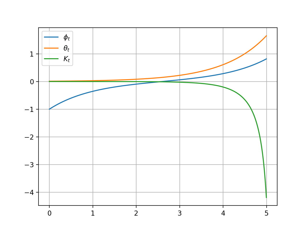
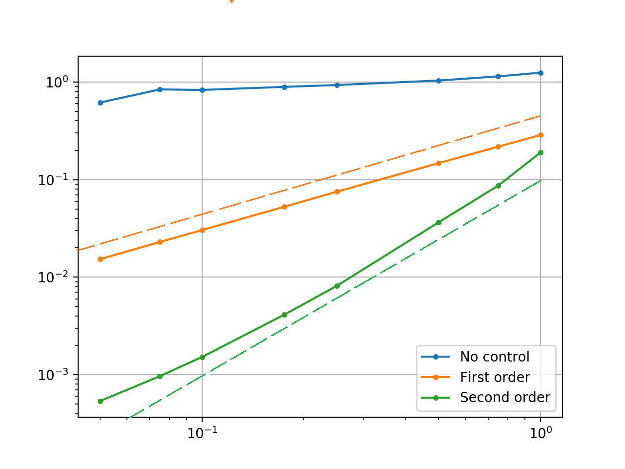
Figure 1: Left: Instanton, momentum and Riccati matrix (here scalar values). Right: Evolution of $R(\varepsilon)$ as defined in (11) with $\varepsilon$ in logarithmic scale, for the unbiased estimator and the dynamics biased by $\hat{g}_{1}^{\varepsilon}$ and $\hat{g}_{2}^{\varepsilon}$. Linear and quadratic decays are plotted in dashed lines.

5 Discussion

This work is concerned with the issue of variance reduction for the Monte Carlo estimation of exponential-like expectations, as they often arise in statistical physics and other areas. Our main goal was to design a framework to assess whether a given approximation of the optimal Hamilton–Jacobi control indeed reduces relative variance as temperature becomes small, and at which scale.

To achieve this, we introduce the notion of stochastic viscosity approximation (SVA), inspired by recent developments on the theory of Feynman–Kac partial differential equations [26]. We believe our definition is meaningful: a SVA approximately solves the Hamilton–Jacobi–Bellman equation along relevant tilted paths. This is precisely what is needed in the Girsanov theorem to make stochastic terms small. We therefore prove an associated variance reduction property. This definition comes in sharp contrast with standard approximation techniques criteria, which typically control a non-local error to assess convergence as a mesh size decays to zero. Here we show that even an approximation that does not depend on temperature or any parameter going to zero can have a vanishing log-efficiency in the zero temperature limit!

Since this study was in part motivated by earlier heuristics on importance sampling [20, 12], we specifically study these approaches. We show, under geometrical conditions, that the first and second order techniques proposed in [20, 12] define stochastic viscosity approximations of order one and two respectively, thus proving variance reduction properties for these heuristics. This also shows that our definition can indeed be applied to actual approximation schemes. A simple numerical example illustrates our results.

As for any new definition, connection between stochastic viscosity solutions and existing works should be explored further. In particular, concerning variance reduction, it seems interesting to understand better the link with the large deviation criteria designed in [21] as well as the more involved Isaacs equations [9]. Moreover, it seems natural to revisit existing approximation techniques and check whether they match our definition and, as already noted in [26], the relation with viscosity solutions of HJB problems should be made clearer, appart from the variance reduction problem.

Finally, although our work gives ground to the schemes based on instanton expansions as the ones presented in Section 4, such schemes do not apply as such when the solution to the instanton problem is not unique, which is the case in many situations. Two ways can be followed to overcome this issue. The first is to extend the approximation to a situation with several instantons, to build a more general abstract expansion of the HJB equation – this is the subject of ongoing investigation of the author. The second, more pragmatic, is to use tools such as the region of strong regularity [16] to update the computation of the instanton at certain times, in the flavour of [22]. Whatever approach is chosen, we believe the notion we introduced in this work is valuable as it quantitatively shows that, when the goal of control is variance reduction, one should focus on approximating the HJB equation along relevant low temperature paths.

References

- [1] L. Angeli, S. Grosskinsky, A. M. Johansen, and A. Pizzoferrato. Rare event simulation for stochastic dynamics in continuous time. J. Stat. Phys., 176(5):1185–1210, 2019.
- [2] G. Barles and E. Jakobsen. Error bounds for monotone approximation schemes for parabolic Hamilton-Jacobi-Bellman equations. Math. Comput., 76(260):1861–1893, 2007.
- [3] G. Barles and E. R. Jakobsen. On the convergence rate of approximation schemes for Hamilton-Jacobi-Bellman equations. ESAIM: Math. Model. Numer. Anal., 36(1):33–54, 2002.
- [4] A. N. Borodin and P. Salminen Handbook of Brownian Motion-Facts and formulae. Springer Science and Business Media. Springer-Verlag, New York, 2015.
- [5] J. Bucklew. Introduction to Rare Event Simulation. Springer Series in Statistics. Springer-Verlag, New York, 2004.
- [6] M. G. Crandall and P.-L. Lions. Two approximations of solutions of Hamilton-Jacobi equations. Math. Comput., 43(167):1–19, 1984.
- [7] P. Del Moral. Feynman-Kac Formulae. Probability and its Applications. Springer, 2004.
- [8] P. Dupuis, A. D. Sezer, and H. Wang. Dynamic importance sampling for queueing networks. Ann. Appl. Probab., 17(4):1306–1346, 2007.
- [9] P. Dupuis and H. Wang. Subsolutions of an Isaacs equation and efficient schemes for importance sampling. Math. Oper. Res., 32(3):723–757, 2007.
- [10] W. E, J. Han, and A. Jentzen. Deep learning-based numerical methods for high-dimensional parabolic partial differential equations and backward stochastic differential equations. Comm. Math. Stat., 5(4):349–380, 2017.
- [11] L. C. Evans. Partial Differential Equations, volume 19 of Graduate Studies in Mathematics. American Mathematical Society, 2010.
- [12] G. Ferré and T. Grafke. Approximate optimal controls via instanton expansion for low temperature free energy computation. SIAM Multiscale Model. Simul., 19(3):1310–1332, 2021.
- [13] G. Ferré and G. Stoltz. Error estimates on ergodic properties of discretized Feynman–Kac semigroups. Numer. Math., 143(2):261–313, 2019.
- [14] G. Ferré and G. Stoltz. Large deviations of empirical measures of diffusions in weighted topologies. Electron. J. Probab., 25:1–52, 2020.
- [15] W. H. Fleming. Exit probabilities and optimal stochastic control. Appl. Math. Optim., 4(1):329–346, 1977.
- [16] W. H. Fleming and M. R. James. Asymptotic series and exit time probabilities. Ann. Probab., pages 1369–1384, 1992.
- [17] W. H. Fleming and H. M. Soner. Controlled Markov Processes and Viscosity Solutions, volume 25 of Stochastic Modelling and Applied Probability. Springer Science & Business Media, 2006.
- [18] M. I. Freidlin and A. D. Wentzell. Random Perturbations of Dynamical Systems, volume 260 of Grundlehren der mathematischen Wissenschaften. Springer, 1998.
- [19] P. Glasserman and Y. Wang. Counterexamples in importance sampling for large deviations probabilities. Ann. Appl. Probab., 7(3):731–746, Aug. 1997.
- [20] T. Grafke and E. Vanden-Eijnden. Numerical computation of rare events via large deviation theory. Chaos: An Interdisciplinary Journal of Nonlinear Science, 29(6):063118, June 2019.
- [21] A. Guyader and H. Touchette. Efficient large deviation estimation based on importance sampling. J. Stat. Phys., 181(2):551–586, 2020.
- [22] M. Hairer and J. Weare. Improved diffusion Monte Carlo. Comm. Pure Appl. Math., 67(12):1995–2021, 2014.
- [23] C. Hartmann and C. Schütte. Efficient rare event simulation by optimal nonequilibrium forcing. J. Stat. Mech. Theory Exp., 2012(11):11004, 2012.
- [24] I. Karatzas and S. Shreve. Brownian Motion and Stochastic Calculus, volume 113 of Graduate Texts in Mathematics. Springer Science & Business Media, 2012.
- [25] T. Lelièvre and G. Stoltz. Partial differential equations and stochastic methods in molecular dynamics. Acta Numer., 25:681–880, 2016.
- [26] C. Léonard. Feynman-Kac formula under a finite entropy condition. Preprint arXiv:2104.09171, 2021.
- [27] A. M. Oberman. Convergent difference schemes for degenerate elliptic and parabolic equations: Hamilton–Jacobi equations and free boundary problems. SIAM J. Numer. Anal., 44(2):879–895, 2006.
- [28] H. Pham. Continuous-Time Stochastic Control and Optimization with Financial Applications, volume 61 of Stochastic Modelling and Applied Probability. Springer Science & Business Media, 2009.
- [29] L. Rey-Bellet. Ergodic properties of Markov processes. In Open Quantum Systems II, pages 1–39. Springer, 2006.
- [30] P. E. Souganidis. Approximation schemes for viscosity solutions of Hamilton-Jacobi equations. J. Differ. Eq., 59(1):1–43, 1985.
- [31] E. Vanden-Eijnden and J. Weare. Rare Event Simulation of Small Noise Diffusions. Comm. Pure Appl. Math., 65(12):1770–1803, Dec. 2012.
- [32] W. Zhang, H. Wang, C. Hartmann, M. Weber, and C. Schütte. Applications of the cross-entropy method to importance sampling and optimal control of diffusions. SIAM J. Sci. Comput., 36(6):A2654–A2672, 2014.