Modulation of pulse profile as a signal for phase transitions in a pulsar core

Abstract

We calculate detailed modification of pulses from a pulsar arising from the effects of phase transition induced density fluctuations on the pulsar moment of inertia. We represent general statistical density fluctuations using a simple model where the initial moment of inertia tensor of the pulsar (taken to be diagonal here) is assumed to get random additional contributions for each of its component which are taken to be Gaussian distributed with certain width characterized by the strength of density fluctuations $\epsilon$. Using sample values of $\epsilon$, (and the pulsar deformation parameter $\eta$) we numerically calculate detailed pulse modifications by solving Euler’s equations for the rotational dynamics of the pulsar. We also give analytical estimates which can be used for arbitrary values of $\epsilon$ and $\eta$. We show that there are very specific patterns in the perturbed pulses which are observable in terms of modulations of pulses over large time periods. In view of the fact that density fluctuations fade away eventually leading to a uniform phase in the interior of pulsar, the off-diagonal components of MI tensor also vanish eventually. Thus, the modification of pulses due to induced wobbling (from the off-diagonal MI components) will also die away eventually. This allows one to distinguish these transient pulse modulations from the effects of any wobbling originally present. Further, the decay of these modulations in time directly relates to relaxation of density fluctuations in the pulsar giving valuable information about the nature of phase transition occurring inside the pulsar.

1 Introduction

For last several decades, QCD phase diagram is being intensely investigated both, on theoretical front as well as on experimental front. The high temperature and low baryon chemical potential regime of strongly interacting matter has been thoroughly studied at RHIC and LHC which have provided compelling evidence for the formation of quark-gluon plasma (QGP). This regime is very interesting as it closely resembles the state of matter during first few microseconds of the early stages of the Universe. There is compelling theoretical evidence that high baryon density regime of QCD provides an extremely rich landscape. Starting with the possibility of transition to high baryon density QGP, there are exotic phases of QCD expected at much larger baryon densities, such as color flavor locked (CFL) phase, 2SC phase, quarkyonic phase, crystalline color superconductor phase etc. (Alford et al., 2008). However, most of these phases are expected to occur at very high values of baryon chemical potential which are difficult to achieve in laboratory experiments. Focused experimental efforts are underway/planned, such as the beam energy scan (BES) program of RHIC, CBM at FAIR, and NICA. Though, the required baryon density for some of these exotic phases may be out of reach in these laboratory experiments.

This regime of very high baryon density in the QCD phase diagram also relates to the cosmos, albeit in a completely different stage of the evolution of the Universe. QCD matter in this regime is expected to occur during present stage of the universe in the cores of compact objects, such as a neutron star, which form at the end of life of normal stars. Baryon densities in the cores of these objects can reach very high values, allowing possibility of these exotic QCD phases to occur.

It then becomes very important to focus efforts on the possibility of observation of these phases in these compact astrophysical objects. Indeed, many signals have been proposed in literature to probe these phases (Heiselberg & Hjorth-Jensen, 1998). Some of us had earlier proposed a technique (Bagchi et al., 2015) to probe the possibility of phase transitions occurring in the interior of a pulsar (which is a rotating neutron star) utilizing the fact that measurements of pulse timings of pulsar signals have reached extraordinary precision, to the level of one part in 10¹⁵. Basic physics of that approach is based on the fact that any phase transition necessarily leads to density fluctuations. These density fluctuations will be statistical in nature, and will be transient, eventually subsiding and leading to the uniform new phase of the matter. Such density fluctuations arising during a phase transition occurring inside the core of a neutron star will lead to transient changes in its moment of inertia (MI) tensor. This will directly affect its rotation, and hence the pulsar timings. With extremely accurate measurements of pulsar timings, very minute changes of moment of inertia of star may be observable, providing a sensitive probe for phase transitions in these objects.

As emphasized in ref. (Bagchi et al., 2015), there are two main aspects of this proposal which can make this technique a powerful probe of phase transitions inside neutron stars. First is that the resulting density fluctuations being statistical in nature, every component of MI tensor will be affected. A typical neutron star has very high degree of symmetry, with extremely tiny difference in different MI values (of order 10${}^{-4}\%$ or less) (Horowitz & Kadau, 2009; Baiko & Chugunov, 2018). Density fluctuations will modify every component of MI tensor, and for a NS rotating about one of its symmetry axes, will generate non-zero off-diagonal components of MI tensor. Consequently, a spinning neutron star will develop wobble (on top of any previously present) which will lead to modulation of the pulse profile as the direction of the beam pointing towards earth will now undergo additional modulation. This is a unique, falsifiable, prediction of this model, and helps in distinguishing such a signal of phase transition from the phenomenon of glitches. This is because standard explanation of glitches invokes de-pinning of vortex clusters in the superfluid core of the NS. Vortices being directed along the rotation axis, primary effect of this de-pinning will be on the spinning rate without significantly perturbing the rotation axis itself. In contrast, density fluctuations from phase transitions will affect diagonal as well as off-diagonal components of MI to same order, thus leading to same order of magnitude effect for the pulse timing as well as the modulation of pulse profile.

The second important feature of this technique relates to the precise nature of density fluctuations. Specific statistical distribution of density fluctuations (Landau & Lifshitz, 1980) arising during a phase transition, and the manner in which these density fluctuations decay away (leading to eventual uniform new phase) crucially depends on the nature of the phase transition. For example, a first order transition proceeding via bubble nucleation leads to specific density fluctuation pattern on the scale of bubble size (Applegate & Hogan, 1985; Kajantie & Hannu, 1986; Applegate et al., 1987; Christiansen & Madsen, 1996; Layek et al., 2001), whereas a transition happening via spinodal decomposition has entirely different distribution of density fluctuations reaching very large length scale. Density fluctuations during a second order phase transition have universal nature (Goldenfeld, 1992), and depend on the specific critical exponents associated with the phase transition.

An entirely different and rich source of information is contained in these density fluctuations for spontaneous symmetry breaking phase transitions if there are associated topological defects. Topological defects can occur in a variety of shapes, from point defects (monopole), to strings, domain walls, and three dimensional structures called as Skyrmions. Formation of topological defects in symmetry breaking transitions is now a very mature field and there is extensive literature on this subject. Dominant mechanism of the formation of topological defects during spontaneous symmetry breaking transitions is via the so called Kibble mechanism (Kibble, 1976, 1980) which was originally proposed for cosmic defects. Subsequently it was realized that this mechanism has completely general applicability (Zurek, 1996). Indeed, it is now used to study topological defect formation during any phase transition, from those occurring in the universe, to a variety of condensed matter systems (Kibble & Srivastava, 2013), and in neutron star cores etc.

These defects can be source of significant density fluctuations depending on the relevant energy scales. Important point is that the defect network resulting from a phase transition and its evolution shows universal characteristics. For example, initial defect density depends only on the relevant correlation length and on the relevant symmetries (and space dimension). Further, the evolution of string defects and domain wall defects shows scaling behavior. These universal properties of defect network and scaling during evolution will be expected to lead to reasonably model independent predictions for changes in the moment of inertia tensor and its time dependence, hence on the effects on pulsar timing, the pulse modification, and specifically, the eventual subsequent relaxation to the original state of rotation. We mention here that there will also be an effect of the new uniform phase on pulsar rotation. Due to free energy difference between the two phases, pulsar rotation frequency will be directly affected. This aspect has been discussed in our earlier work (Bagchi et al., 2015) where the possibility was discussed that such effects may provide an explanation for both glitches and antiglitches in a unified framework. In the present paper, we will not discuss the effects of net changes in the free energy of two phases and will only focus on the effects of density fluctuations. However, we mention here that the effects of free energy difference on pulsar timing and pulse modulations caused by the density fluctuations depend on different sets of parameters. It is possible that the free energy difference may induce changes in pulsar timings which may not be observable at present. In contrast, the pulse modifications due to induced wobbling (from off-diagonal MI terms) may be within reach of observations (we will come back to this point at the end of section 3).

Examples of specific changes in different components of MI tensor, with crude estimates of the magnitudes were given in ref. (Bagchi et al., 2015) for phase transitions between different exotic QCD phases. A particular interesting example of phase transition discussed in ref. (Bagchi et al., 2015) was for the so-called nucleonic superfluid phase. This is not one of the exotic QCD phases alluded to in the discussion above. This is a rather conventional phase expected to occur inside cores of neutron stars, and is of crucial important in explaining the phenomena of glitches. Despite being of much lower energy scale (with the relevant free energy density of order few tenths of MeV) compared to the exotic QCD phases such as the CFL phase (with relevant energy scale being the QCD scale of 200 MeV, or higher depending on the baryon density) even this superfluid phase transition is expected to lead to significant changes in the MI tensor (Bagchi et al., 2015).

We follow up this proposal of Bagchi et al. (2015) in this paper and calculate specific signals resulting from these density fluctuations in terms of its effect on the modification of the pulses of the pulsar. There being too many possibilities for different phase transitions in the pulsar core, we present a general study in this work where the specific details of density fluctuations relating to particular phase transition are ignored. The only relevant part used here is that these are random density fluctuations, and are expected to affect each component of the MI tensor. For simplicity, in this first study of this kind, we make further approximation and assume that the initial moment of inertia tensor $I_{ij}^{0}$ gets additional contribution $\delta I_{ij}$ for each of its component. Initial MI tensor is taken to be diagonal with eigenvalues $I_{33}^{0}=I_{0},$ and $I_{11}^{0}=I_{22}^{0}\equiv I_{T}<I_{0}$. Here $I_{ii}^{0}$ refer to $I_{xx},I_{yy},I_{zz}$ for $i=1,2,3$ respectively. $\delta I_{ij}$ is assumed to be Gaussian distributed with width $\sigma=\epsilon I_{0}$. In view of the estimates in ref. (Bagchi et al., 2015), we consider two specific values of $\epsilon$ $10^{-8}$ to $10^{-5}$ (in order that the pulse modulations are visible in a reasonable time scale for the numerical computations). Though, we give analytical estimates which can be used for even lower values of $\epsilon$ as discussed in ref. (Bagchi et al., 2015) (it is not clear if such low values will lead to pulse modifications which can be currently observed).

We will see that there are very specific patterns in the perturbed pulses which are observable in terms of modulations of pulses over much larger time periods than the basic pulse period. In view of the fact that density fluctuations fade away eventually leading to a uniform phase in the interior of pulsar, the off-diagonal components of MI tensor also vanish eventually. As we will discuss below, as a consequence of this, pulsar restores its original state of rotation completely (apart from any effects resulting from free energy changes between the two phases of the transition as discussed above). In particular the modification of pulses due to induced wobbling (from the off-diagonal MI components) will also die away eventually. This will be crucial in distinguishing these pulse modulations from the effects of any wobbling originally present.

We note that in representing the effect of density fluctuations on MI tensor in terms of Gaussian distributed random components $\delta I_{ij}$ with a single parameter $\epsilon$, we are missing out very useful information about characteristic statistics of the density fluctuations which could differentiate between different types of phase transitions. Thus, the present study is meant to focus on the gross features of the pulse modification, such as the period and amplitude of pulse modification. Next step will be to determine the detailed modification of the MI tensor depending on specific phase transition, and see if observations of the perturbed signal are capable of distinguishing between different phase transitions.

We mention that there have been several theoretical studies on the effects of free precession of pulsars because of its various observational consequences. The studies of pulsar precession have become even more exciting and relevant as there seems to be evidence of free precession, as reported from the observation of the periodic residuals of PSR 1828-11 (Stairs et al., 2000). There was a theoretical proposal (Wasserman, 2003; Akgun et al., 2006) that precession caused by triaxiality of the pulsar can be a possible cause for such behavior of PSR 1828-11. The precession of pulsars is also studied to probe the internal structure of neutrons stars. In this context, modeling the free precession of neutrons stars and by comparing with the observations, the authors Jones & Andersson (2001) have made a few interesting conclusions regarding the crust-core coupling and on the possible role of superfluidity in the free precession of the crust. In our work here, we aim to probe the various phase transitions occurring inside the core of pulsars. Here, the phase transition induced density fluctuation is considered to be responsible for the precession of pulsars affecting the pulse profile.

The paper is organized in the following manner. In section 2, we present the basic formalism for calculating the effects of the modification in the MI tensor by a random matrix resulting from density fluctuations on the state of rotation of the pulsar. Using Euler’s equations, we calculate the rate of change of angular velocities about the principal axes of the pulsar (which, due to density fluctuations, differ from the original principal axes of a symmetric spheroidal shape pulsar). Here we focus on specific points on the surface of the pulsar which are emitting radiation (which, again, for simplicity is taken to be on the surface of the pulsar), and study changes in its trajectory as the pulsar rotation develops wobbling. We then calculate the resulting perturbation in the pulsar signal as observed on the earth. Section 3 discusses parameter choices, initial conditions, and estimates for modulation frequency etc. depending on the magnitudes of $\epsilon$, and $I_{o},I_{T}$. Section 4 presents the algorithm for calculation of the pulse modification and presents numerical results. Section 5 presents discussion of results and various observational aspects. We conclude in section 6 with discussion of various limitations of our procedure, and future possibilities, e.g. possibility of observing details in the perturbed signal which can distinguish between different phase transitions.

2 The effects of density fluctuations on pulsar dynamics : The basic formalism

For the study of pulsar dynamics in the presence of phase transition induced density fluctuations, we take the initial shape of the pulsar to be oblate spheroidal. The pulsar is assumed to be rotating about the symmetry $z$-axis with angular frequency $\omega$ and angular momentum $L_{z}=L$ ($L_{x}=0=L_{y}$). The unperturbed principal moment of inertia (MI) with respect to the body-fixed frame $S$ (Fig. 1) are denoted by $I_{ij}^{0}$ ($i,j=1,2,3$). In brief notations, the diagonal components can be written as, $I_{11}^{0}\equiv I_{1}^{0}$, $I_{22}^{0}\equiv I_{2}^{0}$ with $I^{0}_{1}=I^{0}_{2}$ and $I_{33}^{0}\equiv I_{3}^{0}=I_{0}$ (with $I_{0}>I^{0}_{1},I^{0}_{2}$), and $I_{ij}^{0}=0$ for $i\neq j$. The oblateness of the star is parameterized by $\eta=(I_{0}-I_{1}^{0})/I_{0}$. The value of $\eta$ depends on various properties of the star, such as mass, rigidity of the crust, and the magnetic field etc. There have been several studies where the authors (Horowitz & Kadau, 2009; Baiko & Chugunov, 2018) have carried out detailed molecular dynamical simulations to determine the values of $\eta$ by estimating the crustal breaking strain of neutron stars. Those works have put an upper limit of ellipticity as $\eta\simeq 10^{-6}$. However, the results being sensitive to the modeling of the crust, there are uncertainties in the estimates of breaking strain. In fact, it has been suggested (based on the studies of a magnetar, (Makishima & et. al., 2014)) that the deviation from the sphericity of pulsar can be as high as $\sim 10^{-4}$. From observational perspective, there were several attempts (Abadie & et. al., 2011; Aasi et al., 2014; Abbott et al., 2020) to constrain the deformation parameter of triaxial stars through direct searches for gravitational waves (GWs). For example, a recent result (Abbott et al., 2020) constrained the upper limit of $\eta$ for Crab and Vela pulsars at $10^{-5}$ and $10^{-4}$, respectively. As recorded by Aasi et al. (2014), there are also a few pulsars with extremely high ($\eta\sim 10^{-2}-10^{-3}$) ellipticities.

Note that such constraints are valid for triaxial stars only. It is not possible to put such constraints for the spheroidal pulsars due to the absence of continuous GWs from these sources. However, within these observational limitations and the uncertainties in theoretical estimate, we will take sample values of $\eta$ in the range $10^{-3}-10^{-2}$ for the initial unperturbed pulsars. This is helpful in showing modulations of pulse profile over reasonable time duration. The results can be straightforwardly extended to much smaller values of $\eta$ (which lead to pulse modulations over very long time durations).

As we have mentioned earlier, the phase transitions inside the core of a pulsar inevitably produce density fluctuations (Bagchi et al., 2015), and hence cause perturbation in MI tensor. Importantly, the MI tensor now develops non-zero off-diagonal components causing the star to precess about the z-axis. Detailed simulations were carried out in ref. (Bagchi et al., 2015) to estimate the magnitude of density fluctuations caused by various possible phase transitions inside the core of a pulsar. In those simulations, depending on the types of transitions, the fractional change in the MI tensor $\delta I_{ij}/I_{0}$ were estimated to be of order $\sim 10^{-14}-10^{-6}$ (with the limitation of extrapolating the simulation results of small lattice sizes to realistic NS size). We would like to study the pulsar dynamics in the presence of such perturbations and present results for density fluctuations of this order. As we will see, the results can be straightforwardly extended to arbitrary small values of density fluctuations (though, possibility of observing effects of much smaller density fluctuations on pulse profiles may not be realistic at present stage).

Fig. 1 shows the space fixed frame $S$ (black solid lines) for the unperturbed pulsar (of oblate shape) which is rotating about the z-axis with frequency $\omega$ and angular momentum $L_{z}=L$. Phase transition is assumed to occur at time t = 0 (for simplicity, we assume the transition to be instantaneous) generating density fluctuations. With density fluctuation, the new principal axes of the pulsar at time $t=0$ (after the phase transition) are denoted by ($x_{0}$, $y_{0}$, $z_{0}$). This new body fixed frame $S_{0}$ (at t = 0) is shown by red dotted lines. $S^{\prime}$ frame (with axes $x^{\prime},y^{\prime},z^{\prime}$) denotes this body fixed frame at any arbitrary time $t>0$ and is shown by blue dashed lines.

Let us denote by $I_{1}$, $I_{2}$ and $I_{3}$, the principal MI of the perturbed pulsar with respect to the body fixed frame $S^{\prime}$ (as in Fig. 1). The frame $S^{\prime}$ momentarily coincides (at time $t$) with a space fixed frame, with respect to which the dynamical equations need to be written. The angular frequency of the star about this frame are denoted by $\omega_{1}(t)$, $\omega_{2}(t)$ and $\omega_{3}(t)$, respectively.

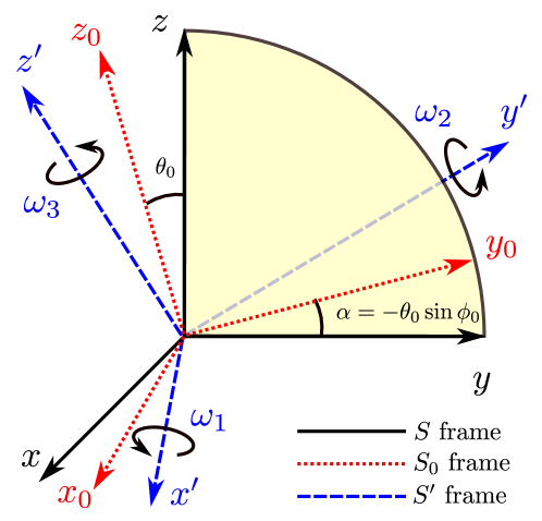
Figure 1: Before phase transition, an oblate shape pulsar is rotating about z-axis with frequency $\omega$ and angular momentum $L_{z}=L$. Black solid lines show the space fixed frame S for the unperturbed pulsar. Orientations of the principal axes ($x_{0}$, $y_{0}$, $z_{0}$) immediately after the phase transition (at $t=0$) of $S_{0}$ frame are shown with red dotted lines. The body-fixed frame $S^{\prime}$ at any arbitrary time $t$ is shown with blue dashed lines.

The set of Euler’s equations which governs the dynamics of the pulsar can now be written as (Goldstein et al., 2013; Kleppner & Kolenkow, 2013)

$$I_{1}\dot{\omega}_{1}-(I_{2}-I_{3})\omega_{2}\omega_{3} =0$$ (1)

$$I_{2}\dot{\omega}_{2}-(I_{3}-I_{1})\omega_{1}\omega_{3} =0$$ (2)

$$I_{3}\dot{\omega}_{3}-(I_{1}-I_{2})\omega_{1}\omega_{2} =0.$$ (3)

We assumed that the angular frequency $\omega$ of the unperturbed state is along the z-axis. As density perturbations are assumed to be small, the value of $\omega_{3}$ is expected to remain close to $\omega$. However, $\omega_{1}$ and $\omega_{2}$ now become non-zero, though much smaller compared to $\omega_{3}$, i.e., $\omega_{1},\omega_{2}<<\omega_{3}$. Thus, within first order in $\omega_{1}$ and $\omega_{2}$, we get from Eq. (3)

$$I_{3}\dot{\omega}_{3}=0\leavevmode\nobreak\ ;\text{i.e.,}\leavevmode\nobreak\ \leavevmode\nobreak\ \omega_{3}=\text{constant}.$$ (4)

Here, we have neglected the higher order term $\omega_{1}\omega_{2}$ in Eq. (3). The dynamics of $\omega_{1}$ can now be obtained by using Eq. (1) and Eq. (2) as

$$\ddot{\omega}_{1}+\Omega^{2}\leavevmode\nobreak\ \omega_{1}=0.$$ (5)

Where, $\Omega=\omega_{3}[(I_{3}-I_{1})(I_{3}-I_{2})/(I_{1}I_{2})]^{1/2}$ is the precession frequency of the pulsars caused by the perturbations. We assume that phase transition induced density fluctuations are sufficiently small so that $I_{3}>I_{1},I_{2}$ condition remains valid even after the phase transition. Thus, $\Omega$ will be real. With this, the solution of Eq. (5) becomes oscillatory,

$$\omega_{1}(t)=A\leavevmode\nobreak\ \cos(\Omega\leavevmode\nobreak\ t)+B\leavevmode\nobreak\ \sin(\Omega\leavevmode\nobreak\ t).$$ (6)

$A$, $B$ are two constants which can be determined from the initial conditions. The solution of $\omega_{2}$ can be obtained by simply finding $\dot{\omega}_{1}$ from Eq. (6), and substituting it in Eq. (1). The resulting solution is given by

$$\omega_{2}(t)=k[A\sin(\Omega\leavevmode\nobreak\ t)-B\cos(\Omega\leavevmode\nobreak\ t)].$$ (7)

Where the overall factor $k$ is given as $k=[I_{1}(I_{3}-I_{1})/(I_{2}(I_{3}-I_{2}))]^{1/2}$. We have set the initial time $t=0$ as the time of completion of the phase transition, which is assumed to be the onset of precession of the pulsar as well. If $\omega_{1}^{0}$ and $\omega_{2}^{0}$ denote the respective angular velocities at $t=0$, the set of solutions (6), (7) can then be rewritten as (using Eqs. (1), (2)),

$$\omega_{1}(t) =\omega_{1}^{0}\cos(\Omega\leavevmode\nobreak\ t)-\frac{\omega_{2}^{0}}{k}\sin(\Omega\leavevmode\nobreak\ t)$$ (8)

$$\omega_{2}(t) =k\omega_{1}^{0}\sin(\Omega\leavevmode\nobreak\ t)+\omega_{2}^{0}\cos(\Omega\leavevmode\nobreak\ t).$$ (9)

Note that the above set of equations still has two arbitrary constants $\omega_{1}^{0}$ and $\omega_{2}^{0}$ to be fixed from the initial conditions. In the next section, we will discuss the procedure of fixing these quantities from the given initial conditions. Along with this, we will also discuss our choice of parameters, and present an estimate of precession frequency $\Omega$. More detailed numerical procedures for obtaining the effects on pulse profiles will be discussed in the subsequent section.

3 Initial conditions, choice of parameters, and estimates for modulation frequency

3.1 Initial conditions

The values of $\omega_{1}^{0}$ and $\omega_{2}^{0}$ in Eqs. (8) and (9) can be determined by using the conservation of angular momentum. Note that there is no external torque on the pulsar, the dynamics is affected solely due to the internal density fluctuations. Thus the angular momentum is conserved. (We are neglecting the possibility of significant emission of any particles during the phase transition.) Prior to the phase transition, the pulsar rotates about the z-axis with angular velocity $\omega$ and the angular momentum has only z-component $L_{z}=L$. After completion of the phase transition at $t=0$, the orientations of the new set of principal axes $x_{0}$, $y_{0}$ and $z_{0}$ of frame $S_{0}$ are changed relative to the original frame $S$ as shown in Fig. 1. The new $y_{0}$-axis is chosen to lie in the y-z plane, making an infinitesimal small angle $\alpha$ (for small perturbations) with the y-axis. Note that for the unperturbed state, the principal axis corresponding to $I_{3}^{0}$ is unambiguously fixed. However, this is not true for the other two axes (since $I_{1}^{0}=I_{2}^{0}$) lying in the x-y plane. We have the freedom of choosing one of them arbitrarily. Here we have exploited this freedom to choose the y-axis (by rotating the x-y plane) in such a way that $y_{0}$-axis lies in the y-z plane. With this choice, we can now write the unit vector along $y_{0}$ as $\hat{y_{0}}=\hat{y}+\alpha\leavevmode\nobreak\ \hat{z}$. Denoting the polar angle and the azimuthal angle of $z_{0}$-axis as $\theta_{0}$ and $\phi_{0}$, respectively (these are the standard angles in spherical coordinates measured relative to S-frame), one can also write the unit vector along $z_{0}$ as $\hat{z_{0}}=\theta_{0}\cos\phi_{0}\leavevmode\nobreak\ \hat{x}+\theta_{0}\sin\phi_{0}\leavevmode\nobreak\ \hat{y}+\hat{z}$. Using orthogonality, the angle $\alpha$ and the unit vector $\hat{x_{0}}$ can be fixed as $\alpha=-\theta_{0}\sin\phi_{0}$ and $\hat{x_{0}}=\hat{x}-\theta_{0}\cos\phi_{0}\leavevmode\nobreak\ \hat{z}$. Note that by expressing the unit vectors ($\hat{x_{0}},\hat{y_{0}},\hat{z_{0}}$) in terms of ($\hat{x},\hat{y},\hat{z}$) allows us to determine the rotational matrix $R_{0}$, which describes the orientations of the new set of principal axes relative to the old set. The matrix $R_{0}$ is parameterized by the angles $(\theta_{0},\phi_{0})$ and can be written as

$$R_{0}=\begin{pmatrix}1&0&-\theta_{0}\cos\phi_{0}\\ 0&1&-\theta_{0}\sin\phi_{0}\\ \theta_{0}\cos\phi_{0}&\theta_{0}\sin\phi_{0}&1\end{pmatrix}$$ (10)

We will see later (section 4) the role of $R_{0}$ in our numerical calculations. The initial angle $\theta_{0}$ and $\phi_{0}$ are determined by diagonalizing the perturbed MI matrix, and finding the eigen vectors corresponding to three eigen values.

With the above choice of orientations of the new set of principal axes, we now resolve the original angular momentum $L_{z}$ ($=L$) along $x_{0}$, $y_{0}$ and $z_{0}$, respectively. The corresponding components can be written as

$$L_{x_{0}}(t=0) =I_{1}\omega_{1}^{0}=-L\theta_{0}\cos\phi_{0}$$ (11)

$$L_{y_{0}}(t=0) =I_{2}\omega_{2}^{0}=-L\theta_{0}\sin\phi_{0}$$ (12)

$$L_{z_{0}}(t=0) =I_{3}\omega_{3}^{0}=L.$$ (13)

Using the above set of equations, the angular frequencies Eq. (4, 8, 9) can be expressed in terms of $\theta_{0}$ and $\phi_{0}$ as

$$\omega_{1}(t) =\dot{\theta}_{1}=-\omega\theta_{0}[\cos\phi_{0}\cos(\Omega t)-\frac{\sin\phi_{0}}{k}\sin(\Omega t)]$$ (14)

$$\omega_{2}(t) =\dot{\theta}_{2}=-\omega\theta_{0}[k\cos\phi_{0}\sin(\Omega t)+\sin\phi_{0}\cos(\Omega t)]$$ (15)

$$\omega_{3}(t) =\dot{\theta}_{3}=\omega.$$ (16)

In the above, we have taken an approximation, $L/I_{1}\simeq L/I_{3}\simeq\omega$. This is in view of Eq. (16) and the fact that angle $\theta_{0}$ is very small for tiny density fluctuations, as we will see below. The numerical algorithm for finding the set of solutions $\theta_{i}(t)$ ($i=1,2,3$), and their role in modulating pulse profiles will also be discussed therein. Now before presenting such numerical prescription, we will provide below a few estimates of various quantities relevant to the precession.

3.2 The choice of parameters and estimates of various quantities characterizing the precession

First, we estimate the precession frequency $\Omega=[(I_{3}-I_{1})(I_{3}-I_{2})/(I_{1}I_{2})]^{1/2}\omega$. As the perturbations $\delta I_{ij}$ are small, the new set of principal axes are expected to be very close to the original (unperturbed) axes. This is also observed numerically to be discussed in the next section. Thus the principal MI of the perturbed state can be written as, $I_{1,2}=I_{0}(1-\eta+\epsilon_{1,2})$ and $I_{3}=I_{0}(1+\epsilon_{3})$. Where, $\epsilon_{i}$ ($i=1,2,3$) are taken to be of order $\epsilon$ for which we will take two sample values, $10^{-8}$ and $10^{-5}$. The precession frequency $\Omega$ can then be expressed in terms of $\eta$ and $\epsilon$ (a function of $\epsilon_{i}\leavevmode\nobreak\$ ; $i=1,2,3$) as

$$\Omega\simeq\frac{\eta+\epsilon}{1-\eta+\epsilon}\omega\simeq\eta\leavevmode\nobreak\ \omega.$$ (17)

Where, as mentioned above we have assumed that $\epsilon,\leavevmode\nobreak\ \eta<<1$ and $\epsilon<<\eta$. Therefore, the precession frequency is completely determined by the deformation parameter $\eta$ of the unperturbed pulsars. Thus, for a millisecond pulsar, for example, the time period of precession will be of order 1 sec, if the deformation parameter is of order $10^{-3}$. We will discuss the implications of this further in section 5.

The amplitude $\omega_{m}$ of frequency oscillations $\omega_{1}(t)$, and the amplitude $\theta_{m}$ of precession angle $\theta_{1}(t)$ can be estimated from Eq. (14). Note that since $k=[I_{1}(I_{3}-I_{1})/(I_{2}(I_{3}-I_{2}))]^{1/2}\simeq 1+\epsilon/2\eta$, the corresponding quantities associated with $\omega_{2}(t)$ will be of same order as for $\omega_{1}(t)$. The relative angular shift $(\theta_{0},\phi_{0})$ of the principal axes (see Fig. 1) are determined by diagonalizing the perturbed matrix $I_{ij}$, and finding the eigen vectors corresponding to three eigen values. These eigen-vectors will then correspond to the set of three principal axes. The identification of $z_{0}$-axis can be done by finding the direction cosines of the eigen-vector corresponding to the largest eigenvalue. Now, as mentioned earlier, the perturbed moment of inertia (MI) matrix elements were taken to be $I_{ij}=I^{0}_{ij}+\delta I_{ij}$. Where $\delta I_{ij}$ is assumed to be Gaussian distributed with width $\sigma=\epsilon I_{0}$ ($I_{0}\equiv I^{0}_{3}$). For an analytical estimate of $\theta_{0}$, let us define a quantity $\epsilon_{ij}$, which characterizes the relative perturbation of MI matrix element due to the density fluctuations as $\epsilon_{ij}=\delta I_{ij}/I_{0}$. As the width $\sigma$ of the perturbations is assumed to be of order $\epsilon I_{0}$, all the components of $\epsilon_{ij}$ ($i,j=1,2,3$) are also expected to be of order $\epsilon$. For a simple analytical estimate, we use the approximation $\epsilon_{ij}=\epsilon/I_{0}$. With this, the diagonalizations of the perturbed matrix gives the result,

$$\cos\theta_{0}=\left(1+2\left(\frac{\epsilon I_{0}}{I_{3}-I_{1}-\epsilon I_{0}}\right)^{2}\right)^{-1/2}.$$ (18)

Substituting $I_{1}=I_{2}\simeq I_{0}(1-\eta+\epsilon)$, $I_{3}\simeq I_{0}(1+\epsilon)$ and assuming $\epsilon<<\eta$, we now get the angular shift of $z^{\prime}$-axis (to leading order in $\epsilon$) as

$$\theta_{0}\simeq\sqrt{2}\leavevmode\nobreak\ \left({\epsilon\over\eta}\right).$$ (19)

Allowing for slightly more general $\epsilon_{ij}$ also gives similar result. The numerical procedure for finding $\theta_{0}$ will be discussed later in section 4. It turns out that for a general random values of $\epsilon_{ij}$, our numerical results also approximately produce the above analytical estimate of $\theta_{0}$.

As $k=[I_{1}(I_{3}-I_{1})/(I_{2}(I_{3}-I_{2}))]^{1/2}\simeq 1+\epsilon/2\eta$, we can now rewrite Eq.(14) and Eq.(15) as

$$\omega_{1}(t) =-\omega\theta_{0}[\cos(\Omega t+\phi_{0})+\frac{\epsilon}{2\eta}\sin\phi_{0}\sin(\Omega t)]$$ (20)

$$\omega_{2}(t) =-\omega\theta_{0}[\sin(\Omega t+\phi_{0})+\frac{\epsilon}{2\eta}\cos\phi_{0}\sin(\Omega t)].$$ (21)

The corresponding rotational angles can be written as

$$\theta_{1}(t) =-\frac{\omega\theta_{0}}{\Omega}[\sin(\Omega t+\phi_{0})-\frac{\epsilon}{2\eta}\sin\phi_{0}\cos(\Omega t)]$$ (22)

$$\theta_{2}(t) =\frac{\omega\theta_{0}}{\Omega}[\cos(\Omega t+\phi_{0})+\frac{\epsilon}{2\eta}\cos\phi_{0}\cos(\Omega t)].$$ (23)

Since $\theta_{0}\simeq\sqrt{2}(\epsilon/\eta)$, the second terms in the above set of equations (Eq. (20) - Eq. (23)) are of order $\sim(\epsilon/\eta)^{2}$. The resulting amplitude $\omega_{m}$ of frequency oscillations $\omega_{1,2}(t)$ (Eq. (20) and Eq. (21)), and the amplitude $\theta_{m}$ of precession angles $\theta_{1,2}$ ((Eq. (22) and Eq. (23)) are thus given by $\omega_{m}=\omega\theta_{0}\simeq\sqrt{2}(\epsilon/\eta)\omega$ and $\theta_{m}=(\omega/\Omega)\theta_{0}\simeq\sqrt{2}\leavevmode\nobreak\ (\epsilon/\eta^{2})$. So for $\eta=10^{-3}$, the oscillation amplitudes for $\theta_{1}$ and $\theta_{2}$ will be of order $10^{6}\leavevmode\nobreak\ \epsilon$. This, for example, results in approximately $1^{\circ}$ amplitude for $\epsilon=10^{-8}$. The observational aspects of this significant result will be discussed in section 5.

The effects of precession will be seen on the observed fluxes from the pulsars. To estimate that, we assume the flux emission to be conical in nature with the vertex of the cone at the centre of the pulsar. The angular flux distribution for the pulsars is taken to be azimuthally symmetric about the centre of the emission region and is taken to be of Gaussian shape (Krishnamohan & Downs, 1983) of width $w$,

$$F(\alpha)=F_{0}\leavevmode\nobreak\ e^{-\frac{\alpha^{2}}{w^{2}}}.$$ (24)

Where $\alpha$ is the angle of the radial vector of the emission point from the central axis of the cone. If the perturbations result in the change of $\alpha$ by a small amount $\delta$, the corresponding change in flux becomes

$$F^{\prime}(\phi)=F_{0}\leavevmode\nobreak\ e^{-\frac{(\alpha+\delta)^{2}}{w^{2}}}\simeq F(\phi)\left(1-2\delta\frac{\alpha}{w^{2}}\right).$$ (25)

Thus we see that the fractional change of flux will be of order $O(\delta)$, which is approximately equal to $\theta_{m}$, i.e., of order $\epsilon/\eta^{2}$. Here, we recall our earlier discussion that the pulse modifications due to induced wobbling (from off-diagonal MI components) may be more easily observable, even if direct effects on the pulsar frequency arising from free energy difference between two thermodynamic phases remain suppressed.

4 The algorithm for studying pulse modulations and the numerical results

We will describe here the numerical approach that was followed to study the effects on pulse profile due to the precession of a pulsar. First, we consider the profile for an unperturbed pulsar rotating freely about the z-axis with frequency $\omega$. We assume the standard conical shape geometry (Gil, 1981; Gil et al., 1984) for the pulse emission region (Fig. 2). The angles of magnetic axis and the line of sight pointing towards earth with the rotation axis are denoted by $\theta_{r}$ and $\theta_{e}$, respectively. Assume P$(R_{r}\sin\theta_{r}\cos\phi_{r},R_{r}\sin\theta_{r}\sin\phi_{r},R_{r}\cos\theta_{r})$ and E$(R_{e}\sin\theta_{e}\cos\phi_{e},R_{e}\sin\theta_{e}\sin\phi_{e},R_{e}\cos\theta_{e})$ to be the center of the pulse emission region, and the intersection point on the emission region by the direction vector towards earth, respectively. Both the points are assumed to be on the surface of the pulsar, and $R_{r}\simeq R_{e}\equiv R$ is the radius (R) of the (almost spherical) pulsar.

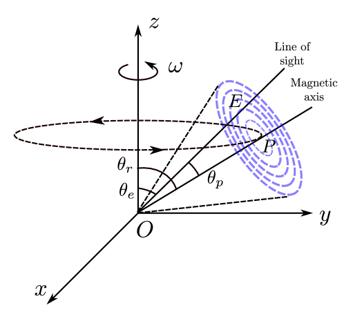
Figure 2: Figure shows the radiation emission cone of a pulsar. The magnetic axis (OP) and the line of sight (OE) pointing towards earth, make angle $\theta_{r}$ and $\theta_{e}$, respectively with the rotation axis. $\theta_{p}$ is the angle between OP and OE.

The angle between $\vec{OE}$ and $\vec{OP}$ is denoted by $\theta_{p}$. Note that $\theta_{p}(t)$ changes with time as the pulse emission cone sweeps across the line of sight with rotation frequency $\dot{\phi}_{r}(t)=\omega$. The evolution of $\theta_{p}$ will be reflected in the observed intensity distribution of the pulses. For that, we take the intensity distribution of pulses as Gaussian (Krishnamohan & Downs, 1983) of width $w$ (as in Eqn.(21)),

$$I(\theta_{p})=I_{0}\leavevmode\nobreak\ e^{-(\theta_{p}^{2}/w^{2})}.$$ (26)

Now, in the presence of density fluctuations, the above profile will be modulated due to the precession of pulsars. For understanding this, let us first set our notations and symbols for various quantities. Let $S(x,y,z)$ be the space-fixed frame (frame of the observer) with respect to which the pulse profile is supposed to be analyzed. $S_{0}(x_{0},y_{0},z_{0})$, $S_{1}(x_{1},y_{1},z_{1})$, …are the instantaneous space-fixed frames, which coincide with the body-fixed frames at time $t=0$ (immediately after the phase transition), $\Delta t,2\Delta t,...$ and so on. At an arbitrary time $t$, the orientations of body-frame axes are determined in terms of the rotations $\theta_{1}(t)$, $\theta_{2}(t)$, and $\theta_{3}(t)$ w.r.t. the corresponding instantaneous space-fixed frame, with corresponding angular frequencies $\omega_{1}(t)$, $\omega_{2}(t)$ and $\omega_{3}(t)$, respectively. Assume an arbitrary fixed point $P^{*}$ on the surface of the (almost perfectly spherical) star, whose angular coordinates with respect to the space-fixed frame $S$ at time $t=0$, are labeled by $(\theta^{*},\phi^{*})$. After the phase transition, at $t=0$, the new principal axes become different, given by the body-fixed frame $S_{0}$, without any rotation occurring for the body. Hence, the location of this point $P^{*}$ w.r.t the body-fixed frame $S_{0}$ will always be given by $R_{0}(\theta^{*},\phi^{*})$ at any time $t$. Here $R_{0}$ is the rotational matrix parameterized by the angles ($\theta_{0},\phi_{0}$) describing the orientations of $S_{0}$-frame relative S-frame (see Eq.(10)). As the body rotates, the corresponding angular coordinates as seen by a space-fixed observer at an arbitrary time $t$ are denoted by $(\theta(t),\phi(t))$. Corresponding Cartesian coordinates will be represented as column vectors while performing coordinate transformation through the operation of rotation matrix. The matrices $R_{x}(\theta_{1})$, $R_{y}(\theta_{2})$ and $R_{z}(\theta_{3})$ describe the rotations by angle $\theta_{1}$ about x-axis, $\theta_{2}$ about y-axis and $\theta_{3}$ about z-axis, respectively. The rotation matrices $R_{0}$, $R_{1}$, …, respectively describe the orientations of ‘$S_{0}$-frame relative to $S$-frame’, ‘$S_{1}$-frame relative to $S_{0}$-frame’,…and so on. These matrices are in turn the products of matrices, $R_{x}$, $R_{y}$ and $R_{z}$. As the rotations are being considered for infinitesimal time period $\Delta t$ w.r.t. the instantaneous space-fixed frames, all the angles are infinitesimal, and $R_{x}$, $R_{y}$ and $R_{z}$ commute with each other.

We will now discuss below our algorithm using which the effect of precession on pulse profile is calculated. As we mentioned above, diagonalization of the perturbed MI matrix gives the new set of principal axes ($S_{0}$-frame in Fig. 1). The orientations of axes of $S_{0}$ relative to those of $S$ is obtained through $R_{0}$ which is parameterized by the initial angles $\theta_{0}$ and $\phi_{0}$ of the $z_{0}$ axis. We noted above that the coordinates of the radiating point $P^{*}$ in the body fixed frame at any time $t$ are fixed, given by $R_{0}(\theta^{*},\phi^{*})$. After this initial set up, following steps are performed to get the pulse profile for the perturbed pulsar.

Step - 1 ($t=\Delta t$) : $\theta_{i}(\Delta t)$, ($i=1,2,3$) is obtained by integrating Eq. (14) - Eq. (16) for a time step $\Delta t$. The matrix $R_{1}$ that describes the orientations of $S_{1}$-frame relative to $S_{0}$-frame is obtained through $R_{1}=R_{x}(\theta_{1})R_{y}(\theta_{2})R_{z}(\theta_{3})$. We then get the location of the point $P^{*}$ at time $t=\Delta t$ as seen by the space-fixed fixed observer (frame $S$) through the coordinate transformations, $[\theta(\Delta t),\phi(\Delta t)]=R_{0}^{-1}R_{1}^{-1}R_{0}(\theta^{*},\phi^{*})$. Note that above prescription is valid for any arbitrary point $P^{*}$ on the surface of the star. For calculating $\theta_{p}$, the point $P^{*}$ is chosen as the center of the emission cone labeled as “P” in Fig. 2. As the star rotates, the angular coordinates of this point change w.r.t. the space fixed frame $S$ leading to changing $\theta_{p}$. Following the same procedure as one would do for the unperturbed pulsars, $\theta_{p}$ is calculated at time $t=\Delta t$ and hence, the intensity of the pulse $I(\theta_{p})$ is obtained from Eq. (26).

Step - 2 ($t=2\Delta t$) : Following the same prescription as above, $\theta_{i}(2\Delta t)$, ($i=1,2,3$) is obtained for the next time step $\Delta t$ (Note, the integration is performed from $\Delta t$ to 2$\Delta t$). This allows to determine the matrix $R_{2}$, which relates $S_{2}$ with $S_{1}$ through $R_{2}=R_{x}(\theta_{1})R_{y}(\theta_{2})R_{z}(\theta_{3})$. The location of $(\theta^{*},\phi^{*})$ at time $2\Delta t$ relative to $S$ is obtained through $[\theta(2\Delta t),\phi(2\Delta t)]=R_{0}^{-1}R_{1}^{-1}R_{2}^{-1}R_{0}(\theta^{*},\phi^{*})$. Again, $I(\theta_{p})$ is obtained at time $t=2\Delta t$ using Eq. (26) .

The above time steps are repeated for a sufficiently long time duration to observe the modulations of the pulse profile due to precession. For clarification, here we should mention that the set of matrices ($R_{1},R_{2},$…) represents the sequence of time evolution. However each of these rotation matrices itself consists of three rotation matrices, about x,y, and z axis, respectively. For example, the matrix $R_{1}$ is given by $R_{1}\equiv(R_{x}({\theta_{1}})R_{y}({\theta_{2}})R_{z}({\theta_{3}}))$, and similarly for $R_{2}$ and so on. We take these three matrices $(R_{x}({\theta_{1}})R_{y}({\theta_{2}})R_{z}({\theta_{3}}))$ to commute as they represent infinitesimal rotations for small time interval $\Delta t$. However, $(R_{1},R_{2},...)$ in sequence represent time integration of rotations. These are naturally time ordered and we do not assume their commutation.

It should also be noted that the calculation of the time evolution of any fixed point due to precession followed by coordinate transformation to S-frame necessitates the appearance of $R_{0}$ matrix twice. The first $R_{0}$ matrix (which now involves two angles $\theta_{0}$ and $\phi_{0}$) gives the coordinates of the radiation point P* in the ($x_{0},y_{0},z_{0}$) frame. The radiation point $P^{*}$ is taken to have coordinates ($\theta^{*},\phi^{*}$) in the original space-fixed frame (which is now given by axes ($x,y,z$). Immediately after the phase transition, the point $P^{*}$ does not move, but the choice of axes now becomes the body fixed frame ($x_{0},y_{0},z_{0}$). The coordinates of $P^{*}$ in this body fixed frame are always given by $R_{0}(P*)$. As the body rotates, at each time step, the location of this point $R_{0}(P*)$ in the body fixed frame has to be transformed to the original space-fixed frame ($x,y,z$). This gives the sequence of matrices $(R_{0}^{-1})(R_{1}^{-1})....$

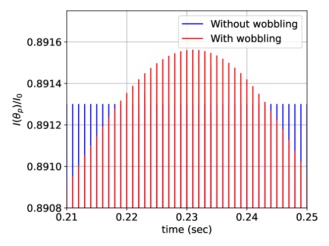
Figure 3: Evolution of normalized pulse intensity $I(\theta_{p})/I_{0}$ with (red color) and without (blue color) modulation (induced by density fluctuations) for a millisecond pulsar, for the parameter set number 1 as listed in Table 1.

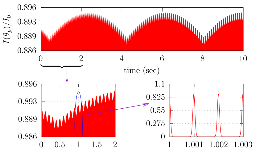
Figure 4: Time evolution of $I(\theta_{p})/I_{0}$ in the presence of density fluctuation induced modulation for the parameter set number 1 in Table 1. Top plot shows the evolution of the top portion of the pulse for a long time duration, clearly showing two different modulation time scales. The plot interior is solid filled up due to crowding of millisecond pulses. Bottom left plot shows the same plot for a smaller time duration for a better resolution, which is further resolved (bottom right) to observe full profiles of a few individual millisecond pulses.

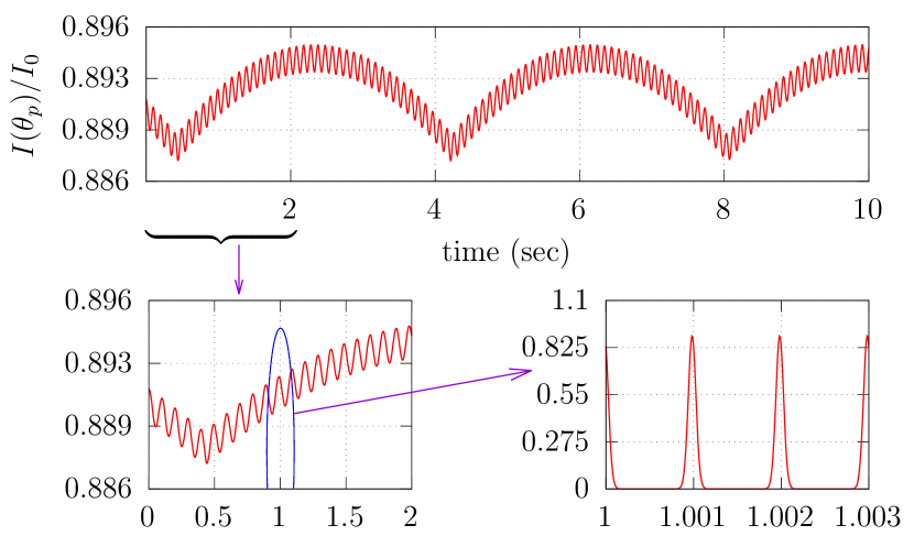
Figure 5: Same plots as in Fig. 4, now only showing the top part of the pulse profiles for clear visibility of the modulated pulse shape details.

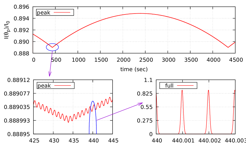
Figure 6: Same plots as in Fig. 5, now for parameter set number 2 in Table 1. Note, flux profile is perfectly smooth in the entire time domain. The apparent kink which appears at time around 435 seconds in the top figure becomes smooth with an improved resolution as shown in the bottom left plot showing expanded plot in that region.

We will now present the results obtained using the above sequence of steps. The parameters used in our calculations are listed in Table 1. A millisecond pulsar is chosen as a candidate for studying the effects of precession on pulse profiles. The angles of magnetic axis and the line of sight pointing towards earth relative to the (unperturbed) rotation axis are taken as $\theta_{r}=45^{\circ}$ and $\theta_{e}=40^{\circ}$, respectively (Fig. 2). The initial (i.e., at $t=0$) azimuthals of the locations P and E (Fig. 2) are taken as $\phi_{r}=45^{\circ}$ and $\phi_{e}=40^{\circ}$, respectively. Note, the choice for $\phi_{r}$ and $\phi_{e}$ at $t=0$ has the same azimuthal separation $\Delta\phi$ as for the angular separation $\Delta\theta$ between $\theta_{r}$ and $\theta_{e}$. The same value of $\Delta\phi$ and $\Delta\theta$ is just an arbitrary choice and in principle, it could be anything. In fact, for other values of $\Delta\phi$, there will simply be a phase shift in the modulation. Now, as mentioned earlier, the change in MI components $\delta I_{ij}$ caused by the density fluctuations are assumed to be Gaussian (Krishnamohan & Downs, 1983) with width $\sigma=\epsilon I_{0}$. The estimates in ref. (Bagchi et al., 2015), suggested that the values of $\epsilon$ may lie in the range $10^{-14}$ to $10^{-6}$. Here, for a case study, we choose two sample values of $\epsilon$ as $10^{-8}$ and $10^{-5}$. We also use two values of the deformation parameter $\eta$ of the assumed oblate shape pulsar as $\eta=10^{-3}$ and $\eta=10^{-2}$. (We again emphasize, we use these parameter values so that different modulations have reasonable time period which can be seen in our numerical simulations. The results are easily extended to much smaller values of $\epsilon$ as well as $\eta$, which usually will lead to very long time scales of modulations.) Note that the parameters $\eta$ and $\epsilon$ set the time scales for the expected flux modulations of the pulses due to the precession. As we discussed above, this can be understood from the equations of motion (Eq. 14 and Eq. 15) for $\omega_{1}$ (or $\omega_{2}$), which is given as $w_{1}\sim\omega_{m}\cos(\Omega t)$. Thus, the time period $T_{\Omega}$ corresponding to the precession frequency $\Omega$ should set one of the time scales for the flux modulation. Now, we see from Eq. (17) that (with our choice $\epsilon<<\eta$), the precession frequency depends only on the pre-existing deformation parameter $\eta$ through $\Omega\simeq\eta\omega$. Thus, for a pulsar with time period $T_{\omega}=10^{-3}$ s, the characteristic time scale $T_{\Omega}=T_{\omega}/\eta$ turns out to be about 0.1 second for $\eta=10^{-2}$ and one second for $\eta=10^{-3}$. As we will see below, this is precisely what we see with our numerical results.

Other than this modulation (let us call it as the first modulation), there will be another modulation time scale. This is because $\omega_{1}$ and $\omega_{2}$ also describe periodic motions about $x$ and $y$ axis respectively. This should lead to another (say, the second modulation) of the millisecond pulses. The amplitude of $\omega_{1}$ oscillation is $\omega_{m}$ (Eq. (20)), similar for $\omega_{2}$, as $k\simeq 1$. With $\omega_{m}\sim(\epsilon/\eta)\omega=(2\pi\epsilon/\eta)1000$ /sec., we expect the second modulation time scale to be determined by the time scale $T_{m}\simeq 10^{-3}\leavevmode\nobreak\ (\eta/\epsilon)$ sec. The value of $T_{m}$ is of order of few seconds for $(\eta,\epsilon)=(10^{-2},10^{-5}$), and a few hundred seconds for $(\eta,\epsilon)=(10^{-3},10^{-8})$. Note that this is the smallest value of second modulation time scale expected because $\omega_{m}$ gives largest value of $\omega_{1}$ (and $\omega_{2}$), being the amplitude of $\omega_{1},\omega_{2}$ oscillations. As $\omega_{1}(\omega_{2})$ oscillates with frequency $\Omega$, changing in magnitude from 0 to $\omega_{m}$, the final time scale for the second modulation will be larger than the value $T_{m}$ estimated above. Further, the complexity of precession of a rigid body in the presence of three rotations about the three axes can only be handled through the numerical simulations. Our numerical results show that, indeed, there is a second modulation time scale of the pulses, and that its time scale is larger by almost on order of magnitude than the value of $T_{m}$ estimated above.

For the initial Gaussian intensity distribution (Eq. (26)) we take the angular width $w=15^{\circ}$. The results from our numerical analysis are shown in Fig. 3 to Fig. 6. For the time evolution of pulses, and calculations of $\theta_{p}(t)$ and $I(\theta_{p})$, simulations are performed with time step $dt=10^{-5}$ sec. This corresponds to total hundred time steps for each oscillation of a millisecond pulse. The time evolution of the normalized flux $I(\theta_{p})/I_{0}$ is shown in Fig. 3 for parameter set no.1 (see Table 1 for the choice of parameters). The red and blue colors, respectively, represent the evolution of the above quantities with and without precession. The effects of precession of pulsar are clearly imprinted in the modulation of $I(\theta_{p})/I_{0}$. The time scale $T_{\Omega}$ of about 0.1 second for this parameter set for the first flux modulation is also visible in Fig. 3. Due to small time duration of the plot, the second modulation is not visible in this plot.

Fig. 4 shows the long time evolution of the pulse profile ($I(\theta_{p})/I_{0}$) in the presence of density fluctuation induced precession for parameter set no.1 in Table 1. This also shows the second modulation, with typical time scale of roughly 5 seconds. Recall, we estimated a time scale of about 1 sec. for this second modulation (for this parameter set). However, as discussed above, this is because of using maximum value $\omega_{m}$ for $\omega_{1}$ and $\omega_{2}$, and it is perfectly reasonable to get a larger time scale for this second modulation. Top plot shows the evolution of the top portion of the pulse, clearly showing the two different modulation time scales. The plot interior is solid filled up due to crowding of millisecond pulses. Bottom left plot shows the same plot for a smaller time duration for a better resolution, which is further resolved (bottom right) to observe full profiles of a few individual millisecond pulses. Fig. 5 shows the same plot as in Fig. 4, but only showing the top of the pulse profiles for clear visibility of the modulated pulse shape details.

Simulations were also performed for a longer time duration for the parameters set number 2 in Table 1. The results are shown in Fig. 6. Here we only show the top of the pulse profile for clear visibility (as in Fig. 5 for parameter set no.1). The top figure shows the long time period modulation (the second modulation) with time scale of few thousand seconds. We had estimated time scale for the second modulation for this case to be few hundred seconds. As discussed above for Fig. 5, longer time period for second modulation is reasonable to expect. Note, flux profile is perfectly smooth in the entire time domain. The apparent kink which appears at time around 435 seconds becomes smooth with an improved resolution as shown in the bottom left plot showing expanded plot in that region. The characteristic time scale for the first flux modulation is clearly observed in this zoomed plot and is of order one second, which agrees with our analytical estimate of $T_{\Omega}$ for this parameter set.

Table 1: Values of various parameters used in our calculations are listed below. The parameter $\eta$ characterizes the deformation of the pulsar, and $\epsilon$ is the fractional change of MI arising due to density fluctuations. The angular width of the assumed Gaussian shape pulse profile is denoted by $w$. $\theta_{r}$ and $\theta_{e}$ are the polar angles of the magnetic axis, and the line of sight pointing towards earth w.r.t. the rotation axis, respectively.

Set number	$\eta$	$\epsilon$	$w$	$\theta_{r}$	$\theta_{e}$
1	$10^{-2}$	$10^{-5}$	$15^{\circ}$	$45^{\circ}$	$40^{\circ}$
2	$10^{-3}$	$10^{-8}$	$15^{\circ}$	$45^{\circ}$	$40^{\circ}$

5 Various observational aspects of our results

It is important to realize that the pulse modulations discussed here resulting from wobbling of pulsar due to density fluctuation will be necessarily transient. As the density fluctuations dissipate away, the pulsar will restore its original state of rotation (apart from any effects of free energy changes to the new uniform phase as discussed above). This should help in disentangling the phase transition induced modulation from any other modulations present for the pulsar (e.g. due to any permanent non-uniformities in the pulsar). One should look for transient changes in pulse profile for any signal of phase transitions. We should mention that by no means we imply that these two modulations are the only possible features of the effects of phase transition induced density fluctuations on the pulses. We have identified these two modulations as clear and distinct features. It will be interesting to find any other possible hidden patterns in these modified pulses. For example, Jones & Andersson (2001) (see also (Wasserman, 2003; Akgun et al., 2006)) have studied the effects of precession on various aspects of electromagnetic signal, such as arrival time residuals, pulse polarisation etc., arising from the electromagnetic spin-down torque. It will be interesting to quantify such effects in our model, where the pulsar precession is induced by density perturbations.

In our present study, the time scale of the first modulation, with a shorter time scale should be possible to see in the pulsar data easily. The observation of longer time modulation may be much more difficult. It will depend on the entire time scale of the completion of the phase transition. If the transition is completed (to a uniform new phase with no density fluctuations present any more) in a relatively short period (compared to the expected time scale of the second modulation), then only small part of the modulation may be visible, and not the whole cycle. This also brings in another important feature of these modulations. As we have seen, the modulation time periods, as well as the amplitude of modulation are proportional to the magnitude of density fluctuations (characterized by $\epsilon$ here). The manner in which the density fluctuations decay away after a phase transition depends crucially on the nature of the transition. For example, during a first order phase transition, density fluctuations typically decay away with the time scale of coalescence of bubbles. For a continuous transition, density fluctuations show scaling pattern with universal scaling exponents. Very interesting possibilities arise when there are topological defects produced in a phase transition. Coarsening of domain wall defects, string defects etc. have been very well studied in literature (see for example the review (Brandenberger, 1994)) and it is known that density fluctuations due to these have specific scaling exponents, with energy density scaling with time as $t^{-b}$ . Analytical calculations, as well as numerical simulations show that $b=1$ for string defects (see (Toyoki & Honda, 1987) and (Nishimori & Nukii, 1989)). Thus, by making detailed observation of the changes in the pulse modulation amplitude as well as modulation period, one should be able to identify the source of density fluctuation, and hence the specific symmetry breaking pattern associated with the phase transition occurring inside the pulsar. We again remind the reader that high density QCD transitions can lead to variety of topological defects. For example, transition to CFL phase, as well as the nucleonic superfluid transition can lead to string defects.

One important implication of our analysis points to a sort of memory effect in the pulsar signal. As we mentioned, after all density fluctuations fade away and uniform phase is achieved, the original state of rotation will be restored, without any wobbling effects. So no modulation of pulse profile will survive (assuming negligible effects on pulsar frequency due to free energy difference between the two phases). However, original state of rotation only means original angular velocities about the original, unperturbed, principal axes. It does not mean that one will get exactly same angular coordinates (say, of the radiation emitting region) in later stages, as one would have obtained in the absence of any phase transition. With intermediate change in the state of rotation (angular velocities as well as new rotated principal axes), the location of the angular coordinates at the complete end of phase transition will depend on various details of the intermediate stage, along with the duration and rate of restoration of the original state of rotation. In fact, in general one will expect a shift in the angular position of the emitting region. Thus, there should be a residual time shift in the pulsar signal for any time after the end of the phase transition. Presence of any such residual time shift in the pulsar signal can thus be attributed to an earlier phase transition stage which could have been missed in direct detection (say, by the modulation of pulses as discussed in this paper). Of course, as discussed in (Jones & Andersson, 2001) a residual time shift can have different origins as well.

6 Conclusion

We have calculated detailed modification of pulses from a pulsar arising from the effects of phase transition induced density fluctuations on the pulsar moment of inertia. To represent a general situation of such statistical density fluctuations, we have used a simple model where the initial moment of inertia tensor $I_{ij}^{0}$ of the pulsar is assumed to get a random additional contribution $\delta I_{ij}$ for each of its component where $\delta I_{ij}$ is taken to be Gaussian distributed with width $\sigma=\epsilon I_{0}$. Using sample values of $\epsilon$ and the pulsar deformation parameter $\eta$, we numerically calculate detailed pulse modifications by solving Euler’s equations for the rotational dynamics of the pulsar. We also give analytical estimates which can be used for arbitrary values of $\epsilon$, though for very small values, the resulting pulse modifications may be beyond current observations. We show that there are very specific patterns in the perturbed pulses which are observable in terms of modulations of pulses over large time periods. In view of the fact that density fluctuations fade away eventually leading to a uniform phase in the interior of pulsar, the off-diagonal components of MI tensor also vanish eventually. Thus, the modification of pulses due to induced wobbling (from the off-diagonal MI components) will also die away eventually. This allows one to distinguish these pulse modulations from the effects of any wobbling originally present. Though, even at such late stages when all density fluctuations die away and no pulse modulation survives, one will expect, in general, a residual time shift of the pulses as restoration of original angular velocities does not imply restoration of the angular orientations as per the original pulses. Such a residual time shift in a pulsar signal could thus be attributed to an earlier phase transition.

We emphasize that in representing the effect of density fluctuations on MI tensor in terms of Gaussian distributed components $\delta I_{ij}$ with a single parameter $\epsilon$, we have ignored details of characteristic statistics of the density fluctuations which could differentiate between different types of phase transitions. Thus, the present study is meant to focus on the gross features of the pulse modification, such as the period and amplitude of pulse modification. We plan to consider detailed modification of the MI tensor depending on specific phase transition, and see if observations of the perturbed signal are capable of distinguishing between different phase transitions. In the present analysis also, some information of the details of phase transition is contained in the manner in which density fluctuations decay away. In particular for a continuous transition, or for topological defect induced density fluctuations, density fluctuations decay away with specific universal exponents, which may be observable by making details analysis of pulse modulations.

7 Acknowledgments

P. Bagchi would like to thank P. Zhuang (Physics department, Tsinghua University) and the Tsinghua University for the financial support during this work. We thank the anonymous reviewer for pointing out an error and constructive suggestions on our earlier manuscript.

8 Data Availability

No new data were generated or analysed in support of this research.

References

- Aasi et al. (2014) Aasi J., Abadie J., et. al. 2014, ApJ, 785, 119
- Abadie & et. al. (2011) Abadie J., et. al. 2011, Phys. Rev. D, 83, 042001
- Abbott et al. (2020) Abbott R., Abbott T. D., Abraham S., et. al. 2020, Astrophys. J. Lett., 902:L21, 17pp
- Akgun et al. (2006) Akgun T., Link B., Wasserman I., 2006, MNRAS, 365, 653
- Alford et al. (2008) Alford M. G., Schmitt A., Rajagopal K., Schafer T., 2008, Rev. Mod. Phys., 80, 1455
- Applegate & Hogan (1985) Applegate J. H., Hogan C. J., 1985, Phys. Rev. D, 31, 3037
- Applegate et al. (1987) Applegate J. H., Hogan C. J., Scherrer R. J., 1987, Phys. Rev. D, 35, 1151
- Bagchi et al. (2015) Bagchi P., Das A., Layek B., Srivastava A. M., 2015, Phys. Lett. B, 747, 120
- Baiko & Chugunov (2018) Baiko D. A., Chugunov A. I., 2018, MNRAS, 480, 5511
- Brandenberger (1994) Brandenberger R. H., 1994, Int. J. Mod. Phys. A, 9, 2117
- Christiansen & Madsen (1996) Christiansen M. B., Madsen J., 1996, Phys. Rev. D, 53, 5446
- Gil (1981) Gil J., 1981, Astron. Astrophys., 104, 69
- Gil et al. (1984) Gil J., Gronkowski P., Rudnicki W., 1984, Astron. Astrophys., 132, 312
- Goldenfeld (1992) Goldenfeld N., 1992, Lectures on Phase Transitions and the Renormalization Group, Westview Press
- Goldstein et al. (2013) Goldstein H., Poole C., Safko J., 2013, Classical Mechanics, 3rd ed., Pearson
- Heiselberg & Hjorth-Jensen (1998) Heiselberg H., Hjorth-Jensen M., 1998, Phys. Rev. Lett., 80, 5485
- Horowitz & Kadau (2009) Horowitz C. J., Kadau K., 2009, Phys. Rev. Lett., 102, 191102
- Jones & Andersson (2001) Jones D. I., Andersson N., 2001, MNRAS, 324, 811
- Kajantie & Hannu (1986) Kajantie K., Hannu K. S., 1986, Phys. Rev. D, 34, 1719
- Kibble (1976) Kibble T. W. B., 1976, J. Phys. A : Math. Gen., 9, 1387
- Kibble (1980) Kibble T. W. B., 1980, Phys. Rep., 67, 183
- Kibble & Srivastava (2013) Kibble T. W. B., Srivastava A. M., 2013, Guest editors, J. Phys. : Condens. Matter, special section on “condensed matter analogues of cosmology”, 25, 400301
- Kleppner & Kolenkow (2013) Kleppner K., Kolenkow R., 2013, An Introduction to Mechanics, 2nd ed., Cambridge University Press
- Krishnamohan & Downs (1983) Krishnamohan S., Downs G. S., 1983, ApJ, 265, 372
- Landau & Lifshitz (1980) Landau L. D., Lifshitz E. M., 1980, Statistical Physics, 3rd ed., Pergamon Press, Vol. 5
- Layek et al. (2001) Layek B., Sanyal S., Srivastava A. M., 2001, Phys. Rev. D, 63, 083512
- Makishima & et. al. (2014) Makishima K., et. al. 2014, Phys. Rev. Lett., 112, 171102
- Nishimori & Nukii (1989) Nishimori H., Nukii T., 1989, J. Phys. Soc. Jpn., 58, 563
- Stairs et al. (2000) Stairs I. H., Lyne A. G., Shemar S. L., 2000, NATURE, 406, 484
- Toyoki & Honda (1987) Toyoki H., Honda K., 1987, Prog. Theor. Phys., 78, 237
- Wasserman (2003) Wasserman I., 2003, MNRAS, 324, 1020
- Zurek (1996) Zurek W. H., 1996, Phys. Rept., 276, 177