Fidelity-mediated analysis of the transverse-field $XY$ chain with the long-range interactions: Anisotropy-driven multi-criticality

Abstract

The transverse-field $XY$ chain with the long-range interactions was investigated by means of the exact-diagonalization method. The algebraic decay rate $\sigma$ of the long-range interaction is related to the effective dimensionality $D(\sigma)$, which governs the criticality of the transverse-field-driven phase transition at $H=H_{c}$. According to the large-$N$ analysis, the phase boundary $H_{c}(\eta)$ exhibits a reentrant behavior within $2<D<3.065\dots$, as the $XY$-anisotropy $\eta$ changes. On the one hand, as for the $D=(2+1)$ and $(1+1)$ short-range $XY$ magnets, the singularities have been determined as $H_{c}(\eta)-H_{c}(0)\sim|\eta|$ and $0$, respectively, and the transient behavior around $D\approx 2.5$ remains unclear. As a preliminary survey, setting $(\sigma,\eta)=(1,0.5)$, we investigate the phase transition by the agency of the fidelity, which seems to detect the singularity at $H=H_{c}$ rather sensitively. Thereby, under the setting $\sigma=4/3$ ($D=2.5$), we cast the fidelity data into the crossover-scaling formula with the properly scaled $\eta$, aiming to determine the multi-criticality around $\eta=0$. Our result indicates that the multi-criticality is identical to that of the $D=(2+1)$ magnet, and $H_{c}(\eta)$’s linearity might be retained down to $D>2$.

1 Introduction

The $XY$ chain with the transverse field is attracting much attention Maziero10 ; Sun14 ; Karpat14 in the context of the quantum information theory Luo18 ; Steane98 ; Bennett00 . A key ingredient is that the model covers both the $XX$- and $XY$-symmetric cases, and a variety of phase transitions occur, as the transverse field and the $XY$-anisotropy change. Meanwhile, its extention to the long-range-interaction case has been made Adelhardt20 ; particularly, the limiting cases such as the transverse-field Ising and $XXZ$ chains with the long-range interactions have been investigated in depth Defenu17 ; Dutta01 ; Koffel12 ; Campana10 ; Gong16 ; Fey16 ; Maghrebi17 ; Frerot17 ; Roy18 ; Puebla19 . A notable point is that the effective dimensionality Defenu17

$$D=2/\sigma+1,$$ (1)

varies, as the decay rate $\sigma$ of the long-range interactions obeying the power law, $1/r^{1+\sigma}$ ($r$: distance between spins), changes. The effective dimensionality $D$ governs the criticality of the transverse-field-driven phase transition. In fact, the $D$ dependence on the criticality for the classical counterpart Fisher72 ; Sak73 ; Gori17 ; Angelini14 ; Joyce66 has been studied extensively. A peculiarity of the quantum magnet is that the long-range interaction induces the asymmetry between the real-space and imaginary-time directions characterized by the dynamical critical exponent $z\neq 1$ Defenu17 . Hence, it is significant to access to the ground state (infinite imaginary-time system size) directly so as to get rid of the influences caused by the aspect ratio between the real-space and imaginary-time system sizes.

In this paper, we investigate the transverse-field $XY$ chain with the long-range interactions Adelhardt20 by means of the exact-diagonalization method, which enables us to access to the ground state directly. We devote ourselves to the anisotropy-driven multi-criticality around the $XX$-symmetric point. So far, the transverse-field-driven criticality with the fixed anisotropy has been explored in detail Adelhardt20 . As for the large-$N$ magnet, the multi-criticality has been studied Wald15 , and an intriguing reentrant behavior was observed in low dimensions, $2<D<3.065\dots$. On the contrary, as for the $XY$ magnet. only the cases of $D=(2+1)$ Wald15 ; Henkel84 ; Jalal16 ; Nishiyama19 and $(1+1)$ Mukherjee11 have been studied, and the transient behavior in between, $D\approx 2.5$, remains unclear. The aim of this paper is to shed light on such a fractional-effective-dimensionality regime by adjusting the algebraic decay rate $\sigma$ of the long-range interactions carefully with the aid of the $\sigma\leftrightarrow D$ relation, Eq. (1).

To be specific, we present the Hamiltonian for the transverse-field $XY$ chain with the long-range interactions

$${\cal H}=-\frac{1}{{\cal N}}\sum_{i\neq j}J_{ij}((1+\eta)S_{i}^{x}S_{j}^{x}+(1-\eta)S^{y}_{i}S^{y}_{j})-H\sum_{i=1}^{N}S^{z}_{i}.$$ (2)

Here, the quantum spin-$1/2$ operator ${\mathbf{S}}_{i}$ is placed at each lattice point, $i=1,2,\dots,N$. The parameters, $H$ and $\eta$, denote the transverse field and $XY$ anisotropy, respectively. The $XY$ interaction between the $i$-$j$ spins decays algebraically as

$$J_{ij}=1/\sin(\pi|i-j|/N)^{1+\sigma},$$ (3)

with the decay rate $\sigma$, and the periodic boundary condition is imposed, i.e. ${\mathbf{S}}_{N+1}={\mathbf{S}}_{1}$, among the alignment of spins, $\{{\mathbf{S}}_{i}\}$. The denominator ${\cal N}$ stands for the Kac factor Homrighausen17 ; Vanderstraeten18

$${\cal N}=\frac{2}{N}\sum_{i\neq j}1/\sin(\pi|i-j|/N)^{1+\sigma}.$$ (4)

As shown in Eq. (1), the effective dimensionality $D=2/\sigma+1$ depends on the decay rate $\sigma$, which thus governs the criticality of the transverse-field-driven phase transition. Even quantitatively, the critical exponent for the $D=3$ Ising model was pursued Goll18 by the $\sigma\leftrightarrow D$ correspondence. In Fig. 1, we present the criticality chart for the $XY$ case ($\eta\neq 1$) Defenu17 ; Dutta01 . For small $\sigma\leq 2/3$, the effective dimensionality $D=4$ is realized, and the transverse-field-driven criticality belongs to the mean-field type. On the contrary, for $\sigma\gtrsim 1.75$, the renormalization-group analysis Defenu17 indicates that the long-range interaction becomes irrelevant, and the criticality reduces to that of the short-range magnet; namely, the $D=2[=(1+1)]$ universality class is realized in this regime. The threshold $\sigma\approx 1.75$ depends on the internal symmetry group, namely, either the $XX$- ($\eta=0$) or $XY$-symmetric ($\eta\neq 0$) type Defenu17 . For the intermediate regime $2/3<\sigma\lesssim 1.75$, the effective dimensionality ranges within $2<D<4$. Rather technically, around both upper and lower thresholds, there emerge notorious logarithmic corrections Fey16 ; Luijten02 ; Brezin14 ; Defenu15 , and these regimes lie off the present concern nonetheless.

Figure 1: The criticality chart Defenu17 ; Dutta01 for the transverse-field $XY$ chain with the long-range interactions (2) is presented. The $XY$ case $\eta\neq 0$ is assumed. As the algebraic decay rate $\sigma$ varies, there appear a number of universality classes as to the transverse-field-driven phase transition successively. For the small decay rate $\sigma\leq 2/3$, the criticality belongs to the mean-field type with the effective dimensionality $D=4$. On the contrary, for $\sigma\gtrsim 1.75$, the ordinary short-range $D=2[=(1+1)]$ universality comes out. In the intermediate regime $2/3<\sigma\lesssim 1.75$, the criticality changes continuously, characterized by the effective dimensionality ranging within $2<D<4$. The upper and lower thresholds, $\sigma\approx 1.75$ and $2/3$, are affected by notorious logarithmic corrections Fey16 ; Luijten02 ; Brezin14 ; Defenu15 , and these regimes lie off the present concern nonetheless.

So far, the transverse-field-driven phase transition at $H=H_{c}(\eta)$ with the fixed anisotropy $\eta$ has been investigated extensively by means of the exact-diagonalization Fey16 ; Homrighausen17 , series-expansion Adelhardt20 ; Fey16 , matrix-product-state Koffel12 ; Vanderstraeten18 and density-matrix-renormalization-group Frerot17 ; Zhu18 methods. On the contrary, little attention has been paid to the anisotropy-driven criticality, namely, the multi-criticality at the $XX$-symmetric point $\eta=0$. As shown in Fig. 2, for the large-$N$ magnet Wald15 , the phase boundary $H_{c}(\eta)$ exhibits a reentrant behavior in low dimensions, $(1+1)<D<(2.065+1)$. Such a feature indicates a counterintuitive picture that lower symmetry group indices the disorder phase in the vicinity of the multi-critical point. On the one hand, as for the short-range $XY$ magnet, only the cases of $D=(2+1)$ Wald15 ; Henkel84 ; Jalal16 ; Nishiyama19 and $(1+1)$ Mukherjee11 have been considered. The former shows the multi-criticality Riedel69 ; Pfeuty74 $H_{c}(\eta)-H_{c}(0)\sim|\eta|^{1/\phi}$ with the crossover exponent $\phi=1$, whereas the latter exhibits no singularity $H_{c}(\eta)-H_{c}(0)=0$ at all. Then, there arises a problem how the crossover exponent behaves at a transient point $D=2.5$. It might be anticipated that $H_{c}(\eta)$’s slope grows monotonically with $\phi=1$ retained, as the dimensionality $D$ increases. However, in principle, the phase boundary can be curved convexly, accompanied with a suppressed exponent $\phi<1$ in such a low-dimensionality regime. The aim of this paper is to explore the multi-criticality for the transient dimensionality by adjusting the decay rate $\sigma$ for the long-range $XY$ magnet (2).

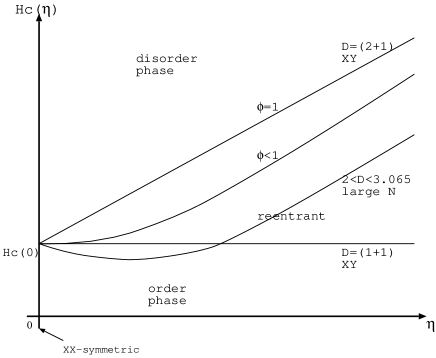
Figure 2: A schematic drawing of the transverse-field-driven phase boundary $H_{c}(\eta)$ with the $XY$ anisotropy $\eta$ for the transverse-field $XY$ model, is presented. The short-range $D=(2+1)$-dimensional $XY$ magnet Wald15 ; Henkel84 ; Jalal16 ; Nishiyama19 exhibits a linear increase of $H_{c}(\eta)-H_{c}(0)\sim|\eta|^{1/\phi}$ with the crossover exponent $\phi=1$ Riedel69 ; Pfeuty74 , whereas the $D=(1+1)$ model Mukherjee11 shows no singularity, i.e., $H_{c}(\eta)={\rm const.}$, at all. It is not clear whether the crossover exponent $\phi$ changes for the intermediate dimensionality such as $D=2.5$; in principle, it can be curved convexly, $\phi<1$. Actually, as for the large-$N$ magnet Wald15 , there appear a reentrant behavior in low dimensions $(1+1)<D<(2.065+1)$.

As a probe to detect the phase transition Quan06 ; Zanardi06 ; HQZhou08 ; Yu09 ; You11 , we resort to the fidelity Uhlmann76 ; Jozsa94 ; Peres84 ; Gorin06

$$F(H,\Delta H)=|\langle H|H+\Delta H\rangle|,$$ (5)

with the ground states, $|H\rangle$ and $|H+\Delta H\rangle$, for the proximate interaction parameters, $H$ and $H+\Delta H$, respectively. The fidelity (5) is readily accessible via the exact-diagonalization method, which admits the ground-state vector $|H\rangle$ explicitly. Moreover, the fidelity does not rely on any presumptions as to the order parameters involved Wang15 , and it is sensitive to generic types of phase transitions such as the $XX$- ($\eta=0$) and $XY$-symmetric ($\eta\neq 0$) cases. In fairness, it has to be mentioned that the information-theoretical quantifier, the so-called genuine multipartite entanglement, detects the phase boundary $H_{c}(\eta)$ clearly for rather restricted system sizes, $N\leq 20$ Roy18 . In this paper, we treated the cluster with $N\leq 32$ spins, taking the advantage in that the fidelity (5) is computationally less demanding,

The rest of this paper is organized as follows. In Sec. 2, the numerical results are presented. In the last section, we address the summary and discussions.

2 Numerical results

In this section, we present the numerical results for the transverse-field $XY$ chain with the long-range interactions (2). We employed the exact-diagonalization method for the cluster with $N\leq 32$ spins. Because the exact-diagonalization method yields the ground-state vector $|H\rangle$ explicitly, one is able to calculate the fidelity, namely, the overlap between the proximate parameters, $F=|\langle H|H+\Delta H\rangle|$ (5), straightforwardly. Thereby, we evaluated the fidelity susceptibility Quan06 ; Zanardi06 ; HQZhou08 ; Yu09 ; You11 ,

$$\chi_{F}=-\frac{1}{N}\partial_{\Delta H}^{2}F(H,H+\Delta H)|_{\Delta H=0},$$ (6)

in order to detect the signature for the criticality. The fidelity susceptibility yields rather reliable estimates for the criticality, even though the available system size is restricted Yu09 . According to Ref. Albuquerque10 , the fidelity susceptibility obeys the scaling formula

$$\chi_{F}=N^{\alpha_{F}/\nu}f\left((H-H_{c})N^{1/\nu}\right),$$ (7)

with a certain scaling function $f$. Here, the indices $\alpha_{F}$ and $\nu$ denote the fidelity-susceptibility and correlation-length ($\xi$) critical exponents, respectively, and these exponents describe the power-law singularities of the respective quantities such as $\chi_{F}\sim|H-H_{c}|^{-\alpha_{F}}$ and $\xi\sim|H-H_{c}|^{-\nu}$.

In fairness, it has to be mentioned that the fidelity susceptibility (6) was utilized successfully for the analysis of the multi-criticality in $D=(1+1)$ dimensions Mukherjee11 . In this elaborated work, the authors took a direct route toward the multi-critical point; here, the signal of the fidelity susceptibility splits into sequential subpeaks, reflecting the intermittent level crossings along $\eta=0$. Here, we took an indirect route to the multi-critical point with the properly scaled $\eta$ for each $N$ through resorting to the crossover-scaling theory Riedel69 ; Pfeuty74 . Before commencing detailed crossover-scaling analyses of the multi-criticality, we demonstrate the performance of the $\chi_{F}$-mediated simulation scheme with the fixed anisotropy $\eta$.

2.1 Fidelity-susceptibility analysis of the critical point $H_{c}$ for the fixed $(\sigma,\eta)=(1,0.5)$

As a preliminary survey, by the agency of the fidelity susceptibility (6), we analyze the critical point $H_{c}$ with the fixed interaction parameters to $\sigma=1$ and $\eta=0.5$, for which an elaborated series-expansion result Adelhardt20 is available.

In Fig. 3, we present the fidelity susceptibility $\chi_{F}$ for various values of the transverse field $H$ and the system sizes, ($+$) $N=28$, ($\times$) $30$ and ($*$) $32$, with the fixed interaction parameters, $(\sigma,\eta)=(1,0.5)$. The fidelity susceptibility exhibits a pronounced peak around $H\approx 0.55$, indicating that the transverse-field-driven phase transition separating the order ($H<H_{c}$) and disorder ($H>H_{c}$) phases takes place.

Figure 3: The fidelity susceptibility $\chi_{F}$ (6) is plotted for various values of the transverse field $H$ and the system sizes, ($+$) $N=28$, ($\times$) $30$, and ($*$) $32$, with the algebraic decay rate $\sigma=1$ and the $XY$ anisotropy $\eta=0.5$. The fidelity-susceptibility peak around $H\approx 0.55$ indicates the onset of the transverse-field-driven phase transition.

Aiming to estimate the critical point precisely, in Fig. 4, we present the approximate critical point $H_{c}^{*}(N)$ for $1/N^{1/\nu}$ Albuquerque10 with the fixed $(\sigma,\eta)=(1,0.5)$. Here, the approximate critical point $H_{c}^{*}(N)$ denotes the location of the fidelity-susceptibility peak

$$\partial_{H}\chi_{F}(N)|_{H=H_{c}^{*}(N)}=0,$$ (8)

for each $N$, and as mentioned above, the index $\nu$ describes correlation-length’s singularity, i.e., $\xi\sim|H-H_{c}|^{-\nu}$. The abscissa scale $1/N^{1/\nu}$ Albuquerque10 comes from this formula; actually, the relation $H_{c}^{*}(N)-H_{c}\sim N^{1/\nu}$ follows immediately, because the correlation length has the same scaling dimension as that of the system size Albuquerque10 , $\xi\sim N$. The inverse-correlation-length critical exponent is expressed as

$$1/\nu=\sigma/2+1/3,$$ (9)

from the scaling formula $\nu=2\nu_{SR}(D)/\sigma$ ($\nu_{SR}(D)$: correlation-length exponent for the short-range $D$-dimensional counterpart) Defenu17 , the $\epsilon$-expansion result $1/\nu_{SR}(D)=2-(4-D)/3$ Amit05 , and Eq. (1). This approximate expression $1/\nu$ (9) is not used in the crossover-scaling analysis in Sec. 2.3, which is the main concern of this paper; note that the multi-critical behavior is not identical to that of the aforementioned transverse-field-driven one.

Figure 4: The approximate critical point $H_{c}^{*}(N)$ (8) is plotted for $1/N^{1/\nu}$ with the fixed interaction parameters $(\sigma,\eta)=(1,0.5)$, and the inverse correlation-length exponent $1/\nu$ (9). The least-squares fit to these data yields an estimate $H_{c}=0.62665(5)$ in the thermodynamic limit $N\to\infty$. A possible systematic error is considered in the text. This result agrees with the series-expansion result (11).

The least-squares fit to the data in Fig. 4 yields an estimate $H_{c}=0.62665(5)$ in the thermodynamic limit $N\to\infty$. Clearly, the estimate may be affected by the extrapolation errors. In order to appreciate a possible systematic error, we carried out the same extrapolation scheme with an alternative $1/\nu[=\sigma/(2-0.037)/0.63]\approx 0.81$ obtained via Eq. (32) of Ref. Defenu17 and the 3D-Ising result Deng03 . Replacing the abscissa scale with this value $1/\nu=0.81$, we arrived at an alternative one $H_{c}=0.62877$. The deviation from the aforementioned estimate $H_{c}=0.62665$ appears to be $\approx 2\cdot 10^{-3}$, which seems to dominate the aforementioned least-squares-fitting error $5\cdot 10^{-5}$; namely, the deviation between these independent extrapolation schemes indicates an appreciable systematic error. Hence, considering the former $2\cdot 10^{-3}$ as the error margin, we estimate the critical point as

$$H_{c}=0.6267(20).$$ (10)

This result appears to agree with the series-expansion result Adelhardt20

$$H_{c}\approx 0.627,$$ (11)

for $\sigma=1$ and $\eta=0.5$. This value (11) was read off by the present author from Fig. 3 of Ref Adelhardt20 ; here, the Kac factor ${\cal N}=4\zeta(2)$ (4) has to be multiplied so as to remedy the energy-scale difference.

A few remarks are in order. First, the agreement between the sophisticated-series-expansion estimate $H_{c}\approx 0.627$ [Eq. (11)], and ours $H_{c}=0.6267(20)$ [Eq. (10)] confirms the validity of the fidelity-susceptibility-mediated simulation scheme. Second, as seen from Fig. 3, the back-ground contributions (non-singular part) as to the fidelity-susceptibility peak appear to be rather suppressed. Actually, as argued in the next section, the critical exponent of the fidelity susceptibility is substantially larger than that of the specific heat, and the fidelity susceptibility exhibits a pronounced signature for the criticality. Such a character was reported by the exact-diagonalization analysis for the two-dimensional $XXZ$ magnet with the restricted $N\leq 20$ Yu09 . Last, we explain the reason why only the large system sizes $N\approx 30$ were treated in the extrapolation analysis as in Fig. 4. Because we are considering the crossover critical phenomenon, the series of finite-size data exhibit two types of scaling behaviors, such as the Ising- and $XX$-type singularities, as $N$ increases. In our preliminary survey, the large system sizes $N\approx 30$ were found to capture the desired scaling behavior coherently, at least, for the critical domain undertaken in this simulation study. Because of this reason, the extrapolation scheme in Fig. 4 cannot be straightforwardly replaced with the sophisticated extrapolation sequences.

2.2 Scaling analysis of the fidelity susceptibility for $(\sigma,\eta)=(1,0.5)$

In this section, we investigate the critical behavior of the fidelity susceptibility, following the analyses in the preceding section. For that purpose, we rely on the scaling theory (7) for the fidelity susceptibility developed in Ref. Albuquerque10 ; afterward, this scaling theory is extended in order to investigate the multi-criticality Riedel69 ; Pfeuty74 around $\eta=0$. According to the scaling argument Albuquerque10 the scaling dimension $\alpha_{F}/\nu$ of the fidelity susceptibility satisfies the relation

$$\alpha_{F}/\nu=\alpha/\nu+z,$$ (12)

with the dynamical critical exponent Defenu17

$$z=\sigma/2,$$ (13)

and the specific-heat critical exponent $\alpha$; namely, the specific heat exhibits the singularity as $C\sim|H-H_{c}|^{-\alpha}$. Notably enough, the scaling dimension $\alpha_{F}/\nu$ of the fidelity susceptibility is larger than that of the specific-heat $\alpha/\nu$, indicating that the former should exhibit a pronounced singularity, as compared to the latter. As a consequence, we arrive at the expression

$$\alpha_{F}/\nu=\sigma-1/3,$$ (14)

from the hyper-scaling relation $\alpha=2-(1+z)\nu$ Albuquerque10 , and Eq. (9), (12), and (13). The critical indices associated with the above scaling formula (7) are all fixed, and now, we are able to carry out the scaling analysis of the fidelity susceptibility without any adjustable parameters.

In Fig. 5, we present the scaling plot, $(H-H_{c})N^{1/\nu}$-$N^{-\alpha_{F}/\nu}\chi_{F}$, for various system sizes, ($+$) $N=28$, ($\times$) $30$, and ($*$) $32$, with the fixed $\sigma=1$ and $\eta=0.5$. Here, the scaling parameters, $H_{c}$, $1/\nu$ and $\alpha_{F}/\nu$, are given by Eq. (10), (9), and (14), respectively. We observe that the scaled data collapse into a scaling curve satisfactorily, confirming the validity of the analysis in Sec. 2.1 as well as the scaling argument Defenu17 introduced above.

Figure 5: The scaling plot of the fidelity susceptibility, $(H-H_{c})N^{1/\nu}$-$N^{-\alpha_{F}/\nu}\chi_{F}$, is presented for various system sizes, ($+$) $N=28$, ($\times$) $30$, and ($*$) $32$, with $(\sigma,\eta)=(1,0.5)$. Here, the scaling parameters, critical point, inverse correlation-length exponent and $\chi_{F}$’s scaling dimension, are set to $H_{c}=0.6267$ (10), $1/\nu=5/6$ (9), and $\alpha_{F}/\nu=2/3$ (14), respectively. The fidelity-susceptibility data obey the scaling theory (7) rather satisfactorily.

A number of remarks are in order. First, no adjustable parameter was incorporated in the scaling analysis of Fig. 5. Actually, the scaling parameters, $H_{c}$, $\nu$, and $\alpha_{F}/\nu$, were fixed in prior to undertaking the scaling analysis. Last, the scaling data, Fig. 5, appear to be less influenced by the finite-size artifact, indicating that the simulation data already enter into the scaling regime. It is a benefit of the fidelity susceptibility that it is not influenced by corrections to scaling very severely Yu09 . Encouraged by this finding, we explore the multi-critical behavior via $\chi_{F}$ in the next section.

2.3 Crossover-scaling analysis of the fidelity susceptibility for $\sigma=4/3$ ($D=2.5$) around the $XX$-symmetric point

In this section, we investigate the crossover-scaling (multi-critical) behavior around the $XX$-symmetric point $\eta=0$ via the fidelity susceptibility. Here, we set the decay rate to $\sigma=4/3$, which corresponds to $D=2.5$ according to Eq. (1). As mentioned in Introduction, the $D=2$ Mukherjee11 and $3$ Wald15 ; Henkel84 ; Jalal16 ; Nishiyama19 cases have been studied, and the transient behavior in between remains unclear.

For that purpose, we incorporate a yet another parameter $\eta$ accompanied with the crossover exponent $\phi$. Then, the aforementioned expression (7) is extended to the crossover-scaling formula Riedel69 ; Pfeuty74

$$\chi_{F}=N^{\dot{\alpha}_{F}/\dot{\nu}}g\left((H-H_{c}(\eta))N^{1/\dot{\nu}},\eta N^{\phi/\dot{\nu}}\right),$$ (15)

with a certain scaling function $g$. Here, the symbol $H_{c}(\eta)$ denotes the critical point for each $\eta$, and the indices $\dot{\nu}$ and $\dot{\alpha}_{F}$ denote the correlation-length and fidelity-susceptibility critical exponents, respectively, right at the multi-critical point $\eta=0$; namely, respective singularities are given by $\xi\sim|H-H_{c}(0)|^{-\dot{\nu}}$ and $\chi_{F}\sim|H-H_{c}(0)|^{-\dot{\alpha}_{F}}$. The former relation together with $N\sim\xi$ immediately yields Riedel69 ; Pfeuty74

$$H_{c}(\eta)-H_{c}(0)\sim|\eta|^{1/\phi},$$ (16)

because the second argument of the crossover-scaling formula (15), $\eta N^{\phi/\dot{\nu}}$, should be dimensionless (scale-invariant). Hence, the crossover exponent $\phi$ governs the power-law singularity of the phase boundary. As in Eq. (12), these critical indices satisfy the scaling relation Albuquerque10

$$\dot{\alpha}_{F}/\dot{\nu}=\dot{\alpha}/\dot{\nu}+\dot{z},$$ (17)

with the specific-heat and dynamical critical exponents, $\dot{\alpha}$ and $\dot{z}$, respectively, at the multi-critical point.

Before commencing the crossover-scaling analyses of $\chi_{F}$, we fix the set of the multi-critical indices appearing in Eq. (15). At the $XX$-symmetric point, the critical indices for the transverse-field-driven phase transition were determined Zapf14 as $\dot{\alpha}=1/2$, $\dot{z}=2z$ and

$$1/\dot{\nu}=\sigma.$$ (18)

This index (18) is taken from Eq. (19) of Ref. Defenu17 , as it means the mean-field value Zapf14 . Hence, from Eq. (13) and (17), we arrive at

$$\dot{\alpha}_{F}/\dot{\nu}=3\sigma/2.$$ (19)

The above argument completes the prerequisite for the crossover-scaling analysis. The index $\phi$ has to be determined so as to attain a good data collapse of the crossover-scaling plot, based on the formula (15).

In Fig. 6, we present the crossover-scaling plot, $(H-H_{c}(\eta))N^{1/\dot{\nu}}$-$N^{-\dot{\alpha}_{F}/\dot{\nu}}\chi_{F}$, for various system sizes, ($+$) $N=28$, ($\times$) $30$, and and ($*$) $32$, with $\sigma=4/3$, $1/\dot{\nu}=\sigma$ (18), and $\dot{\alpha}_{F}/\dot{\nu}=3\sigma/2$ (19). Here, the second argument of the crossover-scaling formula (15) is fixed to $\eta N^{\phi/\dot{\nu}}=15.2(\approx 0.15\cdot 32^{\phi/\dot{\nu}})$ under the optimal crossover exponent $\phi=1$, and the critical point $H_{c}$ was determined via the same scheme as that of Sec. 2.1. From Fig. 6, we see that the crossover-scaled data fall into a scaling curve satisfactorily, indicating that the choice $\phi=1$ should be a feasible one.

Figure 6: The crossover-scaling plot of the fidelity susceptibility, $(H-H_{c}(\eta))N^{1/\dot{\nu}}$-$N^{-\dot{\alpha}_{F}/\dot{\nu}}\chi_{F}$, is presented for various system sizes, ($+$) $N=28$, ($\times$) $30$, and ($*$) $32$, with the fixed decay rate $\sigma=4/3$ corresponding to $D=2.5$ [Eq. (1)]. Here, the second argument of the crossover-scaling formula (15) is fixed to $\eta N^{\phi/\dot{\nu}}=15.2$ with the optimal crossover exponent $\phi=1$, and the other multi-critical indices are set to $1/\dot{\nu}=\sigma$ (18) and $\dot{\alpha}_{F}/\dot{\nu}=3\sigma/2$ (19). The crossover-scaled data collapse into the scaling curve rather satisfactorily under the optimal setting $\phi=1$.

Setting the crossover exponent to a slightly large value $\phi=1.15$, in Fig. 7, we present the crossover-scaling plot, $(H-H_{c}(\eta))N^{1/\dot{\nu}}$-$N^{-\dot{\alpha}_{F}/\dot{\nu}}\chi_{F}$, for various system sizes $N=28,30,32$; the symbols and the critical indices, $1/\dot{\nu}$ and $\dot{\alpha}_{F}/\dot{\nu}$, are the same as those of Fig. 6. Here, the second argument of the crossover-scaling formula (15) is set to $\eta N^{\phi/\dot{\nu}}=30.5$ with $\phi=1.15$. For such a large vale of $\phi=1.15$, the hilltop data get scattered, as compared to those of Fig. 6. Likewise, in Fig. 8, for a small value of $\phi=0.85$, we present the crossover-scaling plot, $(H-H_{c}(\eta))N^{1/\dot{\nu}}$-$N^{-\dot{\alpha}_{F}/\dot{\nu}}\chi_{F}$, for various system sizes $N=28,30,32$; the symbols and the critical indices, $1/\dot{\nu}$ and $\dot{\alpha}_{F}/\dot{\nu}$, are the same as those of Fig. 6. Here, the second argument of the crossover-scaling formula (15) is set to $\eta N^{\phi/\dot{\nu}}=7.62$ with $\phi=0.85$. For such a small value of $\phi=0.85$, the right-side-slope data seem to split off. Considering that the cases, Fig. 7 and 8, set the upper and lower bounds, respectively, for $\phi$, we conclude that the crossover exponent lies within

$$\phi=1.00(15).$$ (20)

Figure 7: The crossover-scaling plot of the fidelity susceptibility, $(H-H_{c}(\eta))N^{1/\dot{\nu}}$-$N^{-\dot{\alpha}_{F}/\dot{\nu}}\chi_{F}$, is presented for various system sizes, ($+$) $N=28$, ($\times$) $30$, and ($*$) $32$, with the fixed decay rate $\sigma=4/3$. Here, the second argument of the crossover-scaling formula (15) is fixed to $\eta N^{\phi/\dot{\nu}}=30.5$ with a slightly large crossover exponent $\phi=1.15$; the other multi-critical indices, $\dot{\nu}$ and $\dot{\alpha}_{F}/\dot{\nu}$, are the same as those of Fig. 6. For such a large value of $\phi=1.15$, the hilltop data get scattered.

Figure 8: The crossover-scaling plot of the fidelity susceptibility, $(H-H_{c}(\eta))N^{1/\dot{\nu}}$-$N^{-\dot{\alpha}_{F}/\dot{\nu}}\chi_{F}$, is presented for various system sizes, ($+$) $N=28$, ($\times$) $30$, and ($*$) $32$, with the fixed decay rate $\sigma=4/3$. Here, the second argument of the crossover-scaling formula (15) is fixed to $\eta N^{\phi/\dot{\nu}}=7.62$ with a slightly small crossover exponent $\phi=0.85$; the other multi-critical indices, $\dot{\nu}$ and $\dot{\alpha}_{F}/\dot{\nu}$, are the same as those of Fig. 6. For such a small value of $\phi=0.85$, the right-side-slope data start to split off.

This result (20) indicates that the phase boundary for $\sigma=4/3$ ($D=2.5$) rises up linearly, $H_{c}(\eta)\sim|\eta|$, around the multi-critical point $\eta=0$; see Fig. 1. Namely, the multi-criticality is identical to that of $D=3$ Wald15 ; Henkel84 ; Jalal16 ; Nishiyama19 . Hence, it is suggested that the linearity is robust against the dimensionality $D$, and merely, the slope grows up monotonically, as the dimensionality $D$ increases from $D=2$. In other words, no exotic character such as the reentrant behavior predicted by the large-$N$ theory occurs, at least, for the $XY$ magnet.

A number of remarks are in order. First, underlying physics behind the crossover-scaling plot, Fig. 6, differs significantly from that of the fixed-$\eta$ scaling plot, Fig. 5. Actually, the former scaling dimension, $\dot{\alpha}_{F}/\dot{\nu}=3\sigma/2$ (19), is larger than that of the latter, $\alpha_{F}/\nu=\sigma-1/3$ (14). Hence, the data collapse in Fig. 6 is by no means accidental, and accordingly, the crossover exponent $\phi$ has to be adjusted rather carefully. Second, we stress that the critical indices other than $\phi$ were fixed in prior to performing the crossover-scaling analyses. Last, in the $\chi_{F}$-mediated analysis, no presumptions as to the order parameters are made. Because in our study, the crossover between the $XX$- and $XY$-symmetric cases is concerned, it is significant that the quantifier is sensitive to both order parameters in a systematic manner.

3 Summary and discussions

We investigated the transverse-field $XY$ chain with the long-range interactions (2) by means of the exact-diagonalization method. Because the method allows us to access directly to the ground state, one does not have to care about the anisotropy between the real-space and imaginary-time directions rendered by the dynamical critical exponent $z(\neq 1)$ (13). As a preliminary survey, setting the decay rate and the $XY$ anisotropy to $\sigma=1$ and $\eta=0.5$, respectively, we analyzed the transverse-field-driven phase transition by the agency of the fidelity susceptibility (6). Our result $H_{c}=0.6267(20)$ [Eq. (10)] agrees with the preceeding series-expansion result $H_{c}\approx 0.627$ [Eq. (11)], confirming the validity of our simulation scheme. Actually, as the scaling relation (12) indicates, the scaling dimension of the fidelity susceptibility, $\alpha_{F}/\nu$, is larger than that of the specific heat, $\alpha/\nu$, and the former exhibits a pronounced peak, as shown in Fig. 3. We then turn to the analysis of the multi-criticality around the $XX$-symmetric point $\eta=0$ under the setting $D=2.5$ ($\sigma=4/3$). Scaling the the $XY$-anisotropy parameter $\eta$ properly, we cast the fidelity-susceptibility data into the crossover-scaling formula (15). The crossover-scaled data fall into the scaling curve satisfactorily under the setting, $\phi=1.00(15)$ [Eq. (20)]. The result indicates that the phase boundary $H_{c}(\eta)$ rises up linearly, $\sim|\eta|$, around the multi-critical point for $D=2.5$. Such a character is identical to that of the $D=(2+1)$ case, suggesting that $H_{c}(\eta)$’s linearity is retained in low dimensions, at least, for the $XY$ magnet.

Then, there arises a problem whether the crossover exponent is influenced by the extention of the internal symmetry group. Actually, as for the large-$N$ magnet, the phase boundary should exhibit a reentrant behavior within $2<D<3.065\dots$. We conjecture that for sufficiently large internal-symmetry group, the phase boundary gets curved convexly, $\phi\approx 0.5$, for $D\approx 2.5$, and above this threshold, the reentrant behavior eventually sets in. The SU$(4)$ magnet Itoi00 subjected to the transverse field would be a promising candidate to examine this scenario, and this problem is left for the future study.

References

- (1) J. Maziero, H. C. Guzman, L. C. Céleri, M. S. Sarandy, and R. M. Serra, Phys. Rev. A 82 (2010) 012106.
- (2) Z.-Y. Sun, Y.-Y. Wu, J. Xu, H.-L. Huang, B.-F. Zhan, B. Wang, and C.-B. Duanpra, Phys. Rev. A 89 (2014) 022101.
- (3) G. Karpat, B. Çakmak, and F. F. Fanchini, Phys. Rev. B 90 (2014) 104431.
- (4) Q. Luo, J. Zhao, and X. Wang, Phys. Rev. E 98 (2018) 022106.
- (5) A. Steane, Rep. Prog. Phys. 61 (1998) 117.
- (6) C.H. Bennett and D.P. DiVincenzo, Nature 404 (2000) 247.
- (7) P. Adelhardt, J. A. Koziol, A. Schellenberger, and K. P. Schmidt, Phys. Rev. B 102 (2020) 174424.
- (8) N. Defenu, A. Trombettoni, and S. Ruffo Phys. Rev. B 96 (2017) 104432.
- (9) A. Dutta and J. K. Bhattacharjee, Phys. Rev. B 64 (2001) 184106.
- (10) T. Koffel, M. Lewenstein, and L. Tagliacozzo, Phys. Rev. Lett. 109 (2012) 267203.
- (11) L. S. Campana, L. De Cesare, U. Esposito, M. T. Mercaldo, and I. Rabuffo, Phys. Rev. B 82 (2010) 024409.
- (12) Z.-X. Gong, M. F. Maghrebi, A. Hu, M. Foss-Feig, P. Richerme, C. Monroe, and A. V. Gorshkov, Phys. Rev. B 93 (2016) 205115.
- (13) S. Fey and K. P. Schmidt, Phys. Rev. B 94 (2016) 075156.
- (14) M. F. Maghrebi, Z.-X. Gong, and A. V. Gorshkov, Phys. Rev. Lett. 119 (2017) 023001.
- (15) I. Frérot, P. Naldest, and T. Roscilde, Phys. Rev. B 95 (2017) 245111.
- (16) S. S. Roy and H. S. Dhar, Phys. Rev. A 99 (2019) 062318.
- (17) R. Puebla, O. Marty, and M. B. Plenio, Phys. Rev A 100 (2019) 032115.
- (18) M. E. Fisher, S.-k. Ma, and B. G. Nickel, Phys. Rev. Lett. 29 (1972) 917.
- (19) J. Sak, Phys. Rev. B 8 (1973) 281.
- (20) G. Gori, M. Michelangeli, N. Defenu, and A. Trombettoni Phys. Rev. E 96 (2017) 012108.
- (21) M. C. Angelini, G. Parisi, and F. Ricchi-Tersenghi, Phys. Rev. E 89 (2014) 062120.
- (22) J. S. Joyce, Phys. Rev. 146 (1966) 349.
- (23) S. Wald and M. Henkel, J. Stat. Mech.: Theory and Experiment (2015) P07006.
- (24) M. Henkel, J. Phys. A: Mathematical and Theoretical 17 (1984) L795.
- (25) S. Jalal, R. Khare, and S. Lal, arXiv:1610.09845.
- (26) Y. Nishiyama, Eur. Phys. J. B 92 (2019) 167.
- (27) V. Mukherjee, A. Polkovnikov, and A. Dutta, Phys. Rev. B 83 (2011) 075118.
- (28) I. Homrighausen, N. O. Abeling, V. Zauner-Stauber, J. C. Halimeh, Phys. Rev. B 96 (2017) 104436.
- (29) L. Vanderstraeten, M. Van Damme, H. P. Büchler, F. Verstraete, Phys. Rev. Lett. 121 (2018) 090603.
- (30) R. Goll and P. Kopietz, Phys. Rev. E 98 (2018) 022135.
- (31) E. Luijten and H. W. J. Blöte, Phys. Rev. Lett. 89 (2002) 025703.
- (32) E. Brezin, G. Parisi, and F. Ricci-Tersenghi, J. Stat. Phys. 157 (2014) 855.
- (33) N. Defenu, A. Trombettoni, and A. Codello, Phys Rev. E 92 (2015) 052113.
- (34) Z. Zhu, G. Sun, W.-L. You, and D.-N. Shi, Phys. Rev. A 98 (2018) 023607.
- (35) E.K. Riedel and F. Wegner, Z. Phys. 225 (1969) 195.
- (36) P. Pfeuty, D. Jasnow, and M. E. Fisher, Phys. Rev. B 10 (1974) 2088.
- (37) H. T. Quan, Z. Song, X. F. Liu, P. Zanardi, and C. P. Sun, Phys. Rev. Lett. 96 (2006) 140604.
- (38) P. Zanardi and N. Paunković, Phys. Rev. E 74 (2006) 031123.
- (39) H.-Q. Zhou, and J. P. Barjaktarevic̃, J. Phys. A: Math. Theor. 41 (2008) 412001.
- (40) W.-C. Yu, H.-M. Kwok, J. Cao, and S.-J. Gu, Phys. Rev. E 80 (2009) 021108.
- (41) W.-L. You and Y.-L. Dong, Phys. Rev. B 84 (2011) 174426.
- (42) A. Uhlmann, Rep. Math. Phys. 9 (1976) 273.
- (43) R. Jozsa, J. Mod. Opt. 41 (1994) 2315.
- (44) A. Peres, Phys. Rev. A 30 (1984) 1610.
- (45) T. Gorin, T. Prosen, T. H. Seligman, and M. Žnidarič, Phys. Rep. 435 (2006) 33.
- (46) L. Wang, Y.-H. Liu, J. Imriška, P. N. Ma, and M. Troyer, Phys. Rev. X 5 (2015) 031007.
- (47) A. F. Albuquerque, F. Alet, C. Sire, and S. Capponi, Phys. Rev. B 81 (2010) 064418.
- (48) D.J. Amit and V. Martín-Mayor, Field Theory, the renormalization group, and critical phenomena, World Scientific 2005
- (49) Y. Deng and H.W.J. Blöte, Phys. Rev. E 68 (2003) 036125.
- (50) V. Zapf, M. Jaime, and C. D. Batista, Rev. Mod. Phys. 86 (2014) 563.
- (51) C. Itoi, S. Qin, and I. Affleck, Phys. Rev. B 61 (2000) 6747.