Semismooth Newton Augmented Lagrangian Algorithm for Adaptive Lasso Penalized Least Squares in Semiparametric Regression

Abstract

This paper is concerned with a partially linear semiparametric regression model containing an unknown regression coefficient, an unknown nonparametric function, and an unobservable Gaussian distributed random error. We focus on the case of simultaneous variable selection and estimation with a divergent number of covariates under the assumption that the regression coefficient is sparse. We consider the applications of the least squares to semiparametric regression and particularly present an adaptive lasso penalized least squares (PLS) method to select the regression coefficient. We note that there are many algorithms for PLS in various applications, but they seem to be rarely used in semiparametric regression. This paper focuses on using a semismooth Newton augmented Lagrangian (SSNAL) algorithm to solve the dual of PLS which is the sum of a smooth strongly convex function and an indicator function. At each iteration, there must be a strongly semismooth nonlinear system, which can be solved by semismooth Newton by making full use of the penalized term. We show that the algorithm offers a significant computational advantage, and the semismooth Newton method admits fast local convergence rate. Numerical experiments on some simulation data and real data to demonstrate that the PLS is effective and the SSNAL is progressive.

Keywords: Semiparametric regression, least squares estimation, adaptive lasso, augmented Lagrangian method, semismooth Newton method.

1 Introduction

Statistical inference on a multidimensional random variable commonly focuses on functionals of its distribution that are either purely parametric, or purely nonparametric, or semiparametric as an intermediate strategy. Semiparametric regression makes full use of the known information, makes up for the shortcomings of nonparametric, and gives full play to the advantages of the parametric. Suppose that the random sample $\{(X_{i},T_{i},Y_{i})\}_{i=1}^{n}$ is generated from the following partially linear semiparametric regression model

$$Y_{i}=X_{i}^{\top}\beta+g(T_{i})+\varepsilon_{i},\qquad i=1,2,\ldots,n,$$ (1.1)

where $Y_{i}$’s are scalar response variates, $X_{i}$’s are $p$-variate covariates, $T_{i}$’s are $d$-variate covariates, $(X_{i},T_{i})$ are either independent and identically distributed (i.i.d.) random design points or fixed design points; $\beta$ is an unknown $p$-variate regression coefficient, $g(\cdot)$ is an unknown measurable function from $\mathbb{R}^{d}$ to $\mathbb{R}$, and $\varepsilon_{i}$’s are random statistical errors. It is assumed that the errors $\varepsilon_{i}$’s are i.i.d. random variates and independent of $\{(X_{i},T_{i})\}$ with zero mean and variance $\sigma^{2}$. Without loss of generality, we assume that $T_{i}$ and $g(\cdot)$ are scaled into the closed interval $[0,1]$. Given the data $\{(X_{i},T_{i},Y_{i})\}_{i=1}^{n}$, the aim of partly linear semiparameteric regression is to estimate the coefficient (a.k.a. parameter) $\beta$ and the function $g(\cdot)$ from the data.

The interest in semiparametric regression model has grown significantly over the past few decades since it was introduced by Engle et al. (1986) to analyze the relationship between temperature and electricity usage. Since then the model has been widely studied in a large variety of fields, such as finance, economics, geology and biology, to name only a few. For an excellent survey, one can refer to the book of Hardle et al. (2000). A potential challenge of estimation in this model is that it is composed of a finite-dimensional coefficient $\beta$, and an infinite-dimensional parameter $g(\cdot)$. We know that Least squares (LS) method is effective to find the optimal estimation of unknown quantity from an error contained observation (Stigler, 1981). It is linear, unbiased and minimum variance, and particularly based on the famous Gauss-Markov theorem in linearly parametric regression model.

In recent years, high data dimensionality has brought unprecedented challenges and attracted increasing research attention. When the data dimension diverges, variable selection through penalty functions is particularly effective, and selecting variables and estimating parameters are possible to be achieved simultaneously. The commonly used penalty functions include lasso, fused lasso, adaptive lasso, and SCAD, see Tibshirani (1996), Tibshirani et al. (2005), Zou (2006), Fan and Li (2001), Fan and Lv (2008), Lv and Fan (2009). Combining these penalty functions with LS, various powerful penalization methods have been developed for variable selection in the literature. For examples, Fan and Li (2004) employed the SCAD penalized least squares (PLS) for semiparametric model in longitudinal data analysis. Xie and Huang (2009) applied the SCAD PLS to achieve sparsity in linear part and use polynomial spline to estimate the nonparametric part in partially linear model. Liang and Li (2009) studied the SCAD PLS for partially linear models with measurement errors. Ni et al. (2009) proposed a double-PLS method for partially linear model using the smoothing spline to estimate the nonparametric part and applying a shrinkage penalty on parametric components to achieve model parsimony. Zou (2006) proposed PLS with adaptive lasso for purely linear model, and proved that adaptive lasso can ensure oracle property.

In this paper, we are also interested in the PLS for parameter estimation and variable selection in the semiparametric regression model (1.1) with diverging numbers of parameters. The model (1.1) can replace the baseline function by the estimator obtained under the assumption that the parameter is known, then it can be approximately regarded as a purely linear regression model. Based on the linear regression model, we construct PLS function with adaptive lasso for regression parameter. We show that its oracle properties can be proved in a similar way to the work of Zou (2006). Seeing from a numerical point of view, the PLS is exactly a sum of a smooth strongly convex function and a nonsmooth adaptive lasso penalty term, so that it can be solve via various structured algorithms, such as the first-order accelerated proximal gradient (APG) method (Beck and Teboulle, 2009; Nesterov, 1983) and the second-order semismooth Newton method (Byrd et al., 2016; Li et al., 2016). In this paper, we focus on the second-order method to solve the PLS problem by making use of the second-order information of the adaptive lasso penalty. We observe that the dual problem of PLS consists of a smooth strongly convex function and an indicator function, which inspires us to employ the semismooth Newton augmented Lagrangian (SSNAL) method of Li et al. (2016) to solve it. The most notable feature of this method is that there involves a strongly semismooth nonlinear system which comes from the proximal mapping of the adaptive lasso penalty. For this nonlinear systems, we note that its generalized Jacobian at its solution is symmetric and positive definite so it is highly possible to design an efficient algorithm. Finally, we conduct some numerical experiments on some synthetic data and real data sets. The numerical results illustrate that PLS method is effective and the employed SSNAL method is progressive.

The remaining parts of this paper are organized as follows. In Section 2, we quickly review some basic concepts in convex analysis and key ingredients needed for our subsequent developments. In Section 3, we propose PLS with adaptive lasso for regression coefficient, and then construct its dual formulation and optimality condition. In Section 4, we use SSNAL to solve the dual problem and employ a semismooth Newton (SSN) to the involved semismooth nonlinear system. In Section 5, we report the numerical experiments by using some benchmark data. Finally, we conclude our paper in Section 6.

To end this section, we summarize some notations used in this paper. For variates $x$, its $i$-th entry is denoted by $x_{i}$, $x\in\mathbb{R}^{p}$ means $x$ is a $p$-dimensional variate. We denote $X=\text{Diag}(x)$ as a diagonal matrix with its $i$-th entry on the diagonal being $x_{i}$. For variates $x$, we denote ${\mathcal{B}}_{\infty}^{(\tau)}:=\{x\ |\ \|x\|_{\infty}\leq\tau\}$, or $({\mathcal{B}}_{\infty}^{(\tau)})_{i}:=\{x_{i}\ |\ |x_{i}|\leq\tau\}$ at component wise. The $\ell_{1}$-norm (a.k.a. lasso), $\ell_{2}$-norm, and $\ell_{\infty}$-norm of a $p$-variates are defined as, respectively, $\|x\|_{1}:=\sum_{i}|x_{i}|$, $\|x\|_{2}:=\sqrt{\sum_{i}x_{i}^{2}}$, and $\|x\|_{\infty}:=\max_{i}|x_{i}|$. The transpose operation of a variates or a matrix is denoted by superscript “$\top$”. For a linear operator ${\mathcal{A}}$, its adjoint is represented by ${\mathcal{A}}^{\ast}$, or ${\mathcal{A}}^{\top}$ at matrix case. For variates $x$, $y$ with appropriate sizes, we define $\langle x,y\rangle=x^{\top}y$. We denote $I_{p}$ and $\mathbf{0}_{p}$ as $p$-dimensional identity matrix and zero matrix, respectively.

2 Preliminaries

In this section, we summarize some basic concepts in convex analysis and briefly recall the SSNAL method for subsequent developments.

2.1 Basic Concepts

Let ${\mathcal{X}}$ be finite dimensional real Euclidean space equipped with an inner product $\langle\cdot,\cdot\rangle$ and its induced norm $\|\cdot\|_{2}$. A subset ${\mathcal{C}}$ of ${\mathcal{X}}$ is said to be convex if $(1-\lambda)x+\lambda y\in{\mathcal{C}}$ whenever $x\in{\mathcal{C}}$, $y\in{\mathcal{C}}$, and $0\leq\lambda\leq 1$. For any $z\in{\mathcal{X}}$, the metric projection of $z$ onto ${\mathcal{C}}$ denoted by $\Pi_{{\mathcal{C}}}(z)$ is the optimal solution of the minimization problem $\min_{y}\{\|y-z\|_{2}\ |\ y\in{\mathcal{C}}\}$. For a nonempty closed convex set ${\mathcal{C}}$, the symbol $\delta_{{\mathcal{C}}}(x)$ represents an indicator function over ${\mathcal{C}}$ such that $\delta_{{\mathcal{C}}}(x)=0$ if $x\in{\mathcal{C}}$ and $+\infty$ otherwise. A subset ${\mathcal{K}}$ of ${\mathcal{X}}$ is called a cone if it is closed under positive scalar multiplication, i.e., $\lambda x\in{\mathcal{K}}$ when $x\in{\mathcal{K}}$ and $\lambda>0$. The normal cone of ${\mathcal{K}}$ at point $x\in{\mathcal{K}}$ is defined by ${\mathcal{N}}_{\mathcal{K}}(x):=\{y\in{\mathcal{X}}\ |\ \langle y,z-x\rangle\leq 0,\ \forall z\in{\mathcal{K}}\}$.

Let $f:{\mathcal{X}}\rightarrow(-\infty,+\infty]$ be a closed proper convex function. The effective domain of $f$ is defined as $\text{dom}(f):=\{x\ |\ f(x)<+\infty\}$. The subdifferential of $f$ at $x\in\text{dom}(f)$ is defined as $\partial f(x):=\{x^{*}\ |\ f(z)\geq f(x)+\langle x^{*},z-x\rangle,\ \forall z\in{\mathcal{X}}\}$. Obviously, $\partial f(x)$ is a closed convex set when it is not empty (Rockafellar, 1970). The dual norm $\|\cdot\|_{*}$ of a norm $\|\cdot\|$ is defined as:

$$\|x\|_{*}:=\sup_{y\in{\mathcal{X}}}\{x^{\top}y\ |\ \|y\|\leq 1\}.$$

It is easy to see that the dual norm of $\|\cdot\|_{2}$ is itself, and the $\ell_{1}$-norm and $\ell_{\infty}$-norm are dual with respect to each other. The Fenchel conjugate of a convex $f$ at $y\in{\mathcal{X}}$ is defined as

$$f^{\star}(y):=\sup_{x\in{\mathcal{X}}}\{\langle x,y\rangle-f(x)\}=-\inf_{x\in{\mathcal{X}}}\{f(x)-\langle x,y\rangle\},\quad\forall y\in{\mathcal{X}}.$$

It is well known that the conjugate function $f^{\star}(y)$ is always convex and closed, proper if and only if $f$ is proper and convex (Rockafellar, 1970). For any $x\in{\mathcal{X}}$, there exists a $y\in{\mathcal{X}}$ such that $y\in\partial f(x)$ or equivalently $x\in\partial f^{\star}(y)$ owing to a fact of $f$ being closed and convex (Rockafellar, 1970, Theorem 23.5). Using the definition of the dual norm, it is easy to deduce that the Fenchel conjugate of $\|x\|_{1}$ is $\|x\|_{1}^{\star}=\delta_{{\mathcal{B}}^{(1)}_{\infty}}(x)$ where ${\mathcal{B}}^{(r)}_{\infty}=\{x\ |\ \|x\|_{\infty}\leq r\}$ is a convex set. We have the following result for the metric projection (in $\ell_{\infty}$-norm) onto ${\mathcal{B}}^{(r)}_{\infty}$. Given $x\in{\mathcal{X}}$, the orthogonal projection onto ${\mathcal{B}}^{(r)}_{\infty}$ is defined as

$$\Pi_{{\mathcal{B}}^{(r)}_{\infty}}(x)=\min\{r,\max\{x,-r\}\}.$$

For any closed proper convex function $f:{\mathcal{X}}\rightarrow(-\infty,+\infty]$, the Moreau-Yosida regularization of $f$ at $x\in{\mathcal{X}}$ with positive scalar $\tau>0$ is defined by

$$\varphi_{f}^{\tau}(x):=\min\limits_{y\in{\mathcal{X}}}\big{\{}f(y)+\frac{1}{2\tau}\|y-x\|^{2}_{2}\big{\}}.$$

Moreover, the above problem has an unique optimal solution, which is known as the proximal mapping of $x$ associated with $f$, i.e.,

$${\mathcal{P}}_{f}^{\tau}(x):=\operatorname*{arg\,min}\limits_{y\in{\mathcal{X}}}\big{\{}f(y)+\frac{1}{2\tau}\|y-x\|^{2}_{2}\big{\}}.$$

For example, the proximal mapping of the $\ell_{1}$-norm function at point $x$ obeys the following form

$${\mathcal{P}}_{\|\cdot\|_{1}}^{\tau}(x)=\text{sgn}(x)\odot\max\big{\{}|x|-\tau,0\big{\}},$$

where $\odot$ is Hadamard product, and the sign function “$\text{sgn}(\cdot)$” and absolute value function “$|\cdot|$” are component-wise. It is also well known that ${\mathcal{P}}_{f}^{\tau}(\cdot)$ is firmly non-expansive and globally Lipschitz continuous with modulus $1$. For any $x\in{\mathcal{X}}$, the Moreau decomposition is expressed as $x={\mathcal{P}}_{f}^{\tau}(x)+\tau{\mathcal{P}}_{f^{\star}}^{1/\tau}(x/\tau)$. For an example, the proximal mapping of $\ell_{1}$-norm at $x$ can be expressed as ${\mathcal{P}}_{\|\cdot\|_{1}}^{\tau}(x)=x-\Pi_{{\mathcal{B}}_{\infty}^{(\tau)}}(x)$, which will be used frequently at the following parts.

2.2 Review on SSNAL

Consider the general convex composite optimization model

$$\min_{x\in{\mathcal{X}}}\big{\{}f(x):=h({\mathcal{A}}x)-\langle c,x\rangle+p(x)\big{\}},$$ (2.1)

where ${\mathcal{A}}:{\mathcal{X}}\rightarrow{\mathcal{Y}}$ is a linear map, $h:{\mathcal{Y}}\rightarrow\mathbb{R}$ and $p:{\mathcal{X}}\rightarrow(-\infty,+\infty]$ are two closed proper convex functions, and $c\in{\mathcal{X}}$ is a given variates. We assume that $h$ is locally strongly convex and differentiable whose gradient is $L(h)$-Lipschitz continuous. The dual problem of (2.1) can be rewritten equivalently as

$$\min_{y,z}\big{\{}h^{\star}(y)+p^{\star}(z)\ |\ {\mathcal{A}}^{\ast}y+z=c\big{\}},$$ (2.2)

where $h^{\star}$ and $p^{\star}$ are the Fenchel conjugate of $h$ and $p$, respectively. The assumptions on $h$ imply that $h^{\star}$ is strongly convex (Rockafellar and Wets, 1998, Proposition 12.60), essentially smooth and its gradient $\nabla h^{\star}$ is locally Lipschitz continuous on $\text{int}(\operatorname*{dom}h^{\star})$ with modulus $1/L(h)$ (Goebel and Rockafellar, 2008, Corollary 4.4). Solving problem (2.1) and its dual (2.2) is equivalent to finding $(\bar{y},\bar{z},\bar{x})$ such that the following Karush-Kuhn-Tucker (KKT) system holds

$$0=\nabla h^{\star}(\bar{y})-{\mathcal{A}}\bar{x},\quad 0\in-\bar{x}+\partial p^{\star}(\bar{z}),\quad\mbox{and}\quad 0={\mathcal{A}}^{\star}\bar{y}+\bar{z}-c.$$

Given $\sigma_{k}>0$, the augmented Lagrangian function associated with (2.2) is given by

$${\mathcal{L}}_{\sigma}(y,z;x)=h^{\star}(y)+p^{\star}(z)-\langle x,{\mathcal{A}}^{*}y+z-c\rangle+\frac{\sigma_{k}}{2}\big{\|}{\mathcal{A}}^{*}y+z-c\big{\|}_{2}^{2},$$

where $x\in{\mathcal{X}}$ is a multiplier. Starting from $(y^{(0)},z^{(0)},x^{(0)})\in\text{int}(\operatorname*{dom}h^{\star})\times\operatorname*{dom}p^{\star}\times{\mathcal{X}}$, the SSNAL method of Li et al. (2016) for solving (2.2) takes the following framework

$$\left\{\begin{array}[]{l}(y^{(k+1)},z^{(k+1)})\approx\operatorname*{arg\,min}_{y,z}\big{\{}\Psi_{k}(y,z):={\mathcal{L}}_{\sigma_{k}}(y,z;x^{(k)})\big{\}},\\[5.69054pt] x^{(k+1)}=x^{(k)}-\sigma_{k}(\mathcal{A}^{\ast}y^{(k+1)}+z^{(k+1)}-c).\end{array}\right.$$ (2.3)

Since the $(y,z)$-problems is not necessary be solved exactly, it is appropriate to use the standard stopping criterion of Rockafellar (1976a, b):

$$\Psi_{k}(y^{(k+1)},z^{(k+1)})-\inf\limits_{y,z}\Psi_{k}(y,z)\leq\varepsilon_{k}^{2}/2\sigma_{k},\quad\text{where}\quad\sum_{k=0}^{\infty}\varepsilon_{k}<\infty.$$ (2.4)

For the global convergence of (2.3) with stopping criterion of (2.4) one can refer to (Li et al., 2016, Theorem 3.2). To easily follow this part, we state it as follows.

Theorem 2.1.

Suppose that the solution set to (2.1) is nonempty. Let $\{(y^{(k)},z^{(k)},x^{(k)})\}$ be an infinite sequence generated by the iterative framework (2.3) with stopping criterion (2.4). Then, the sequence $\{x^{(k)}\}$ is bounded and converges to an optimal solution of (2.1). In addition, $\{(y^{(k)},z^{(k)})\}$ is also bounded and converges to the unique optimal solution $(\bar{y},\bar{z})\in\text{int}(\operatorname*{dom}h^{\star})\times\operatorname*{dom}p^{\star}$ of (2.2).

The main computational burden of SSNAL lies in solving the augmented Lagrangian subproblem, which is regarded as solving the following problem with fixed $\sigma>0$ and $\widetilde{x}\in\mathcal{X}$:

$$\min_{y,z}\ \big{\{}\Psi(y,z):={\mathcal{L}}_{\sigma}(y,z;\widetilde{x})\big{\}}.$$

For $\forall y\in\mathcal{Y}$, we define

$$\psi(y):=\inf_{z}\Psi(y,z)=h^{\star}(y)+p^{\star}\big{(}{\mathcal{P}}_{p^{\star}}^{1/\sigma}(\widetilde{x}/\sigma-\mathcal{A}^{\ast}y+c)\big{)}+\frac{1}{2\sigma}\big{\|}{\mathcal{P}}_{p}^{\sigma}(\widetilde{x}-\sigma(\mathcal{A}^{\ast}y-c))\big{\|}_{2}^{2}-\frac{1}{2\sigma}\|\widetilde{x}\|_{2}^{2}.$$

If $(\bar{y},\bar{z})=\operatorname*{arg\,min}_{y,z}\Psi(y,z)$, we can get

$$\bar{y}=\operatorname*{arg\,min}_{y}\psi(y),\quad\text{and}\quad\bar{z}={\mathcal{P}}_{p^{\star}}^{1/\sigma}(\widetilde{x}/\sigma-\mathcal{A}^{\ast}\bar{y}+c).$$

Note that $\psi(y)$ is strongly convex and continuously differentiable on $\text{int}(\operatorname*{dom}h^{\star})$, thus $\bar{y}$ can be obtained via solving the nonsmooth system

$$\nabla\psi(y)=\nabla h^{\star}(y)-\mathcal{A}{\mathcal{P}}_{p}^{\sigma}(\tilde{x}-\sigma(\mathcal{A}^{*}y-c))=0,\quad y\in\text{int}(\operatorname*{dom}h^{\star}).$$ (2.5)

When the generalized Jacobian of $\nabla\psi(y)$ at $y$ was explicitly constructed by using the strongly semismoothness of $\nabla h^{\star}(\cdot)$ and ${\mathcal{P}}_{p}^{\sigma}(\cdot)$, then (2.5) can be solved effectively by SSN method. To end this part, we list the convergence result of SSN to (2.5). For its proof, one can refer to (Li et al., 2016, Theorem 3.5).

Theorem 2.2.

Assume that $\nabla h^{\star}(\cdot)$ and ${\mathcal{P}}_{p}^{\sigma}(\cdot)$ are strongly semismooth on $\text{int}(\operatorname*{dom}h^{\star})$ and $\mathcal{X}$, respectively. Let the sequence $\{y^{(l)}\}$ be generated by SSN algorithm. Then $\{y^{(l)}\}$ converges to the solution $y^{\infty}\in\text{int}(\operatorname*{dom}h^{\star})$ of the nonsmooth nonlinear system of (2.5) and

$$\|y^{(l+1)}-y^{\infty}\|_{2}={\mathcal{O}}(\|y^{(l)}-y^{\infty}\|_{2}^{1+\varrho}),$$

where $\varrho\in(0,1]$.

3 Model Construction and Optimality Condition

This section is devoted to the first assignment of this paper, that is, constructing a PLS with an adaptive lasso regularization for regression parameter and then giving its dual formulation and optimality condition.

3.1 PLS with Adaptive Lasso for Parameter Regression

In this section, we restrict our attention to the task of regressing the coefficient $\beta$ of semiparametric regression model (1.1). For this purpose, we should make some preparations for concealing the unknown nonparametric function $g(\cdot)$. Assuming that $\beta$ is known, then (1.1) is simplified to a purely nonparametric regression model

$$Y_{i}-X_{i}^{\top}\beta=g(T_{i})+\varepsilon_{i},\qquad i=1,2,\cdots,n.$$

In this part, we are particularly interested in using the weighting function method to estimate the nonparametric part $g(\cdot)$ such as Li et al. (2008); Wang and Jing (2003), that is,

$$g_{n}(t,\beta):=\sum_{i=j}^{n}W_{ni}(t)(Y_{j}-X_{j}^{\top}\beta),$$

where $W_{ni}(t)=K_{h}(T_{i}-t)\big{/}\sum_{j=1}^{n}K_{h}(T_{j}-t)$ is a nonnegative weighting function satisfying $0\leq W_{nj}(t)\leq 1$ and $\sum_{j=1}^{n}W_{nj}(t)=1$, where $K_{h}(\cdot)=K(\cdot/h)$ and $K(\cdot)$ is a nonnegative kernel function and $h$ is a so-called bandwidth which is a constant sequence converging to zero. Denote

$$\widetilde{X}_{i}:=X_{i}-\sum_{j=1}^{n}W_{nj}(T_{i})X_{j},\quad\text{and}\quad\widetilde{Y}_{i}:=Y_{i}-\sum_{j=1}^{n}W_{nj}(T_{i})Y_{j},$$

and replace $g(T_{i})$ in (1.1) with $g_{n}(T_{i},\beta)$, we can get a purely parametric regression model as follows

$$\widetilde{Y}_{i}=\widetilde{X}_{i}^{\top}\beta+\widetilde{\varepsilon}_{i},\qquad i=1,2,\cdots,n,$$ (3.1)

where $\widetilde{\varepsilon}_{i}:=\varepsilon_{i}-\sum_{j=1}^{n}W_{nj}(T_{i})\varepsilon_{j}$ is the the residual estimation. Consider the random sample for $i=1,2,\cdots,n$ as a whole, we can reformulate (3.1) as the following compact form

$$\widetilde{Y}=\widetilde{X}^{\top}\beta+\widetilde{\varepsilon},$$ (3.2)

where $\widetilde{Y}\in\mathbb{R}^{n}$, $\widetilde{X}\in\mathbb{R}^{p\times n}$, and $\widetilde{\varepsilon}\in\mathbb{R}^{n}$.

Combine the cross-section least square method of Speckman (1988) and the adaptive lasso variable selection method for linear regression model of Zou (2006), we propose the PLS estimation method for regression parameter $\beta$ as follows

$$\min_{\beta\in\mathbb{R}^{p}}\ \big{\{}\frac{1}{2}\|\widetilde{Y}-\widetilde{X}^{\top}\beta\|_{2}^{2}+\lambda\sum_{j=1}^{p}\omega_{j}|\beta_{j}|\big{\}},$$ (3.3)

where $\lambda>0$ is a positive parameter and $\omega_{j}>0$ is an adaptive tuning parameter. For convenience, we assume that the matrix $\widetilde{X}$ is normalized such that the spectral radius of $\widetilde{X}\widetilde{X}^{\top}$ is not greater than $1$, i.e. $\rho(\widetilde{X}\widetilde{X}^{\top})\leq 1$. In this case, the function $\|\widetilde{Y}-\widetilde{X}^{\top}\beta\|_{2}^{2}$ is convex differentiable whose gradient is $1$-Lipschitz continuous. It should be noted that the oracle property of (3.3) can be easily attained by mimicking the proof of Zou (2006) in which a PLS method for a purely linear regression with adaptive lasso penalty was considered. Let $\widehat{\beta}_{pls}:=(\widetilde{X}\widetilde{X}^{\top})^{-1}\widetilde{X}\widetilde{Y}$ be the lease square estimation. It is from (Speckman, 1988) that, $\widehat{\beta}_{pls}$ is a $\sqrt{n}$-consistent estimation to the true parameter $\beta$. Let $\widehat{\beta}_{ads}$ be the PLS estimated value of (1.1), i.e., the optimal solution of (3.3)

$$\widehat{\beta}_{ads}:=\operatorname*{arg\,min}_{\beta\in\mathbb{R}^{p}}\ \big{\{}\frac{1}{2}\|\widetilde{Y}-\widetilde{X}^{\top}\beta\|_{2}^{2}+\lambda\sum_{j=1}^{p}\omega_{j}|\beta_{j}|\big{\}}.$$

Then, based on the common assumptions of semiparametric regression model as listed in Speckman (1988); Li and Li (2012), we can get the oracle property of the method (3.3) through a series of derivation. To end this subsection, we list the theorem as follows. For more details on its proof, one may refer to (Li and Li, 2012, Theorem 3.3).

Assumption 3.1.

(a) Decompose $X_{n\times p}:=[X_{1},\ldots,X_{n}]^{\top}$ into $X=f+\eta$, where $\eta=(\eta_{ij})_{n\times p}$ with $E(\eta_{ij}|T_{i})=0$ and $\eta_{ij}$ is independent of $\varepsilon_{i}$, and $f=(f_{ij})_{n\times p}$ with $f_{ij}:=f_{j}(T_{i})$ satisfying $E(X_{ij}|T_{i})=f_{j}(T_{i})$ with unknown smooth function $f_{j}$ ($j=1,\ldots,p$). Suppose that $n^{-1}\eta^{\top}\eta\xrightarrow{P}V$ (convergence in probability) with $V$.
(b) Let $K_{n\times n}=(K)_{ij}$ with $K_{ij}=W_{ni}(T_{j})$ and suppose that $tr(K^{\top}K)=O_{p}(h^{-1})$, $tr(K)=O_{p}(h^{-1})$.
(c) Denote $g:=(g(T_{1}),\ldots,g(T_{n}))^{\top}$ and $\widetilde{g}:=(I_{n}-K)g$, and suppose that $\|\widetilde{g}\|_{2}^{2}=O_{p}(nh^{4})$.
(d) Suppose the bandwidth satisfies $h=O(n^{-1/5})$.

Theorem 3.1.

(Li and Li, 2012, Theorem 3.3) Let $\beta_{{\mathcal{A}}}$ be the non-zero coefficient of the true parameter $\beta$ in (1.1). Let $\widehat{\beta}_{ads\mathcal{A}}$ be non-zero coefficient of the adaptive lasso estimated value of the $\widehat{\beta}_{ads}$. Let $\mathcal{A}$ and $\mathcal{A}_{n}$ be the non-zero element index set of real value $\beta$ and estimated value $\widehat{\beta}_{ads}$, respectively. Moreover, assume that the number of non-zeros variates in $\beta$ is $p_{0}$, i.e., $|\mathcal{A}|=p_{0}$. Suppose that $V$ is nonsingular and the tuning parameter is chosen as $\omega_{j}=|\widehat{\beta}_{pls}|^{-\gamma}$ with a $\gamma>0$. If $\lambda/\sqrt{n}\rightarrow 0$ and $\lambda n^{(\gamma-1)/2}\rightarrow\infty$. Then, under the Assumption 3.1, it holds that
(i) $\lim\limits_{n\rightarrow\infty}Pr(\mathcal{A}_{n}=\mathcal{A})=1$,
(ii) $\sqrt{n}(\widehat{\beta}_{ads\mathcal{A}}-\beta_{\mathcal{A}})\xrightarrow{{\mathcal{L}}}\mathcal{N}(0,\sigma^{2}V_{11}^{-1})$ (convergence in distribution), where $V_{11}\in\mathbb{R}^{p_{0}\times p_{0}}$ is a submatrix of $V$.

3.2 Dual formulation and Optimality Condition

In this part, we analyze the theoretical properties of (3.3) from the perspective of optimization for subsequent algorithm’s developments. In order to facilitate our analysis, we introduce a pair of auxiliary variables $s:=\widetilde{Y}-\widetilde{X}^{\top}\beta$ and $z:=\beta$. Then, the problem (3.3) is reformulated as

$$\begin{array}[]{ll}\min\limits_{s,z,\beta}&\frac{1}{2}\|s\|_{2}^{2}+\lambda\sum\limits_{j=1}^{p}\omega_{j}|z_{j}|\\[5.69054pt] \text{s.t.}&s=\widetilde{Y}-\widetilde{X}^{\top}\beta,\ z=\beta.\end{array}$$ (3.4)

The Lagrangian function associated with (3.4) is defined by

$${\mathcal{L}}(s,z,\beta;u,v):=\frac{1}{2}\|s\|_{2}^{2}+\lambda\sum\limits_{j=1}^{p}\omega_{j}|z_{j}|-\langle\widetilde{Y}-\widetilde{X}^{\top}\beta-s,u\rangle-\langle z-\beta,v\rangle,$$

where $u\in\mathbb{R}^{n}$ and $v\in\mathbb{R}^{p}$ are multipliers associated with the constraints in (3.4). The Lagrangian dual function of problem (3.4) is defined as the minimum value of the Lagrangian function over $(s,z,\beta)$, that is

$$D(u,v)$$

$$= \min_{s,z,\beta}{\mathcal{L}}(s,z,\beta;u,v)$$

$$= \min_{s}\big{\{}\frac{1}{2}\|s\|_{2}^{2}+\langle s,u\rangle\big{\}}+\min_{\beta}\big{\{}\langle\widetilde{X}^{\top}\beta,u\rangle+\langle\beta,v\rangle\big{\}}+\min_{z}\big{\{}\lambda\sum\limits_{j=1}^{p}\omega_{j}|z_{j}|-\langle z,v\rangle\big{\}}-\langle\widetilde{Y},u\rangle$$

$$= \big{\{}-\frac{1}{2}\|u\|_{2}^{2}-\langle\widetilde{Y},u\rangle-\delta_{{\mathcal{B}}_{\infty}^{(\lambda\omega)}}(v)\ \big{|}\ \widetilde{X}u+v=0\big{\}}.$$

where ${\mathcal{B}}_{\infty}^{(\lambda\omega)}\in\mathbb{R}^{p}$ is defined as ${\mathcal{B}}_{\infty}^{(\lambda\omega)}:={\mathcal{B}}_{\infty}^{(\lambda\omega_{1})}\times{\mathcal{B}}_{\infty}^{(\lambda\omega_{2})}\times\cdots\times{\mathcal{B}}_{\infty}^{(\lambda\omega_{p})}$, that is to say, ${\mathcal{B}}_{\infty}^{(\lambda\omega)}=\{v\ |\ |v_{j}|\leq\lambda\omega_{j},j=1,2,\cdots,p\}$, the indicator function $\delta_{{\mathcal{B}}_{\infty}^{(\lambda\omega)}}(v)=0$ means that $\delta_{{\mathcal{B}}_{\infty}^{(\lambda\omega_{j})}}(v_{j})=0$ for every $j=1,2,\cdots,p$.

The Lagrangian dual problem of the original (3.4) is defined as maximizing $D(\cdot)$ over $(u,v)$ which takes the following equivalent from

$$\begin{array}[]{ll}\min\limits_{u,v}&\frac{1}{2}\|u\|_{2}^{2}+\langle\widetilde{Y},u\rangle+\delta_{{\mathcal{B}}_{\infty}^{(\lambda\omega)}}(v)\\[5.69054pt] \text{s.t.}&\widetilde{X}u+v=\mathbf{0}_{p}.\end{array}$$ (3.5)

We note that the aforementioned assumptions on $\widetilde{X}$ implies that $\|u\|_{2}^{2}$ is strongly convex with modulus $1$ (Rockafellar and Wets, 1998, Proposition 12.60). We say that $(\bar{u},\bar{v})$ is an optimal solution of problem (3.5) if there exists a combination of $(\bar{s},\bar{z},\bar{\beta})$ be a solution of (3.4) such that the following KKT system is satisfied

$$\left\{\begin{array}[]{l}\bar{s}+\bar{u}=\mathbf{0}_{n},\quad\bar{z}-\bar{\beta}=\mathbf{0}_{p},\\ \widetilde{Y}-\widetilde{X}^{\top}\bar{\beta}-\bar{s}=\mathbf{0}_{n},\\ \widetilde{X}\bar{u}+\bar{v}=\mathbf{0}_{p},\\ \bar{v}\in\lambda\partial\sum\limits_{j=1}^{p}\omega_{j}|\bar{z}_{j}|.\end{array}\right.$$ (3.6)

From (Rockafellar, 1970, Theorem 23.5), we know that the KKT syetem (3.6) can be equivalently rewritten as

$$\left\{\begin{array}[]{l}\widetilde{Y}-\widetilde{X}^{\top}\bar{\beta}+\bar{u}=\mathbf{0}_{n},\quad\widetilde{X}\bar{u}+\bar{v}=\mathbf{0}_{p},\\ \bar{v}_{j}=\Pi_{{\mathcal{B}}_{\infty}^{(\lambda\omega_{j})}}(\bar{v}_{j}+\bar{\beta}_{j}),\quad j=1,2,\cdots,p,\end{array}\right.$$ (3.7)

where $\bar{v}_{j}=\Pi_{{\mathcal{B}}_{\infty}^{(\lambda\omega_{j})}}(\bar{v}_{j}+\bar{\beta}_{j})=\min\big{\{}\lambda\omega_{j},\max\{\bar{v}_{j}+\bar{\beta}_{j},-\lambda\omega_{j}\}\big{\}}$.

4 SSNAL Method for Dual Problem (3.5)

In this section, we consider selecting the regression parameter $\beta$ via the PLS (3.3) as well as its dual (3.5). We employ SSNAL method on (3.5) where SSN is used to solve the involved semismooth equations.

4.1 Algorithm’s Construction and Convergence Theorem

Given $\{\sigma_{k}\}>0$, the augmented Lagrangian function associated with (3.5) is defined by

$${\mathcal{L}}_{\sigma}(u,v;\beta)=\frac{1}{2}\|u\|_{2}^{2}+\langle\widetilde{Y},u\rangle+\delta_{{\mathcal{B}}_{\infty}^{(\lambda\omega)}}(v)-\langle\widetilde{X}u+v,\beta\rangle+\frac{\sigma_{k}}{2}\|\widetilde{X}u+v\|_{2}^{2},$$ (4.1)

where $\beta\in\mathbb{R}^{p}$ is a multiplier, or the $p$-variate regression coefficient in problem (3.3). While the SSNAL method of (2.3) is employed on the problem (3.5), its detailed steps can be summarized as follows:

Algorithm SSNAL: A inexact augmented Lagrangian method for (3.5)  Step 1. Take $\sigma_{0}>0$, $(u^{(0)},v^{(0)},\beta^{(0)})\in\mathbb{R}^{n}\times{\mathcal{B}}_{\infty}^{(\lambda\omega)}\times\mathbb{R}^{p}$. For $k=0,1,\ldots$, do the following operations iteratively.
Step 2. Compute

$$(u^{(k+1)},v^{(k+1)})\approx \operatorname*{arg\,min}_{u,v}\big{\{}\Psi_{k}(u,v):={\mathcal{L}}_{\sigma_{k}}(u,v;\beta^{(k)})\big{\}}$$ (4.2)

$$= \operatorname*{arg\,min}_{u,v}\big{\{}\frac{1}{2}\|u\|_{2}^{2}+\langle\widetilde{Y},u\rangle+\delta_{{\mathcal{B}}_{\infty}^{(\lambda\omega)}}(v)-\langle\widetilde{X}u+v,\beta^{(k)}\rangle+\frac{\sigma_{k}}{2}\|\widetilde{X}u+v\|_{2}^{2}\big{\}}.$$

Step 3. Compute $\beta^{(k+1)}=\beta^{(k)}-\sigma_{k}\big{(}\widetilde{X}u^{(k+1)}+v^{(k+1)}\big{)}$ and update $\sigma_{k+1}\uparrow\sigma_{\infty}\leq\infty$.

Since the inner problem (4.2) are not expected be solved exactly, we may use the standard stopping criterion studied in (Rockafellar, 1976a, b) to derive an inexact solution, that is

$$\Psi_{k}(u^{(k+1)},v^{(k+1)})-\inf_{u,v}\Psi_{k}(u,v)\leq\pi_{k}^{2}/2\sigma_{k},\qquad\sum\limits_{k=0}^{\infty}\pi_{k}<\infty.$$ (4.3)

It is from (Li et al., 2016, Theorem 3.2), the global convergence of SSNAL with a sketched proof can be described as follows.

Theorem 4.1.

Suppose that the solution set to (3.3) is nonempty. Let $\{(u^{(k)},v^{(k)},\beta^{(k)})\}$ be the infinite sequence generated by SSNAL method with stopping criterion (4.3). Then, the sequence $\{\beta^{(k)}\}$ is bounded and converges to an optimal solution of (3.3). In addition, the sequence $\{(u^{(k)},v^{(k)})\}$ is also bounded and converges to the unique optimal solution $(\bar{u},\bar{v})\in\mathbb{R}^{n}\times{\mathcal{B}}_{\infty}^{(\lambda\omega)}$ of (3.5).

Proof.

The nonempty assumption on the solution set to (3.3) indicates that the optimal value of (3.3) is finite. Besides, by Fenchel’s duality theorem (Rockafellar, 1970, Corollary 31.2.1), the solution set to (3.5) is nonempty and the optimal value of (3.5) is finite and equal to the optimal value of (3.3). That is to say, the solution set to KKT system (3.7) is nonempty. By the strongly convexity of $\|u\|^{2}$, the uniqueness of the optimal solution $(\bar{u},\bar{v})\in\mathbb{R}^{n}\times{\mathcal{B}}_{\infty}^{(\lambda\omega)}$ of (3.5) can obtain directly. Combine this uniqueness with (Rockafellar, 1976a, Theorem 4), we can easily obtain the boundedness of $\{(u^{(k)},v^{(k)})\}$ and other desired results readily. ∎

4.2 Solving the Augmented Lagrangian Subproblems

This part is devoted to employing the SSN to solve the inner subproblems (4.2) resulted from the augmented Lagrangian method. With fixed $\sigma>0$ and $\widetilde{\beta}\in\mathbb{R}^{p}$, it aims to solving

$$\min_{u,v}\Psi(u,v):={\mathcal{L}}_{\sigma}(u,v;\widetilde{\beta}).$$ (4.4)

Corollary 4.1.

For some fixed $\sigma>0$, and $\widetilde{\beta}\in\mathbb{R}^{p}$, $\Psi(u,v)$ is a strongly convex function.

Proof.

By a simple calculation, we know that

$$\Psi(u,v) =\frac{1}{2}\|u\|_{2}^{2}+\langle\widetilde{Y},u\rangle+\delta_{{\mathcal{B}}_{\infty}^{(\lambda\omega)}}(v)-\langle\widetilde{X}u+v,\widetilde{\beta}\rangle+\frac{\sigma}{2}\|\widetilde{X}u+v\|_{2}^{2}$$

$$=\frac{1}{2}\|u\|_{2}^{2}+\langle\widetilde{Y},u\rangle-\frac{1}{2\sigma}\|\widetilde{\beta}\|_{2}^{2}+\delta_{{\mathcal{B}}_{\infty}^{(\lambda\omega)}}(v)+\frac{\sigma}{2}\big{\|}v-(\widetilde{\beta}/\sigma-\widetilde{X}u)\big{\|}_{2}^{2}.$$

Now, we show that $\Psi(\cdot,\cdot)$ is strongly convex. In fact, we only need to show that there exists a constant $c>0$ such that

$$\langle\theta-\theta^{\prime},\xi-\xi^{\prime}\rangle\geq c\|\xi-\xi^{\prime}\|_{2}^{2},$$

where $\xi=(u,v)$, $\xi^{\prime}=(u^{\prime},v^{\prime})$, and $\theta\in\partial\Psi(\xi)$, $\theta^{\prime}\in\partial\Psi(\xi^{\prime})$. Notice that

$$\partial\Psi(u,v)=\begin{pmatrix}u+\widetilde{Y}-\widetilde{X}^{\top}\widetilde{\beta}+\sigma\widetilde{X}^{\top}(\widetilde{X}u+v)\\[8.53581pt] \mathcal{N}_{{\mathcal{B}}_{\infty}^{(\lambda\omega)}}(v)-\widetilde{\beta}+\sigma(\widetilde{X}u+v)\end{pmatrix}.$$

For any $d,d^{\prime}\in\partial\delta_{{\mathcal{B}}_{\infty}^{(\lambda\omega)}}(\cdot)\ (=\mathcal{N}_{{\mathcal{B}}_{\infty}^{(\lambda\omega)}}(\cdot)$), by the convexity of $\delta_{{\mathcal{B}}_{\infty}^{(\lambda\omega)}}(\cdot)$, we have

$$\langle d-d^{\prime},v-v^{\prime}\rangle\geq 0.$$

Then, we can get

$$\langle\theta-\theta^{\prime},\xi-\xi^{\prime}\rangle$$

$$= \left\langle\begin{pmatrix}u-u^{\prime}+\sigma\widetilde{X}^{\top}\widetilde{X}(u-u^{\prime})+\sigma\widetilde{X}^{\top}(v-v^{\prime})\\[5.69054pt] d-d^{\prime}+\sigma\widetilde{X}(u-u^{\prime})+\sigma(v-v^{\prime})\end{pmatrix},\begin{pmatrix}u-u^{\prime}\\[5.69054pt] v-v^{\prime}\end{pmatrix}\right\rangle$$

$$= \langle u-u^{\prime},u-u^{\prime}\rangle+\sigma\langle\widetilde{X}^{\top}\widetilde{X}(u-u^{\prime}),u-u^{\prime}\rangle+\sigma\langle\widetilde{X}^{\top}(v-v^{\prime}),u-u^{\prime}\rangle$$

$$+\langle d-d^{\prime},v-v^{\prime}\rangle+\sigma\langle\widetilde{X}(u-u^{\prime}),v-v^{\prime}\rangle+\sigma\|v-v^{\prime}\|_{2}^{2}$$

$$\geq \|u-u^{\prime}\|_{2}^{2}+\sigma\|\widetilde{X}(u-u^{\prime})\|_{2}^{2}+2\sigma\langle\widetilde{X}(u-u^{\prime}),v-v^{\prime}\rangle+\sigma\|v-v^{\prime}\|_{2}^{2}.$$

On the one hand, for any $r>0$, we have

$$2\sigma\langle\widetilde{X}(u-u^{\prime}),v-v^{\prime}\rangle= 2\sigma\big{\langle}\sqrt{1+r}\widetilde{X}(u-u^{\prime}),\frac{1}{\sqrt{1+r}}(v-v^{\prime})\big{\rangle}$$

$$\geq -\sigma(1+r)\|\widetilde{X}(u-u^{\prime})\|_{2}^{2}-\frac{\sigma}{1+r}\|v-v^{\prime}\|_{2}^{2}.$$

On the other hand, because $\widetilde{X}$ is a $p\times n$ matrix, there exists $\delta>0$ such that

$$\|\widetilde{X}(u-u^{\prime})\|_{2}^{2}\leq\|\widetilde{X}^{\top}\widetilde{X}\|_{2}\cdot\|u-u^{\prime}\|_{2}^{2}\leq\delta\|u-u^{\prime}\|_{2}^{2}.$$

Therefore we have

$$\langle\theta-\theta^{\prime},\xi-\xi^{\prime}\rangle\geq \|u-u^{\prime}\|_{2}^{2}-\sigma r\|\widetilde{X}(u-u^{\prime})\|_{2}^{2}+\frac{\sigma r}{1+r}\|v-v^{\prime}\|_{2}^{2}$$

$$\geq (1-\sigma r\delta)\|u-u^{\prime}\|_{2}^{2}+\frac{\sigma r}{1+r}\|v-v^{\prime}\|_{2}^{2}$$

$$\geq c(\|u-u^{\prime}\|_{2}^{2}+\|v-v^{\prime}\|_{2}^{2})=c\|\xi-\xi^{\prime}\|_{2}^{2},$$

where the last inequality is from choosing a sufficiently small $r$ such that $1-\sigma r\delta>0$ and set

$$c:=\min\Big{\{}1-\sigma r\delta,\frac{\sigma r}{1+r}\Big{\}}.$$

Thus, $\Psi(\cdot,\cdot)$ is strongly convex function. ∎

Combining the strongly convexity of $\Psi(\cdot,\cdot)$, we have that for any $\alpha\in\mathbb{R}$, the level set $\Psi_{\alpha}:=\{(u,v)\in\mathbb{R}^{n}\times{\mathcal{B}}_{\infty}^{(\lambda\omega)}\ |\ \Psi(u,v)\leq\alpha\}$ is closed, convex and bounded, which means that (4.4) admits an unique optimal solution $(\bar{u},\bar{v})$. For $\forall u\in\mathbb{R}^{n}$, denote

$$\psi(u):=\inf_{v}\Psi(u,v)= \inf_{v}\Big{\{}\frac{1}{2}\|u\|_{2}^{2}+\langle\widetilde{Y},u\rangle-\frac{1}{2\sigma}\|\widetilde{\beta}\|_{2}^{2}+\delta_{{\mathcal{B}}_{\infty}^{(\lambda\omega)}}(v)+\frac{\sigma}{2}\big{\|}v-(\widetilde{\beta}/\sigma-\widetilde{X}u)\big{\|}_{2}^{2}\Big{\}}$$

$$= \frac{1}{2}\|u\|_{2}^{2}+\langle\widetilde{Y},u\rangle-\frac{1}{2\sigma}\|\widetilde{\beta}\|_{2}^{2}+\inf_{v\in{\mathcal{B}}_{\infty}^{(\lambda\omega)}}\Big{\{}\frac{\sigma}{2}\big{\|}v-(\widetilde{\beta}/\sigma-\widetilde{X}u)\big{\|}_{2}^{2}\Big{\}}$$

$$= \frac{1}{2}\|u\|_{2}^{2}+\langle\widetilde{Y},u\rangle-\frac{1}{2\sigma}\|\widetilde{\beta}\|_{2}^{2}+\frac{\sigma}{2}\big{\|}{\mathcal{P}}_{\|\cdot\|_{1}}^{\lambda\omega}(\widetilde{\beta}/\sigma-\widetilde{X}u)\big{\|}_{2}^{2},$$

where the last equality is from $x-\Pi_{{\mathcal{B}}_{\infty}^{(\lambda\omega)}}(x)=x-{\mathcal{P}}_{\delta_{{\mathcal{B}}_{\infty}^{(\lambda\omega)}}}(x)={\mathcal{P}}_{\|\cdot\|_{1}}^{\lambda\omega}(x)$, $\big{(}{\mathcal{P}}_{\|\cdot\|_{1}}^{\lambda\omega}(\widetilde{\beta}/\sigma-\widetilde{X}u)\big{)}_{j}={\mathcal{P}}_{|\cdot|}^{\lambda\omega_{j}}(\widetilde{\beta}_{j}/\sigma-(\widetilde{X}u)_{j})=\text{sgn}(\widetilde{\beta}_{j}/\sigma-(\widetilde{X}u)_{j})\odot\max\big{\{}|\widetilde{\beta}_{j}/\sigma-(\widetilde{X}u)_{j}|-\lambda\omega_{j},0\big{\}}$ for any $j=1,2,\cdots,p$. Therefore, if $(\bar{u},\bar{v})=\operatorname*{arg\,min}\Psi(u,v)$, then we can get that

$$\bar{u}=\operatorname*{arg\,min}\psi(u),\quad\text{and}\quad\bar{v}=\Pi_{{\mathcal{B}}_{\infty}^{(\lambda\omega)}}(\widetilde{\beta}/\sigma-\widetilde{X}\bar{u}),$$

where $\bar{v}_{j}=\Pi_{{\mathcal{B}}_{\infty}^{(\lambda\omega_{j})}}(\widetilde{\beta}_{j}/\sigma-(\widetilde{X}\bar{u})_{j})=\min\big{\{}\lambda\omega_{j},\max\{\widetilde{\beta}_{j}/\sigma-(\widetilde{X}\bar{u})_{j},-\lambda\omega_{j}\}\big{\}}$ for any $j=1,2,\cdots,p$. Note that $\psi(\cdot)$ is strongly convex and continuously differentiable with gradient

$$\nabla\psi(u)=u+\widetilde{Y}-\widetilde{X}^{\top}{\mathcal{P}}_{\|\cdot\|_{1}}^{\sigma\lambda\omega}(\widetilde{\beta}-\sigma\widetilde{X}u),$$

then $\bar{u}$ can be obtained by solving the nonsmooth equation

$$\nabla\psi(u)=0.$$ (4.5)

Let $u\in\mathbb{R}^{n}$ be any given point, define

$$\widehat{\partial}^{2}\psi(u)=I_{n}+\sigma\widetilde{X}^{\top}\partial{\mathcal{P}}_{\|\cdot\|_{1}}^{\sigma\lambda\omega}(\widetilde{\beta}-\sigma\widetilde{X}u)\widetilde{X},$$

where $\partial{\mathcal{P}}_{\|\cdot\|_{1}}^{\sigma\lambda\omega}(\widetilde{\beta}-\sigma\widetilde{X}u)$ is the Clarke subdifferential of the Lipschitz continuous mapping ${\mathcal{P}}_{\|\cdot\|_{1}}^{\sigma\lambda\omega}(\cdot)$ at point $\widetilde{\beta}-\sigma\widetilde{X}u$. It is from (Clarke, 1983, Proposition 2.3.3 and Theorem 2.6.6), we know that

$$\partial^{2}\psi(u)d\subseteq\widehat{\partial}^{2}\psi(u)d,\qquad\forall d\in\mathbb{R}^{n},$$

where $\partial^{2}\psi(u)$ is the generalized Hessian of $\psi$ at $u$. Define

$$H:=I_{n}+\sigma\widetilde{X}^{\top}\Theta\widetilde{X},$$ (4.6)

with $\Theta\in\partial{\mathcal{P}}_{\|\cdot\|_{1}}^{\sigma\lambda\omega}(\widetilde{\beta}-\sigma\widetilde{X}u)$. Then, we have $H\in\widehat{\partial}^{2}\psi(u)$. Note that $I_{n}$ is a $n$-dimensional identity matrix and $\Theta$ is a sparse $0$-$1$ structure diagonal matrix, it then gets that $H$ is symmetric and positive definite.

It is widely known that continuous piecewise affine functions and twice continuously differentiable functions are all strongly semismooth everywhere, then we can get that ${\mathcal{P}}_{\|\cdot\|_{1}}^{\sigma\lambda\omega}(\cdot)$ is strongly semismooth. Thus, we can employ the SSN algorithm to solve the semismooth nonlinear equations (4.5). The convergence results for SSN algorithm are stated in the following theorem.

Theorem 4.2.

Let the sequence $\{u^{(l)}\}$ be generated by SSN algorithm. Then $u^{(l)}$ converge to the unique optimal solution $u^{\infty}\in\mathbb{R}^{n}$ of the problem in (4.5) and

$$\|u^{(l+1)}-u^{\infty}\|_{2}={\mathcal{O}}\big{(}\|u^{(l)}-u^{\infty}\|_{2}^{1+\varrho}\big{)},$$

where $\varrho\in(0,1]$.

We now discuss the implementations of stoping criteria (4.3) for SSN algorithm to solve the subproblem (4.2) in SSNAL. In fact, we notice that

$$\Psi_{k}(u^{(k+1)},v^{(k+1)})=\inf_{v}\Psi_{k}(u^{(k+1)},v)=\psi_{k}(u^{(k+1)}),$$

$$\inf\Psi_{k}=\inf_{u,v}\Psi_{k}(u,v)=\inf_{u}\inf_{v}\Psi_{k}(u,v)=\inf_{u}\psi_{k}(u)=\inf\psi_{k},$$

which implies that $\Psi_{k}(u^{(k+1)},v^{(k+1)})-\inf\Psi_{k}=\psi_{k}(u^{(k+1)})-\inf\psi_{k}$. Let $\widehat{u}=\operatorname*{arg\,min}\psi_{k}(u)$, by the strongly convexity of $\psi_{k}$, we have

$$\psi_{k}(\widehat{u})-\psi_{k}(u^{(k+1)})\geq\langle\nabla\psi_{k}(u^{(k+1)}),\widehat{u}-u^{(k+1)}\rangle+\frac{1}{2}\|\widehat{u}-u^{(k+1)}\|_{2}^{2},$$

then

$$\psi_{k}(u^{(k+1)})-\psi_{k}(\widehat{u})\leq -\Big{(}\langle\nabla\psi_{k}(u^{(k+1)}),\widehat{u}-u^{(k+1)}\rangle+\frac{1}{2}\|\widehat{u}-u^{(k+1)}\|_{2}^{2}\Big{)}$$

$$= -\frac{1}{2}\big{\|}\widehat{u}-u^{(k+1)}+\nabla\psi_{k}(u^{(k+1)})\big{\|}_{2}^{2}+\frac{1}{2}\big{\|}\nabla\psi_{k}(u^{(k+1)})\big{\|}_{2}^{2}$$

$$\leq \frac{1}{2}\big{\|}\nabla\psi_{k}(u^{(k+1)})\big{\|}_{2}^{2}.$$

Therefore, we know

$$\Psi_{k}(u^{(k+1)},v^{(k+1)})-\inf\Psi_{k}=\psi_{k}(u^{(k+1)})-\inf\psi_{k}\leq\frac{1}{2}\big{\|}\nabla\psi_{k}(u^{(k+1)})\big{\|}_{2}^{2}.$$

The stopping criteria (4.3) can be achieved by the following implementable criteria

$$\big{\|}\nabla\psi_{k}(u^{(k+1)})\big{\|}_{2}\leq\sqrt{1/\sigma_{k}}\pi_{k},\qquad\sum_{k=0}^{\infty}\pi_{k}<\infty.$$ (4.7)

That is, the stopping criteria (4.3) will be satisfied as long as $\|\nabla\psi_{k}(u^{(k+1)})\|_{2}$ is sufficiently small.

In summary, the iterative framework of SSNAL method for dual problem (3.5) can be listed as follows:

Algorithm: SSNAL  

• Given $\sigma_{0}>0$, $\mu\in(0,1/2)$, $\bar{\eta}\in(0,1)$, $t\in(0,1]$, and $\rho\in(0,1)$. Choose $(u^{(0)},v^{(0)},\beta^{(0)})\in\mathbb{R}^{n}\times{\mathcal{B}}_{\infty}^{(\lambda\omega)}\times\mathbb{R}^{p}$. For $k=0,1,\ldots$, do the following operations iteratively.

• Choose $\tilde{u}^{(0)}:=u^{(k)}$. While “not convergence”, do the following operations iteratively.

  • Choose $\Theta_{l}\in\partial{\mathcal{P}}_{\|\cdot\|_{1}}^{\sigma\lambda\omega}(\beta^{(k)}-\sigma_{k}\widetilde{X}\tilde{u}^{(l)})$. Let $H_{l}:=I_{n}+\sigma_{k}\widetilde{X}^{\top}\Theta_{l}\widetilde{X}$.

  • Solve the linear system

    $$H_{l}d+\nabla\psi(\tilde{u}^{(l)})=0$$ (4.8)

    exactly or by the conjugate gradient (CG) algorithm to find $d^{i}$ such that

    $$\big{\|}H_{l}d^{l}+\nabla\psi(\tilde{u}^{(l)})\big{\|}_{2}\leq\min(\bar{\eta},\|\nabla\psi(\tilde{u}^{(l)})\|_{2}^{1+t}).$$

  • (Line search) Set $\alpha_{l}=\rho^{m_{l}}$, where $m_{l}$ is the first nonnegative integer $m$ such that

    $$\tilde{u}^{(l)}+\rho^{m}d^{l}\in\mathbb{R}^{n}\quad\text{and}\quad\psi(\tilde{u}^{(l)}+\rho^{m}d^{l})\leq\psi(\tilde{u}^{(l)})+\mu\rho^{m}\langle\nabla\psi(\tilde{u}^{(l)}),d^{l}\rangle.$$

  • Compute

    $$\tilde{u}^{(l+1)}=\tilde{u}^{(l)}+\alpha_{i}d^{l}.$$

• Let $u^{(k+1)}:=\tilde{u}^{(l+1)}$ and compute $v^{(k+1)}$ component-wise via

  $$v^{(k+1)}_{j}=\min\Big{\{}\lambda\omega_{j},\max\big{\{}\beta^{(k)}_{j}/\sigma_{k}-(\widetilde{X}u^{(k+1)})_{j},-\lambda\omega_{j}\big{\}}\Big{\}},\quad j=1,2,\cdots,p.$$

• Compute

  $$\beta^{(k+1)}=\beta^{(k)}-\sigma_{k}\big{(}\widetilde{X}u^{(k+1)}+v^{(k+1)}\big{)},$$

  and update $\sigma_{k+1}\uparrow\sigma_{\infty}<\infty$.

To end this section, from Li et al. (2016), we also show that the computational costs for solving the Newton linear system (4.8) is almost negligible. Consider (4.8) with form

$$(I_{n}+\sigma\widetilde{X}^{\top}\Theta\widetilde{X})d=-\nabla\psi(u),$$ (4.9)

where the costs of computing $\widetilde{X}^{\top}\Theta\widetilde{X}$ are ${\mathcal{O}}(n^{2}p)$. Denote $\Theta:=\operatorname*{Diag}(\theta)$ where the $i$-th diagonal element $\theta_{i}$ is given by

$$\theta_{i}=\left\{\begin{array}[]{l}1,\quad|\theta_{i}|>\sigma\lambda\omega_{i},\\ 0,\quad|\theta_{i}|\leq\sigma\lambda\omega_{i},\end{array}\right.\quad i=1,2,\cdots,p.$$

Obviously, $\Theta$ is the special structure diagonal matrix with element $0$ or $1$ on its diagonal position. Let ${\mathcal{D}}$ be the index set such that $\Theta_{ii}=1$, i.e., ${\mathcal{D}}:=\{i\ |\ |\theta_{i}|>\sigma\lambda\omega_{i},i=1,2,\cdots,p\}$, and the cardinality of ${\mathcal{D}}$ is denoted by $r$, i.e., $r=|{\mathcal{D}}|$. Let $\widetilde{X}_{{\mathcal{D}}}\in\mathbb{R}^{r\times n}$ be the submatrix of $\widetilde{X}$ with rows in ${\mathcal{D}}$. Then, we have

$$\widetilde{X}^{\top}\Theta\widetilde{X}=(\widetilde{X}^{\top}\Theta)(\widetilde{X}^{\top}\Theta)^{\top}=\widetilde{X}^{\top}_{{\mathcal{D}}}\widetilde{X}_{{\mathcal{D}}},$$

which means the costs of computing $\widetilde{X}^{\top}\Theta\widetilde{X}$ are reduced to ${\mathcal{O}}(n^{2}r)$. The inverse of $I_{n}+\sigma\widetilde{X}^{\top}\Theta\widetilde{X}$ admits an explicit form (Golub and Loan, 1996) of

$$(I_{n}+\sigma\widetilde{X}^{\top}\Theta\widetilde{X})^{-1}=(I_{n}+\sigma\widetilde{X}^{\top}_{{\mathcal{D}}}\widetilde{X}_{{\mathcal{D}}})^{-1}=I_{n}-\widetilde{X}_{{\mathcal{D}}}^{\top}(\sigma^{-1}I_{r}+\widetilde{X}_{{\mathcal{D}}}\widetilde{X}_{{\mathcal{D}}}^{\top})^{-1}\widetilde{X}_{{\mathcal{D}}},$$

which is determined by inverting a much smaller $r\times r$ matrix. In this case, the total computational costs for solving the Newton linear system (4.9) is ${\mathcal{O}}(r^{2}(n+r))$, which is greatly reduced because $r$ is sufficiently small.

5 Numerical Experiments

In this section, we use random synthetic and real data to highlight the advantages of the semiparametric regression method (3.3) with adaptive lasso penalty and highlight the numerical performance of SSNAL method. Specifically, we consider both low-dimensional ($p<n$) and high-dimensional ($p>n$) cases in the simulation experiments. In each case, we use an example to illustrate the progressiveness of the SSNAL method, and then test against the popular ADMM for performance comparison. We also test SSNAL and ADMM by the using of a real data set to evaluate the algorithms’ practical performance. All the experiments are performed with Microsoft Windows 10 and MATLAB R2019a, and run on a PC with an Intel Core i7-9700 CPU at 3.00 GHz and 16 GB of memory.

5.1 Brief Description of ADMM for Problem (3.5)

The ADMM is to minimize the augmented Lagrangian function (4.1) regarding to $u$, then to $v$, and then update the multiplier $\beta$ immediately, that is

$$\left\{\begin{array}[]{l}u^{(k+1)}=\operatorname*{arg\,min}\limits_{u}\Big{\{}{\mathcal{L}}_{\sigma}(u,v^{(k)};\beta^{k})\triangleq\frac{1}{2}\|u\|_{2}^{2}+\langle\widetilde{Y},u\rangle-\langle u,\widetilde{X}^{\top}\beta^{(k)}\rangle+\frac{\sigma}{2}\|\widetilde{X}u+v^{(k)}\|_{2}^{2}\Big{\}},\\[8.53581pt] v^{(k+1)}=\operatorname*{arg\,min}\limits_{v}\Big{\{}{\mathcal{L}}_{\sigma}(u^{k+1},v;\beta^{(k)})\triangleq\delta_{{\mathcal{B}}_{\infty}^{(\lambda\omega)}}(v)-\langle v,\beta^{(k)}\rangle+\frac{\sigma}{2}\|\widetilde{X}u^{(k+1)}+v\|_{2}^{2}\Big{\}},\\[8.53581pt] \beta^{(k+1)}=\beta^{(k)}-\tau\sigma(\widetilde{X}u^{(k+1)}+v^{(k+1)}),\end{array}\right.$$

where $\tau\in(0,\frac{1+\sqrt{5}}{2})$ is the step size. It is trivial to deduce that each subproblem admits an explicit solution, which makes the algorithms is easily implementable. The iterative framework of ADMM for problem (3.5) are the following, in which, the implementation details are omitted for sake of simplicity. It should be noted that, in the following test, we choose $\tau=1.618$ which has been numerically proved to achieve better performance. At last, for the convergence of ADMM, one may refer to (Fazel et al., 2013, Theorem B1).

Algorithm: ADMM  Step 0. Given $\sigma>0$ and $\tau\in(0,\frac{1+\sqrt{5}}{2})$. Choose $(v^{(0)},\beta^{(0)})\in{\mathcal{B}}_{\infty}^{(\lambda\omega)}\times\mathbb{R}^{p}$. For $k=0,1,\ldots$, do the following operations iteratively.
Step 1. Compute

$$u^{(k+1)}=(I+\sigma\widetilde{X}^{\top}\widetilde{X})^{-1}(\widetilde{X}^{\top}\beta^{(k)}-\widetilde{Y}-\sigma\widetilde{X}^{\top}v^{(k)}).$$

Step 2. Compute

$$v^{(k+1)}_{j}=\min\big{\{}\lambda\omega_{j},\max\{\beta^{(k)}_{j}/\sigma-(\widetilde{X}u^{(k+1)})_{j},-\lambda\omega_{j}\}\big{\}},\quad j=1,2,\cdots,p.$$

Step 3. update

$$\beta^{(k+1)}=\beta^{(k)}-\tau\sigma(\widetilde{X}u^{(k+1)}+v^{(k+1)}).$$

5.2 Simulation Study

5.2.1 Experiments’ Setup

The values of bandwidth $h$, parameter $\lambda$, and weights vector $\omega$ may play key rules in the implements of the SSNAL and ADMM. The bandwidth $h$ is selected by means of cross-validation criterion. For more details on selecting the bandwidth, one may refer to the book of Fan and Gijbels (1996). There are many effective methods to select the parameter $\lambda$, e.g., (Wang et al., 2007), (Jiao et al., 2015). In this test, we follow the continuation technique of Jiao et al. (2015) to set an interval $[\lambda_{\min},\lambda_{\max}]$, where $\lambda_{\max}=\frac{1}{2}\|\widetilde{X}\widetilde{Y}\|^{2}_{\infty}$ and $\lambda_{\min}=1e-10\lambda_{\max}$. Then, we employ an equal-distributed partition on log-scale to divide this interval into 200-subintervals, and then use BIC (Konishi and Kitagawa, 2007) and HBIC (Wang et al., 2013) to select a proper regularization parameter $\lambda$ at low-dimensional and high-dimensional cases, respectively. For the weights vector $\omega$, a smaller one for the larger $|\beta_{j}|$ lies to a smaller bias or even an unbiased estimator, and a larger one for a smaller $|\beta_{j}|$ leads to a more simplified model. Inspired by the work of Zou (2006), we select $\omega$ according to two different approaches. At low-dimensional case, we denote $\widehat{\beta}_{LS}:=(\widetilde{X}\widetilde{X}^{\top})^{-1}\widetilde{X}\widetilde{Y}$ and then choose $\omega_{j}=|(\widehat{\beta}_{LS})_{j}|^{-2},j=1,2,\cdots,p$. At high-dimensional case, we denote $\mathcal{J}:=\{j|(\beta^{*})_{j}\neq 0\}$ and let $\widetilde{X}_{\mathcal{J}}\in\mathbb{R}^{|\mathcal{J}|\times n}$, and then generate $\widehat{\beta}_{LS}$ by $\widehat{\beta}_{LS}(\mathcal{J})=(\widetilde{X}_{\mathcal{J}}\widetilde{X}_{\mathcal{J}}^{\top})^{-1}\widetilde{X}_{\mathcal{J}}\widetilde{Y}$. We set the remaining elements in $\widehat{\beta}_{LS}$ are all $1e-3$ and then choose $\omega_{j}=|(\widehat{\beta}_{LS})_{j}|^{-2}$ for $j=1,2,\cdots,p$. In this experiment, we generate $T_{i}$ for $i=1,\cdots,n$ from the uniform distribution on $[0,1]$ and generate the random errors $\varepsilon_{i}\sim\mathcal{N}(0,1)$. We uniformly use the kernel function $K(x)=\frac{3}{4}(1-x^{2})$ with $|x|\leq 1$. For other parameters in SSNAL, we choose $\mu=0.1$, $\rho=0.84$, $4\sigma_{0}=0.01$, and the largest $\sigma_{\infty}$ is $2$. Other parameters’ values will be given when they occurs.

Recalling that the task of the SSN method stated in Step 1 is to solve the nonsmooth equations $\nabla\psi(u)=0$. In this test, we terminate the inner loop when $\nabla\psi(u^{k+1})<10^{-6}$ to produce an inexact solution. Besides, according to the KKT condition in (3.7), the stopping rule of SSNAL and ADMM is set as

$$\text{Res}:=\frac{\|\beta^{(k)}-{\mathcal{P}}_{\|\cdot\|_{1}}^{\lambda\omega}(\beta^{(k)}-\widetilde{X}(\widetilde{X}^{\top}\beta^{(k)}-\widetilde{Y}))\|_{2}}{1+\|\beta^{(k)}\|_{2}+\|\widetilde{X}^{\top}\beta^{(k)}-\widetilde{Y}\|_{2}}<10^{-6},$$ (5.10)

where Res is regarded as the relative KKT residual. Moreover, the iterative process will be forcefully terminated when the maximum number of iterations ($20$ iterations for SSNAL, $2000$ iterations for ADMM) is reached without achieving convergence. In addition, to evaluate the performance of each algorithm, we mainly use some tools corresponding to the optimal regularization parameter, such as the relative error $\text{ReErr}:=\frac{\|{\beta}^{*}-\bar{\beta}\|_{2}}{\|\beta^{*}\|_{2}}$, the KKT residual $``\text{Res}"$, the estimated number of non-zero elements $\text{NNZ}:=\min\Big{\{}k|\sum_{i=1}^{k}|\widetilde{\beta}_{i}|\geq 0.999\|\widetilde{\beta}\|_{1}\Big{\}}$ where $\bar{\beta}$ is obtained by sorting $\bar{\beta}$ such that $|\bar{\beta}_{1}|\geq\cdots\geq|\bar{\beta}_{p}|$, the running time in second $``\text{Time(s)}"$, and the number of iterations $``\text{Iter}"$. At last, we emphasize that all numerical results listed in this section are the average of $20$ times repeated experiments.

5.2.2 Low-dimensional Case (p$<$n)

In this part, we generate the matrix $X=(X_{1},\cdots,X_{n})\in\mathbb{R}^{p\times n}$ by the way that each column of $X$ comes from $\mathcal{N}(0,\Sigma)$, where $\Sigma_{i,j}=0.7^{|i-j|},1\leq i,j\leq n$. The measurable function in model (1.1) is selected as $g(x)=\sin(2\pi x)$ with $x\in[0,1]$.

The first task is to visibly evaluate the effectiveness of SSNAL for low-dimensional regression problems. For our purpose, we consider the simulation results with $n=10000$ and $p=500$. In this test, we consider the case where the underlying regression coefficient $\beta^{*}$ in model (1.1) only contains $10$ number of non-zero component with fixed position, that is $\beta^{*}_{i}=0$ except for $\beta^{*}_{55}=9$, $\beta^{*}_{83}=-5$, $\beta^{*}_{96}=-7$, $\beta^{*}_{251}=3$, $\beta^{*}_{315}=-6$, $\beta^{*}_{368}=1$, $\beta^{*}_{404}=10$, $\beta^{*}_{456}=-8$, $\beta^{*}_{465}=2$, and $\beta^{*}_{482}=7$. We show the results estimated by SSNAL with a form of a box plot in Figure 1, in which the boxes reflect the dispersion for estimated regression coefficients of $20$ times of experiments. It can be clearly seen from this plot that, at this low-dimensional case, SSNAL can accurately find the positions of the non-zero elements, and can almost correctly estimate the values of the non-zero elements.

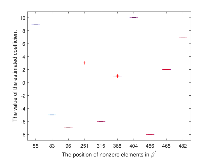
Figure 1: The calculation effect of SSNAL with $n=10000$, $p=500$, and $\lambda=0.5$.

The second task is to compare the performance of SSNAL and ADMM to solve the problem (3.3) with the using of standard lasso penalty and adaptive lasso penalty. The corresponding algorithms are named SSNAL_a, SSNAL_l, ADMM_a and ADMM_l, respectively. In this test, the true coefficient $\beta^{*}$ is generated by setting the values of the some components to be uniformly distributed in an interval, while the values of others are zero. The fixed interval is $[0,20]$ and the number of non-zeros of $\beta^{*}$ is set $20$. For model (1.1), the number of samples is set as $n=1000$ and the dimension is set as $p=500$. We run SSNAL and ADMM $20$ times to solve the problem (3.3) again and again, and the average results are listed in Table 1.

Table 1: Comparison results of SSNAL and ADMM with $n=1000$ and $p=500$.

Methods	ReErr	NNZ	Res	Time(s)	Iter
SSNALa	7.50e-3 (1.40e-3)	20 (0)	3.71e-8 (8.95e-9)	0.29 (0.07)	4 (0)
SSNALl	2.37e-2 (3.90e-3)	21.6 (1.51)	3.44e-8 (7.79e-9)	1.11 (0.20)	5 (0)
ADMMa	7.50e-3 (1.40e-3)	20 (0)	9.89e-7 (5.69e-9)	73.68 (6.88)	608.50 (23.38)
ADMMl	2.37e-2 (3.90e-3)	21.6 (1.51)	9.85-7 (5.35e-9)	70.84 (3.26)	604.40 (16.19)

We can see from this table that the $``\text{ReErr}"$ values derived by both methods using adaptive lasso are always lower than those using lasso. The methods using adaptive lasso can successfully select all the non-zero components, but the lasso cannot. This phenomena is consistent the famous theoretical results in the literature that the approach using adaptive lasso enjoys the desirable oracle properties. Besides, we see that both SSNAL and ADMM can successfully estimate the regression coefficient within a finite number of iterations in the sense that the termination criterion (5.10) is met. At last, it can be seen from the last two columns that the computing time and the number of iterations needed by SSNAL is greatly less than those by ADMM, which shows that the PLS method is effective and the SSNAL method is very progressive.

5.2.3 High-dimensional Case (p$>$n)

In this part, we generate a $p\times n$ random Gaussian matrix $\bar{X}$ whose entries are i.i.d. $\sim\mathcal{N}(0,1)$. Then the design matrix $X$ is generated by setting $X_{1}=\bar{X}_{1}$, $X_{n}=\bar{X}_{n}$, and $X_{j}=\bar{X}_{j}+0.7*(\bar{X}_{j+1}+\bar{X}_{j-1})$ for $j=2,\cdots,n-1$. Different to the lower-dimension case, the measurable function in model (1.1) is chosen as $g(x)=\cos(2\pi x)$ with $x\in[0,1]$.

The first task in this part is to illustrate the effectiveness of SSNAL in a high-dimensional case, say $n=300$ and $p=10000$. In this test, we consider the case where the underlying regression coefficient $\beta^{*}$ in model (1.1) only contains $10$ number of non-zero component with fixed position, that is $\beta^{*}_{i}=0$ except for $\beta^{*}_{104}=5$, $\beta^{*}_{572}=2$, $\beta^{*}_{1746}=-4$, $\beta^{*}_{2947}=-3$, $\beta^{*}_{4065}=-5$, $\beta^{*}_{5092}=4$, $\beta^{*}_{5112}=-1$, $\beta^{*}_{6680}=1$, $\beta^{*}_{7979}=-2$, and $\beta^{*}_{8460}=3$. The parameters’ values used in SSNAL and ADMM are set as the same as the test previously. Besides, we also run both algorithms $20$ times randomly and draw the box plot for the estimated coefficients in Figure 2. It can be seen clearly that the variables are selected correctly and their values are estimated are almost accurately. Hence, this simple test once again showS that SSNAL performs well in high-dimensional study.

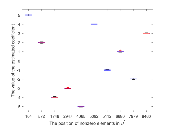
Figure 2: The calculation effect of SSNAL with $n=300$, $p=10000$ and $\lambda=0.1$.

The second task is to illustrate the numerical superiorities of SSNAL over ADMM using adaptive lasso and lasso penalty at high-dimensional case. In this test, we choose $n=500$ and $p=1000$, and set $a=5\sqrt{2\log(p)/n}$ and $b=100a$ to construct an interval such that there are $20$ nonzero elements of underlying regression coefficient $\beta^{*}$ uniformly distributed in this interval. As in the previous test, we run SSNAL and ADMM $20$ times to estimate this coefficient $\beta^{*}$, and the positions of these non-zero components are assigned randomly at each time. The average results regarding to ReErr, NNZ, Res, Time(s), and Iter are recorded in Table 2. From this table, we clearly see that SSNAL is highly efficient than ADMM in the sense of requiring much fewer computing time and much less iterations to derive the solutions with competitive accuracy.

Table 2: Average results of SSNAL and ADMM with $n=500$ and $p=1000$.

Methods	ReErr	NNZ	Res	Time(s)	Iter
SSNALa	7.03e-4 (1.10e-4)	20 (0)	2.60e-7 (2.24e-7)	0.06 (0.04)	1.7 (0.67)
SSNALl	2.90e-3 (6.15e-4)	19.9 (0.31)	1.34e-7 (2.93e-7)	0.53 (0.20)	4.9 (0.31)
ADMMa	7.03e-4 (1.10e-4)	20 (0)	9.97e-7 (2.49e-9)	52.37 (3.03)	955 (39.79)
ADMMl	2.90e-3 (6.00e-4)	20 (0)	9.94e-7 (3.56e-9)	51.43 (3.26)	944.7 (31.51)

5.3 Real Data Study

In this section, we further evaluate the effectiveness of PLS and the progressiveness of SSNAL by the using of the workers’ wage data which is available at https://rdrr.io/cran/ISLR/man/Wage.html. This data set contains the wage information of $3000$ male workers in the Mid-Atlantic region, as well as year, age, marriage status, race, education level, region, type of job, health level, health insurance information. Specifically, in this test, we don’t consider the data of year in which wage information was recorded and the logarithm of workers’ wage for the sake of simplicity. It should be noted that since only the Mid-Atlantic region is contained in this data, so the using of region indicator is unnecessary. We note that there should be a non-linear relationship between the education level and the wage, so the education level is set as variable $T$ in the non-parameter part $g(T)$ in (1.1). In this test, we consider $6$ covariates to relate the wage for each worker, say age, martial status, race, type of job, health level, and health insurance, which are denoted respectively as $X_{ij}$ from $j=1$ to $6$ for each worker $i$. More descriptions on each sample $X_{i}$ for index $j$ can be found at the second column of Table 3. For numerical convenience, we normalize all predictors with mean $0$ and variance $1$. Moreover, for the adaptive lasso penalized models, the way to generate the weights vector $\omega$ is the same as the one at the low-dimensional case tested previously. As before, we also use SSNAL and ADMM to solve the problem (3.3) to estimate the coefficient $\beta$ in model (1.1) by the using of lasso and adaptive lasso, respectively. The $\bar{\beta}$ estimated by SSNAL and ADMM with adaptive lasso penalty (named SSNALa and ADMMa) and lasso penalty (named SSNALl and ADMMl) are reported at the third to last column of Table 3. The numerical results of Res, NNZ, Iter, Time(s) are reported in bottom part of Table 3. It can be seen from these results that adaptive lasso penalized model can select $5$ covariates, while the lasso penalized model cannot, and SSNAL requires much less iterations and runs very faster than ADMM.

Table 3: Numerical results of SSNAL and ADMM on the $3000$ male workers’ wage.

Variable	Description	$\bar{\beta}$(SSNALa)	$\bar{\beta}$(SSNALl)	$\bar{\beta}$(ADMMa)	$\bar{\beta}$(ADMMl)
$X_{i1}$	Age of worker	5.9035	5.6215	5.9035	5.6215
$X_{i2}$	Marital status:	0	0.9409	0	0.9409
	(1=Never Married, 2=Married,
	3=Widowed, 4=Divorced,
	5=Separated)
$X_{i3}$	Race:	2.0303	2.1937	2.0303	2.1937
	(1=Other, 2=Black,
	3=Asian, 4=White)
$X_{i4}$	Type of job:	1.3296	1.6557	1.3296	1.6557
	(1=Industrial, 2=Information)
$X_{i5}$	Health level:	3.4366	3.4914	3.4366	3.4914
	(1=Good, 2=Very Good)
$X_{i6}$	Health insurance:	8.1894	8.1401	8.1894	8.1401
	(1=Yes, 0=No)
Res		4.86e-7	1.71e-7	9.75e-7	6.29e-7
NNZ		5	6	5	6
Iter		3	2	277	16
Time(s)		2.01	0.26	276.76	15.37

6 Conclusions

This paper concerned a partially linear semiparametric regression model with an unknown regression coefficient and an unknown nonparametric function. Specifically, we proposed a PLS method to estimate and select the regression coefficient. We showed that the oracle property of proposed PLS can be easily followed from some existing works in the literature. For practical implementation, this paper technically employed an efficient SSNAL method which is different to almost all the existing approaches in the sense that we targeted to the corresponding dual problem. What’s more, a semismooth Newton algorithm was used to solve the resulting strongly semismooth nonlinear system involved per-iteration by making full use of the structure of lasso. Finally, we tested the algorithm and did performance comparison with ADMM by using some random synthetic data and real data. The comparison results demonstrated that the PLS is very effective and the performance of the proposed SSNAL is highly efficient.

References

- Beck and Teboulle (2009) Beck, A. and M. Teboulle (2009). A Fast Iterative Shrinkage-Thresholding Algorithm for Linear Inverse Problems. SIAM Journal on Imaging Sciences 2(1), 183–202.
- Byrd et al. (2016) Byrd, R. H., G. M. Chin, J. Nocedal, et al. (2016). A Family of Second-Order Methods for Convex -Regularized Optimization. Mathematical Programming 159(1-2), 435–467.
- Clarke (1983) Clarke, F. H. (1983). Optimization and Nonsmooth Analysis. John Wiley and Sons.
- Engle et al. (1986) Engle, R. F., C. W. J. Granger, J. Rice, et al. (1986). Semiparametric Estimates of The Relation Between Weather and Electricity Sales. Journal of the American Statistical Association 81(394), 247–269.
- Fan and Gijbels (1996) Fan, J. Q. and I. Gijbels (1996). Local Polynomial Modelling and Its Applications. Monographs on Statistics and Applied Probability 66(1), Routledge. https://doi.org/10.1201/9780203748725.
- Fan and Li (2001) Fan, J. Q. and R. Li (2001). Variable Selection via Nonconcave Penalized Likelihood and Its Oracle Properties. Publications of the American Statistical Association 96(456), 1348–1360.
- Fan and Li (2004) Fan, J. Q. and R. Li (2004). New Estimation and Model Selection Procedures for Semiparametric Modeling in Longitudinal Data Analysis. Journal of the American Statistical Association 99, 710–723.
- Fan and Lv (2008) Fan, J. Q. and J. C. Lv (2008). Sure Independence Screening for Ultrahigh Dimensional Feature Space. Journal of the Royal Statistical Society: Series B (Statistical Methodology) 70(5), 849–911.
- Fazel et al. (2013) Fazel, M., T. K. Pong, D. F. Sun, et al. (2013). Hankel Matrix Rank Minimization with Applications in System Identification and Realization. SIAM Journal on Matrix Analysis and Applcations 34(3), 946–977.
- Goebel and Rockafellar (2008) Goebel, R. and R. T. Rockafellar (2008). Local Strong Convexity and Local Lipschitz Continuity of the Gradient of Convex Functions. Journal of Convex Analysis 15(2), 263–270.
- Golub and Loan (1996) Golub, G. H. and C. F. V. Loan (1996). Matrix Computations. Johns Hopkins University Press.
- Hardle et al. (2000) Hardle, W., H. Liang, and J. Gao (2000). Partially Linear Models. New-York: Springer-Verlag.
- Jiao et al. (2015) Jiao, Y. L., B. T. Jin, and X. L. Lu (2015). A Primal Dual Active Set with Continuation Algorithm for the -Regularized Optimization Problem. Applied Computational Harmonic Analysis 39(3), 400–426.
- Konishi and Kitagawa (2007) Konishi, S. and G. Kitagawa (2007). Information Criteria and Statistical Modeling. Berlin, Germany: Springer-Verlag.
- Li et al. (2008) Li, G. R., P. Tian, and L. G. Xue (2008). Generalized empirical likelihood inference in semiparametric regression model for longitudinal data. Acta Mathematica Sinica, English Series 24(12), 2029–2040.
- Li and Li (2012) Li, F., L. Y. Q. and G. R. Li (2012). Variable Selection for Partically Linear Models via Adaptive Lasso. Chinses Journal od Applied Probabbility and Statistics 28(6), 614–624.
- Li et al. (2016) Li, X. D., D. F. Sun, and K. C. Toh (2016). A Highly Efficient Semismooth Newton Augmented Lagrangian Method for Solving LASSO Problems. SIAM Journal on Optimization 28(1), 433–458.
- Liang and Li (2009) Liang, H. and R. Z. Li (2009). Variable Selection for Partially Linear Models with Measurement Errors. Journal of the American Statistical Association 104(485), 234–248.
- Lv and Fan (2009) Lv, J. C. and Y. Y. Fan (2009). A Unified Approach to Model Selection and Sparse Recovery using Regularized Least Squares. Annals of Statistics 37(6A), 3498–3528.
- Nesterov (1983) Nesterov, Y. (1983). A Method of Solving a Convex Programming Problem with Convergence Rate . Soviet Mathematics Doklady 27, 372–376.
- Ni et al. (2009) Ni, X., H. H. Zhang, and D. W. Zhang (2009). Automatic Model Selection for Partially Linear Models. Journal of Multivariate Analysis 100(9), 2100–2111.
- Rockafellar (1970) Rockafellar, R. T. (1970). Convex Analysis. Princeton University Press.
- Rockafellar (1976a) Rockafellar, R. T. (1976a). Augmented Lagrangians and Applications of the Proximal Point Algorithm in Convex Programming. Mathematics of Operations Research 1, 97–116.
- Rockafellar (1976b) Rockafellar, R. T. (1976b). Monotone Operators and the Proximal Point Algorithm. SIAM Journal on Control and Optimization 14(5), 877–898.
- Rockafellar and Wets (1998) Rockafellar, R. T. and R. J.-B. Wets (1998). Variational Analysis. Grundlehren der mathematischen Wissenschaften.
- Speckman (1988) Speckman, P. (1988). Kernel Smoothing in Partial Lineal Models. Journal of the Royal Statistical Society: Series B 50(3), 413–436.
- Stigler (1981) Stigler, S. M. (1981). Gauss and the Invention of Least Squares. Annals of Statistics 9(3), 465–474.
- Tibshirani (1996) Tibshirani, R. (1996). Regression Shrinkage and Selection via the Lasso. Journal of the Royal Statistical Society: Series B 58(1), 267–288.
- Tibshirani et al. (2005) Tibshirani, R., M. Saunders, S. Rosset, et al. (2005). Sparsity and Smoothness via the Fused Lasso. Journal of the Royal Statistical Society: Series B 67(1), 91–108.
- Wang et al. (2007) Wang, H. S., R. Z. Li, and C. L. Tsai (2007). Tuning Parameter Selectors for the Smoothly Clipped Absolute Deviation Method. Biometrika 94(3), 553–568.
- Wang et al. (2013) Wang, L., Y. D. Kim, and R. Z. Li (2013). Calibrating Nonconvex Penalized Regression in Ultra-high Dimension. Annals of Statistics 41(5), 2505–2536.
- Wang and Jing (2003) Wang, Q. H. and B. Y. Jing (2003). Empirical likelihood for partial linear models. Annals of the Institute of Statistical Mathematics 55(3), 585–595.
- Xie and Huang (2009) Xie, H. L. and J. Huang (2009). SCAD-penalized Regression in High-dimensional Partially Linear Models. Annals of Statistics 37, 673–696.
- Zou (2006) Zou, H. (2006). The Adaptive Lasso and Its Oracle Properties. Journal of the American Statistical Association 101(476), 1418–1429.