An OSRC Preconditioner for the EFIE

Abstract

The Electric Field Integral Equation (EFIE) is a well-established tool to solve electromagnetic scattering problems. However, the development of efficient and easy to implement preconditioners remains an active research area. In recent years, operator preconditioning approaches have become popular for the EFIE, where the electric field boundary integral operator is regularised by multiplication with another convenient operator. A particularly intriguing choice is the exact Magnetic-to-Electric (MtE) operator as regulariser. But, evaluating this operator is as expensive as solving the original EFIE. In work by El Bouajaji, Antoine and Geuzaine, approximate local Magnetic-to-Electric surface operators for the time-harmonic Maxwell equation were proposed. These can be efficiently evaluated through the solution of sparse problems. This paper demonstrates the preconditioning properties of these approximate MtE operators for the EFIE. The implementation is described and a number of numerical comparisons against other preconditioning techniques for the EFIE are presented to demonstrate the effectiveness of this new technique.

Keywords Preconditioner, OSRC approximation, Electric Field Integral Equation.

1 Introduction

The numerical simulation of time-harmonic waves scattered by perfect electric conductors (PECs) is of fundamental importance across the spectrum of electromagnetic applications.

Denote by $\mathbf{e}^{\textup{inc}}$ an incident field. We are looking for the solution $\mathbf{e}^{\textup{tot}}=\mathbf{e}^{\textup{inc}}+\mathbf{e}^{\textup{scat}}$ of the exterior scattering problem, that satisfies:

$$\textup{{curl}}\,\textup{{curl}}\,\mathbf{e}^{\textup{tot}}-\kappa^{2}\mathbf{e}^{\textup{tot}} =0 \text{in }\Omega^{\textup{+}},$$ (1a)

$$\mathbf{e}^{\textup{tot}}\times\boldsymbol{\nu} =0 \text{on }\Gamma,$$ (1b)

$$\lim_{|\mathbf{x}|\rightarrow\infty}|\mathbf{x}|\left(\textup{{curl}}\,\mathbf{e}^{\textup{scat}}\times\frac{\mathbf{x}}{|\mathbf{x}|}-\mathrm{i}\kappa\mathbf{e}^{\textup{scat}}\right) =0.$$ (1c)

Here, $\kappa=\omega\sqrt{\epsilon_{0}\mu_{0}}$ denotes the wavenumber of the problem, with $\omega$ denoting the frequency and $\epsilon_{0}$ and $\mu_{0}$ the electric permittivity and magnetic permeability in vacuum. The PEC object is denoted by $\Omega^{-}\subset\mathbb{R}^{3}$ and it is enclosed by a smooth boundary $\Gamma=\delta\Omega^{-}$, also $\Omega^{+}=\mathbb{R}^{3}\setminus\overline{\Omega^{-}}$ denotes the propagation medium. Frequently, the incident field is a plane wave given by $\mathbf{e}^{\textup{inc}}=\mathbf{p}\mathrm{e}^{\mathrm{i}\kappa\mathbf{x}\cdot\mathbf{d}}$, where $\mathbf{p}$ is a non-zero vector representing the polarisation of the wave, $\mathbf{d}$ is a unit vector perpendicular to $\mathbf{p}$ that gives the direction of the plane wave and $\boldsymbol{\nu}$ denotes the unit normal vector which is orthogonal to the local tangent plane to the surface of the scatterer.

An integral equation formulation of this problem leads to an operational equation of the form

$$\begin{split}\mathbf{S}_{\kappa}\mathbf{u}=-\left(\frac{\mathbf{I}}{2}+\mathbf{C}_{\kappa}\right)\mathbf{f},\end{split}$$ (2)

with $\mathbf{S}_{\kappa}$ the electric field integral operator, $\mathbf{C}_{\kappa}$ the magnetic field integral operator, $\mathbf{f}$ the tangential trace of the incident data and $\mathbf{u}$ the solution to the system (we will define all these quantities in Section 2.3). The above is a direct formulation, but one could equally choose an indirect formulation. See [9] for details.

For moderate mesh sizes, the discretisation of (2) can easily be solved by LU decomposition. As the mesh width decreases, iterative solvers become necessary though, but are hampered by the ill-conditioning of $\mathbf{S}_{\kappa}$ after discretisation. A strategy to deal with this issue is to introduce a regularisation operator $\mathbf{R}$ such that the new operator system,

$$\begin{split}\mathbf{R}\mathbf{S}_{\kappa}\mathbf{u}=-\mathbf{R}\left(\frac{\mathbf{I}}{2}+\mathbf{C}_{\kappa}\right)\mathbf{f},\end{split}$$ (3)

leads to well-conditioned discretisations.

The most common example of $\mathbf{R}$ is the Calderón Multiplicative Preconditioner [2]. The drawback of this method, however, is the need to evaluate discrete operator products. To illustrate this, assume a function $\phi$ in some Hilbert space, and operators $\mathbf{A}$ and $\mathbf{B}$ in compatible Hilbert spaces. In order to evaluate the product $\psi=\mathbf{AB}\phi$ through Galerkin discretisations of the operators $\mathbf{A}$ and $\mathbf{B}$, we need to compute a finite dimensional matrix product of the form $\psi_{h}=\mathbf{A}_{h}\mathbf{M}_{h}^{-1}\mathbf{B}_{h}\phi_{h},$ where we have used the subscript _h to denote finite dimensional quantities after discretisation [5]. The matrix $\mathbf{M}_{h}$ is a mass matrix, which contains the inner product of the test space of $\mathbf{B}_{h}$ and the domain space of $\mathbf{A}_{h}$. The difficulty is that this mass matrix is numerically singular for the standard choice of Rao-Wilton-Glisson (RWG) basis functions in electromagnetic scattering [7]. In order to overcome this problem, one can use the so-called Buffa-Christiansen (BC) bases as the range space of the EFIE operator [2]. However, their use is expensive, since the construction of BC functions requires barycentric mesh refinements (see Fig. 1 for reference).

Figure 1: Primal and barycentric (dashed lines) meshes.

The thrust of this paper is to use the Magnetic-to-Electric (MtE) operator, while avoiding expensive barycentric mesh refinements. With this choice, the left-hand side of (3) becomes a second kind integral operator, which in theory, will make it more amenable to iterative solvers. However, a direct evaluation of the MtE operator has a similar complexity to solving the original scattering problem and is, therefore, impractical. The idea of the On-Surface-Radiation-Condition (OSRC) approach [15] is to obtain a high frequency approximation of the MtE operator from a radiation condition applied on the surface of the scatterer.

In recent work by Bouajaji, Antoine, and Geuzaine [11], the authors approximated the high-frequency symbol of the MtE operator by a Padé expansion [16] that can be discretised using sparse surface operators and thereby, be efficiently evaluated. Earlier work in the 2D electromagnetic and acoustic cases is included in [4, 3, 10].

In this research we follow the aforementioned approach for approximating the MtE operator and investigate its practical suitability as a regulariser for the EFIE. We also demonstrate details of the implementation and the resulting preconditioning performance, with respect to assembly and solving times.

This paper is organised as follows: in section 2 an overview of function spaces for Maxwell’s boundary integral operators is presented. Section 3 shows the MtE preconditioner, its continuous implementation, approximations, its discrete implementation and simplifications connsidered. Section 4 presents a validation of this preconditioner and performance benchmarks, with concluding remarks in Section 5.

2 Problem setting, Tangential Sobolev Spaces and Surface Operators

We will start by introducing some required surface differential operators for the later sections. We will then discuss the function space setting and the discrete representation. Finally, we will introduce the required boundary operators.

2.1 Surface differential operators

In this section we briefly introduce the required surface differential operators. For a more complete technical definition see e.g. [17]. For the sake of the definitions here we assume a smooth bounded domain $\Omega$ with sufficiently smooth boundary $\Gamma$.

Let $u$ be a sufficiently smooth scalar vector field defined on $\Gamma$ and $\mathbf{v}$ a sufficiently smooth tangential vector field defined on $\Gamma$, that is $\mathbf{v}\cdot\boldsymbol{\nu}=0$. Furthermore, denote by $\tilde{u}$ and $\tilde{\mathbf{v}}$ suitable extensions into a neighbourhood $\Gamma_{\epsilon}$ of $\Gamma$ with $\mathbf{\tilde{v}}$ also requiring that it is tangential to surfaces in $\Gamma_{\epsilon}$ parallel to $\Gamma$. We define the following operators.

• The surface gradient

  $$\mathbf{Grad}_{\Gamma}:=\nabla\tilde{u}|_{\Gamma}.$$

• The tangential curl

  $$\mathbf{curl}_{\Gamma}:=\mathbf{Grad}_{\Gamma}u\times\boldsymbol{\nu}.$$

• The surface divergence

  $$\mathbf{Div}_{\Gamma}\;\mathbf{v}:=(\text{div}\;\tilde{\mathbf{v}})|_{\Gamma}.$$

• The surface curl

  $$\text{curl}_{\Gamma}\;\mathbf{v}:=\boldsymbol{\nu}\cdot(\text{curl}\;\tilde{\mathbf{v}})|_{\Gamma}.$$

We have the following identities (see [17, Theorem 2.5.19])

$$\int_{\Gamma}\mathbf{Grad}_{\Gamma}u\cdot\mathbf{v}\;d\Gamma =-\int_{\Gamma}u\,\mathbf{Div}_{\Gamma}\,\mathbf{v}\;d\Gamma,$$

$$\int_{\Gamma}\left(\mathbf{curl}_{\Gamma}\,u\cdot\mathbf{v}\right)d\Gamma =\int_{\Gamma}u\,\text{curl}_{\Gamma}\mathbf{v}\,d\Gamma,$$

$$\mathbf{Div}_{\Gamma}\,\mathbf{curl}_{\Gamma}\,u =0,$$

$$\text{curl}_{\Gamma}\mathbf{Grad}_{\Gamma}u =0,$$

$$\mathbf{Div}_{\Gamma}\,(\mathbf{v}\times\boldsymbol{\nu}) =\text{curl}_{\Gamma}\,\mathbf{v}.$$

Moreover, we can define the scalar surface Laplace operator as

$$\Delta_{\Gamma}u:=\mathbf{Div}_{\Gamma}\;\mathbf{Grad}_{\Gamma}u=-\text{curl}_{\Gamma}\;\mathbf{curl}_{\Gamma}u,$$

and the vectorial surface Laplace operator as

$$\Delta_{\Gamma}\mathbf{v}:=\mathbf{Grad}_{\Gamma}\;\mathbf{Div}_{\Gamma}\mathbf{v}-\mathbf{curl}_{\Gamma}\;\text{curl}_{\Gamma}\mathbf{v}$$

(see [17, 2.5.191 & 2.5.192]).

2.2 Function Spaces

Consider sufficiently smooth vector fields $\mathbf{u}$ and $\mathbf{v}$ such that the following implication of Green’s formula makes sense:

$$\int_{\Omega}(\mathbf{u}\cdot\textbf{curl}\;\mathbf{v}-\mathbf{v}\cdot\textbf{curl}\;\mathbf{u})\;d\Omega=\int_{\Gamma}\gamma_{t}\mathbf{u}\cdot\mathbf{v}|_{\Gamma}\;d\Gamma.$$ (4)

The operator $\gamma_{t}\mathbf{u}$ is the tangential trace: the product $\mathbf{u}\times\boldsymbol{\nu}$ taken on the boundary $\Gamma$.

Now define the tangential component trace $\pi_{t}$ as

$$\pi_{t}\mathbf{v}:=\mathbf{v}-(\boldsymbol{\nu}\cdot{\mathbf{v}})\boldsymbol{\nu}=\boldsymbol{\nu}\times(\gamma_{t}\mathbf{v})$$

on $\Gamma$.

Equation (4) introduces a duality relationship between $\gamma_{t}$ and $\pi_{t}$, since

$$\int_{\Gamma}\gamma_{t}\mathbf{u}\cdot\mathbf{v}|_{\Gamma}\;d\Gamma=\int_{\Gamma}\gamma_{t}\mathbf{u}\cdot\pi_{t}\mathbf{v}\;d\Gamma.$$

Moreover, the same formula motivates a self-duality for tangential traces through

$$\int_{\Gamma}\gamma_{t}\mathbf{u}\cdot\pi_{t}\mathbf{v}\;d\Gamma=\int_{\Gamma}\gamma_{t}\mathbf{u}\cdot(\boldsymbol{\nu}\times\gamma_{t}\mathbf{v})\;d\Gamma=:\langle\gamma_{t}\mathbf{u},\gamma_{t}\mathbf{v}\rangle_{\times}.$$

From (4) it follows that the dual form $\langle\cdot,\cdot\rangle_{\times}$ makes sense for tangential traces of functions whose curl is well defined.

In the early 2000s the underlying ideas were made precise in the context of Sobolev spaces on bounded Lipschitz domains (see [6, 8]). A beautiful summary is also given in the overview paper [9].

Here, we just summarise the key result with respect to the trace of $\gamma_{t}$ and the dual form $\langle\cdot,\cdot\rangle_{\times}$.

Let $\Omega$ be bounded (the case of an unbounded domain is similar). Define

$$\mathbf{H}^{s}(\mathbf{curl},\Omega):=\{\mathbf{u}\in\mathbf{H}^{s}(\Omega)|\;\mathbf{curl}\;\mathbf{u}\in\mathbf{H}^{s}(\Omega)\}$$

as the usual space for weak solutions of Maxwell’s equations. In the following, we will denote $\mathbf{H}=\mathbf{H}^{0}$. Then, one can define the space $\mathbf{H}_{\times}^{-\frac{1}{2}}(\textbf{Div}_{\Gamma},\Gamma)$ of tangential traces on the boundary such that the mapping $\gamma_{t}:\mathbf{H}(\mathbf{curl},\Omega)\rightarrow\mathbf{H}_{\times}^{-\frac{1}{2}}(\textbf{Div}_{\Gamma},\Gamma)$ is continuous and surjective. Moreover, this space is self-dual with respect to the dual form $\langle\cdot,\cdot\rangle_{\times}$ [9]. Correspondingly, we introduce the space $\mathbf{H}_{\times}^{-\frac{1}{2}}(\text{curl}_{\Gamma},\Gamma)$ as the continuous and surjective range of the map $\pi_{t}:\mathbf{H}(\mathbf{curl},\Omega)\rightarrow\mathbf{H}_{\times}^{-\frac{1}{2}}(\text{curl}_{\Gamma},\Gamma)$. There is an isomorphism $\boldsymbol{\Theta}:\mathbf{H}_{\times}^{-\frac{1}{2}}(\textbf{Div}_{\Gamma},\Gamma)\rightarrow\mathbf{H}_{\times}^{-\frac{1}{2}}(\text{curl}_{\Gamma},\Gamma)$ whose geometric interpretation on smooth boundaries is that $\boldsymbol{\nu}\times\phi=\psi$ for some $\phi\in\mathbf{H}_{\times}^{-\frac{1}{2}}(\textbf{Div}_{\Gamma},\Gamma)$ and $\psi\in\mathbf{H}_{\times}^{-\frac{1}{2}}(\text{curl}_{\Gamma},\Gamma)$. The notations $\mathbf{Div}_{\Gamma}$ and $\text{curl}_{\Gamma}$ in the names of the spaces make clear that they are weakly surface div and surface curl conforming, respectively. For precise definitions see [8].

We will also require the usual scalar surface spaces $H^{1/2}(\Gamma)$ and $H^{-1/2}(\Gamma)$. The former can be interpreted as space of scalar Dirichlet data and the latter as space of scalar (weak) normal derivatives. For all traces jumps and average operators can be defined as

$$\left[\gamma\right]_{\Gamma} =\gamma^{+}-\gamma^{-}$$

$$\left\{\gamma\right\}_{\Gamma} =\frac{\gamma^{+}+\gamma^{-}}{2}$$

In order to build the discrete problem, we need to define discrete representations of $\mathbf{H}_{\times}^{-\frac{1}{2}}(\textbf{Div}_{\Gamma},\Gamma)$ and $\mathbf{H}_{\times}^{-\frac{1}{2}}(\text{curl}_{\Gamma},\Gamma)$.

Consider a polyhedral approximation $\Gamma_{h}$ of $\Gamma$ with a triangulation $\mathcal{T}_{h}=\cup_{l=1}^{N_{T}}T^{l}$, we denominate as Raviart-Thomas (RT) the space of linear edge finite elements defined by the basis functions

Figure 2: Definition of a RT basis function on an edge of the mesh

$$\mathbf{RT}_{i}(\mathbf{x})=\begin{cases}\frac{1}{2A_{i}^{+}}(\mathbf{x}-\mathbf{p}_{+})\;\;\text{ if }\mathbf{x}\in T_{+}\\ -\frac{1}{2A_{i}^{-}}(\mathbf{x}-\mathbf{p}_{-})\text{ if }\mathbf{x}\in T_{-}\\ \mathbf{0}\text{, otherwise }\end{cases},\;\;i\in\left\{1,\dots,N_{e}\right\}$$

(see, for example, Fig. 2), where $N_{e}$ is the number of edges in $\mathcal{T}_{h}$.

We define Nédélec (NC) basis functions as the set of rotated RT basis functions:

$$\mathbf{NC}_{i}:=\boldsymbol{\nu}(\mathbf{x})\times\mathbf{RT}_{i}(\mathbf{x})$$

The RT and NC basis functions form discrete bases of the dual pair $\mathbf{H}_{\times}^{-\frac{1}{2}}(\textbf{Div}_{\Gamma},\Gamma)$ and $\mathbf{H}_{\times}^{-\frac{1}{2}}(\text{curl}_{\Gamma},\Gamma)$.

We also define the Rao-Wilton-Glisson (RWG) basis functions ([19]) as a scaling of RT basis functions:

$$\mathbf{RWG}_{i}:=l_{i}\mathbf{RT}_{i}(\mathbf{x}),$$

where $l_{i}$ is the length of the edge $i$ and the Scaled Nédélec (SNC) basis functions as the rotation of RWG:

$$\mathbf{SNC}_{i}:=\boldsymbol{\nu}(\mathbf{x})\times\mathbf{RWG}_{i}(\mathbf{x})$$

Just like the pair RT-NC, RWG and SNC form discrete bases of the dual pair $\mathbf{H}_{\times}^{-\frac{1}{2}}(\textbf{Div}_{\Gamma},\Gamma)$ and $\mathbf{H}_{\times}^{-\frac{1}{2}}(\text{curl}_{\Gamma},\Gamma)$.

Finally, we define piecewise linear basis functions (P1) on a reference element:

$$f_{i}(\xi,\eta)=\begin{cases}1-\xi-\eta&\text{ for vertex 1}\\ \xi&\text{ for vertex 2}\\ \eta&\text{ for vertex 3}\end{cases},\;\;i\in\left\{1,\dots,N_{v}\right\},$$

where $N_{v}$ is the number of vertices in $\mathcal{T}_{h}$. These are also called roof basis functions; we intend to use them to discretise $H^{\frac{1}{2}}(\Gamma)$ and $H^{-\frac{1}{2}}(\Gamma)$ in the upcoming sections.

In table 1 we summarise the notation used for the different sets of basis functions.

Acronym	Type	Dofs	Discretises
RT	Vectorial	Edges	$\mathbf{H}_{\times}^{-\frac{1}{2}}(\textbf{Div}_{\Gamma},\Gamma)$
NC	Vectorial	Edges	$\mathbf{H}_{\times}^{-\frac{1}{2}}(\text{curl}_{\Gamma},\Gamma)$
RWG	Vectorial	Edges	$\mathbf{H}_{\times}^{-\frac{1}{2}}(\textbf{Div}_{\Gamma},\Gamma)$
SNC	Vectorial	Edges	$\mathbf{H}_{\times}^{-\frac{1}{2}}(\text{curl}_{\Gamma},\Gamma)$
P1	Scalar	Vertices	$H^{\frac{1}{2}}(\Gamma)$ and $H^{-\frac{1}{2}}(\Gamma)$

Table 1: Summary of basis functions.

2.3 Operators

To solve (1a)-(1c), the Stratton-Chu representation formula [14, Theorem 3.27] must be considered for any $\mathbf{x}\in\Omega^{+}$

$$\mathbf{e}(\mathbf{x}):=-\mathcal{T}(\gamma_{N}^{+}\mathbf{e})(\mathbf{x})-\mathcal{K}(\gamma_{t}^{+}\mathbf{e})(\mathbf{x}).$$ (5)

Here $\gamma_{t}^{+}\mathbf{e}$ in physical terms represents the surface magnetic current and consequently, $\gamma_{N}^{+}\mathbf{e}$ is the surface electric current [18, equation (2.336)], defined by $\gamma_{N}^{+}\mathbf{u}:=(i\kappa)^{-1}{{\gamma_{t}}^{+}\textbf{curl}\;\mathbf{u}}$ (and similarly for the interior magnetic trace). $\mathcal{T},\mathcal{K}:\mathbf{H}_{\times}^{-\frac{1}{2}}(\textbf{Div}_{\Gamma},\Gamma)\rightarrow\mathbf{H}_{loc}(\textbf{curl}^{2},\Omega^{+})$ are defined as:

$$\mathcal{T}(\mathbf{p})(\mathbf{x}) :=i\kappa\int_{\Gamma}\mathbf{p}(\mathbf{y})\mathbf{G}(\mathbf{x},\mathbf{y})$$

$$-\frac{1}{i\kappa}\nabla_{\mathbf{x}}\int_{\Gamma}\mathbf{G}(\mathbf{x},\mathbf{y})\textbf{Div}_{\Gamma}\mathbf{p}(\mathbf{y})d\Gamma(\mathbf{y}),$$

$$\mathcal{K}(\mathbf{p})(\mathbf{x}) :=\textbf{curl}_{\mathbf{x}}\int_{\Gamma}\mathbf{G}(\mathbf{x},\mathbf{y})\mathbf{p}(\mathbf{y})d\Gamma(\mathbf{y})$$

With $\mathbf{G}(\mathbf{x},\mathbf{y}):=\frac{e^{i\kappa\left\|\mathbf{x}-\mathbf{y}\right\|}}{4\pi\left\|\mathbf{x}-\mathbf{y}\right\|}$, $\mathbf{x}\neq\mathbf{y}$.

By applying magnetic and tangential traces to the Electric and Magnetic field potential operators, the electric and magnetic BIOs (Boundary Integral Operators) $\mathbf{S}_{\kappa},\mathbf{C}_{\kappa}:\mathbf{H}_{\times}^{-\frac{1}{2}}(\textbf{Div}_{\Gamma},\Gamma)\rightarrow\mathbf{H}_{\times}^{-\frac{1}{2}}(\textbf{Div}_{\Gamma},\Gamma)$ can be obtained:

$$\{\gamma_{t}\}_{\Gamma}\mathcal{T} =\mathbf{S}_{\kappa} \left[\gamma_{t}\right]_{\Gamma}\mathcal{T} =0$$

$$\{\gamma_{t}\}_{\Gamma}\mathcal{K} =\mathbf{C}_{\kappa} \left[\gamma_{t}\right]_{\Gamma}\mathcal{K} =-\mathbf{I}$$

$$\{\gamma_{N}\}_{\Gamma}\mathcal{T} =\mathbf{C}_{\kappa} \left[\gamma_{N}\right]_{\Gamma}\mathcal{T} =-\mathbf{I}$$

$$\{\gamma_{N}\}_{\Gamma}\mathcal{K} =-\mathbf{S}_{\kappa} \left[\gamma_{N}\right]_{\Gamma}\mathcal{K} =0$$

$$\gamma_{t}^{-}\mathcal{T} =\mathbf{S}_{\kappa} \gamma_{t}^{+}\mathcal{T} =\mathbf{S}_{\kappa}$$

$$\gamma_{t}^{-}\mathcal{K} =\frac{\mathbf{I}}{2}+\mathbf{C}_{\kappa} \gamma_{t}^{+}\mathcal{K} =-\frac{\mathbf{I}}{2}+\mathbf{C}_{\kappa}$$

$$\gamma_{N}^{-}\mathcal{T} =\frac{\mathbf{I}}{2}+\mathbf{C}_{\kappa} \gamma_{N}^{+}\mathcal{T} =-\frac{\mathbf{I}}{2}+\mathbf{C}_{\kappa}$$

$$\gamma_{N}^{-}\mathcal{K} =-\mathbf{S}_{\kappa} \gamma_{N}^{+}\mathcal{K} =-\mathbf{S}_{\kappa}$$

Then, applying electric and magnetic traces to the representation formula (5), the following can be derived:

$$\mathcal{C}^{\pm}=\begin{bmatrix}\frac{\mathbf{I}}{2}\mp\mathbf{C}_{\kappa}&\mp\mathbf{S}_{\kappa}\\ \pm\mathbf{S}_{\kappa}&\frac{\mathbf{I}}{2}\mp\mathbf{C}_{\kappa}\\ \end{bmatrix}\begin{bmatrix}\gamma_{t}^{\pm}\mathbf{u}\\ \gamma_{N}^{\pm}\mathbf{u}\\ \end{bmatrix}=\begin{bmatrix}\gamma_{t}^{\pm}\mathbf{u}\\ \gamma_{N}^{\pm}\mathbf{u}\\ \end{bmatrix}.$$ (6)

The operator $\mathcal{C}^{\pm}$ is called Calderón Projector. It describes the relationship of the electric and magnetic tangential traces on the boundary $\Gamma$. An important property, directly following from the Stratton-Chu representation formula is that $\left(\mathcal{C}^{\pm}\right)^{2}=\mathcal{C}^{\pm}$, which implies

$$\mathbf{S}_{\kappa}^{2}=\mathbf{C}_{\kappa}^{2}-\frac{\mathbf{I}}{4}.$$ (7)

This is the basis for Calderón Preconditioning. It states that $\mathbf{S}_{\kappa}^{2}$ is a compact perturbation of the identity on sufficiently smooth domains, with eigenvalues clustering around the point $1/4$. Hence, under a suitable discretisation of this operator, iterative solvers are expected to converge quickly. The difficulties of building the discrete version arise when trying to build Gram matrices $\mathbf{G}$ to implement the discrete product $\mathbf{S}_{\kappa,h}\mathbf{G}^{-1}\mathbf{S}_{\kappa,h}$. For standard RWG spaces, the matrix $\mathbf{G}$ is singular [2]. To overcome this problem, in [2] a Calderón multiplicative preconditioner (CMP) was proposed based on the use of BC basis functions that are defined on barycentric refinements of the original grid (see [7] for more details and Fig. 1 for reference). While the improvement in iterative solver convergence with this preconditioner is excellent, the implementation requires the assembly of operators on grids with six times as many elements as the original grid. Acceleration techniques such as the Fast Multipole Method (FMM) [12] make this more manageable. Still, this is significantly more costly than the assembly on the original grid.

A recent approach to implement a Calderón Preconditioner is shown in [1], where the authors aim to build a Multiplicative Calderón Preconditioner immune to the low frequency breakdown induced by the use of RWG basis functions. Here, the authors perform a quasi-Helmholtz decomposition of the EFIE in the static limit by using loop-star basis functions [21] obtained from linear combinations of RWG basis functions, thus avoiding BC basis functions.

The main drawback of this technique, however, is the need to solve a dense matrix system as part of the application of the preconditioner. The authors have pointed out that this can be achieved by preconditioning this dense matrix with specific methods, making it competitive with the original CMP. However, the implementation effort of this approach is substantial. In this paper we demonstrate that OSRC based preconditioners achieve similar performance, without requiring barycentric refinements and with an implementation that only requires the solution of sparse linear systems that are straightforward to assemble.

3 Construction of an OSRC Preconditioner

We start by reviewing the preconditioning properties the EtM (Electric-to-Magnetic) operator $\mathbf{V}$ and its inverse: the MtE operator $\mathbf{V}^{-1}$. Then, we review the Padé approximation approach for these operators, obtained from [11], and finally describe in detail how to use these operators as discrete preconditioners. We assume that both $\mathbf{S}_{\kappa}$ and $\frac{1}{2}\mathbf{I}+\mathbf{C}_{\kappa}$ are invertible (the operators have no resonance at the wavenumber $\kappa$).

3.1 OSRC operator as a preconditioner for the EFIE

The EtM operator can be derived from the first row of (6)

$$-\mathbf{S}_{\kappa}^{-1}\left(\frac{\mathbf{I}}{2}+\mathbf{C}_{\kappa}\right)\gamma_{t}^{+}\mathbf{u}=\gamma_{N}^{+}\mathbf{u}.$$

Hence, the EtM and its inverse, the MtE operator, are given by:

$$\mathbf{V}_{(1)}=-\mathbf{S}_{\kappa}^{-1}\left(\frac{\mathbf{I}}{2}+\mathbf{C}_{\kappa}\right),$$ (8)

$$\mathbf{V}_{(1)}^{-1}=-\left(\frac{\mathbf{I}}{2}+\mathbf{C}_{\kappa}\right)^{-1}\mathbf{S}_{\kappa}.$$ (9)

Alternatively, from the second row of (6)

$$\left(\frac{\mathbf{I}}{2}+\mathbf{C}_{\kappa}\right)^{-1}\mathbf{S}_{\kappa}\gamma_{t}^{+}\mathbf{u}=\gamma_{N}^{+}\mathbf{u}.$$

A second version of the EtM exact operator and its inverse (MtE) can be obtained:

$$\mathbf{V}_{(2)}=\left(\frac{\mathbf{I}}{2}+\mathbf{C}_{\kappa}\right)^{-1}\mathbf{S}_{\kappa},$$ (10)

$$\mathbf{V}_{(2)}^{-1}=\mathbf{S}_{\kappa}^{-1}\left(\frac{\mathbf{I}}{2}+\mathbf{C}_{\kappa}\right).$$ (11)

It is necessary to remark that the discrete versions of the pairs (8), (11) and (9), (10) are not necessarily the same, since they might be defined on different discrete spaces. See [20] for details.

To discriminate versions of the $\mathbf{V}^{-1}$ operator, we have used the subscripts ₍₁₎ and ₍₂₎.

Theorem 1.

Assume that $\mathbf{V}_{(1)}$ and $\mathbf{V}_{(2)}$ and their inverses exist as defined above. It holds that

$$\mathbf{S}_{\kappa}\mathbf{V}^{-1}_{(2)}\equiv\left(\frac{\mathbf{I}}{2}+\mathbf{C}_{\kappa}\right)$$

and

$$\mathbf{V}^{-1}_{(1)}\mathbf{S}_{\kappa}\equiv\left(\frac{\mathbf{I}}{2}-\mathbf{C}_{\kappa}\right).$$

Proof.

The first relationship follows from

$$\mathbf{S}_{\kappa}\mathbf{V}^{-1}_{(2)}=\mathbf{S}_{\kappa}\mathbf{S}_{\kappa}^{-1}\left(\frac{\mathbf{I}}{2}+\mathbf{C}_{\kappa}\right)=\left(\frac{\mathbf{I}}{2}+\mathbf{C}_{\kappa}\right)$$

For the second identity we obtain

$$\mathbf{V}_{(1)}^{-1}\mathbf{S}_{\kappa}=-\left(\frac{\mathbf{I}}{2}+\mathbf{C}_{\kappa}\right)^{-1}\mathbf{S}_{\kappa}\mathbf{S}_{\kappa}.$$

To obtain the desired result we use (7) and replace $\mathbf{S}_{\kappa}^{2}=-\left(\frac{\mathbf{I}}{2}+\mathbf{C}_{\kappa}\right)\left(\frac{\mathbf{I}}{2}-\mathbf{C}_{\kappa}\right)$.

∎

It follows that on sufficiently smooth domains applying $\mathbf{V}_{(1)}^{-1}$ or $\mathbf{V}_{(2)}^{-1}$ from the left/right to $\mathbf{S}_{\kappa}$, respectively, results in a compact perturbation of the identity.

From now on, we drop the subscripts, and we refer to $\mathbf{V}_{(1)}^{-1}$ just as $\mathbf{V}^{-1}$.

We have seen that $\mathbf{V}^{-1}$ is a good candidate for a preconditioner. However, the construction of $\mathbf{V}^{-1}$ is as expensive as solving the EFIE, so finding a good approximation is essential.

3.2 Approximation of the MtE operator

In [11], it is shown that an approximation for the EtM on smooth surfaces is given by [11]

$$\gamma_{N}^{+}\mathbf{u}\approx-\boldsymbol{\Lambda}_{1,\varepsilon}^{-1}\boldsymbol{\Lambda}_{2,\varepsilon}(\boldsymbol{\nu}\times\gamma_{t}^{+}\mathbf{u})=-\boldsymbol{\Lambda}_{1,\varepsilon}^{-1}\boldsymbol{\Lambda}_{2,\varepsilon}\boldsymbol{\Theta}\gamma_{t}^{+}\mathbf{u}\;\;\text{ on }\Gamma,$$ (12)

where

$$\boldsymbol{\Lambda}_{2,\varepsilon}:=\mathbf{I}-\textbf{curl}_{\Gamma}\frac{1}{\kappa^{2}_{\varepsilon}}\text{curl}_{\Gamma},$$

and

$$\boldsymbol{\Lambda}_{1,\varepsilon}:=(\mathbf{I}+\mathcal{J})^{1/2},$$

with

$$\mathcal{J}:=\textbf{Grad}_{\Gamma}\frac{1}{\kappa^{2}_{\varepsilon}}\textbf{Div}_{\Gamma}-\textbf{curl}_{\Gamma}\frac{1}{\kappa^{2}_{\varepsilon}}\text{curl}_{\Gamma}.$$ (13)

Notice here that we have used the term $\kappa_{\varepsilon}=\kappa+i\varepsilon$ instead of $\kappa$. The term $\varepsilon>0$ is a damping parameter used by the authors in [11] to avoid singularities in the square root operator, whose optimal value is given by $\varepsilon=0.39\kappa^{\frac{1}{3}}R^{-\frac{2}{3}}$ (R being the curvature radius of the surface).

Finally, we write the approximation of the EtM operator as $\mathbf{V}_{\varepsilon}:=-\boldsymbol{\Lambda}_{1,\varepsilon}^{-1}\boldsymbol{\Lambda}_{2,\varepsilon}\boldsymbol{\Theta}$ and by taking the inverse, the approximate MtE can also be found: $\mathbf{V}^{-1}_{\varepsilon}:=-\boldsymbol{\Theta}^{-1}\boldsymbol{\Lambda}_{2,\varepsilon}^{-1}\boldsymbol{\Lambda}_{1,\varepsilon}$.

3.3 Approximation of $V_{\varepsilon}$ by surface differential operators

The operator $\boldsymbol{\Lambda}_{2,\varepsilon}$ can be discretised into a sparse matrix that can be readily inverted using sparse LU decomposition. However, $\boldsymbol{\Lambda}_{1,\varepsilon}$ is a pseudo-differential operator whose calculation is more involved. In [11] a rotating branch cut Padé approximation of the form

$$(1+z)^{\frac{1}{2}}\approx R_{0}-\sum_{j=1}^{N_{p}}\frac{A_{j}}{B_{j}(1+B_{j}z)}$$ (14)

is proposed. Let $\alpha=\frac{\pi}{2}$; the coefficients $A_{j}$ and $B_{j}$ are given by

$$A_{j} =\frac{e^{-i\alpha/2}a_{j}}{[1+b_{j}(e^{-i\alpha}-1)]^{2}},$$

$$B_{j} =\frac{b_{j}e^{-i\alpha}}{1+b_{j}(e^{-i\alpha}-1)},$$

with $a_{j}=\frac{2}{2N_{p}+1}\sin^{2}\left(\frac{j\pi}{2N_{p}+1}\right)$, $b_{j}=\cos^{2}\left(\frac{j\pi}{2N_{p}+1}\right)$.

For $R_{0}$ we have

$$R_{0}=C_{0}+\sum_{j=1}^{N_{p}}\frac{A_{j}}{B_{j}},$$

with

$$C_{0}=e^{i\alpha/2}\left(1+\sum_{j=1}^{N_{p}}\frac{a_{j}(e^{-i\alpha}-1)}{1+b_{j}(e^{-i\alpha}-1)}\right).$$

For more details on the derivation of these parameters we refer to [16].

Applying (14) to approximate $\boldsymbol{\Lambda}_{1,\varepsilon}=(\mathbf{I}+\mathcal{J})^{1/2}$, we obtain the operator

$$\tilde{\boldsymbol{\Lambda}}_{1,\varepsilon}=\left(\mathbf{I}R_{0}-\sum_{j=1}^{N_{p}}\frac{A_{j}}{B_{j}}(\mathbf{I}+B_{j}\mathcal{J})^{-1}\right).$$

As a simplification, we introduce $\boldsymbol{\Pi}_{j}:=\mathbf{I}+B_{j}\mathcal{J}$, and by substituting $\boldsymbol{\Lambda}_{1,\varepsilon}$ with $\tilde{\boldsymbol{\Lambda}}_{1,\varepsilon}$ in the MtE operator $\mathbf{V}_{\varepsilon}^{-1}$, we obtain the Padé approximate MtE operator:

$$\begin{split}\tilde{\mathbf{V}}_{\varepsilon,N_{p}}^{-1}:=-\boldsymbol{\Theta}^{-1}\boldsymbol{\Lambda}_{2}^{-1}\left(\mathbf{I}R_{0}-\sum_{j=1}^{N_{p}}\frac{A_{j}}{B_{j}}\boldsymbol{\Pi}_{j}^{-1}\right).\end{split}$$ (15)

To implement $\tilde{\mathbf{V}}_{\varepsilon,N_{p}}^{-1}$ as a preconditioner, we want to evaluate $\mathbf{r}:=\tilde{\mathbf{V}}_{\varepsilon,N_{p}}^{-1}\mathbf{S}_{\kappa}\mathbf{r}_{1}$ for some function $\mathbf{r}_{1}\in\mathbf{H}_{\times}^{-\frac{1}{2}}(\textbf{Div}_{\Gamma},\Gamma)$.

Let $\mathbf{r}_{1,h}$ be the discrete approximation of $\mathbf{r}_{1}$ using RWG basis functions. The main difficulty is the discrete evaluation of $\boldsymbol{\phi}^{j}:=\boldsymbol{\Pi}_{j}^{-1}\mathbf{S}_{\kappa}\mathbf{r}_{1}$, of which the main part is the solution of

$$\mathbf{S}_{\kappa}\mathbf{r}_{1}=\left[\mathbf{I}+B_{j}\underbrace{\left(\textbf{Grad}_{\Gamma}\frac{1}{\kappa^{2}_{\varepsilon}}\textbf{Div}_{\Gamma}-\textbf{curl}_{\Gamma}\frac{1}{\kappa^{2}_{\varepsilon}}\text{curl}_{\Gamma}\right)}_{\mathcal{J}}\right]\boldsymbol{\phi}^{j}.$$ (16)

We follow [11] to solve this system discretely in the following way: let $z_{h}$ and $\rho_{h}^{j}$ be represented by P1 basis functions, and $\mathbf{w}_{h},\boldsymbol{\phi}_{h}^{j}$ by SNC basis functions.

Then (16) is equivalent (in the discrete weak sense) to solving

$$\begin{cases}\int_{\Gamma_{h}}\boldsymbol{\phi}_{h}^{j}\cdot\mathbf{w}_{h}^{j}d\Gamma_{h}+B_{j}\left(\int_{\Gamma_{h}}\textbf{Grad}_{\Gamma_{h}}\rho_{h}^{j}\cdot\mathbf{w}_{h}^{j}d\Gamma_{h}\right.\\ \left.-\int_{\Gamma_{h}}\frac{1}{\kappa_{\varepsilon}^{2}}\text{curl}_{\Gamma_{h}}\;\boldsymbol{\phi}_{h}^{j}\cdot\text{curl}_{\Gamma_{h}}\;\mathbf{w}_{h}^{j}d\Gamma_{h}\right)=\int_{\Gamma_{h}}\mathbf{S}_{\kappa}\mathbf{r}_{1,h}\cdot\mathbf{w}_{h}^{j}d\Gamma_{h},\\ \int_{\Gamma_{h}}\kappa_{\varepsilon}^{2}\rho_{h}^{j}z_{h}^{j}d\Gamma_{h}+\int_{\Gamma_{h}}\boldsymbol{\phi}_{h}^{j}\cdot\textbf{Grad}_{\Gamma_{h}}z_{h}^{j}d\Gamma_{h}=0\end{cases}$$ (17)

for the discrete representation $\boldsymbol{\phi}^{j}_{h}$ of $\boldsymbol{\phi}^{j}$.

With $\boldsymbol{\phi}_{h}^{j}$ computed, we can evaluate with $\mathbf{v}_{h}$ given in a basis of SNC functions:

$$\int_{\Gamma_{h}}\mathbf{r}_{2,h}\cdot\mathbf{v}_{h}\;d\Gamma_{h} =R_{0}\left[\int_{\Gamma_{h}}\mathbf{S}_{\kappa}\mathbf{r}_{1,h}\cdot\mathbf{v}_{h}\;d\Gamma_{h}\right.$$

$$\left.-\frac{1}{R_{0}}\int_{\Gamma_{h}}\left(\sum_{j=1}^{N_{p}}\frac{A_{j}}{B_{j}}\boldsymbol{\phi}_{h}^{j}\right)\cdot\mathbf{v}_{h}\;d\Gamma_{h}\right].$$ (18)

We find $\mathbf{r}_{3,h}$ solving discretely $\boldsymbol{\Lambda}_{2,\varepsilon}\mathbf{r}_{3,h}=\mathbf{r}_{2,h}$ by

$$\int_{\Gamma_{h}}\mathbf{r}_{3,h}\cdot\mathbf{v}_{h}d\Gamma_{h}-\int\frac{1}{\kappa_{\varepsilon}^{2}}\text{curl}_{\Gamma_{h}}\mathbf{r}_{3,h}\cdot\text{curl}_{\Gamma_{h}}\mathbf{v}_{h}\;d\Gamma_{h}$$

$$=\int_{\Gamma_{h}}\mathbf{r}_{2,h}\cdot\mathbf{v}_{h}\;d\Gamma_{h}.$$ (19)

Finally, we obtain $\mathbf{r}_{h}=-\boldsymbol{\Theta}_{h}^{-1}\mathbf{r}_{3,h}$, where $\boldsymbol{\Theta}_{h}$ is the discrete version of the operator $\boldsymbol{\Theta}$. In section 3.4, we demonstrate that with a suitable choice of basis functions, the matrix representation of $\boldsymbol{\Theta}_{h}$ is just the identity matrix.

3.4 Matricial representation

To illuminate the steps behind the discrete implementation, we write down the preconditioner in matrix form. Using the notation from [11], we define the following matrices:

$$\begin{cases}\mathbb{G}=\int_{\Gamma_{h}}\mathbf{t}\cdot\mathbf{r}\;d\Gamma_{h},\;\;\mathbb{N}_{\varepsilon}=\int_{\Gamma_{h}}\frac{1}{\kappa_{\varepsilon,h}^{2}}\text{curl}_{\Gamma_{h}}\mathbf{t}\cdot\text{curl}_{\Gamma_{h}}\mathbf{r}\;d\Gamma_{h}\\ \mathbb{K}_{\varepsilon}=\int_{\Gamma_{h}}\kappa_{\varepsilon,h}^{2}\ell\;\lambda\;d\Gamma_{h},\;\;\mathbb{L}=\int_{\Gamma_{h}}\textbf{Grad}_{\Gamma_{h}}\ell\cdot\mathbf{t}\;d\Gamma_{h},\\ \end{cases}$$ (20)

where $\mathbf{t}$ and $\mathbf{r}$ are SNC basis functions and $\ell$, $\lambda$ are P1 basis functions. Notice that we have used $\kappa_{\varepsilon,h}$ to indicate that this parameter depends on the local curvature radius.

Now, we associate the coefficient vectors $\vec{\mathbf{r}}_{*,h}$ with the functions $\mathbf{r}_{*,h}$ (with similar notation for coefficient vectors of other functions of finite-dimensional bases). By $\mathbf{S}_{\kappa,h}$ we denote the discrete matrix associated with the EFIE operator $\mathbf{S}_{\kappa}$. The system (17) corresponds to the matrix system

$$\begin{bmatrix}(\mathbb{G}-B_{j}\mathbb{N}_{\varepsilon})&B_{j}\mathbb{L}\\ \mathbb{L}^{T}&\mathbb{K}_{\varepsilon}\\ \end{bmatrix}\begin{bmatrix}\vec{\boldsymbol{\phi}}_{h}^{j}\\ \vec{\rho}_{h}^{j}\\ \end{bmatrix}=\begin{bmatrix}\mathbf{S}_{\kappa,h}\vec{\mathbf{r}}_{1,h}\\ 0\\ \end{bmatrix}.$$ (21)

Taking the Schur complement we see that $\vec{\boldsymbol{\phi}}_{h}^{j}=\boldsymbol{\Pi}_{j,\varepsilon,h}^{-1}\mathbf{S}_{\kappa,h}\vec{\mathbf{r}}_{1,h}$, with

$$\boldsymbol{\Pi}_{j,\varepsilon,h}=\left[\mathbb{G}-B_{j}(\mathbb{N}_{\varepsilon}+\mathbb{L}\mathbb{K}_{\varepsilon}^{-1}(\mathbb{L})^{T})\right].$$ (22)

The sum in (3.3) is now represented as

$$\mathbb{G}\vec{\mathbf{r}}_{2,h}=R_{0}\left(\mathbf{S}_{\kappa,h}\vec{\mathbf{r}}_{1,h}-\frac{1}{R_{0}}\mathbb{G}\sum_{j=1}^{N_{p}}\frac{A_{j}}{B_{j}}\vec{\boldsymbol{\phi}}_{h,j}\right),$$

and the system (3.3) is correspondingly solved by

$$\vec{\mathbf{r}}_{3,h}=(\mathbb{G}-\mathbb{N}_{\varepsilon})^{-1}R_{0}\left(\mathbf{S}_{\kappa,h}\vec{\mathbf{r}}_{1,h}-\frac{1}{R_{0}}\mathbb{G}\sum_{j=1}^{N_{p}}\frac{A_{j}}{B_{j}}\vec{\boldsymbol{\phi}}_{h,j}\right).$$

We still have to evaluate the inverse of the isomorphism $\boldsymbol{\Theta}$. However, this is trivial in a basis of RWG functions since we have that $\boldsymbol{\Theta}(\mathbf{RWG}_{i})=\mathbf{SNC}_{i}$. Hence, the isomorphism acts on the basis functions but not on the discrete coefficients of them. We therefore have that $\vec{\mathbf{r}}_{h}=-\vec{\mathbf{r}}_{3,h}$. A full preconditioned evaluation of the EFIE operator is therefore given as

$$\vec{\mathbf{r}}_{h} =-(\mathbb{G}-\mathbb{N}_{\varepsilon})^{-1}R_{0}\left(\mathbb{I}-\frac{1}{R_{0}}\mathbb{G}\sum_{j=1}^{N_{p}}\frac{A_{j}}{B_{j}}\boldsymbol{\Pi}_{j,\varepsilon,h}^{-1}\right)\mathbf{S}_{\kappa,h}\vec{\mathbf{r}}_{1,h},$$

$$:=\mathbf{V}^{-1}_{\varepsilon,h,N_{p}}\mathbf{S}_{\kappa,h}\vec{\mathbf{r}}_{1,h},$$ (23)

where $\mathbb{I}$ is the simple discrete identity matrix. While this preconditioner looks complicated at first, all involved operators are simple sparse matrices that are readily available in Maxwell boundary element codes or can be straight forward implemented. Moreover, the solves in the sum can be easily executed in parallel.

To better understand how the number of Padé terms influences the approximation property, in Fig. 3 we plot the spectrum of $\mathbf{V}_{\varepsilon,h}^{-1}$ (lower right plot) against that of $\mathbf{\tilde{V}}_{\varepsilon,h,N_{p}}^{-1}$ for different values of the number of terms $N_{p}$. As $N_{p}$ increases we can see very nicely how the spectrum becomes very similar to the desired spectrum even though we do not approximate the MtE operator directly, but an approximation involving the pseudo-differential operator $(\mathbf{I}+\mathcal{J})^{1/2}$.

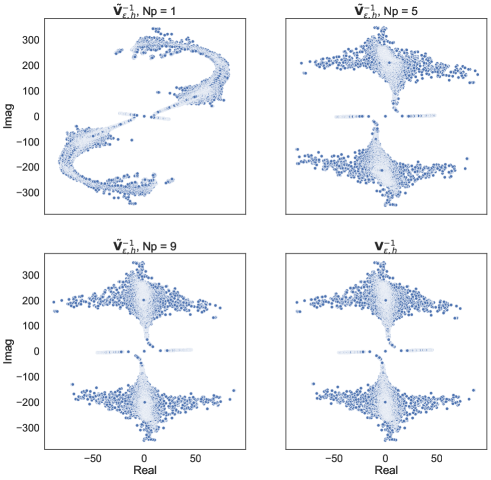
Figure 3: Spectral comparison for $\mathbf{V}_{\varepsilon,h}^{-1}$ and $\tilde{\mathbf{V}}_{\varepsilon,h,N_{p}}^{-1}$. Top left: $N_{p}=1$. Top right: $N_{p}=5$. Bottom left: $N_{p}=9$. Bottom right $\mathbf{V}_{\varepsilon,h}^{-1}$. In all figures, $\kappa=\pi$.

3.5 Implementational simplification

In this section we propose a simplification of the above preconditioner that we believe is novel and reduces its computational effort. In [11] the direct sparse solution of the various systems of the form (21) was proposed. However, depending on the magnitude of the associated Padé coefficients this can be simplified. Consider again the sum

$$\mathbb{I}-\frac{1}{R_{0}}\mathbb{G}\sum_{j=1}^{N_{p}}\frac{A_{j}}{B_{j}}\boldsymbol{\Pi}_{j,\varepsilon,h}^{-1}$$ (24)

contained in (3.4) with

$$\boldsymbol{\Pi}_{j,\varepsilon,h}=\left[\mathbb{G}-B_{j}(\mathbb{N}_{\varepsilon}+\mathbb{L}\mathbb{K}_{\varepsilon}^{-1}(\mathbb{L})^{T})\right].$$

Let $\beta_{j}:=A_{j}/B_{j}$. In Fig. 4 the values of $\beta_{j}$ and $B_{j}$ are shown for varying $j$. We can see heuristically that if $\beta_{j}$ is large, then $B_{j}$ becomes small and when $\beta_{j}$ is small, $B_{j}$ remains bounded. Let us consider those two cases.

If $\beta_{j}$ is small then we can just discard the corresponding term in (24). However, if $\beta_{j}$ is large then $B_{j}$ becomes negligible, and we can apply the simplification:

$$\boldsymbol{\Pi}_{j,\varepsilon,h}=\left[\mathbb{G}-B_{j}(\mathbb{N}_{\varepsilon}+\mathbb{L}\mathbb{K}_{\varepsilon}^{-1}(\mathbb{L})^{T})\right]\approx\mathbb{G}.$$

We hence obtain that

$$\mathbb{I}-\frac{1}{R_{0}}\mathbb{G}\sum_{j=1}^{N_{p}}\frac{A_{j}}{B_{j}}\boldsymbol{\Pi}_{j,\varepsilon,h}^{-1}\approx\left(1-\frac{1}{R_{0}}\sum_{j\in\mathcal{I}}\frac{A_{j}}{B_{j}}\right)\mathbb{I},$$ (25)

where $\mathcal{I}$ is the set of Padé coefficients assumed to be dominant and retained. For all those we perform the approximation $\boldsymbol{\Pi}_{j,\varepsilon,h}\approx\mathbb{G}$. Having this simplification, then (3.4) turns into

$$\vec{\mathbf{r}}_{h}=-K_{\varepsilon,N_{p}}(\mathbb{G}-\mathbb{N}_{\varepsilon})^{-1}\mathbf{S}_{\kappa,h}\vec{\mathbf{r}}_{1,h},$$

where $K_{\varepsilon,N_{p}}$ is a constant. Since we apply the preconditioner on both sides of the equation (as in (3)), we can dismiss the constants and just keep $(\mathbb{G}-\mathbb{N}_{\varepsilon})^{-1}$ as a preconditioner. This is not a direct approximation of the MtE map anymore, but as we will see it still performs well as preconditioner.

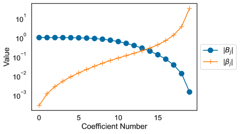
Figure 4: Padé Coefficients $\beta_{j}$ and $B_{j}$ for $N_{p}=50$.

4 Numerical Experiments

This section demonstrates the performance of the proposed OSRC preconditioner and some comparisons with other regularisers. All the tests were performed using Bempp software [20] on a spherical grid of radius $r=1$. In this section we denote by $\tilde{\mathbf{V}}_{\varepsilon,h,A,N_{p}}^{-1}$ the preconditioner obtained by solving the full block systems (21) with a Padé degree $N_{p}$ and by $\tilde{\mathbf{V}}_{\varepsilon,h,B}^{-1}$ the simplified preconditioner $(\mathbb{G}-\mathbb{N}_{\varepsilon})^{-1}$ as described in Section 3.5.

4.1 Validation

The OSRC operator was validated using the same method as in [11], where bistatic RCS are calculated using:

1. Analytic solutions on the unit sphere calculated using spherical harmonics.

2. A direct formulation of the EFIE ($\mathbf{V}_{h}^{-1}$).

3. An approximation of $\mathbf{V}_{\varepsilon,h}^{-1}$, that we calculated by computing the square roots of the eigenvalues of the matrix that generates $\boldsymbol{\Lambda}_{1,\varepsilon}$.

4. By applying $\tilde{\mathbf{V}}_{\varepsilon,h,A,2}^{-1}$.

The first test (Fig. 5) replicates the results obtained in [11] and shows the bistatic RCS obtained from the scattering problem of an incident electromagnetic plane wave by a PEC unit sphere, for $\kappa=\pi$ and $\kappa=8\pi$. The analytic solution and the curve due to $\tilde{\mathbf{V}}_{h}^{-1}$ agree up to plotting accuracy. Moreover, the graphs of $\tilde{\mathbf{V}}_{\varepsilon,h,A,2}^{-1}$ and $\mathbf{V}_{\varepsilon,h}^{-1}$ overlap each other, and both approximate the qualitative behaviour of the bistatic RCS well, though not perfectly.

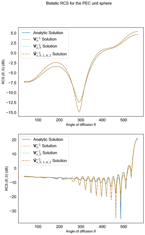
Figure 5: Bistatic RCS for the PEC unit sphere illuminated by an incident electromagnetic plane wave at $\kappa=\pi$ (up) and $\kappa=8\pi$ (down).

4.2 Performance Comparison

In order to compare the performance of the OSRC preconditioner to others, the following attributes were benchmarked:

1. GMRES number of iterations.

2. Assembly and solving times for:

   • Pure direct formulation of the EFIE, denoted by $\mathbf{S}_{\kappa,h}$ (always calculated in the primal grid).

   • EFIE regularised using the Calderón Multiplicative Preconditioner (CMP), denoted by $\mathbf{S}_{\kappa,h}^{2}$.

   • EFIE regularised using the Refinement Free Calderón Multiplicative Preconditioner (RF-CMP), denoted by RF-$\mathbf{S}_{\kappa,h}^{2}$. We must mention that this preconditioner requires the inversion of a dense matrix. The authors in [1] claim that this can be solved by using a multigrid preconditioner that we have not implemented in this work. Having this in mind, the assembly time recorded in this document should be larger than it could be under an optimisation of the method.

     It is necessary to mention that in this case, the Preconditioner is designed to be applied in a discretisation of the EFIE built using RT and NC basis functions as the standard div and curl conforming basis functions. Also, we have solved this system using the conjugate gradient algorithm as suggested by the authors in [1].

   • EFIE regularised with $\tilde{\mathbf{V}}_{\varepsilon,h,A,N_{p}}^{-1}$, with $N_{p}=1,2$.

   • EFIE regularised with $\tilde{\mathbf{V}}_{\varepsilon,h,B}^{-1}$.

These tests were performed using $\mathcal{H}$-matrix compression [13] with an accuracy of around $10^{-3}$ of the compressed matrices.

As expected, in Fig. 6, $\tilde{\mathbf{V}}_{\varepsilon,h,A,N_{p}}^{-1}\mathbf{S}_{\kappa,h}$ shows (slightly) better results than $\tilde{\mathbf{V}}_{\varepsilon,h,B}^{-1}\mathbf{S}_{\kappa,h}$, because the first is a better approximation than the latter. However, in terms of solving time (table3), it could be more convenient to use $\tilde{\mathbf{V}}_{\varepsilon,h,B}^{-1}\mathbf{S}_{\kappa,h}$, since it is considerably cheaper to apply.

Table 2 shows assembly times of the different preconditioners in relationship to the assembly time of the non-preconditioned EFIE. The best result for each column is shown in bold. We note that the $\tilde{\mathbf{V}}_{\varepsilon,h,B}^{-1}$ variant is almost as cheap to assemble as the non-preconditioned system despite still being excellent as preconditioner. We notice our non-optimal implementation of the RF-$\mathbf{S}_{\kappa,h}^{2}$ variant. The CMP $\mathbf{S}_{\kappa,h}^{2}$ suffers in terms of assembly time from the need to assemble operators on the barycentrically refined grid. The solution times in Table 3 also confirm the effectiveness of the OSRC type preconditioners and here in particular the $\tilde{\mathbf{V}}_{\varepsilon,h,B}^{-1}$ variant.

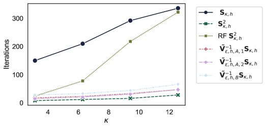
Figure 6: Iterations comparison between different EFIE formulations on a grid with constant relation $\kappa\cdot h$.

Table 2: $\mathbf{T}(\mathbf{R}\mathbf{S}_{\kappa,h})\mathbin{/}\mathbf{T}(\mathbf{S}_{\kappa,h})$ assembly time ratios comparison between different EFIE formulations on a spherical grid with constant relation $\kappa\cdot h$.

Formulation	$\kappa=\pi$	$\kappa=2\pi$	$\kappa=3\pi$	$\kappa=4\pi$
$\mathbf{S}_{\kappa,h}$	1.000	1.000	1.000	1.000
$\mathbf{S}_{\kappa,h}^{2}$	10.043	8.929	13.330	11.173
RF-$\mathbf{S}_{\kappa,h}^{2}$	5.644	23.132	67.077	132.672
$\tilde{\mathbf{V}}_{\varepsilon,h,A,1}^{-1}\mathbf{S}_{\kappa,h}$	1.063	1.141	1.203	1.234
$\tilde{\mathbf{V}}_{\varepsilon,h,A,2}^{-1}\mathbf{S}_{\kappa,h}$	1.129	1.233	1.365	1.434
$\tilde{\mathbf{V}}_{\varepsilon,h,B}^{-1}\mathbf{S}_{\kappa,h}$	1.009	1.014	1.015	1.015

Table 3: $\mathbf{T}(\mathbf{R}\mathbf{S}_{\kappa,h})\mathbin{/}\mathbf{T}(\mathbf{S}_{\kappa,h})$ solving time ratios comparison between different EFIE formulations on a spherical grid with constant relation $\kappa\cdot h$.

Formulation	$\kappa=\pi$	$\kappa=2\pi$	$\kappa=3\pi$	$\kappa=4\pi$
$\mathbf{S}_{\kappa,h}$	1.000	1.000	1.000	1.000
$\mathbf{S}_{\kappa,h}^{2}$	2.168	1.762	1.521	2.279
RF-$\mathbf{S}_{\kappa,h}^{2}$	2.938	17.189	41.086	80.886
$\tilde{\mathbf{V}}_{\varepsilon,h,A,1}^{-1}\mathbf{S}_{\kappa,h}$	0.319	0.293	0.211	0.253
$\tilde{\mathbf{V}}_{\varepsilon,h,A,2}^{-1}\mathbf{S}_{\kappa,h}$	0.575	0.402	0.263	0.351
$\tilde{\mathbf{V}}_{\varepsilon,h,B}^{-1}\mathbf{S}_{\kappa,h}$	0.187	0.309	0.121	0.200

4.3 $\mathbf{V}_{\varepsilon,h}^{-1}$ performance under mesh refinement.

4.3.1 High frequency regime

Figure 7 compares the various preconditioners for fixed wavenumber $\kappa=\pi$ and decreasing mesh width. While the EFIE without preconditioning suffers from the well known ill-conditioning problems all other preconditioners keep the number of iteration bounded or only very slowly increasing.

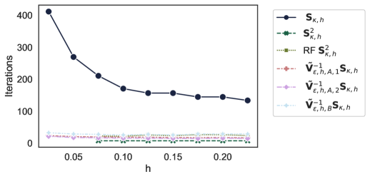
Figure 7: Iterations comparison between different EFIE formulations on a grid with varying discretisation, in the high frequency regime.

4.3.2 Low frequency regime

In this scenario ($\kappa=\pi/10$, Fig. 8), the regularised systems keep showing a robust behaviour. However, the main difference we observe is that the CMP and RF-CMP perform better (in terms of iterations) than the MtE preconditioner. This can be explained by the fact that the latter is based on a high frequency approximation, whereas, the RF-CMP is based on a low frequency approximation.

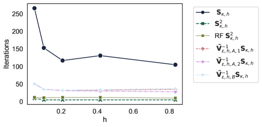
Figure 8: Iterations comparison between different EFIE formulations on a grid with varying discretisation, in the low frequency regime.

4.3.3 Time performance

In terms of time, table 4 shows that in general, assembling $\tilde{\mathbf{V}}_{\varepsilon,h,*,N_{p}}^{-1}\mathbf{S}_{\kappa,h}$ remains cheap as $h\rightarrow 0$. Table 5 shows that the solving time ratios of $\tilde{\mathbf{V}}_{\varepsilon,h,*,N_{p}}^{-1}\mathbf{S}_{\kappa,h}$ improve for smaller $h$ as the number of iterations that takes to solve the problem remains approximately constant. In both regards, assembly and solving time, $\tilde{\mathbf{V}}_{\varepsilon,h,*,N_{p}}^{-1}\mathbf{S}_{\kappa,h}$ outperforms $\mathbf{S}_{\kappa,h}^{2}$ (unless the discretisation is very rough).

Table 4: $\mathbf{T}(\mathbf{R}\mathbf{S}_{\kappa,h})\mathbin{/}\mathbf{T}(\mathbf{S}_{\kappa,h})$ assembly time ratios comparison between different EFIE formulations on a spherical grid with varying discretisation.

$\kappa$	$\pi/10$		$\pi$
Formulation	$h=0.052$	$h=0.833$	$h=0.075$	$h=0.225$
$\mathbf{S}_{\kappa,h}$	1.000	1.000	1.000	1.000
$\mathbf{S}_{\kappa,h}^{2}$	12.589	9.565	11.645	10.450
RF-$\mathbf{S}_{\kappa,h}^{2}$	85.990	2.446	30.652	3.568
$\tilde{\mathbf{V}}_{\varepsilon,h,A,1}^{-1}\mathbf{S}_{\kappa,h}$	1.179	1.104	1.122	1.051
$\tilde{\mathbf{V}}_{\varepsilon,h,A,2}^{-1}\mathbf{S}_{\kappa,h}$	1.221	1.195	1.257	1.077
$\tilde{\mathbf{V}}_{\varepsilon,h,B}^{-1}\mathbf{S}_{\kappa,h}$	1.019	1.049	1.015	1.012

Table 5: $\mathbf{T}(\mathbf{R}\mathbf{S}_{\kappa,h})\mathbin{/}\mathbf{T}(\mathbf{S}_{\kappa,h})$ solving time ratios comparison between different EFIE formulations on a spherical grid with varying discretisation.

$\kappa$	$\pi/10$		$\pi$
Formulation	$h=0.052$	$h=0.833$	$h=0.075$	$h=0.225$
$\mathbf{S}_{\kappa,h}$	1.000	1.000	1.000	1.000
$\mathbf{S}_{\kappa,h}^{2}$	1.629	1.493	1.584	2.489
RF-$\mathbf{S}_{\kappa,h}^{2}$	4.137	0.783	6.040	1.636
$\tilde{\mathbf{V}}_{\varepsilon,h,A,1}^{-1}\mathbf{S}_{\kappa,h}$	0.422	1.104	0.222	0.338
$\tilde{\mathbf{V}}_{\varepsilon,h,A,2}^{-1}\mathbf{S}_{\kappa,h}$	0.552	1.006	0.316	0.457
$\tilde{\mathbf{V}}_{\varepsilon,h,B}^{-1}\mathbf{S}_{\kappa,h}$	0.180	1.430	0.184	0.231

4.4 An example on a less regular surface.

The same tests were performed on a NASA almond-shaped grid, with a wavenumber of $\kappa=2\pi$, to see if the condition number boundedness was preserved on a more interesting shape. Figure 9 shows that, compared to the non-regularised EFIE, the MtE preconditioner allows to solve the problem in considerably less iterations than the non-regularised EFIE, while being substantially cheaper to compute (compared to the CMP preconditioners).

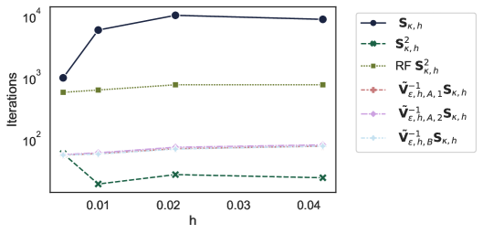
Figure 9: Iterations comparison between different EFIE formulations on an almond-shaped grid with varying $h$.

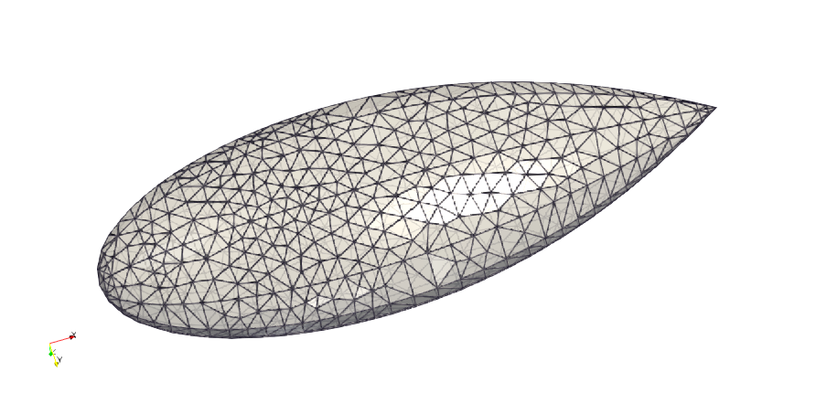
Figure 10: Example of a NASA almond grid.

4.5 Heads up: the MtE on an open surface

Finally, in Fig. 11 we demonstrate the performance of the MtE preconditioner on an open cylinder (see Fig. 12 for the geometry). The formulation is the usual EFIE for screens [9, section 7.1]. As Fig. 11 shows, the iteration count for the MtE preconditioned version behaves very favourably even compared to the CMP adapted to screens.

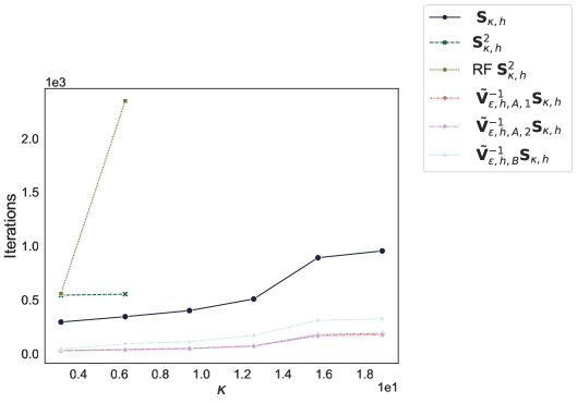
Figure 11: Iterations comparison between different EFIE formulations on an open cylinder grid, with varying $\kappa$.

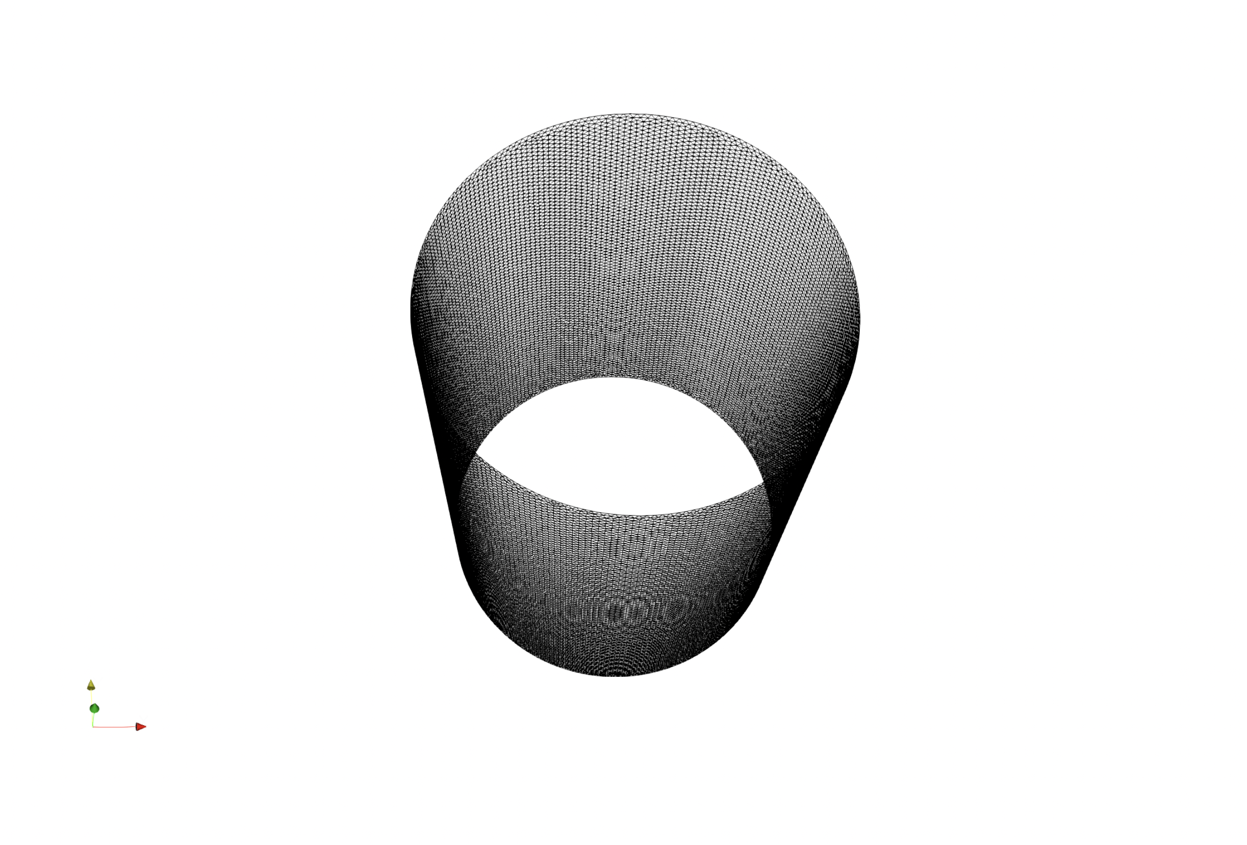
Figure 12: Example of open cylinder grid.

5 Conclusions

The aim of this paper was to test an approximation of the Magnetic to Electric operator proposed in [11] as a preconditioner operator for the EFIE. This operator ($\tilde{\mathbf{V}}_{\varepsilon,N_{p}}^{-1}$) is based on a rational complex Padé approximant of an OSRC ($\mathbf{V}_{\varepsilon}^{-1}$) operator, also proposed in [11].

It was shown that this operator works as a preconditioner for the EFIE and different alternatives for its discretisation were proposed and benchmarked. The results from these tests prove the effectiveness of the proposed preconditioner and that it also outperforms the standard Calderón Multiplicative Preconditioner. It is also competitive with a refinement free version of the CMP, while usually being simpler to implement as it uses just straight forward sparse matrix discretisations of surface differential operators that are often already available or easy to implement within boundary element codes. On top of this, we performed tests on more complex geometries, including an open domain. The results obtained from these tests are very promising, opening the door to the application of this method to more complex open surfaces.

References

- [1] Simon B Adrian, Francesco Paolo Andriulli, and Thomas F Eibert. On a refinement-free Calderón multiplicative preconditioner for the electric field integral equation. Journal of Computational Physics, 376:1232–1252, 2019.
- [2] Francesco P Andriulli, Kristof Cools, Hakan Bagci, Femke Olyslager, Annalisa Buffa, Snorre Christiansen, and Eric Michielssen. A multiplicative Calderón preconditioner for the electric field integral equation. IEEE Transactions on Antennas and Propagation, 56(8):2398–2412, 2008.
- [3] Xavier Antoine and Marion Darbas. Generalized combined field integral equations for the iterative solution of the three-dimensional Helmholtz equation. ESAIM: Mathematical Modelling and Numerical Analysis, 41(1):147–167, 2007.
- [4] Xavier Antoine, Marion Darbas, and Ya Yan Lu. An improved surface radiation condition for high-frequency acoustic scattering problems. Computer Methods in Applied Mechanics and Engineering, 195(33-36):4060–4074, 2006.
- [5] Timo Betcke, Matthew W. Scroggs, and Wojciech Śmigaj. Product algebras for galerkin discretisations of boundary integral operators and their applications. ACM Transactions on Mathematical Software, 46(1):1–22, mar 2020.
- [6] A. Buffa and P. Ciarlet Jr. On traces for functional spaces related to Maxwell’s equations part I: An integration by parts formula in Lipschitz polyhedra. Mathematical Methods in the Applied Sciences, 24(1):9–30, 2001.
- [7] Annalisa Buffa and Snorre Christiansen. A dual finite element complex on the barycentric refinement. Mathematics of Computation, 76(260):1743–1769, 2007.
- [8] Annalisa Buffa, Martin Costabel, and Dongwoo Sheen. On traces for H(curl,) in Lipschitz domains. Journal of Mathematical Analysis and Applications, 276(2):845–867, 2002.
- [9] Annalisa Buffa and Ralf Hiptmair. Galerkin boundary element methods for electromagnetic scattering. In Lecture Notes in Computational Science and Engineering, pages 83–124. Springer Berlin Heidelberg, 2003.
- [10] M. Darbas, E. Darrigrand, and Y. Lafranche. Combining analytic preconditioner and fast multipole method for the 3-d Helmholtz equation. Journal of Computational Physics, 236:289–316, 2013.
- [11] Mohamed El Bouajaji, Xavier Antoine, and Christophe Geuzaine. Approximate local magnetic-to-electric surface operators for time-harmonic Maxwell’s equations. Journal of Computational Physics, 279:241–260, 2014.
- [12] Leslie Greengard and Vladimir Rokhlin. A fast algorithm for particle simulations. Journal of computational physics, 73(2):325–348, 1987.
- [13] Wolfgang Hackbusch. Hierarchical matrices: algorithms and analysis, volume 49. Springer, 2015.
- [14] Andreas Kirsch. The mathematical theory of time-harmonic Maxwell’s equations: expansion, integral, and variational methods. Springer, New York, 2014.
- [15] Gregory Kriegsmann, Allen Taflove, and Koradar Umashankar. A new formulation of electromagnetic wave scattering using an on-surface radiation boundary condition approach. IEEE Transactions on Antennas and Propagation, 35(2):153–161, 1987.
- [16] Fausto A Milinazzo, Cedric A Zala, and Gary H Brooke. Rational square-root approximations for parabolic equation algorithms. The Journal of the Acoustical Society of America, 101(2):760–766, 1997.
- [17] Jean-Claude Nédélec. Acoustic and electromagnetic equations. Springer, New York, 2001.
- [18] Andrey V Osipov and Sergei A Tretyakov. Modern electromagnetic scattering theory with applications. John Wiley & Sons, 2017.
- [19] Sadasiva Rao, Donald Wilton, and Allen Glisson. Electromagnetic scattering by surfaces of arbitrary shape. IEEE Transactions on antennas and propagation, 30(3):409–418, 1982.
- [20] Matthew W Scroggs, Timo Betcke, Erik Burman, Wojciech Śmigaj, and Elwin van’t Wout. Software frameworks for integral equations in electromagnetic scattering based on Calderón identities. Computers & Mathematics with Applications, 74(11):2897–2914, 2017.
- [21] Giuseppe Vecchi. Loop-star decomposition of basis functions in the discretization of the EFIE. IEEE Transactions on Antennas and Propagation, 47(2):339–346, 1999.