Sub-galactic scaling relations with T_e-based metallicity of low metallicity regions in galaxies: metal-poor gas inflow may have important effects?

Abstract

The scaling relationship is a fundamental probe of the evolution of galaxies. Using the integral field spectroscopic data from the Mapping Nearby Galaxies at Apache Point Observatory survey, we select 1698 spaxels with significant detection of the auroral emission line [O iii]$\lambda$4363 from 52 galaxies to investigate the scaling relationships at the low-metallicity end. We find that our sample’s star formation rate is higher and its metallicity is lower in the scaling relationship than the star-forming sequence after removing the contribution of the Fundamental Metallicity Relation.We also find that the stellar ages of our sample are younger ($<$ 1 Gyr) and the stellar metallicities are also lower. Morphological parameters from Deep Learning catalog indicate that our galaxies are more likely to be merger. These results suggest that their low metallicity regions may be related to interaction, the inflow of metal-poor gas may dilute the interstellar medium and form new metal-poor stars in these galaxies during interaction.

1 Introduction

The scaling relationship is important for understanding the formation and evolution of galaxies. One of the well-established relationships is the correlation between the star formation rate (SFR) and the stellar mass (M_∗), which is the so-called star-forming main sequence (SFMS). Another important relationship is the stellar mass–metallicity relation (MZR), which indicates that galaxy metallicities increase with increasing M_∗, and reflects the balance between gravitational potential and galactic feedback. It was established by Lequeux et al. (1979) and has been extended by a series of studies for decades (e.g., Tremonti et al., 2004; Mannucci et al., 2010).

The SFMS and MZR are both established primarily by global galactic parameters. It is also important to understand whether galactic local parameters (e.g., stellar mass surface density ($\Sigma_{*}$), SFR surface density ($\Sigma_{\rm SFR}$), and local metallicity) are more fundamental to probe the global SFMS and MZR. Recently, with the emergence of integral field spectroscopy (IFS) surveys, spatially resolved scaling relationships have also been developed. Rosales-Ortega et al. (2012) demonstrated the existence of a local relation between $\Sigma_{*}$, metallicity, and $\Sigma_{\rm SFR}$ using 38 nearby galaxies from the PPAK IFS Nearby Galaxies Survey (Rosales-Ortega et al., 2010) and the Calar Alto Legacy Integral Field spectroscopy Area (CALIFA; Sánchez et al., 2012) survey. Cano-Díaz et al. (2016) found a spatially resolved SFMS on $\sim$1 kpc scale with a slope of $\sim$0.7 in the local universe from CALIFA IFS data. More further researches on the spatially resolved scaling relationship also followed on (e.g. Barrera-Ballesteros et al. 2016; Gao et al. 2018, hereafter G18; Liu et al. 2018).

The metal-poor galaxies/regions play an essential role in galaxy evolution, especially for the galaxies at the early stage of evolution, or for those that evolve slowly. Understanding the various properties of galaxies at low metallicity in the MZR can help us uncover some important processes in galaxy evolution. Low metallicities of galaxies/regions suggest that they might have significant metal-poor gas inflows or metal-enriched gas outflows. (Kunth & Östlin, 2000). However, the slope and scatter of the low metallicity end of the local MZR is still not clear currently. The reason is that current methods of investigating the local MZR are mainly based on the strong emission lines method, which may be not accurate enough for the calibration of low metallicity (López-Sánchez et al., 2011). The electron temperature ($T_{\rm e}$) method (Aller, 1984; Izotov et al., 2006; Pilyugin et al., 2010), which is also called direct method, base on the anticorrelation between metallicity and $T_{\rm e}$, can obtain the metallicity directly and avoid the systematic error of low metallicity with high ionization parameter. It needs auroral line ratios such as [O iii]$\lambda$4363/[O iii]$\lambda\lambda$4959,5007 to calculate $T_{\rm e}$. Auroral lines are two order of magnitude fainter than strong lines, which makes the direct method very challenging to apply. But with the sample size of the current IFS surveys rapidly expanding recent years, we finally have the dataset to apply direct method by searching for resolved [O iii]$\lambda$4363 emission lines for a large and representative sample of galaxies.

In this work, we select H ii regions with significant [O iii]$\lambda$4363 emission line dectection from SDSS-IV Mapping Nearby Galaxies at Apache (MaNGA) survey (Bundy et al., 2015) and present their local SFMS and MZR. The paper is organized as follows. Section 2 describes the sample selection and the calculation of physical parameters. Section 3 presents our main results. Section 4 discusses influences of metallicity calibrations and the potential role of merges in our sample. Finally, Section 5 comes up with our conclusions. We adopt a flat cosmology with $\Omega_{\Lambda}$ = 0.7, $\Omega_{M}$ = 0.3 and $H_{0}$ = 70 km s^-1 Mpc^-1 to determine distance-dependent measurements.

2 Data

2.1 MaNGA DR15 Overview

The MaNGA survey, one of the three core programs in the SDSS-IV (Blanton et al., 2017), is an IFS survey targeted at $\sim 10,000$ nearby galaxies that are selected from the NASA-Sloan-Atlas catalog (NSA; Blanton et al., 2011; Bundy et al., 2015). The redshifts of these target galaxies span a range of $0.01<z<0.15$. The spectral coverage is 3600–10300 Å with a resolution of R $\sim$ 2000 (Drory et al., 2015). The full width at half maximum (FWHM) of the reconstructed point-spread function is about 2$\farcs$5 (Law et al., 2016). Recently, the SDSS DR15 publicly released IFS observations and ancillary data products of 4621 galaxies (Aguado et al., 2019). Comparing with DR14, there are many improvements in DR15, with Data Reduction Pipeline (DRP; Law et al., 2016), such as the flux calibration and spetral line-spread function estimation. DR15 also provides an entirely new Data Analysis Pipeline products (DAP; Westfall et al., 2019), which provides the measurements of Balmer series lines and strong forbidden lines, including [O ii]$\lambda$3727, [O iii]$\lambda\lambda$4959,5007, and [N ii]$\lambda$6583 (Belfiore et al., 2019), facilitating our data analysis. In this work, we treat these 4621 galaxies from DRP and DAP as the parent sample.

2.2 Rough Sample Selection

In order to identify regions with strong [O iii]$\lambda$4363 from all MaNGA data cubes more efficiently , we first select spaxels according to the following criteria:

1. $b/a\geqslant 0.3$,

2. no “bad” flag in “DRP3QUAL”,

3. S/N(H$\alpha$) $\geqslant$ 3, S/N(H$\beta$) $\geqslant$ 3, S/N([O iii]$\lambda$3727) $\geqslant$ 3, S/N([O iii]$\lambda\lambda$4959,5007) $\geqslant$ 3, S/N([N ii]$\lambda$6583) $\geqslant$ 3, and S/N([O iii]$\lambda$4363) $\geqslant$ 5,

4. not active galactic nuclei (AGN).

The values of $b$/$a$ are from the NSA catalog, representing the projected ratio of the semi-minor axis to the semi-major axis of galaxies. This limitation is to avoid the severe dust attenuation in galactic disks. The fluxes and noises of all emission lines except [O iii]$\lambda$4363 are derived based on the DAP hybrid bin, while the fluxes and noises of [O iii]$\lambda$4363 are fitted to a single Gaussian profile by ourselves following Ly et al. (2014). All data of emission lines have been processed by Galactic extinction correction, moving to rest frame, and intrinsic dust extinction correction in turn. We use the color excess $E(B-V)$ map of the Milky Way (Schlegel et al., 1998) and the Cardelli et al. (1989) extinction law to correct Galactic extinction and use the Balmer decrements under the Case B recombination and apply the Calzetti et al. (2000) attenuation law to correct intrinsic dust extinction. For spaxels with H$\alpha$/H$\beta<$2.86 (Hummer & Storey, 1987), we assume the extinction as zero. The [N ii]-based BPT diagnostic diagram (Baldwin et al., 1981) is adopted to avoid possible AGN contamination, and only spaxels below the Kauffmann et al. (2003a) demarcation curve are selected. Thus, we obtain a rough selected sample with 3565 spaxels.

2.3 Spectral Fitting and Further Sample Selection

In Section 2.2, to search for spaxels with obvious [O iii]$\lambda$4363 emission line quickly, we fit the spectra with single Gaussian profile without subtracting stellar continuum. So the selection is rough and is needed to be refined. In this Section, we refit the stellar continuum and emission lines for our rough selected sample.

Following the procedure of Gao et al. (2017), we use the STARLIGHT software (Cid Fernandes et al., 2005) to obtain the best-fit stellar continua, which are then subtracted from the observed spectra. The fitting is based on the built-in stellar library (Bruzual & Charlot, 2003) of STARLIGHT and a Chabrier (2003) initial mass function (IMF). The stellar library includes 45 single stellar populations, consisting of 15 stellar ages ($t_{*}$, ranging from 1 Myr to 13 Gyr) and 3 different stellar metallicities ($Z_{*}$ = 0.004, 0.02, and 0.05). Several stellar properties, such as M_∗, $Z_{*}$, and $t_{*}$, can be derived from the output of STARLIGHT. In order to ensure the consistency of flux measurements, we use the MPFIT (Markwardt, 2009) to refit emissions lines that we are interested in (e.g., [O ii]$\lambda$3727, [O iii]$\lambda$4363, H$\beta$, [O iii]$\lambda\lambda$4959,5007, H$\alpha$, [N ii]$\lambda\lambda$6548,6583, [S ii]$\lambda\lambda$6717,6731). After obtaining the fluxes of emission lines, we apply Balmer decrement (Hummer & Storey, 1987) and Calzetti et al. (2000) attenuation curve to them again. Finally, we get the final emission fluxes of this work, rather than the DAP data and the rough flux measurements in Section 2.2. In order to verify the accuracy of our fitting, we compared our fitting results with the DAP results. Details of the comparison are in Appendix A.

Because [O iii]$\lambda$4363 emission might be contaminated by cosmic rays or other noise, further selection is needed to remove fake detection. First of all, we remove galaxies whose spaxel numbers in the rough selected sample are less than 5. Then, we calculate the S/N ratio at $\lambda$ = 4020 Å and remove the spaxels with S/N$<$5 to ensure that the uncertainty of stellar mass are less than 0.11 dex (Cid Fernandes et al., 2005). Spaxels whose fluxes of [O iii]$\lambda$4363 are too excessive to calculate an vaild metallicity are also removed, which may be caused by noise. Next, we manually check the continuum fitting status and emission line fitting status of each spectrum. We remove those spectra whose [O iii]$\lambda$4363 lines do not have well-defined profiles or velocities have significant deviation from other emission lines. After manual inspection, our final sample consists of 1698 spaxels from 52 different galaxies.

In addition, we also select all star-forming regions in these 52 galaxies. The requirements of S/N are the same as those of the [O iii]$\lambda$4363 regions without the [O iii]$\lambda$4363 emission line to calculate their metallicities applying the strong line method.

2.4 SFR Surface Density and Metallicity Calculation

2.4.1 SFR Surface Density

We use the H$\alpha$ luminosity to determine the dust-corrected SFR for each spaxel, assuming a Chabrier (2003) IMF. The SFR calibration from Kennicutt (1998) is:

$${\rm SFR(M_{\odot}~{}yr^{-1})}=4.4\times 10^{-42}L_{\mathrm{H}\alpha}\mathrm{(erg~{}s^{-1})}.$$ (1)

The size of each spaxel of MaNGA is $0\farcs 5\times 0\farcs 5$, so the projection corrected area is given by

$$A=\left[D(z)\times 0.5\times\frac{\pi}{3600\times 180}\right]^{2}\times\frac{1}{b/a},$$ (2)

where $D(z)$ is the angular diameter distance of the galaxy. As a result, the $\Sigma_{\rm SFR}$ and $\Sigma_{*}$ of each spaxel are

$${\rm\Sigma_{SFR}=SFR/}A,$$ (3)

$$\Sigma_{*}=M_{*}/A.$$ (4)

2.4.2 $T_{\rm e}$ and Oxygen abundence

Here, we adopt the formulation from Pilyugin et al. (2010) to calculate the $T_{\rm e}$, O²⁺ abundance and O⁺ abundance of each spaxel. For our metallicity estimation, we adopt a standard two-zone temperature model with $t_{2}$ = 0.672 $t_{3}$ + 0.314 (Pilyugin et al., 2009). Because the most important ions of oxygen in H ii regions are O⁺ and O²⁺, we take the sum of the abundance of these two ions as the abundance of oxygen.

To all star-forming spaxels without the requirement of S/N([O iii]$\lambda$4363)$\geqslant$3 which are described at the end of Section 2.3, we apply the R calibration relation from Pilyugin & Grebel (2016)(hereafter PG16), which is calibrated from the T_e metallicities of 313 H ii regions, ranging from 12+log(O/H)$\sim$7.0 to $\sim$8.7. with a mean difference of 0.049 dex.

2.5 Uncertainty Estimate

Our uncertainty consists of two parts, part one is converted from the error spectrum provided by MaNGA DATACUBE ($\sigma_{\rm errspec}$) , and part two comes from 2 independent observations of the same galaxy (8256-9102 and 8274-9102) in our sample ($\sigma_{\rm indepobs}$). Our final uncertainty $\sigma$ is determined by rooting the sum of the squares of the above two parts:

$$\sigma=\sqrt{\sigma_{\rm errspec}^{2}+\sigma_{\rm indepobs}^{2}}.$$ (5)

For uncertainties of $\Sigma_{\rm SFR}$ and 12+log(O/H) from the error spectrum ($\sigma_{\rm errspec}$), we adopt a Monte-Carlo method and repeat the calculation for 1000 times. For every spectrum, we produce a series of fluxes for each emission line with a Gaussian distribution, assuming its average as the measured line flux and standard deviation as the measured error. The median of metallicity uncertainty is 0.07 dex, and the median of $\Sigma_{\rm SFR}$ uncertainty is 0.008 dex. For uncertainties of $\Sigma_{*}$ from the error spectrum, we directly adopt 0.11 dex (Cid Fernandes et al., 2005), because the S/N ratios of our continuua are all grater than 5.

For uncertainties from 2 independent observations, we can get a distribution by taking the difference of the quantities at the same coordinates. We use the standard deviation of this distribution as the uncertainty. The standard deviations ($\sigma_{\rm indepobs}$) of $\Sigma_{\rm SFR}$, $\Sigma_{*}$ and metallicity are 0.10 dex, 0.17 dex and 0.10 dex, respectively. The final uncertainty ($\sigma$) of $\Sigma_{\rm SFR}$, $\Sigma_{*}$ and metallicity are 0.10 dex, 0.20 dex and 0.12 dex, respectively.

3 Result

Comparing to previous studies (e.g., Barrera-Ballesteros et al., 2016; Gao et al., 2018), this work uses the newest DR15 data as the initial sample and focuses on the [O iii]$\lambda$4363 selected star-forming regions. Because of the weakness of [O iii]$\lambda$4363 emission lines, our sample is much smaller than normal star forming sample, and its overall properties are also much different form those of normal star forming sample. The SDSS images and metallicity profiles of 4 galaxies with the most spaxels in our 52 [O iii]$\lambda$4363 selected sample are shown in Figure 1. Other galaxies are shown in Appendix B. We perform a linear fit to the profile of the metallicity of each galaxy along the radius.

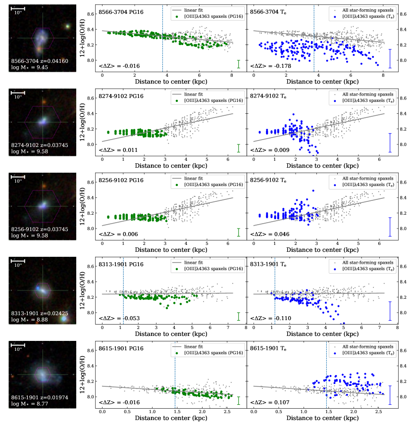
Figure 1: Left panel: the SDSS images of 5 galaxies with the most spaxels in our 52 [O iii]$\lambda$4363 selected sample. The field of view of each image is 50″. Right panel: the radial profiles of the metallicity of the corresponding galaxy. Gray dots are all star-forming spaxels without the requirement of S/N([O iii]$\lambda$4363)$\geqslant$3, which are described at the end of Section 2.3. Gray lines are the linear fit of gray dots. Green dots and blue dots represent the PG16 and T_e calibrated metallicity of our [O iii]$\lambda$4363 selected spaxels, respectively. The vertical dashed line represents the effective radius of the galaxy. Both 2 independent observations of the same galaxy (8274-9102 and 8256-9102) are shown in the second and third row of the figure, respectively.

3.1 Global SFMS and Morphology

Table 1: Basic information of 30 galaxies with the most spaxels in our sample

Galaxy ID	Count	RA	DEC	Redshift	M∗	M∗	SFR	T-Type	P(merge)
[plate]-[ifu]		(deg)	(deg)		(log(M∗/M⊙))	(log(M∗/M⊙))	(log(M⊙/yr))
8566-3704	173	115.22481	40.06964	0.04160	9.45	$-$	$-$	4.30	0.99
8274-9102*	124	165.10414	43.01969	0.03745	9.58	9.02	0.52	7.00	0.34
8313-1901	84	240.28713	41.88075	0.02425	8.88	9.28	-0.04	1.90	0.18
8615-1901	79	321.07220	1.02836	0.01974	8.77	8.95	-0.06	4.55	0.38
9000-6102	68	170.88396	53.46820	0.02719	9.45	9.41	-0.05	5.27	0.73
7495-6102	62	204.51286	26.33821	0.02615	8.74	8.96	0.12	5.80	0.06
8942-3703	60	124.38507	28.35783	0.01986	8.67	8.85	-0.21	4.43	0.04
8551-1902	54	234.59171	45.80194	0.02135	8.43	8.90	-0.13	1.74	0.04
8465-6102	48	197.54970	48.62339	0.02828	9.29	8.93	0.40	3.08	0.96
8548-9102	48	244.91463	47.87321	0.02094	8.70	8.87	-0.22	5.99	0.79
8455-9101	47	157.18363	39.77859	0.03004	9.66	9.53	0.13	5.46	0.79
8322-9101	44	199.60756	31.46795	0.01869	9.54	$-$	$-$	5.31	0.89
8548-3702	43	243.32681	48.39181	0.01990	8.74	8.87	-0.44	4.47	0.45
8257-3704	43	165.55361	45.30387	0.02022	8.69	9.00	-0.65	10.00	0.04
8719-12702	41	120.19928	46.69053	0.01938	9.49	9.65	-0.04	5.57	0.43
8727-3702	41	54.55405	-5.54040	0.02215	8.48	8.76	-0.16	-1.16	0.04
8239-12704	40	117.45125	48.12956	0.01808	9.42	9.29	-0.39	6.09	0.31
8241-6101	40	127.04853	17.37466	0.02087	8.63	8.62	-0.38	5.98	1.00
8996-12703	37	171.97836	53.00109	0.02134	8.84	8.13	-0.29	6.59	0.78
8715-12704	37	121.17245	50.71853	0.02262	8.77	8.96	-0.12	6.16	0.11
8987-6103	33	137.26802	28.25683	0.02166	8.67	8.64	-1.93	5.12	0.30
8936-6104	32	117.92943	30.44875	0.01424	8.65	6.99	-1.90	4.64	0.09
8987-9101	28	137.44943	27.86231	0.02044	8.94	8.94	-0.69	4.90	0.02
8552-6101	28	227.01700	42.81902	0.01801	8.66	8.64	-0.88	5.74	0.82
9509-3702	27	122.43975	25.88031	0.02511	9.27	9.70	0.45	4.65	1.00
8147-9102	27	118.85282	26.98635	0.01524	8.85	8.83	-0.98	5.28	0.38
8553-12703	25	235.95318	57.23323	0.01355	8.61	6.20	-2.10	5.65	0.34
8325-12702	24	209.89514	47.14768	0.04204	9.28	9.50	0.43	6.35	0.17
8458-3702	23	147.56250	45.95731	0.02487	9.44	7.34	-0.29	3.94	0.68
8083-12705	22	50.17898	-1.10865	0.02091	10.09	10.02	-0.03	5.44	0.34

Note. — From left to right, the columns correspond to (1) galaxy ID, defined as the [plate]-[ifudesign] of the MaNGA observations; (2) the count of [O iii]$\lambda$4363 spaxels; (3) and (4) the ra and dec of IFU; (5) the redshift taken from NSA catalog; (6) the total M_∗ taken from NSA sersic mass; (7) the total M_∗ taken from MPA-JHU catalog, some of galaxies (3 in 52) can not match the catalog, which have a empty value; (8) SFR taken from MPA-JHU catalog, some of galaxies can not match the catalog, which have a empty value; (9) the T-Type value of morphology derived from DL catalog (T-Type ¡ 0 for ETGs, T-Type ¿ 0 for LTGs, T-Type $\sim$ 0 for S0), whose methodology for training and testing the DL algorithm is described in Domínguez Sánchez et al. (2018); (10) the probability of merger signature (or projected pair) derived from the DL catalog same as (9).

Note. — *: MaNGA has two independent observations (8256-9102 and 8274-9102) of this galaxy, here we only select the observation (8274-9102) with less uncertainty of metallicity.

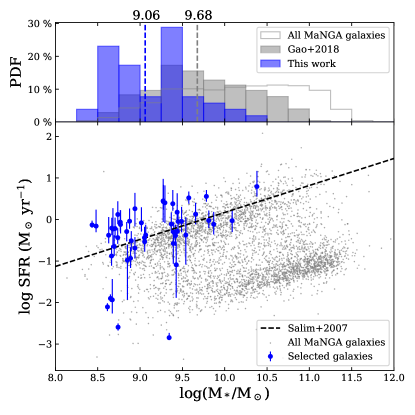
Figure 2: Top panel: the histograms of normalized M_∗ distribution. The blue filled histograms represent our 52 [O iii]$\lambda$4363 emission galaxies, the gray filled histograms represent star forming sample in G18, and the gray hollow histograms all MaNGA galaxies in DRP catalog. The vertical dashed lines of different colors respectively indicate the median of the corresponding mass distribution. Bottom panel: M${}_{*}-$ SFR relation (SFMS) of MaNGA galaxies. Blue dots represent our 50 sample galaxies (4 of 52 galaxies can not be matched in MPA-JHU catalog), whose error bars represent 1$\sigma$ error (16% $\sim$ 84%). Gray dots are all of the galaxies in MaNGA DR15 data. The main-sequence relation for SFGs in the local universe (Salim et al., 2007) is shown as the black dashed line.

We first investigate the global properties of these galaxies. Figure 2 shows the mass distribution and the M${}_{*}-$SFR relation (global SFMS) comparing with all MaNGA galaxies and SFGs in G18 which contains 1122 galaxies and 8 $\times$ 10⁵ spaxels. SFRs are retrieved from the MPA-JHU catalog (Kauffmann et al., 2003b). Galaxies whose SFR are not available in the MPA-JHU catalog are not shown in the figure. We can see that our [O iii]$\lambda$4363 selected galaxies are located in the upper star forming region, and their total M_∗ are lower than the rest of the normal SFGs. The median mass (log (M_∗/M_⊙)) of our [O iii]$\lambda$4363 selected galaxies is 9.25 and the median mass (log (M_∗/M_⊙)) of SFGs in G18 is 9.68. However, we have noticed that some of our sample are located too low on the M${}_{*}-$SFR diagram, indicating that these galaxies may not be star-forming. We have checked these galaxies and find that there are indeed local star-forming regions in these low-SFR galaxies. This indicates that a galaxy with a lower global SFR may also has more intense star formation locally.

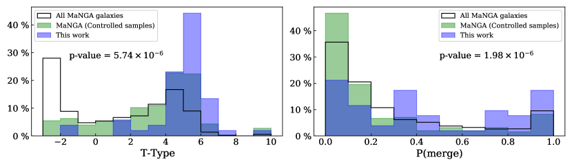
Figure 3: The normalized morphology properties distribution. Morphology data are from the MaNGA Deep Learning DR15 Morphology catalog (DL; Domínguez Sánchez et al., 2018). Blue filled histograms are the final [O iii]$\lambda$4363 sample in this work. Black hollow histograms are the distribution of all galaxies in the DL catalog. Green filled histograms are the controlled sample of galaxies whose M_∗ and SFR distributions are similar to the distribution of our final sample. Each vertical axis is the percentage of the total sample occupied by each bin. The $p$-values of Kolmogorov-Smirnov test between our final sample and controlled sample is also shown in each panel.

Subsequently, we match the MaNGA Deep Learning DR15 Morphology catalog (DL; Domínguez Sánchez et al., 2018) to extract their morphological parameters, the T-Type value and the probability of merger, which have been widely used in previous works (e.g., Meert et al., 2014; Fischer et al., 2018; Chen et al., 2020). This catalog is trained by Deep Learning algorithms using Convolutional Neural Networks based on the catalog of Nair & Abraham (2010) and color images. Due to the particularity of our sample in M_∗ and SFR, which may cause a systematic offset in morphological parameters, we select galaxies with the same M_∗ and SFR distributions as our sample from the MaNGA survey to construct a controlled sample. The distributions of morphology are shown in Figure 3. Here we regard galaxies with a merger probability greater than 0.7 as merger. We found that 18 galaxies in our 52 sample galaxies are merging, accounting for 34.6%, which is higher than the 14.8% of all MaNGA galaxies and 13.0% of controlled sample. We also perform a Kolmogorov-Smirnov test between our sample and the controlled sample and get the $p$-value of T-Type $\sim$ 10^-6, and the $p$-value of P(merge) $\sim$ 10^-10. Table 1 show the picture and information of the 30 galaxies with the most spaxels in our final, which occupy the main part ($\sim$84%) of our all spaxels. From their pictures, we can see that they are all blue in color and irregular in morphology, and some of them seem to be interaction. These observational features are consistent with the morphological parameters from the DL catalog. More details will be discussed in Section 4.3. Therefore, we can conclude that the galaxies we selected not only have lower M_∗ and higher SFR, but also later type and higher merger ratio in morphology, and this is not because of their low M_∗ and high SFR.

We also check the locations of our selected spaxels in these sample galaxies. We find that most spaxels are located within a single star forming region. Regions of most galaxies (42 galaxies) are located in the periphery of the galaxy. Regions of 8 galaxies are in the center of the galaxy. 2 are distributed in the entire galaxy, and the remaining two can not be distinguished because their host galaxies have lower projected axis ratio.

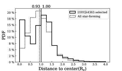
Figure 4: The normalized distribution of the distance to the center of galaxy. Distance is relative to R_e, corrected by projection. Solid border histograms represent the sample we selected by [O iii]$\lambda$4363. Dashed border histograms represent all star-forming spaxels in our sample galaxies. The vertical lines respectively indicate the median of the corresponding border style.

Here we compare the location distribution of our [O iii]$\lambda$4363 selected spaxels in our 52 galaxies and the star-forming spaxels in the same galaxy (Figure 4). The distances to the center are in units of effective radius(R_e) and have already been corrected by $b/a$. It is found that there is no obvious deviation between the location distribution of our regions and the overall star-forming regions.

3.2 Local Properties and Scaling Relations

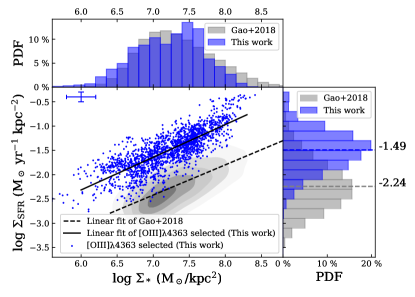
Figure 5: Local SFMS: blue represents our [O iii]$\lambda$4363 selected spaxels, and gray represents star forming spaxels from G18. Histogram: the normalized distribution of the values corresponding to the coordinate axis. The dotted line indicates the median of the distribution of the corresponding color. Scatter diagram: the local main-sequence relation and bottom panel is the $\Sigma_{*}-Z$ relation. Blue dots are our sample, and the gray contour lines represent the distribution of 85% of normal star forming spaxels in G18, and each contour encloses 15%. Black solid lines are the linear fit of our sample. The dashed line is the linear fit of G18’s local SFMS. The error bars of x and y axis are the uncertainty of $\Sigma_{*}$ and $\Sigma_{\rm SFR}$ described in Section 2.5 with an error of $\sim$0.20 dex and $\sim$0.10 dex, respectively.

Since MaNGA has spatially resolved IFU spectra, the main focus of this work is on the local properties of these galaxies, such as $\Sigma_{*}$, $\Sigma_{\rm SFR}$, local metallicity and their scaling relationship. The $\Sigma_{*}-\Sigma_{\rm SFR}$ relationship is plotted in Figure 5, and $\Sigma_{*}-Z$ is plotted in Figure 6. The edges of the diagram show the normalized distributions of the corresponding parameters. The scatter panel shows the local SFMS: $\Sigma_{*}-\Sigma_{\rm SFR}$ relation for our [O iii]$\lambda$4363 selected spaxels. We perform a linear fit to our spaxels and find that

$${\log\rm\Sigma_{SFR}=(0.67\pm 0.01)\log\Sigma_{*}-(6.35\pm 0.09)}.$$ (6)

The correlation coefficient is 0.80, and the residual standard deviation is 0.24. The uncertainties of slope and intercept are obtained by 1000-times bootstrap method, and following fittings are also the same. The units of $\Sigma_{*}$ and $\Sigma_{\rm SFR}$ are M_⊙ kpc^-2 and M_⊙ yr^-1 kpc^-2 respectively. Similar fit is done for the star forming spaxels in G18 and results in

$${\log\rm\Sigma_{SFR}=(0.61\pm 0.00)\log\Sigma_{*}-(6.71\pm 0.03)}.$$ (7)

The correlation coefficient is 0.61, and the residual standard deviation is 0.39. We can see that our sample have higher $\Sigma_{\rm SFR}$ than G18’s sample at a given $\Sigma_{*}$. There is also a significant gap in the median of log $\Sigma_{\rm SFR}$. Ours is -1.49 while G18’s is -2.24. Only 10 spaxels (0.56%) of our sample are within 1$\sigma$ (68%) dispersion of the local SFMS of G18. These results indicate that the SFR of our sample is higher than that of the star formation sequence.

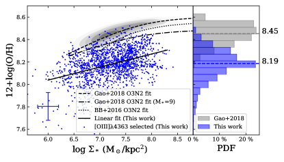
Figure 6: Local MZR: legends are the same as Figure 5 but the dashed curve is the fit of G18’s $\Sigma_{*}-Z$ relation, and the dotted dashed curve is the fit of G18’s M${}_{*}-\Sigma_{*}-Z$ relation when M_∗=9. The dotted curve is from Barrera-Ballesteros et al. (2016). The error bars of x and y axis are the uncertainty of $\Sigma_{*}$ and metallicity described in Section 2.5 with an error of $\sim$0.20 dex and $\sim$0.12 dex, respectively.

Figure 6 shows the local MZR ($\Sigma_{*}-Z$ relation) of our sample and normal star forming sample based on O3N2 method in G18. We note that the O3N2 calibration adopted by G18 is the ONS-based one from (Marino et al., 2013, here after M13). This may cause a systematic deviation from the $T_{\rm e}$ method. We thus transform all metallicities data in G18 into the $T_{\rm e}$-based calibration by the following equation:

$$\begin{split}\rm 12+log(O/H)_{O3N2,T_{e}}=8.533\\ \rm-\frac{8.505-12+log(O/H)_{O3N2,ONS}}{0.221}\times 0.214\end{split}$$ (8)

For our sample, it is also found that the metallicity increases with increasing $\Sigma_{*}$, but the dispersion is large. We find that 221 spaxels (13.0%) of our sample are within 1$\sigma$ dispersion of the local MZR of G18. We simply perform a linear fit to our spaxels and find that

$${\rm 12+\log{(O/H)}=(0.12\pm 0.01)\log\Sigma_{*}+(7.34\pm 0.05)},$$ (9)

with a correlation coefficient of 0.41, and a residual standard deviation of 0.13.

We plot the best fit $\Sigma_{*}-Z$ relation of G18’s radial bin sample. Taking into account the weak influence of the total M_∗ on the local metallicity (Barrera-Ballesteros et al., 2016; Gao et al., 2018) and the smaller M_∗ of our galaxies (see Section 3.1), the best-fit M${}_{*}-\Sigma_{*}-Z$ relation at M${}_{*}=10^{9}$ M_⊙ is also given to eliminate the influence of the total stallar mass of galaxies.

In Figure 6, we can see that the $\Sigma_{*}-Z$ relation of our [O iii]$\lambda$4363 selected spaxels is still systematically lower than that of the normal star forming spaxels in MaNGA when considering the total M_∗. These spaxels with high $\Sigma_{*}$ have anomalously low metallicity (ALM), which are similar to the ALM regions mentioned in Hwang et al. (2019). More details will be discussed in Section 4.3.

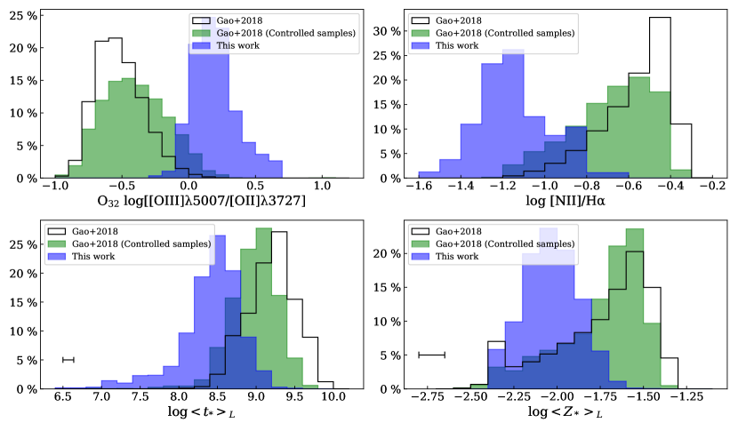
Figure 7: Normalized local properties distribution. Blue filled histograms are the final [O iii]$\lambda$4363 spaxels in this work. Black hollow histograms are the distribution of all star forming spaxels in G18. Green filled histograms are the controlled sample of spaxels in G18 whose $\Sigma_{*}$ and $\Sigma_{\rm SFR}$ distribution are similar to the distribution of our sample. Each vertical axis is the percentage of the total sample occupied by each bin. Top 2 histograms: distributions of O₃₂ and N2 diagnostics. Bottom 2 histograms: distributions of light-weighted stellar properties. The unit of $t_{*}$ is year, and $Z_{*}=Z/Z_{\odot}$. The error bars are uncertainties from STARLIGHT when the signal-to-noise ratio of continuum is 5.

We next investigate and compare the local ionized gas properties and stellar properties through emission lines and continuum of spaxels.

The upper two panels of in Figure 7 show distributions of two emission line ratios O₃₂=log([O iii]($\lambda$4959+$\lambda$5007)/[O ii]$\lambda$3727) and N2=log([N ii]$\lambda$6583/H$\alpha$), while the lower ones are the distributions of the luminosity-weighted $t_{*}$ and $Z_{*}$ obtained by STARLIGHT fitting. Among them, O₃₂ can roughly characterize ionization parameters (Kewley et al., 2019), and N2 can roughly characterize their metallicities (Pettini & Pagel, 2004). The unit of $t_{*}$ is year, and stellar metallicity $Z_{*}=Z/Z_{\odot}$. When the S/N of continuum is 5, the uncertainties of log$\langle t_{*}\rangle_{L}$ and log$\langle Z_{*}\rangle_{L}$ are 0.14 dex and 0.15 dex respectively (Cid Fernandes et al., 2005), which are displayed by error bars.

Since the SFR of our sample is relatively high overall, and we have noticed the possible local Fundamental Metallicity Relation (FMR; Mannucci et al., 2010) which means that regions with higher SFRs tend to have lower metallicities at fixed $\Sigma_{*}$. In order to verify whether our low metallicities are the result of high $\Sigma_{\rm SFR}$ through FMR, here we also need to control the sample likes Section 3.1. Green histograms in Figure 7 show the distributions of the corresponding properties for the sub-sample randomly selected from G18, containing 2499 spaxels, whose distribution on the $\rm\Sigma_{*}-\Sigma_{SFR}$ plane is the same as that of our final [O iii]$\lambda$4363 sample. Thus we can eliminate the potential impact of FMR.

The distribution of data shows that the ionization parameters, gas phase metallicity, $t_{*}$ and $Z_{*}$ of our sample are obviously different from those of all sample and the controlled sample in G18. There is only a small difference between the controlled sample and all sample. Therefore, we can conclude that the spaxels we selected not only have higher $\rm\Sigma_{SFR}$, but also higher ionization parameter, lower gas phase and stellar metallicity and younger stars, and this is not because of their high $\rm\Sigma_{SFR}$ under the impact of FMR.

3.3 Nitrogen abundances

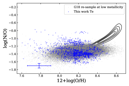
Figure 8: The 12+log(O/H) $-$ log(N/O) relation. The blue dots represent the T${}_{\rm e}-$based result of this work. The black solid contours trace the number density distribution of G18 spaxels, whose O and N abundances are both derived from PG16, and the gray dots correspond to re-sampling 12+log(O/H) $<$ 8.3 data points of G18 by randomly adding Gaussian noise with the same standard deviation as blue dots. The error bar in the lower left corner represents the typical uncertainty of our sample on the two axes.

Metals are direct products of stellar nucleosynthesis, elements originate from different nucleosynthetic can probe the star formation history and chemical enrichment in galaxies. Here we calculate the abundance rations between nitrogen (mostly produced via primary nucleosynthesis in low metallicity regions, as well as secondary nucleosynthesis of low-mass and intermediate-mass stars from higher metallicity regions) and oxygen (mostly produced by massive stars on short time-scales). The N/O probes the star formation time scale, and N/O $-$ O/H diagram can also provides a test of the validity of our Te-based abundances.The calculation method used is also from Pilyugin et al. (2010). Since the [N ii]$\lambda$5755 line is too weak to be detected, we use t₂ estimated from t₃ instead of t_2,N to derive the nitrogen abundance. The 12+log(O/H) $-$ log(N/O) relation is shown in Figure 8. The uncertainty of log(N/O) is $\sim$0.06 dex, which is obtained using the same process as Section 2.5. From Figure 8 we can find that our samples are distributed at the flat low end of the relationship, and compared with the G18 sequence, there is much greater dispersion and no positive correlation. This is because the nitrogen at the low metallicity end is mainly produced by primary nucleosynthesis, which produces similar amounts of N and O. As shown by the distribution of randomly re-sampled grey dots of G18 at low metallicity , the large dispersion of our metallicity measurement is a nature result of the uncertainty.

4 Discussion

4.1 Direct Comparison of Strong Line Method

In this work, we directly compare the metallicity of our [O iii]$\lambda$4363 selected sample with that of G18. Although we have corrected the systematic error of the O3N2-ONS metallicity calculation, after all, the O3N2 strong line method is particularly sensitive to ionization parameters (Pettini & Pagel, 2004), and our sample has an excessively high ionization parameter that deviates from the normal, so it is necessary to use the same strong line method to compare their metallicity again.

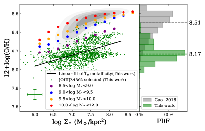
Figure 9: The legends are the same as Figure 6, but green replaces blue. The black solid line still represents the fitting result given by the electronic temperature method data (Equation 9), while green dots and histograms represent the result of the strong line method. The colored solid circles represent the median of metallicity in each M_∗ and $\Sigma_{*}$ bin for interpolation.

Here we use PG16-R-calibrated metallicity, because the applicable metallicity range of M13 calibration is too narrow to include all our spaxels, while the range of PG16 calibration is sufficient to include our sample and G18 sample. The uncertainty of metallicity is also obtained using the same process as Section 2.5. The final uncertainty of PG16-R-calibrated metallicity is $\sim$0.05 dex. For the G18 sample, We re-calculate their metallicity using the R calibration of PG16 to keep consistency.

The new $\Sigma_{*}-Z$ relationship is shown in Figure 9. In addition, we also performed an interpolation fitting on PG16-R-calibrated metallicities of G18 to get a PG16-R-calibrated M${}_{*}-\Sigma_{*}-Z$ relation. The interpolation process is the same as Hwang et al. (2019), so that we can get the expected fitting value of PG16 metallicity ($Z_{\rm fit,PG16}$) under a given M_∗ and $\Sigma_{*}$. The result of interpolation is shown in the colored solid circles in the figure, and the standard deviation between our interpolation result and the observation of G18 is 0.07 dex. Since the statistical uncertainties arising from the emission line measurements are much smaller than the systematic uncertainty (0.049 dex) of the calibration, the error bar of the metallicity is replaced by the systematic uncertainty of the adopted calibration. We can see that after switching to the strong line method, the $\Sigma_{*}-Z$ relation still exists, and it moves down. The median metallicity of the $T_{\rm e}$ method is 8.22, while the PG16 method is 8.17. Under this method, only 64 spaxels ($\sim$3.8%) are within the 1$\sigma$ dispersion of the local MZR of G18. We can confirm the overall low metallicities of our sample and the existence of the local $\Sigma_{*}-Z$ relationship.

4.2 Comparison with All Star Forming Regions in Sample Galaxies and Other Galaxies with Similar M_∗ Distribution

We have determined that our sample galaxies have low total stellar masses in Section 3.1, and their metallicities are lower than the best fit of G18’s M${}_{*}-\Sigma_{*}-Z$ relation at M_∗=$10^{9}$M_⊙. However it is known that the metallicities of the galaxies of a given total stellar mass show a significant scatter, especially at low masses. We should discuss further and clarify whether the metallicity of the selected regions only are lower in comparison to the metallicities of other regions in the same galaxy, or the metallicities of galaxies as whole from their sample are lower in comparison to other galaxies.

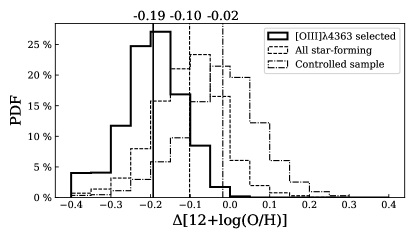
Figure 10: The normalized distribution of metallicity offset ($\Delta$[12+log(O/H)]=$Z_{\rm fit,PG16}(\Sigma_{*}$,M${}_{*})$-$Z_{\rm obs}$). All metallicities are obtained from PG16. Solid border histograms represent the sample we selected by [O iii]$\lambda$4363. Dashed border histograms represent all star-forming spaxels in our sample galaxies. Dash-dot border histograms represent the control sample with similar mass distributions to our sample galaxies. The vertical lines respectively indicate the median of the corresponding border style.

Like Section 3.1, we randomly selected 162 galaxies with similar mass distributions to our sample galaxies from MaNGA to make a control sample, and the O3N2 method (PG16) is also used to calculate their metallicities. In order to verify whether the metallicity is deviated from the normal star-forming sequence, we compare the metallicity of these samples with the interpolated M${}_{*}-\Sigma_{*}-Z$ relation of G18 ($Z_{\rm fit,PG16}(\Sigma_{*}$, M${}_{*})$) in Section 4.1, defining the metallicity offset, $\Delta$[12+log(O/H)]=$Z_{\rm fit,PG16}(\Sigma_{*}$,M${}_{*})$-$Z_{\rm obs}$. The results are shown in Figure 10. The median of [O iii]$\lambda$4363 selected spaxels is -0.19, all star-forming spaxels is -0.10, and control sample is -0.02. This means that not only the metallicity of our [O iii]$\lambda$4363 selected sample are lower than other star-forming regions in their host galaxies, but also the metallicities of these host galaxies are also entirely lower than other galaxies with similar M_∗. Low metallicity is not only a local characteristic, but also a characteristic of the galaxy as a whole. Combined with the above results in 3.1, it shows that the appearance of these metal-poor regions is related to the particularity of the entire galaxy. We should notice that the selection effects caused by flux limits of auroral emission lines may contribute to those results, we leave this consideration for future work when larger sample become avaliable.

4.3 ALM Region and Merger

In Section 3.2, Figures 6 and 9, we have found that our [O iii]$\lambda$4363 selected metal-poor sample are not located at the low-metallicity end of the $\Sigma_{*}-Z$ relationship of normal star-forming regions. They seem to be ALM regions, selected by their significantly lower (about 0.14 dex) observed metallicities compared to the expected ones given $\Sigma_{*}$ and the $\Sigma_{*}-Z$ relation, in Hwang et al. (2019). These authors found that ALM regions tend to exist in less massive and disturbed galaxies. They also estimated the ages of these ALM regions to be a few hundred Myr. Here we use [O iii]$\lambda$4363 emission line to select metal-poor sample to get the more accurate metallicities than strong line method. In our [O iii]$\lambda$4363 selected metal-poor sample, the $t_{*}$ are also between 100 Myr and 1 Gyr ($\log\langle t_{*}\rangle\sim 8.0-9.0$). The distribution of P(merger) shown in the right panel of Figure 3 also shows that our galaxies are likely to experience mergers or interactions compared to the controlled sample. These characteristics are highly consistent with the ALM regions selected by Hwang et al. (2019).

Since the P(merger) from DL catalog is the result of batch processing, it only gives a statistical merging probability. In fact, whether the merger is true requires further inspection, so we check our galaxies one by one. We review the images and spectra of each galaxy and its surrounding galaxies which may be merging objects. Our inspection finds that 11 of the 52 galaxies in our sample have nearby galaxies confirmed by spectral redshifts, of which 6 galaxies (plate-ifu=8566-3704, 8455-9101, 8241-6101, 8139-12702, 9881-9102, and 9194-12701) are within the field of view of the MaNGA IFU, and 3 galaxies (9509-3702, 8715-12704, and 8452-1902) are within 1′. In addition, the neighbors of 3 galaxies (8548-3702, 8553-12703, and 8325-12702) have no spectral redshift but are within the uncertainty of their photometric redshifts. Therefore, a total of 12 galaxies may be merging galaxies, accounting for 23.1% of our sample. Therefore, the results of both the DL catalog and the spectral inspection confirm that our sample has a greater merger ratio than the normal SFGs. Merger and interaction can trigger gas inflow and star formation, and the inflow of metal-poor gas will dilute the metal-rich ISM and form new metal-poor stars. (Kunth & Östlin, 2000), so we can conclude that the interaction is closely related to these metal-poor regions.

5 Conclusion

In this work, we make use of the MaNGA data from the SDSS DR15 to investigate the $\Sigma_{*}-\Sigma_{\rm SFR}$ and $\Sigma_{*}-Z$ relationships. We select 1698 spaxels from 52 galaxies with reliable [O iii]$\lambda$4363 observation. We calculate their local metallicities with the $T_{\rm e}$ method. We have got the following conclusions:

1. There is a local $\Sigma_{*}-\Sigma_{\rm SFR}$ relationship and $\Sigma_{*}-Z$ relationship in the [O iii]$\lambda$4363 emission line selected regions. Among them, in the $\Sigma_{*}-\Sigma_{\rm SFR}$ relationship, our SFR is higher overall (99.4% are outside 1$\sigma$ of SFMS in G18), and in the $\Sigma_{*}-Z$ relationship, our metallicity is lower overall (80.5% are outside 1$\sigma$), and this is not caused by the FMR.

2. The regions we selected have young stars ($<$ 1 Gyr) and their stellar metallicities are also lower ($\sim$ 1% Z_⊙). The $t_{*}$ derived by SED fitting is consistent with the estimated age of the ALM regions reported in Hwang et al. (2019).

3. Most of the galaxies in the selected region are star-forming galaxies with low mass ($\sim$ 10⁹ M_⊙). These galaxies are late in morphology and have a high merging ratio, reflecting that the metal-poor star-forming regions may be related to interactions. The inflow of metal-poor gas may dilute the interstellar medium and form new metal-poor stars in these galaxies during interaction.

However, we do not find a direct evidence for the inflow of metal-poor gas and the relation between merger and gas inflow. How the interaction affects the metallicity of galaxies remains to be further studied.

Appendix A Comparison of Our Results and DAP

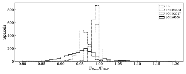
Figure 11: The distribution of the ratio of the flux values of some emission lines (H$\alpha$, [N ii], [O ii]and [O i]) we measured to the flux values provided by DAP at the same spaxel.

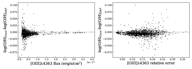
Figure 12: The difference between our metallicity and DAP-flux-based metallicity as the function of [O iii]4363 flux and the relative error.

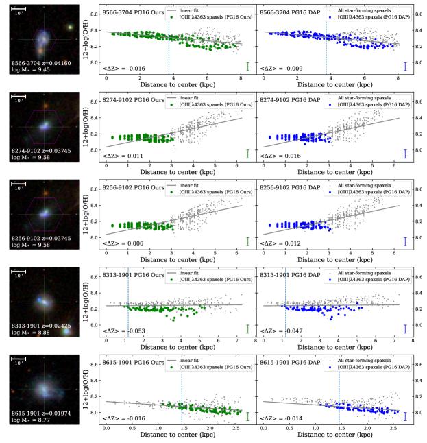
Figure 13: Same as Figure 1, but the flux measurements of the right column are from DAP.

Here we provide a comparison between the results measured by us and provided by DAP. Figure 11 shows the ratio of fluxes of some emission lines. The PG16-based differences between ours and DAP as functions of [O iii]$\lambda$4363 flux and [O iii]$\lambda$4363 relative error are shown in Figure 12. The flux and error here are before the intrinsic dust extinction correction. Figure 13 shows the metallicity profile measured by our fitting and DAP along radius of the first 4 galaxies which have already been shown in Figure 1.

Since the emission lines we compared are all strong emission lines, it cannot prove that the measurement of the weaker emission lines ([O iii]$\lambda$4363) is accurate. However, [O iii]$\lambda$4363 is not measured by DAP, we can estimate its accuracy of fitting through [O i]$\lambda$6300, whose flux is the same magnitude as [O iii]$\lambda$4363’s. The mean flux of [O iii]$\lambda$4363 of our sample is $\sim$0.49$\times$10^-17erg/s/cm², and the mean flux of [O i]$\lambda$6300 is $\sim$1.17$\times$10^-17erg/s/cm². The mean relative difference of [O i]$\lambda$6300 measurement is only $\sim$6%. Therefore, from Figure 11 and 13, we can conclude that our measurement is reliable compared to DAP.

We also calculate the differences between two observations of the same galaxy (8274-9102 and 8256-9102), and they are shown in Figure 14.

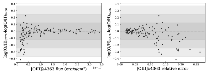
Figure 14: Same as Figure 12, but the difference become the T_e-based metallicity difference between 8274-9102 and 8256-9102. The typical metallicity uncertainty ($\sim$0.12dex) of one, two and three times is indicated by shading of different depths.

Appendix B Images of Other Sample Galaxies

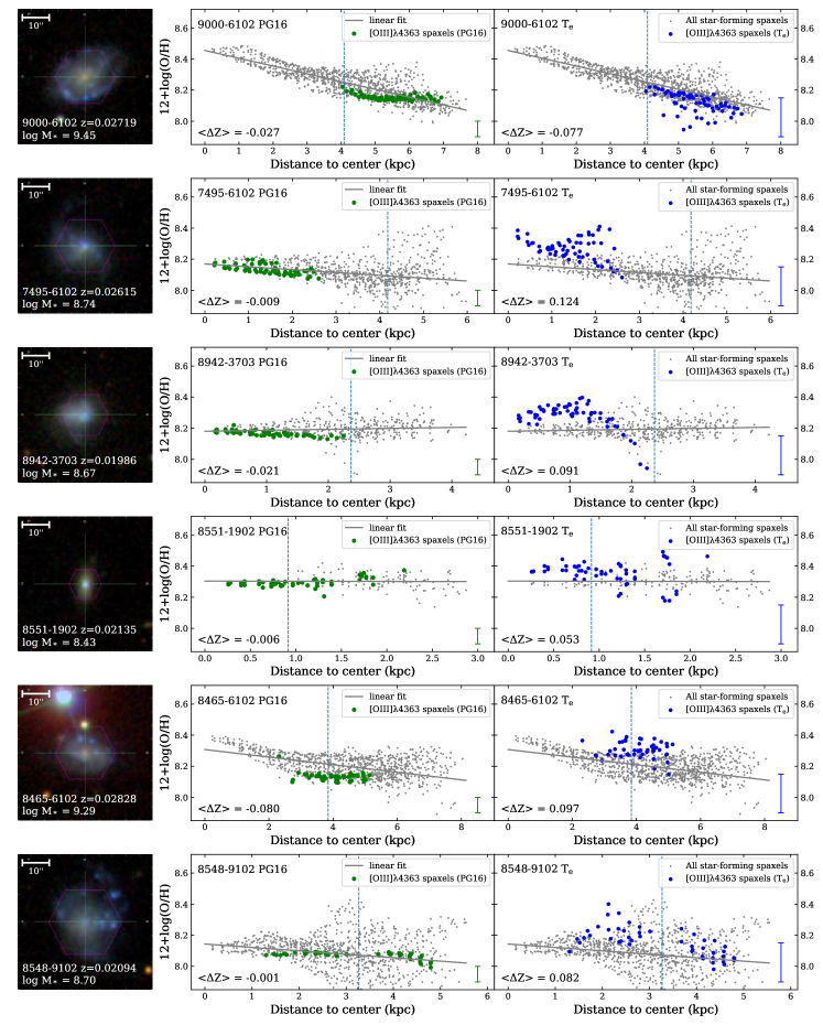
Figure 15: Same as Figure 1, but the galaxies are ranked 5th to 10th in descending order of spaxels.

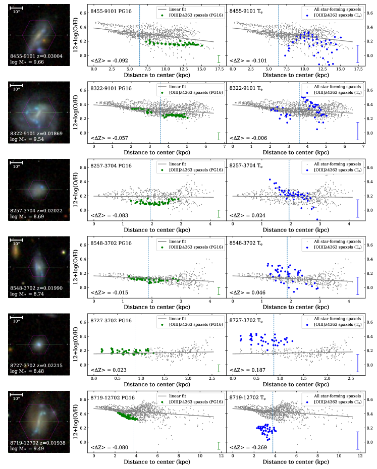
Figure 16: Same as Figure 1, but the galaxies are ranked 11th to 16th in descending order of spaxels.

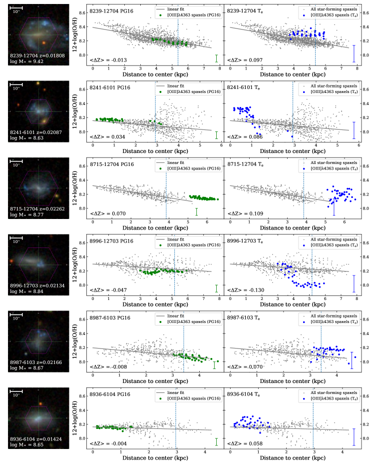
Figure 17: Same as Figure 1, but the galaxies are ranked 17th to 22nd in descending order of spaxels.

References

- Aguado et al. (2019) Aguado, D. S., Ahumada, R., Almeida, A., et al. 2019, ApJS, 240, 23, doi: 10.3847/1538-4365/aaf651
- Aller (1984) Aller, L. H. 1984, Physics of thermal gaseous nebulae, doi: 10.1007/978-94-010-9639-3
- Baldwin et al. (1981) Baldwin, J. A., Phillips, M. M., & Terlevich, R. 1981, PASP, 93, 5, doi: 10.1086/130766
- Barrera-Ballesteros et al. (2016) Barrera-Ballesteros, J. K., Heckman, T. M., Zhu, G. B., et al. 2016, MNRAS, 463, 2513, doi: 10.1093/mnras/stw1984
- Belfiore et al. (2019) Belfiore, F., Westfall, K. B., Schaefer, A., et al. 2019, AJ, 158, 160, doi: 10.3847/1538-3881/ab3e4e
- Blanton et al. (2011) Blanton, M. R., Kazin, E., Muna, D., Weaver, B. A., & Price-Whelan, A. 2011, AJ, 142, 31, doi: 10.1088/0004-6256/142/1/31
- Blanton et al. (2017) Blanton, M. R., Bershady, M. A., Abolfathi, B., et al. 2017, AJ, 154, 28, doi: 10.3847/1538-3881/aa7567
- Bruzual & Charlot (2003) Bruzual, G., & Charlot, S. 2003, MNRAS, 344, 1000, doi: 10.1046/j.1365-8711.2003.06897.x
- Bundy et al. (2015) Bundy, K., Bershady, M. A., Law, D. R., et al. 2015, ApJ, 798, 7, doi: 10.1088/0004-637X/798/1/7
- Calzetti et al. (2000) Calzetti, D., Armus, L., Bohlin, R. C., et al. 2000, ApJ, 533, 682, doi: 10.1086/308692
- Cano-Díaz et al. (2016) Cano-Díaz, M., Sánchez, S. F., Zibetti, S., et al. 2016, ApJ, 821, L26, doi: 10.3847/2041-8205/821/2/L26
- Cardelli et al. (1989) Cardelli, J. A., Clayton, G. C., & Mathis, J. S. 1989, ApJ, 345, 245, doi: 10.1086/167900
- Chabrier (2003) Chabrier, G. 2003, PASP, 115, 763, doi: 10.1086/376392
- Chen et al. (2020) Chen, G., Zhang, H.-X., Kong, X., et al. 2020, The Astrophysical Journal, 895, 146, doi: 10.3847/1538-4357/ab8cc2
- Cid Fernandes et al. (2005) Cid Fernandes, R., Mateus, A., Sodré, L., Stasińska, G., & Gomes, J. M. 2005, MNRAS, 358, 363, doi: 10.1111/j.1365-2966.2005.08752.x
- Domínguez Sánchez et al. (2018) Domínguez Sánchez, H., Huertas-Company, M., Bernardi, M., Tuccillo, D., & Fischer, J. L. 2018, MNRAS, 476, 3661, doi: 10.1093/mnras/sty338
- Drory et al. (2015) Drory, N., MacDonald, N., Bershady, M. A., et al. 2015, AJ, 149, 77, doi: 10.1088/0004-6256/149/2/77
- Fischer et al. (2018) Fischer, J.-L., Domínguez Sánchez, H., & Bernardi, M. 2018, Monthly Notices of the Royal Astronomical Society, 483, 2057, doi: 10.1093/mnras/sty3135
- Gao et al. (2018) Gao, Y., Wang, E., Kong, X., et al. 2018, ApJ, 868, 89, doi: 10.3847/1538-4357/aae9f1
- Gao et al. (2017) Gao, Y.-L., Lian, J.-H., Kong, X., et al. 2017, Research in Astronomy and Astrophysics, 17, 041, doi: 10.1088/1674-4527/17/5/41
- Hummer & Storey (1987) Hummer, D. G., & Storey, P. J. 1987, MNRAS, 224, 801, doi: 10.1093/mnras/224.3.801
- Hwang et al. (2019) Hwang, H.-C., Barrera-Ballesteros, J. K., Heckman, T. M., et al. 2019, ApJ, 872, 144, doi: 10.3847/1538-4357/aaf7a3
- Izotov et al. (2006) Izotov, Y. I., Stasińska, G., Meynet, G., Guseva, N. G., & Thuan, T. X. 2006, A&A, 448, 955, doi: 10.1051/0004-6361:20053763
- Kauffmann et al. (2003a) Kauffmann, G., Heckman, T. M., Tremonti, C., et al. 2003a, MNRAS, 346, 1055, doi: 10.1111/j.1365-2966.2003.07154.x
- Kauffmann et al. (2003b) Kauffmann, G., Heckman, T. M., White, S. D. M., et al. 2003b, MNRAS, 341, 33, doi: 10.1046/j.1365-8711.2003.06291.x
- Kennicutt (1998) Kennicutt, Robert C., J. 1998, ARA&A, 36, 189, doi: 10.1146/annurev.astro.36.1.189
- Kewley et al. (2019) Kewley, L. J., Nicholls, D. C., & Sutherland, R. S. 2019, ARA&A, 57, 511, doi: 10.1146/annurev-astro-081817-051832
- Kunth & Östlin (2000) Kunth, D., & Östlin, G. 2000, A&A Rev., 10, 1, doi: 10.1007/s001590000005
- Law et al. (2016) Law, D. R., Cherinka, B., Yan, R., et al. 2016, AJ, 152, 83, doi: 10.3847/0004-6256/152/4/83
- Lequeux et al. (1979) Lequeux, J., Peimbert, M., Rayo, J. F., Serrano, A., & Torres-Peimbert, S. 1979, A&A, 500, 145
- Liu et al. (2018) Liu, Q., Wang, E., Lin, Z., et al. 2018, ApJ, 857, 17, doi: 10.3847/1538-4357/aab3d5
- López-Sánchez et al. (2011) López-Sánchez, Á. R., Mesa-Delgado, A., López-Martín, L., & Esteban, C. 2011, MNRAS, 411, 2076, doi: 10.1111/j.1365-2966.2010.17847.x
- Ly et al. (2014) Ly, C., Malkan, M. A., Nagao, T., et al. 2014, ApJ, 780, 122, doi: 10.1088/0004-637X/780/2/122
- Mannucci et al. (2010) Mannucci, F., Cresci, G., Maiolino, R., Marconi, A., & Gnerucci, A. 2010, MNRAS, 408, 2115, doi: 10.1111/j.1365-2966.2010.17291.x
- Marino et al. (2013) Marino, R. A., Rosales-Ortega, F. F., Sánchez, S. F., et al. 2013, A&A, 559, A114, doi: 10.1051/0004-6361/201321956
- Markwardt (2009) Markwardt, C. B. 2009, in Astronomical Society of the Pacific Conference Series, Vol. 411, Astronomical Data Analysis Software and Systems XVIII, ed. D. A. Bohlender, D. Durand, & P. Dowler, 251. https://arxiv.org/abs/0902.2850
- Meert et al. (2014) Meert, A., Vikram, V., & Bernardi, M. 2014, Monthly Notices of the Royal Astronomical Society, 446, 3943, doi: 10.1093/mnras/stu2333
- Nair & Abraham (2010) Nair, P. B., & Abraham, R. G. 2010, ApJS, 186, 427, doi: 10.1088/0067-0049/186/2/427
- Pettini & Pagel (2004) Pettini, M., & Pagel, B. E. J. 2004, MNRAS, 348, L59, doi: 10.1111/j.1365-2966.2004.07591.x
- Pilyugin & Grebel (2016) Pilyugin, L. S., & Grebel, E. K. 2016, MNRAS, 457, 3678, doi: 10.1093/mnras/stw238
- Pilyugin et al. (2009) Pilyugin, L. S., Mattsson, L., Vílchez, J. M., & Cedrés, B. 2009, MNRAS, 398, 485, doi: 10.1111/j.1365-2966.2009.15182.x
- Pilyugin et al. (2010) Pilyugin, L. S., Vílchez, J. M., & Thuan, T. X. 2010, ApJ, 720, 1738, doi: 10.1088/0004-637X/720/2/1738
- Rosales-Ortega et al. (2010) Rosales-Ortega, F. F., Kennicutt, R. C., Sánchez, S. F., et al. 2010, MNRAS, 405, 735, doi: 10.1111/j.1365-2966.2010.16498.x
- Rosales-Ortega et al. (2012) Rosales-Ortega, F. F., Sánchez, S. F., Iglesias-Páramo, J., et al. 2012, ApJ, 756, L31, doi: 10.1088/2041-8205/756/2/L31
- Salim et al. (2007) Salim, S., Rich, R. M., Charlot, S., et al. 2007, ApJS, 173, 267, doi: 10.1086/519218
- Sánchez et al. (2012) Sánchez, S. F., Kennicutt, R. C., Gil de Paz, A., et al. 2012, A&A, 538, A8, doi: 10.1051/0004-6361/201117353
- Schlegel et al. (1998) Schlegel, D. J., Finkbeiner, D. P., & Davis, M. 1998, ApJ, 500, 525, doi: 10.1086/305772
- Tremonti et al. (2004) Tremonti, C. A., Heckman, T. M., Kauffmann, G., et al. 2004, ApJ, 613, 898, doi: 10.1086/423264
- Westfall et al. (2019) Westfall, K. B., Cappellari, M., Bershady, M. A., et al. 2019, AJ, 158, 231, doi: 10.3847/1538-3881/ab44a2