STATUS: arXiv pre-print

(1.25in,2in) FMM-accelerated solvers for the Laplace-Beltrami
problem on complex surfaces in three dimensions

Dhwanit Agarwal
Oden Institute, University of Texas at Austin
Austin, TX, 78712
dhwanit@oden.utexas.edu

Michael O’Neil
Courant Institute, NYU
New York, NY 10012
oneil@cims.nyu.edu

Manas Rachh
Center for Computational Mathematics, Flatiron Institute
New York, NY 10010
mrachh@flatironinstitute.org

(1.25in,7in)

Abstract

The Laplace-Beltrami problem on closed surfaces embedded in three dimensions arises in many areas of physics, including molecular dynamics (surface diffusion), electromagnetics (harmonic vector fields), and fluid dynamics (vesicle deformation). Using classical potential theory, the Laplace-Beltrami operator can be pre-/post-conditioned with an integral operator whose kernel is translation invariant, resulting in well-conditioned Fredholm integral equations of the second-kind. These equations have the standard $1/r$ kernel from potential theory, and therefore the equations can be solved rapidly and accurately using a combination of fast multipole methods (FMMs) and high-order quadrature corrections. In this work we detail such a scheme, presenting two alternative integral formulations of the Laplace-Beltrami problem, each of whose solution can be obtained via FMM acceleration. We then present several applications of the solvers, focusing on the computation of what are known as harmonic vector fields, relevant for many applications in electromagnetics. A battery of numerical results are presented for each application, detailing the performance of the solver in various geometries.

Keywords: Nyström method, Laplace-Beltrami, harmonic vector field, fast multipole method, potential theory.

1 Introduction

The Laplace-Beltrami problem along surfaces in three dimensions appears in many fields, including plasma physics [31], fluid mechanics [35, 39], electromagnetics [11, 13, 14, 32], surface diffusion, pattern formation [23, 34], and computational geometry [26]. In general, the Laplace-Beltrami operator is a second-order variable coefficient elliptic operator whose behavior is highly dependent on the nature of the surface on which it is defined. Its eigenfunctions are useful in describing band-limited functions defined along the associated manifold or surface, and more generally, the related harmonic vector fields provide a basis for important classes of functions appearing in electromagnetics (e.g. non-radiating currents, etc.).

To describe the problem, suppose that $\Gamma$ is at least a twice-differentiable surface without boundary embedded in $\mathbb{R}^{3}$. Let $\nabla_{\Gamma}$ denote the intrinsic surface gradient, and let its adjoint acting on the space of continuously differentiable $\mathbb{L}^{2}$ tangential vector fields on the boundary, denoted by $\nabla_{\Gamma}\cdot$, be the intrinsic surface divergence. Given a mean-zero function $f$ defined along $\Gamma$, the Laplace-Beltrami problem is to find a mean-zero function $u$ satisfying $\Delta_{\Gamma}u=f$, where $\Delta_{\Gamma}$ is the Laplace-Beltrami operator defined as $\Delta_{\Gamma}=\nabla_{\Gamma}\cdot\nabla_{\Gamma}$. The mean-zero condition on $f$ and $u$ is required for unique solvability due to a rank-deficiency of the Laplace-Beltrami operator [33, 11, 32].

In many of the applications discussed above, the Laplace-Beltrami problem naturally arises for the computation of the Hodge decomposition of tangential vector fields. Any smooth tangential vector field $\bm{F}$ on the surface $\Gamma$ can be written as

$$\bm{F}=\nabla_{\Gamma}\alpha+\bm{n}\times\nabla_{\Gamma}\beta+\bm{H}\,,$$ (1.1)

where $\alpha$, $\beta$ are smooth functions on $\Gamma$, $\bm{H}$ is a harmonic field satisfying $\nabla_{\Gamma}\cdot\bm{H}=\nabla_{\Gamma}\cdot\bm{n}\times\bm{H}=0$, and $\bm{n}$ is the unit normal to the surface $\Gamma$. The curl free component $\nabla_{\Gamma}\alpha$ and the divergence free component $\bm{n}\times\nabla_{\Gamma}\beta$ can be computed via the solution of the following two Laplace-Beltrami problems:

$$\Delta_{\Gamma}\alpha =\nabla_{\Gamma}\cdot\bm{F},$$ (1.2)

$$\Delta_{\Gamma}\beta =-\nabla_{\Gamma}\cdot(\bm{n}\times\bm{F}).$$

A related problem is that of determining a basis for harmonic vector fields on non-contractible surfaces, which plays a crucial role for several integral representations in computational electromagnetics. On a genus $g$ object, the space of harmonic vector fields forms a $2g$-dimensional vector space. One can compute elements of this basis via the solution of the two Laplace-Beltrami problems above for a randomly generated smooth vector field $\bm{F}$, which with high probability tends to have a non-trivial projection onto the subspace of harmonic vector fields.

Numerical methods for the Laplace-Beltrami problem can be typically classified into two categories. The first category of methods rely on the direct discretization of the differential operator on surface. Examples include finite element methods [2, 5, 7, 10], virtual element methods [3, 16], differencing methods [42], and level set methods [4, 8, 20, 29, 30]. The level set methods differ from the rest of the direct discretizations of the PDE as they rely on using an embedded finite difference grid in the volume $\mathbb{R}^{3}$ to discretize a thickening of the surface.

On the other hand, the other general category of methods is to reformulate the Laplace-Beltrami problem as an integral equation along the surface. For example, on a flat surface the Laplace-Beltrami operator reduces to the standard Laplace operator and therefore the Green’s function is known to be $G(\bm{x})=-\log{|\bm{x}|}/(2\pi)$. This Green’s function $G$ can be used as a parametrix for the fundamental solution to the Laplace-Beltrami operator on surfaces as well [27]. This idea has also been used for the solution of the related Yukawa-Beltrami problem on general surfaces, including surfaces with boundary in [28]. A separation of variables approach, combined with an integral reformulation of an ODE, is presented in [17]; this approach was also shown to be applicable in geometries with edges. An alternate integral equation-based approach is to use the Green’s function of the free-space Laplace equation in three dimensions as either left or right preconditioners for the Laplace-Beltrami problem [33].

In this work, we present a fast multipole method (FMM) accelerated iterative solver for the solution of the Laplace-Beltrami problems on complex three-dimensional surfaces based on the integral formulation presented in [33], and using the locally corrected quadrature approach of [18]. In some respects, this work can be considered Part II of the earlier work [33]. The primary motivation of choosing this approach is two-fold: (1) the resulting integral equations tend to be as well-conditioned as the underlying physical problem (which is quite well-conditioned in this case, in an absolute sense), and (2) since the representation uses layer potentials related to the free space Green’s function in three dimensions, the numerical solver can be coupled to existing optimized FMM libraries [19, 18]. We demonstrate the well-conditioned nature of the integral equation through a battery of numerical experiments, each of which incorporates a high-order representation of the surface and high-order quadratures. We also show the importance of what we refer to as numerical second-kindness when discretizing the integral equation using locally corrected quadrature methods. These methods rely on the accurate computation of the principal-value part of the layer potentials in the representation. In particular, while there are several equivalent integral formulations of the same PDE on the surface, we show that the formulation which explicitly handles the identity term of the integral equation tends to be the most stable (from a numerical point of view). Lastly, with the acceleration provided by FMMs, our integral formulation can be used to compute a basis for harmonic vector fields in relatively high-genus geometries.

The rest of the paper is organized in follows. In Section 2, we describe the Laplace-Beltrami problem. In Section 3, we review the integral equation formulation presented in [33], and in Section 4, we review a high order FMM-accelerated iterative solver. In Section 5, we discuss an application of the solver to the computation of a basis for harmonic vector fields on non-contractible surfaces. In Section 6, we present several numerical examples to demonstrate the efficiency of our approach, including a discussion on the importance of numerical second-kindness. Finally, in Section 7, we conclude by discussing avenues for future research.

2 The Laplace-Beltrami problem

The Laplace-Beltrami operator, also known as the surface Laplacian, is the generalization of the Laplace operator to general (smooth) manifolds. In this work, we will focus on smooth surfaces embedded in three dimensions. Suppose $\Gamma\subset\mathbb{R}^{3}$ is an oriented surface with at least two continuous derivatives, and let $\bm{x}(u,v):D\subset\mathbb{R}^{2}\to\mathbb{R}^{3}$ denote a local parametrization of $\Gamma$. The first fundamental form, or equivalently the metric tensor at $\bm{x}(u,v)$, is given by

$$g=\begin{bmatrix}g_{11}&g_{12}\\ g_{21}&g_{22}\end{bmatrix}=\begin{bmatrix}\partial_{u}\bm{x}\cdot\partial_{u}\bm{x}&\partial_{u}\bm{x}\cdot\partial_{v}\bm{x}\\ \partial_{v}\bm{x}\cdot\partial_{u}\bm{x}&\partial_{v}\bm{x}\cdot\partial_{v}\bm{x}\end{bmatrix},$$ (2.1)

where $\partial_{u}\bm{x}$ and $\partial_{v}\bm{x}$ are abbreviations for $\frac{\partial\bm{x}}{\partial u}$ and $\frac{\partial\bm{x}}{\partial v}$, respectively, and are tangent vectors to the surface at $\bm{x}\in\Gamma$. The unit normal at $\bm{x}$ can written as

$$\bm{n}(\bm{x})=\frac{\partial_{u}\bm{x}\times\partial_{v}\bm{x}}{|\partial_{u}\bm{x}\times\partial_{v}\bm{x}|}.$$ (2.2)

The unit vectors in the directions of $\partial_{u}\bm{x}$, $\partial_{v}\bm{x}$, and $\bm{n}(\bm{x})$ form a local coordinate system (not necessarily orthogonal) at each point $\bm{x}\in\Gamma$.

Next, suppose that $\bm{F}$ is a smooth tangential vector field defined along $\Gamma$ and is expressed in terms of the local tangent vectors $\partial_{u}\bm{x}$, $\partial_{v}\bm{x}$ as

$$\bm{F}(u,v)=F_{1}\partial_{u}\bm{x}+F_{2}\partial_{v}\bm{x}\,.$$ (2.3)

The surface divergence of $\bm{F}$, denoted by $\nabla_{\Gamma}\cdot\bm{F}$, is then [32, 15] given by

$$\nabla_{\Gamma}\cdot\bm{F}=\frac{1}{\sqrt{|g|}}\left(\partial_{u}\left(\sqrt{|g|}F_{1}\right)+\partial_{v}\left(\sqrt{|g|}F_{2}\right)\right)\,,$$ (2.4)

where $|g|$ is the determinant of the metric tensor $g$. The surface gradient operator $\nabla_{\Gamma}$, formally defined as the adjoint of the surface divergence operator on the space of $\mathbb{L}^{2}$ functions with respect to the induced metric on $\Gamma$, is given by

$$\nabla_{\Gamma}\psi=\left(g^{11}\partial_{u}\psi+g^{12}\partial_{v}\psi\right)\partial_{u}\bm{x}+\left(g^{21}\partial_{u}\psi+g^{22}\partial_{v}\psi\right)\partial_{v}\bm{x}\,,$$ (2.5)

where $\psi=\psi(u,v)$ is a scalar function defined on $\Gamma$ and $g^{ij}$ denote the components of the inverse of the metric tensor, denoted by $g^{-1}$.

The Laplace-Beltrami operator is then defined as $\Delta_{\Gamma}=\nabla_{\Gamma}\cdot\nabla_{\Gamma}$, and is explicitly given by the expression

$$\Delta_{\Gamma}\psi=\frac{1}{\sqrt{|g|}}\left(\partial_{u}\left[\sqrt{|g|}\left(g^{11}\partial_{u}\psi+g^{12}\partial_{v}\psi\right)\right]+\partial_{v}\left[\sqrt{|g|}\left(g^{21}\partial_{u}\psi+g^{22}\partial_{v}\psi\right)\right]\right).$$ (2.6)

The standard Laplace-Beltrami problem is to solve the following PDE for $\psi$ along $\Gamma$,

$$\Delta_{\Gamma}\psi=f,$$ (2.7)

where $f$ is a given function. Conditions on the regularity required in $f$, and the subsequent regularity obtained in $\psi$ have been studied in [36, 22, 11, 17]. We will assume that all functions and surfaces are sufficiently smooth so as to obtain high order accuracy in the subsequently numerical examples.

As is clear, the Laplace-Beltrami operator maps constant functions along $\Gamma$ to zero. Thus, the equation (2.7) is rank-one deficient [21, 38] (and formally self-adjoint). The following lemma [36, 33] summarizes a classical result regarding the well-posedness of the above Laplace-Beltrami problem.

Lemma 1.

Let $\Gamma$ be a smooth, closed, and orientable boundary. Along $\Gamma$, the Laplace-Beltrami operator is uniquely invertible as a map from $\mathbb{M}_{0}\to\mathbb{M}_{0}$, the space of mean-zero functions defined on $\Gamma$,

$$\mathbb{M}_{0}=\left\{\psi\,:\,\int_{\Gamma}\psi\,da=0\right\}\,.$$ (2.8)

Indeed, if the function $f$ defined along $\Gamma$ has mean zero, then there exists a unique mean-zero solution, $\psi$, to the Laplace-Beltrami problem $\Delta_{\Gamma}\psi=f$.

3 Integral equation formulations

In this section, we review an equivalent well-conditioned second-kind integral equation for the solution of the Laplace-Beltrami problem. This formulation relies on preconditioning the Laplace-Beltrami operator on both the left and right using the Laplace single layer potential. The resulting Fredholm operator can be expressed in terms of standard layer potentials for the free space Laplace equation in three dimensions. Before describing this formulation, we first define the relevant layer potentials used in the formulation. The Green’s function $G$ for Laplace’s equation in three dimensions is given by

$$G(\bm{x},\bm{y})=\frac{1}{4\pi|\bm{x}-\bm{y}|}\,.$$ (3.1)

The single and double layer potentials are then given by:

$$\mathcal{S}[\sigma](\bm{x}) =\int_{\Gamma}G(\bm{x},\bm{y})\,\sigma(\bm{y})\,da,$$ (3.2)

$$\mathcal{D}[\mu](\bm{x}) =\int_{\Gamma}\left(\nabla_{\bm{y}}G(\bm{x},\bm{y})\cdot\bm{n}(\bm{y})\right)\mu(\bm{y})\,da.$$

When the target point $\bm{x}$ lies on $\Gamma$, the integral defining the double layer should be interpreted in a principal value sense. For smooth surfaces $\Gamma$, both $\mathcal{S}$ and $\mathcal{D}$ are compact operators as maps from $\mathbb{L}^{2}(\Gamma)\to\mathbb{L}^{2}(\Gamma)$. Related to the single and double layer potentials are the restrictions of their normal derivatives to $\Gamma$ given by

$$\mathcal{S}^{\prime}[\sigma](\bm{x}) =\bm{n}(\bm{x})\cdot\nabla\int_{\Gamma}G(\bm{x},\bm{y})\sigma(\bm{y})\,da,$$ (3.3)

$$\mathcal{D}^{\prime}[\mu](\bm{x}) =\int_{\Gamma}\bm{n}(\bm{x})\cdot\nabla_{\bm{x}}\nabla_{\bm{y}}G(\bm{x},\bm{y})\cdot\bm{n}(\bm{y})\mu(\bm{y})\,da.$$

The integral defining $\mathcal{S}^{\prime}$ is to be interpreted in a principal value sense, and that for $\mathcal{D}^{\prime}$ is to be interpreted in a finite-part sense [25, 32]. The operator $\mathcal{S}^{\prime}$ is also a compact operator on $\mathbb{L}^{2}(\Gamma)$, whereas $\mathcal{D}^{\prime}$ is a hypersingular operator.

Finally, let $\mathcal{S}^{\prime\prime}$ denote the restriction of the second normal derivative of $\mathcal{S}$ to $\Gamma$ given by:

$$\mathcal{S}^{\prime\prime}[\sigma](\bm{x})=\int_{\Gamma}\left(\bm{n}(\bm{x})\cdot\nabla_{\bm{x}}\nabla_{\bm{x}}G(\bm{x},\bm{y})\cdot\bm{n}(\bm{x})\right)\sigma(\bm{y})\,da,$$ (3.4)

where, as for the integral defining $\mathcal{D}^{\prime}$, the integral should be interpreted in a finite-part sense [25, 32, 33]. It can be shown that the difference operator $\mathcal{S}^{\prime\prime}+\mathcal{D}^{\prime}$ is a compact operator on $\mathbb{L}^{2}(\Gamma)$ [32], as the dominant singularities in the integrand cancel each other out.

We now review two equivalent second-kind boundary integral formulations for the solution of the Laplace-Beltrami equation (2.7) as presented in [33]. One formulation is to represent the solution $\psi=\mathcal{S}[\sigma]$, where $\sigma$ is an unknown density and precondition to equation (2.7) using $\mathcal{S}$, i.e. solve

$$\mathcal{S}\Delta_{\Gamma}\mathcal{S}[\sigma]=\mathcal{S}[f]\,.$$ (3.5)

Using Calderón identities, the equation above can be rewritten as

$$-\frac{\sigma}{4}+\mathcal{D}^{2}[\sigma]-\mathcal{S}\left(\mathcal{S}^{\prime\prime}+\mathcal{D}^{\prime}+2H\mathcal{S}^{\prime}\right)[\sigma]=\mathcal{S}[f]\,,$$ (3.6)

where $H$ is the mean curvature along $\Gamma$. The above equation still has a one dimensional null-space which is related to constant functions comprising the null-space of the Laplace Beltrami problem. To impose the integral equation on the space of mean-zero functions, we instead solve the integral equation

$$-\frac{\sigma}{4}+\mathcal{D}^{2}[\sigma]-\mathcal{S}\left(\mathcal{S}^{\prime\prime}+\mathcal{D}^{\prime}+2H\mathcal{S}^{\prime}\right)[\sigma]+\mathcal{SWS}[\sigma]=\mathcal{S}[f]\,,$$ (3.7)

where $\mathcal{W}$ is the operator given by

$$\mathcal{W}[\sigma]=\frac{1}{|\Gamma|}\int_{\Gamma}\sigma\,da\,.$$ (3.8)

If $f$ is a mean-zero function in $\mathbb{L}^{2}(\Gamma)$, then there exists a unique solution $\sigma$ in $\mathbb{L}^{2}(\Gamma)$ which satisfies Equation 3.7, along with $\int_{\Gamma}\mathcal{S}[\sigma]\,da=0$. Furthermore, $\psi=\mathcal{S}[\sigma]$ is the unique mean-zero solution to the Laplace-Beltrami problem $\Delta_{\Gamma}\psi=f$.

An alternate integral formulation is to instead represent $\psi=\mathcal{S}^{2}[\sigma]$, where $\sigma$ as before is an unknown density and solve

$$\Delta_{\Gamma}\mathcal{S}^{2}[\sigma]=f\,,$$ (3.9)

which using Calderón identities, can be rewritten as

$$-\frac{\sigma}{4}+(\mathcal{S}^{\prime})^{2}[\sigma]-(\mathcal{S}^{\prime\prime}+\mathcal{D}^{\prime}+2H\mathcal{S}^{\prime})\mathcal{S}[\sigma]=f\,.$$ (3.10)

The integral equation above has a similar one-dimensional null space issue as Equation 3.6, which can be addressed using the averaging operator $\mathcal{W}$ by instead solving

$$-\frac{\sigma}{4}+(\mathcal{S}^{\prime})^{2}[\sigma]-(\mathcal{S}^{\prime\prime}+\mathcal{D}^{\prime}+2H\mathcal{S}^{\prime})\mathcal{S}[\sigma]+\mathcal{W}\mathcal{S}^{2}[\sigma]=f\,.$$ (3.11)

Again, if $f$ is a mean-zero function in $\mathbb{L}^{2}(\Gamma)$, then there exists a unique solution $\sigma$ in $\mathbb{L}^{2}(\Gamma)$ which satisfies Equation 3.11, along with $\int_{\Gamma}\mathcal{S}^{2}[\sigma]\,da=0$. Furthermore, $\psi=\mathcal{S}^{2}[\sigma]$ is the unique mean-zero solution the Laplace-Beltrami problem $\Delta_{\Gamma}\psi=f$. A proof of these results can be found in [33].

4 FMM-accelerated solvers

In this section, we describe the details of a numerical solver for integral equation formulations of the Laplace-Beltrami problem. For this, we first briefly recap the FMM-accelerated locally corrected quadrature approach of [18]. For simplicity, consider a second-kind integral equation of the form

$$\sigma(\bm{x})+\int_{\Gamma}K(\bm{x},\bm{x}^{\prime})\,\sigma(\bm{x}^{\prime})\,da(\bm{x}^{\prime})=f(\bm{x})\,\quad\bm{x}\in\Gamma\,,$$ (4.1)

where $K(\bm{x},\bm{x}^{\prime})$ is either $G(\bm{x},\bm{x}^{\prime})$ or one its directional derivatives. Suppose that the surface $\Gamma$ is represented via a disjoint union of patches $\Gamma_{j}$ so that $\Gamma=\cup_{j=1}^{N_{\textrm{patches}}}\Gamma_{j}$, and that each patch $\Gamma_{j}$ is parametrized by a non-degenerate chart $\bm{X}^{j}:T_{0}\to\Gamma_{j}$, where $T_{0}$ is the standard simplex given by

$$T_{0}=\{(u,v):u\geq 0\,,v\geq 0\,,u+v\leq 1\}\subset\mathbb{R}^{2}\,.$$

An order $p$ discretization of $\Gamma$ is one where the components of $\bm{X}^{j},\partial_{u}\bm{X}^{j}$, and $\partial_{v}\bm{X}^{j}$ are represented by a polynomial expansion of total degree less than $p$ on $T_{0}$. One way to obtain such a representation is to sample the chart and the derivative information at order $p$ Vioreanu-Rokhlin nodes [41] which are stable interpolation nodes for orthogonal polynomials [6, 24] on $T_{0}$.

Remark 1.

Triangulations of surfaces obtained from CAD or standard meshing packages often tend to be low order and introduce several artificial edges and corners on the discretized surface. In our examples, with the aim of showing high-order convergence, we use the surface smoothing algorithm discussed in [40] to convert these low-order triangulations of complex geometries to arbitrarily high order triangulations of a nearby related $C^{\infty}$ surface. In some of our examples, analytic parameterizations of the domains are known and are used instead of the algorithm of [40]. The algorithm was only applied to complex geometries, such as the multi-holed object in Figure LABEL:fig:g10.

Let $\{\bm{x}_{i},w_{i}\}_{i=1}^{N}$ denote the union of the samples of the charts $\bm{X}^{j}$ at the Vioreanu-Rokhlin nodes of order $p$, and the corresponding quadrature weights for integrating smooth functions on the surface. A Nyström discretization of Equation 4.1 is given by

$$\sigma_{i}+w_{ii}\sigma_{i}+\sum_{j\neq i}w_{ij}K(\bm{x}_{i},\bm{x}_{j})\sigma_{j}=f(\bm{x}_{i})\,,$$ (4.2)

where $\sigma_{i}$ is an approximation for the solution $\sigma(\bm{x}_{i})$, and $w_{ij}$ are target dependent quadrature weights corresponding to a high-order accurate discretization of the integral appearing in equation (4.1). In [18], for targets $\bm{x}_{i}\in\Gamma_{\ell}$, this integral is numerically approximated using a combination of generalized Gaussian quadrature for the contribution of $\Gamma_{\ell}$ to the overall layer potential, adaptive integration for patches $\Gamma_{j}$ which are close to $\bm{x}_{i}$, and target independent oversampled quadratures for all the remaining patches (which all have smooth integrands). For each discretization point $\bm{x}_{i}$, we can split the computational domain as

$$\mathbb{R}^{3}=\textrm{Far}(\bm{x}_{i})\cup\textrm{Near}(\bm{x}_{i}),$$ (4.3)

with $\textrm{Near}(\bm{x}_{i})$ containing $O(1)$ patches, and hence $O(1)$ discretization points.

Let $\{\bm{s}_{i},w^{\textnormal{over}}_{i}\}_{i=1}^{N_{\textnormal{over}}}$ denote the oversampled quadrature nodes and weights for integrating smooth functions on $\Gamma$, then the Nyström discretization in Equation 4.2 takes the form

$$\sigma_{i}+\sum_{j=1}^{n_{i}}w_{ij}\,K(\bm{x}_{i},\bm{y}_{ij})\,\tilde{\sigma}_{ij}+\sum_{\begin{subarray}{c}j=1\\ \bm{s}_{j}\in\textrm{Far}(\bm{x}_{i})\end{subarray}}^{N_{\textnormal{over}}}w^{\textnormal{over}}_{j}\,K(\bm{x}_{i},\bm{s}_{j})\,\tilde{\sigma}_{j}=f(\bm{x}_{i})\,,$$ (4.4)

where $\tilde{\sigma_{j}}$ and $\tilde{\sigma}_{ij}$ correspond to (approximate) interpolated values of $\sigma$ evaluated at $\bm{s}_{j}$ and $\bm{y}_{ij}$, respectively, obtained via implicit local polynomial interpolation of the samples $\sigma_{i}$. The pairs $\{\bm{y}_{ij},w_{ij}\}$ are the quadrature nodes and weights used in the adaptive integration procedure to accurately compute the contribution of the layer potential due to the self panel $\Gamma_{\ell}$ and the associated near panels at the target location $\bm{x}_{i}$. After adding and subtracting the contribution of the oversampled sources in $\textrm{Near}(\bm{x}_{i})$, and then subsequently composing the interpolation matrices to compute $\tilde{\sigma}_{ij}$ and $\tilde{\sigma}_{j}$ in $\textrm{Near}(\bm{x}_{i})$ and the corresponding kernel evaluations, the discretized integral equation in (4.4) can be rewritten as

$$\sigma_{i}+\sum_{\begin{subarray}{c}j=1\\ \bm{x}_{j}\in\textrm{Near}(\bm{x}_{i})\end{subarray}}^{N}\tilde{w}_{ij}\,\sigma_{j}+\sum_{j=1}^{N_{\textnormal{over}}}w^{\textnormal{over}}_{j}\,K(\bm{x}_{i},\bm{s}_{j})\,\tilde{\sigma}_{j}=f(\bm{x}_{i}),$$ (4.5)

where $\tilde{w}_{ij}$ represents an adjusted weight-kernel product obtained from the addition/subtraction procedure. (See [18] for a very detailed discussion of this procedure, which we have very concisely summarized above.)

The rate limiting step for numerically evaluating the layer potential via this procedure is the computation of the local quadrature corrections. However, when using an an iterative algorithm such as GMRES [37] to solve the integral equation, the effective quadrature-kernel weights $\tilde{w}_{ij}$ above are precomputed and stored. Thus the computational cost of generating the quadrature corrections is amortized over the number of GMRES iterations. The memory requirement of this storage scales like $O(N)$ as there are $O(1)$ points in $\textrm{Near}(\bm{x}_{i})$. Since the far field part of the layer potential is computed using a target independent quadrature rule, i.e. the sum over the oversampled sources $\bm{s}$ in (4.5), the corresponding contribution can be computed using standard fast multipole methods [19, 18]. Using this fast layer potential evaluator, we can obtain the solution $\sigma$ in $O(N)$ time if (4.4) is well-conditioned.

The recent release of the FMM3D package allows for the computation of the vector version of FMM sums, i.e., FMM sums with the same kernel, same source and target locations, but with different strength vectors. Let $\bm{s}_{j}$ denote the source locations, $c_{\ell,j}$ denote the charge strengths, and $\bm{v}_{\ell,j}$ denote the dipole vectors, at $N$ sources, $j=1,2,\ldots N$, and $\ell=1,2\ldots n_{d}$ densities, then the vector version of the Laplace FMM computes the potentials $u_{\ell}(\bm{x})$ given by

$$u_{\ell}(\bm{x})=\sum_{j=1}^{N}\frac{c_{\ell,j}}{|\bm{x}-\bm{s}_{j}|}-\bm{v}_{\ell,j}\cdot\nabla_{\bm{x}}\frac{1}{|\bm{x}-\bm{s}_{j}|}\,,\quad\ell=1,2\ldots n_{d}\,,$$ (4.6)

along with the their gradients and hessians (if requested) at a given set of target locations $x=\bm{t}_{i}$, $i=1,2\ldots M$. The vector version of the FMM is (empirically) computationally more efficient than separately calling $n_{d}$ separate FMMs since various density independent quantities can be reused in the FMM algorithm. This feature of the FMM can be used for the more efficient computation of multiple operators in the integral equations for the Laplace-Beltrami problem.

We now turn our attention to discussing the specifics of GMRES accelerated iterative solvers for the Laplace Beltrami problem. While piecewise smooth discretizations of surfaces offer convenience to describe complicated three dimensional surfaces, they pose an additional challenge when solving surface PDEs such as the Laplace-Beltrami problem. In particular, the direct discretization of the Laplace-Beltrami integral equation in the form

$$\mathcal{S}(\Delta_{\Gamma}+\mathcal{W})\mathcal{S}[\sigma]=\mathcal{S}[f]$$ (4.7)

results in a numerical null space proportional to the number of patches in the triangulation and the order of discretization nodes on each triangle. The null space is purely a numerical artifact and can be attributed to the particular choice of discretization for representing the surface and the density. This issue can be remedied by using a basis and discretization that enforces smoothness of solutions across adjacent triangles, however, this introduces additional complexity for discretizing the surface and representing the solution. Alternatively, the issue can instead be remedied by solving the mathematically equivalent integral equation

$$\mathcal{S}(\Delta_{\Gamma}+\mathcal{W})\mathcal{S}[\sigma]=\nabla\cdot\mathcal{S}\nabla_{\Gamma}\mathcal{S}[\sigma]+\mathcal{S}\mathcal{W}\mathcal{S}[\sigma]=\mathcal{S}[f].$$ (4.8)

In the above form, the operator on the left is discretized via the composition of $\mathcal{S}$ followed by $\nabla_{\Gamma}$, followed by an application of $\mathcal{S}$ on the resulting vector density, and lastly followed by ($\nabla\cdot$). The compact term $\mathcal{S}\mathcal{W}\mathcal{S}$ is the discretized analogously and added to the previous computation. In the rest of the paper, the integral operators are assumed to be discretized in the order they are written, from right-to-left. We will denote the expanded operator above as

$$\mathcal{A}_{1}=\nabla\cdot\mathcal{S}\nabla_{\Gamma}\mathcal{S}+\mathcal{S}\mathcal{W}\mathcal{S}.$$ (4.9)

For comparison, we also present results related to the numerical discretizations of the alternative integral representations for solving this problem:

$$\mathcal{S}(\Delta_{\Gamma}+\mathcal{W})\mathcal{S}[\sigma]=-\frac{\sigma}{4}+\mathcal{D}^{2}[\sigma]-\mathcal{S}\left(\mathcal{S}^{\prime\prime}+\mathcal{D}^{\prime}+2H\mathcal{S}^{\prime}\right)[\sigma]=\mathcal{S}[f]\,,$$ (4.10)

and

$$(\Delta_{\Gamma}+\mathcal{W})\mathcal{S}^{2}[\sigma]=-\frac{\sigma}{4}+(\mathcal{S}^{\prime})^{2}[\sigma]-(\mathcal{S}^{\prime\prime}+\mathcal{D}^{\prime}+2H\mathcal{S}^{\prime})\mathcal{S}[\sigma]+\mathcal{W}\mathcal{S}^{2}[\sigma]=f\,.$$ (4.11)

The operators in these equations will be denoted as $\mathcal{A}_{2}$ and $\mathcal{A}_{3}$, where

$$\mathcal{A}_{2} =-\frac{1}{4}\mathcal{I}+\mathcal{D}^{2}-\mathcal{S}\left(\mathcal{S}^{\prime\prime}+\mathcal{D}^{\prime}+2H\mathcal{S}^{\prime}\right),$$ (4.12)

$$\mathcal{A}_{3} =-\frac{1}{4}\mathcal{I}+(\mathcal{S}^{\prime})^{2}-(\mathcal{S}^{\prime\prime}+\mathcal{D}^{\prime}+2H\mathcal{S}^{\prime})\mathcal{S}+\mathcal{W}\mathcal{S}^{2}.$$

In the following, suppose that $\tau_{i}$, for $i=1,2,\ldots N$, are estimates of the solution to the linear system on the current iteration of GMRES. We will consider solving discretized versions of the integral equations in (4.8), (4.10), and (4.11). Across all three integral equations, there are seven different layer potential operators that appear: $\mathcal{S}$, $\mathcal{D}$, $\mathcal{S}^{\prime}$, $\partial_{1}\mathcal{S}$, $\partial_{2}\mathcal{S}$, $\partial_{3}\mathcal{S}$, and $\mathcal{S}^{\prime\prime}+\mathcal{D}^{\prime}$, where $\partial_{j}\mathcal{S}$ denotes a partial derivative of the single layer potential along the coordinate direction $x_{j}$.

Referring to (4.5), let $(\tilde{w}_{ij}^{\mathcal{K}})$ for $\mathcal{K}\in\{\mathcal{S},\mathcal{D},\partial_{1}\mathcal{S},\partial_{2}\mathcal{S},\partial_{3}\mathcal{S},\mathcal{S}^{\prime},(\mathcal{S}^{\prime\prime}+\mathcal{D}^{\prime})\}$ denote the effective quadrature corrections for the corresponding discretized layer potentials. In order to use a vector version of the FMM, it is essential that the far part of the layer potentials be computed using the same set of source locations. This is ensured by choosing oversampled quadrature nodes and weights $\{\bm{s}_{i},w^{\textnormal{over}}_{i}\}_{i=1}^{N_{\textnormal{over}}}$ that are accurate for the far field part of all seven kernels.

For some of the kernels above such as $\mathcal{S}^{\prime},\mathcal{D},\mathcal{D}^{\prime}$, and $\mathcal{D}^{\prime\prime}$, the normals need to be evaluated at the oversampled source locations. In order to evaluate $\bm{n}(\bm{s}_{j})$ for $\bm{s}_{j}\in\Gamma_{\ell}$, this is done by using the interpolated values of $\partial_{u}\bm{X}^{\ell}$, and $\partial_{v}\bm{X}^{\ell}$ as follows,

$$\bm{n}(\bm{s}_{j})=\frac{\partial_{u}\bm{X}^{\ell}(u_{j},v_{j})\times\partial_{v}\bm{X}^{\ell}(u_{j},v_{j})}{|\partial_{u}\bm{X}^{\ell}(u_{j},v_{j})\times\partial_{v}\bm{X}^{\ell}(u_{j},v_{j})|}\,,$$ (4.13)

where $(u_{j},v_{j})\in T_{0}$ are the local coordinates of $\bm{s}_{j}$ on $\Gamma_{\ell}$. The reason for using interpolated values of $\partial_{u}\bm{X}^{\ell}$, and $\partial_{v}\bm{X}^{\ell}$ instead of directly interpolating the normals is the smoother nature of the tangential derivatives as compared to the surface normal owing to the normalization factor $1/|\partial_{u}\bm{X}\times\partial_{v}\bm{X}|$ in the normal vector. In the fmm3dbie package, only first derivative information of the charts are stored for representing the surface. The mean curvature $H(\bm{x}_{i})$ is obtained by computing second derivative of the charts $\bm{X}^{\ell}$ using spectral differentiation of $\partial_{u}\bm{X}^{\ell}$, and $\partial_{v}\bm{X}^{\ell}$ for $\bm{x}_{i}\in\Gamma_{\ell}$. Finally, for any function $f$ sampled on $\Gamma$, $\tilde{f}_{j}$, $j=1,2,\ldots N_{\textnormal{over}}$, denotes the samples of the function at the oversampled discretization nodes.

4.1 FMM-accelerated application of $\mathcal{A}_{1}$

In this section, we discuss the FMM accelerated evaluation of

$$\mathcal{A}_{1}[\tau]=\nabla\cdot\mathcal{S}\nabla_{\Gamma}\mathcal{S}[\tau]+\mathcal{S}\mathcal{W}\mathcal{S}[\tau]\,.$$ (4.14)

Let $\phi^{(1)}$ denote the sum

$$\phi^{(1)}(\bm{x})=\sum_{j=1}^{N_{\textnormal{over}}}\frac{w^{\textnormal{over}}_{j}\tilde{\tau}_{j}}{|\bm{x}-\bm{s}_{j}|}\,.$$ (4.15)

Using the FMM, we compute $\phi^{(1)}(\bm{x}_{i})$ and $\nabla\phi^{(1)}(\bm{x}_{i})$, $i=1,2\ldots N$, where $c_{1,j}=w^{\textnormal{over}}_{j}\tilde{\tau}_{j}$, and $\bm{v}_{1,j}=0$, $j=1,2,\ldots N_{\textnormal{over}}$. Let $\nabla_{\ell}S$ and $S$ denote the discretized versions of $\partial_{\ell}\mathcal{S}$ and $\mathcal{S}$ respectively, where $\partial_{\ell}\mathcal{S}$ as before is the gradient of $\mathcal{S}$ along the coordinate direction $\ell$, with $\ell=1,2$, or $3$. Then

$$S[\tau](\bm{x}_{i}) =\phi^{(1)}(\bm{x}_{i})\,\,+\,\,\sum_{\begin{subarray}{c}j=1\\ \bm{x}_{j}\in\textrm{Near}(\bm{x}_{i})\end{subarray}}^{N}\tilde{w}_{ij}^{\mathcal{S}}\tau(\bm{x}_{j})\,,$$ (4.16)

$$\partial_{\ell}S[\tau](\bm{x}_{i}) =\partial_{\ell}\phi^{(1)}(\bm{x}_{i})\,\,+\,\,\sum_{\begin{subarray}{c}j=1\\ \bm{x}_{j}\in\textrm{Near}(\bm{x}_{i})\end{subarray}}^{N}\tilde{w}_{ij}^{\partial_{\ell}\mathcal{S}}\tau(\bm{x}_{j})\,.$$

Let $\nabla S=[\partial_{1}S;\partial_{2}S;\partial_{3}S]$ denote the discretized version of $\nabla\mathcal{S}$, and let $\bm{\mu}=[\mu^{(1)};\mu^{(2)};\mu^{(3)}]$ denote the discretized version of $\nabla_{\Gamma}\mathcal{S}$, which can be expressed in terms of $\partial_{\ell}S$, and tangential derivatives $\partial_{u}\bm{X}$, and $\partial_{v}\bm{X}$ as follows

$$\bm{\mu}(\bm{x}_{i}) =(\nabla S(\bm{x}_{i})\cdot\partial_{u}\bm{X}^{\ell}(u_{i},v_{i}))\left(g^{11}\partial_{u}\bm{X}^{\ell}(u_{i},v_{i})+g^{12}\partial_{v}\bm{X}^{\ell}(u_{i},v_{i})\right)+$$ (4.17)

$$\quad(\nabla S(\bm{x}_{i})\cdot\partial_{v}\bm{X}^{\ell}(u_{i},v_{i}))\left(g^{21}\partial_{u}\bm{X}^{\ell}(u_{i},v_{i})+g^{22}\partial_{v}\bm{X}^{\ell}(u_{i},v_{i})\right)\,,$$

where $\bm{x}_{i}\in\Gamma_{\ell}$, $(u_{i},v_{i})\in T_{0}$ are the local coordinates of $\bm{x}_{i}$ on $\Gamma_{\ell}$, and $g^{ij}$, $i,j=1,2$, are the components of the inverse of the metric tensor which are computed using $\partial_{u}\bm{X}^{\ell}(u_{i},v_{i})$, and $\partial_{v}\bm{X}^{\ell}(u_{i},v_{i})$.

Given the samples of $\bm{\mu}$ at the oversampled nodes, let $\bm{\zeta}=[\zeta^{(1)};\zeta^{(2)};\zeta^{(3)}]$ denote the sum

$$\bm{\zeta}(\bm{x})=\sum_{j=1}^{N_{\textnormal{over}}}\frac{w^{\textnormal{over}}_{j}\tilde{\bm{\mu}}_{j}}{|\bm{x}_{i}-\bm{s}_{j}|}\,.$$ (4.18)

Using a second call to the vector version of the FMM, we compute $\bm{\zeta}(\bm{x}_{i})$, and its gradient $\nabla\bm{\zeta}(\bm{x}_{i})$, $i=1,2\ldots N$, where $c_{\ell,j}=w^{\textnormal{over}}_{j}\zeta^{(\ell)}_{j}$, and $\bm{v}_{\ell,j}=0$, $\ell=1,2,3$, and $j=1,2\ldots N_{\textnormal{over}}$. The discretized version of $\nabla\cdot\mathcal{S}[\bm{\mu}]$ denoted by $\nabla\cdot S[\bm{\mu}]$ is given by

$$\nabla\cdot S[\bm{\mu}](\bm{x}_{i})=\sum_{\ell=1}^{3}\bigg{(}\partial_{\ell}\zeta^{(\ell)}(\bm{x}_{i})+\sum_{\begin{subarray}{c}j=1\\ \bm{x}_{j}\in\textrm{Near}(\bm{x}_{i})\end{subarray}}^{N}\tilde{w}_{ij}^{\partial_{\ell}\mathcal{S}}\mu^{(\ell)}_{j}\bigg{)}\,.$$ (4.19)

In order to handle the inclusion of $\mathcal{S}\mathcal{W}\mathcal{S}[\tau]$, we precompute and store the discretized version of $\mathcal{S}[1]$ denoted by $\phi_{0}=S[1]$. The computation of $\phi_{0}$ is identical to the computation of $S[\tau]$. This cost of evaluating $\phi_{0}$ is then amortized across the number of GMRES iterations. Let $\eta$ be the constant given by

$$\eta=\frac{\sum_{j=1}^{N}S[\tau](\bm{x}_{j})w_{j}}{\sum_{j=1}^{N}w_{j}}\,.$$ (4.20)

Combining the computations above, the discretized version of the integral operator in Equation 4.8 acting on the density $\tau$ is given by

$$\nabla\cdot S\nabla_{\Gamma}S[\tau]+SWS[\tau]=\nabla\cdot S[\bm{\mu}]+\eta\phi_{0}\,.$$ (4.21)

4.2 FMM-accelerated application of $\mathcal{A}_{2}$

In this section, we discuss the FMM-accelerated evaluation of

$$\mathcal{A}_{2}[\tau]=-\frac{\tau}{4}+\mathcal{D}^{2}[\tau]-\mathcal{S}\left(\mathcal{S}^{\prime\prime}+\mathcal{D}^{\prime}+2H\mathcal{S}^{\prime}\right)[\tau]+\mathcal{SWS}[\tau]\,.$$ (4.22)

Let $\phi^{(1)},\phi^{(2)}$ denote the sums

$$\phi^{(1)}(\bm{x}) =\sum_{j=1}^{N_{\textnormal{over}}}\frac{w^{\textnormal{over}}_{j}\tilde{\tau}_{j}}{|\bm{x}-\bm{s}_{j}|}\,,$$ (4.23)

$$\phi^{(2)}(\bm{x}) =-\sum_{j=1}^{N_{\textnormal{over}}}w^{\textnormal{over}}_{j}\tilde{\tau}_{j}\bm{n}(\bm{s}_{j})\cdot\nabla_{\bm{x}}\frac{1}{|\bm{x}-\bm{s}_{j}|}\,,$$

where $\bm{n}(\bm{s}_{j})$, $j=1,2,\ldots N_{\textnormal{over}}$, are the interpolated values of the normal vector at the oversampled nodes. Using the vector version of the FMM, we compute $\phi^{(\ell)}(\bm{x}_{i})$, $\nabla\phi^{(\ell)}(\bm{x}_{i})$, and $\nabla\nabla\phi^{(\ell)}(\bm{x}_{i})$, $\ell=1,2$, $i=1,2\ldots N$, where $c_{1,j}=w^{\textnormal{over}}_{j}\tilde{\tau}_{j}$, $c_{2,j}=0$, $\bm{v}_{1,j}=0$, and $\bm{v}_{2,j}=w^{\textnormal{over}}_{j}\tilde{\tau}_{j}\bm{n}(\bm{s}_{j})$, $j=1,2,\ldots N_{\textnormal{over}}$. Let $S,D,S^{\prime},S^{\prime\prime}+D^{\prime}$ denote the discretized versions of $\mathcal{S}$, $\mathcal{D}$, $\mathcal{S}^{\prime}$, and $\mathcal{S}^{\prime\prime}+\mathcal{D}^{\prime}$ respectively. Then,

$$S[\tau](\bm{x}_{i}) =\phi^{(1)}(\bm{x}_{i})\,\,+\,\,\sum_{\begin{subarray}{c}j=1\\ \bm{x}_{j}\in\textrm{Near}(\bm{x}_{i})\end{subarray}}^{N}\tilde{w}_{ij}^{\mathcal{S}}\tau(\bm{x}_{j})\,,$$ (4.24)

$$D[\tau](\bm{x}_{i}) =\phi^{(2)}(\bm{x}_{i})\,\,+\,\,\sum_{\begin{subarray}{c}j=1\\ \bm{x}_{j}\in\textrm{Near}(\bm{x}_{i})\end{subarray}}^{N}\tilde{w}_{ij}^{\mathcal{D}}\tau(\bm{x}_{j})\,,$$

$$S^{\prime}[\tau](\bm{x}_{i}) =\bm{n}(\bm{x}_{i})\cdot\nabla\phi^{(1)}(\bm{x}_{i})\,\,+\,\,\sum_{\begin{subarray}{c}j=1\\ \bm{x}_{j}\in\textrm{Near}(\bm{x}_{i})\end{subarray}}^{N}\tilde{w}_{ij}^{\mathcal{S}^{\prime}}\tau(\bm{x}_{j})\,,$$

and

$$(S^{\prime\prime}+D^{\prime})[\tau](\bm{x}_{i})=\\ \bm{n}(\bm{x}_{i})\cdot\nabla\nabla\phi^{(1)}(\bm{x}_{i})\cdot\bm{n}(\bm{x}_{i})+\bm{n}(\bm{x}_{i})\cdot\nabla\phi^{(2)}(\bm{x}_{i})\,\,+\,\,\sum_{\begin{subarray}{c}j=1\\ \bm{x}_{j}\in\textrm{Near}(\bm{x}_{i})\end{subarray}}^{N}\tilde{w}_{ij}^{(\mathcal{S}^{\prime\prime}+\mathcal{D}^{\prime})}\tau(\bm{x}_{j})\,.$$ (4.25)

Given these four quantities, let $\mu^{(1)}=D[\tau]$, and let $\mu^{(2)}$ be given by

$$\mu^{(2)}(\bm{x}_{i})=-(S^{\prime\prime}+D^{\prime})[\tau](\bm{x}_{i})-2H(\bm{x}_{i})S^{\prime}[\tau](\bm{x}_{i})+\frac{\sum_{j=1}^{N}w_{j}S[\tau](\bm{x}_{j})}{\sum_{j=1}^{N}w_{j}}\,.$$ (4.26)

The last term in the sum above is the discretized version of $\mathcal{WS}[\tau]$.

Given the interpolated values of the densities $\mu^{(\ell)}$ at the oversampled nodes, and let $\zeta^{(\ell)}$, $\ell=1,2$, denote the sums

$$\zeta^{(1)}(\bm{x}) =-\sum_{j=1}^{N_{\textnormal{over}}}w^{\textnormal{over}}_{j}\tilde{\mu}^{(1)}_{j}\bm{n}(\bm{s}_{j})\cdot\nabla_{\bm{x}}\frac{1}{|\bm{x}-\bm{s}_{j}|}\,,$$ (4.27)

$$\zeta^{(2)}(\bm{x}) =\sum_{j=1}^{N_{\textnormal{over}}}\frac{w^{\textnormal{over}}_{j}\tilde{\mu}^{(2)}_{j}}{|\bm{x}-\bm{s}_{j}|}\,.$$

Using a second call to the vector version of the FMM, we compute $\zeta^{(\ell)}(\bm{x}_{i})$, $\ell=1,2$, $i=1,2\ldots N$, where $c_{1,j}=0$, $c_{2,j}=w^{\textnormal{over}}_{j}\tilde{\mu}^{(1)}_{j}$, $\bm{v}_{1,j}=w^{\textnormal{over}}_{j}\tilde{\mu}^{(2)}_{j}\bm{n}(\bm{s}_{j})$ and $\bm{v}_{2,j}=0$, $j=1,2,\ldots N_{\textnormal{over}}$. As before, let $D[\mu^{(1)}]$, and $S[\mu^{(2)}]$ denote the discretized versions of $\mathcal{D}[\mu^{(1)}]$ and $\mathcal{S}[\mu^{(2)}]$, then

$$D[\mu^{(1)}](\bm{x}_{i}) =\zeta^{(1)}(\bm{x}_{i})\,\,+\,\,\sum_{\begin{subarray}{c}j=1\\ \bm{x}_{j}\in\textrm{Near}(\bm{x}_{i})\end{subarray}}^{N}\tilde{w}_{ij}^{\mathcal{D}}\mu^{(1)}(\bm{x}_{j})\,,$$ (4.28)

$$S[\mu^{(2)}](\bm{x}_{i}) =\zeta^{(2)}(\bm{x}_{i})\,\,+\,\,\sum_{\begin{subarray}{c}j=1\\ \bm{x}_{j}\in\textrm{Near}(\bm{x}_{i})\end{subarray}}^{N}\tilde{w}_{ij}^{\mathcal{S}}\mu^{(2)}(\bm{x}_{j})\,.$$

Finally, the discretized version of the integral operator in Equation 4.10 acting on the density $\tau$, is given by

$$-\frac{\tau}{4}+D^{2}[\tau]-S\left(S^{\prime\prime}+D^{\prime}+2HS^{\prime}\right)[\tau]+SWS[\tau]=-\frac{\tau}{4}+S[\mu^{(2)}]-D[\mu^{(1)}]\,.$$ (4.29)

4.3 FMM-accelerated application of $\mathcal{A}_{3}$

In this section, we discuss the FMM-accelerated evaluation of

$$\mathcal{A}_{3}[\tau]=-\frac{\tau}{4}+(\mathcal{S}^{\prime})^{2}[\tau]-(\mathcal{S}^{\prime\prime}+\mathcal{D}^{\prime}+2H\mathcal{S}^{\prime})\mathcal{S}[\tau]+\mathcal{W}\mathcal{S}^{2}[\tau]\,.$$ (4.30)

Let $\phi^{(1)}$, denote the sum

$$\phi^{(1)}(\bm{x}) =\sum_{j=1}^{N_{\textnormal{over}}}\frac{w^{\textnormal{over}}_{j}\tilde{\tau}_{j}}{|\bm{x}-\bm{s}_{j}|}\,.$$ (4.31)

Using the FMM, we compute $\phi^{(1)}(x_{i})$, $\nabla\phi^{(1)}(x_{i})$ , $i=1,2\ldots N$, where $c_{1,j}=w^{\textnormal{over}}_{j}\tilde{v}_{j}$, and $\bm{v}_{1,j}=0$, $j=1,2,\ldots N_{\textnormal{over}}$. As before, let $S$, and $S^{\prime}$ denote the discretized versions of $\mathcal{S}$, and $\mathcal{S}^{\prime}$ respectively. Then

$$S[\tau](\bm{x}_{i}) =\phi^{(1)}(\bm{x}_{i})\,\,+\,\,\sum_{\begin{subarray}{c}j=1\\ \bm{x}_{j}\in\textrm{Near}(\bm{x}_{i})\end{subarray}}^{N}\tilde{w}_{ij}^{\mathcal{S}}\tau(\bm{x}_{j})\,,$$ (4.32)

$$S^{\prime}[\tau](\bm{x}_{i}) =\bm{n}(\bm{x}_{i})\cdot\nabla\phi^{(1)}(\bm{x}_{i})\,\,+\,\,\sum_{\begin{subarray}{c}j=1\\ \bm{x}_{j}\in\textrm{Near}(\bm{x}_{i})\end{subarray}}^{N}\tilde{w}_{ij}^{\mathcal{S}^{\prime}}\tau(\bm{x}_{j})\,.$$

Given these two quantities, let $\mu^{(1)}=S^{\prime}[\tau]$, and $\mu^{(2)}=S[\tau]$. Let $\zeta^{(\ell)}$, $\ell=1,2,3$ denote the sums

$$\zeta^{(1)}(\bm{x}) =\sum_{j=1}^{N_{\textnormal{over}}}\frac{w^{\textnormal{over}}_{j}\tilde{\mu}^{(1)}_{j}}{|\bm{x}-\bm{s}_{j}|}\,,$$ (4.33)

$$\zeta^{(2)}(\bm{x}) =\sum_{j=1}^{N_{\textnormal{over}}}\frac{w^{\textnormal{over}}_{j}\tilde{\mu}^{(2)}_{j}}{|\bm{x}-\bm{s}_{j}|}\,,$$

$$\zeta^{(3)}(\bm{x}) =-\sum_{j=1}^{N_{\textnormal{over}}}w^{\textnormal{over}}_{j}\tilde{\mu}^{(2)}_{j}\bm{n}(\bm{s}_{j})\cdot\nabla_{\bm{x}}\frac{1}{|\bm{x}-\bm{s}_{j}|}\,.$$

Using a second call to the vector version of the FMM, we compute $\zeta^{(\ell)}(x_{i})$, $\ell=1,2,3$, $i=1,2\ldots N$, where $c_{1,j}=w^{\textnormal{over}}_{j}\tilde{\mu^{(1)}}_{j}$, $c_{2,j}=w^{\textnormal{over}}_{j}\tilde{\mu}^{(2)}_{j}$, $c_{3,j}=0$, $\bm{v}_{1,j}=\bm{v}_{2,j}=0$, and $\bm{v}_{3,j}=w^{\textnormal{over}}_{j}\tilde{\mu}^{(2)}_{j}\bm{n}(\bm{s}_{j})$, $j=1,2,\ldots N_{\textnormal{over}}$. As before, let $S^{\prime}[\mu^{(1)}]$, $S[\mu^{(2)}]$, $S^{\prime}[\mu^{(2)}]$ and $(S^{\prime\prime}+D^{\prime})[\mu^{(2)}]$ denote the discretized versions of $\mathcal{S}[\mu^{(1)}]$, $\mathcal{S}[\mu^{(2)}]$, $\mathcal{S}^{\prime}[\mu^{(2)}]$ and $(\mathcal{S}^{\prime\prime}+\mathcal{D}^{\prime})[\mu^{(2)}]$ respectively. Then

$$S^{\prime}[\mu^{(1)}](\bm{x}_{i}) =\bm{n}(\bm{x}_{i})\cdot\nabla\zeta^{(1)}(\bm{x}_{i})\,\,+\,\,\sum_{\begin{subarray}{c}j=1\\ \bm{x}_{j}\in\textrm{Near}(\bm{x}_{i})\end{subarray}}^{N}\tilde{w}_{ij}^{\mathcal{S^{\prime}}}\mu^{(1)}(\bm{x}_{j})\,,$$ (4.34)

$$S[\mu^{(2)}](\bm{x}_{i}) =\zeta^{(2)}(\bm{x}_{i})\,\,+\,\,\sum_{\begin{subarray}{c}j=1\\ \bm{x}_{j}\in\textrm{Near}(\bm{x}_{i})\end{subarray}}^{N}\tilde{w}_{ij}^{\mathcal{S}}\mu^{(2)}(\bm{x}_{j})\,,$$

$$S^{\prime}[\mu^{(2)}](\bm{x}_{i}) =\bm{n}(\bm{x}_{i})\cdot\nabla\zeta^{(2)}(\bm{x}_{i})\,\,+\,\,\sum_{\begin{subarray}{c}j=1\\ \bm{x}_{j}\in\textrm{Near}(\bm{x}_{i})\end{subarray}}^{N}\tilde{w}_{ij}^{\mathcal{S^{\prime}}}\mu^{(2)}(\bm{x}_{j})\,,$$

and

$$(S^{\prime\prime}+D^{\prime})[\mu^{(2)}](\bm{x}_{i})=\\ \bm{n}(\bm{x}_{i})\cdot\nabla\nabla\zeta^{(2)}(\bm{x}_{i})\cdot\bm{n}(\bm{x}_{i})+\bm{n}(\bm{x}_{i})\cdot\nabla\zeta^{(3)}(\bm{x}_{i})\,\,+\,\,\sum_{\begin{subarray}{c}j=1\\ \bm{x}_{j}\in\textrm{Near}(\bm{x}_{i})\end{subarray}}^{N}\tilde{w}_{ij}^{(\mathcal{S}^{\prime\prime}+\mathcal{D}^{\prime})}\mu^{(2)}(\bm{x}_{j})\,.$$ (4.35)

Having computed $S[\mu^{(2)}]=S^{2}[\tau]$, let $\eta$ be the discretized version of $\mathcal{W}\mathcal{S}^{2}[\tau]$ given by

$$\eta=\frac{\sum_{j=1}^{N}S[\mu^{(2)}](\bm{x}_{j})w_{j}}{\sum_{j=1}^{N}w_{j}}\,.$$ (4.36)

Finally, the discretized version of the integral operator in Equation 4.11 acting on the density $\tau$, is given by

$$-\frac{\tau}{4}+(S^{\prime})^{2}[\tau]-\left(S^{\prime\prime}+D^{\prime}+2HS^{\prime}\right)S[\tau]+WS^{2}[\tau]\\ =-\frac{\tau}{4}+S^{\prime}[\mu^{(1)}]-(S^{\prime\prime}+D^{\prime})[\mu^{(2)}]-2HS^{\prime}[\mu^{(2)}]+\eta\,.$$ (4.37)

4.4 Summary of FMM-accelerations

The rate limiting step in the solution of the Laplace Beltrami problem is the evaluation of the quadrature corrections $\tilde{w}_{ij}^{\mathcal{K}}$, and the FMM sums for all three integral equations. The computational performance of the fast multipole method depends on the distribution of sources and targets (which is identical for all three integral equations), whether the FMM sums are evaluating charge sums, or dipole sums, or charges and dipole sums, and whether just the potential is requested, or potentials and gradients, or potentials, gradients and Hessians. The numerical implementation of each of the three integral representations requires two calls to the vector FMM, where the sum of the total number of densities is four for all three representations. We summarize the specifics of the FMM sums for all three integral equations in the Table 1.

Table 1: Summary of FMMs used in discretizations of Equations 4.8, 4.10 and 4.11

Representation		# of densities	Interaction kernel	Output
$\mathcal{A}_{1}$	1st FMM	1	Charge	Potential and Gradient
	2nd FMM	3	Charge	Potential and Gradient
$\mathcal{A}_{2}$	1st FMM	2	Charge, and Dipole	Potential, Gradient, and Hessian
	2nd FMM	2	Charge, and Dipole	Potential
$\mathcal{A}_{3}$	1st FMM	1	Charge	Potential and Gradient
	2nd FMM	3	Charge, and Dipole	Potential, Gradient, and Hessian

5 Harmonic vector fields

For a surface $\Gamma$ with unit normal $\bm{n}$, a harmonic vector field $\bm{H}$ is a tangential vector field which satisfies

$$\nabla_{\Gamma}\cdot\bm{H}=0\,,\quad\nabla_{\Gamma}\cdot(\bm{n}\times\bm{H})=0\,.$$ (5.1)

On a genus $g$ surface, it is well known that the space of harmonic vector fields is $2g$ dimensional [9, 12, 11]. Moreover, it follows from the definition that if $\bm{H}$ is a harmonic vector field, then $\bm{n}\times\bm{H}$ is also a harmonic vector field which is linearly independent of $\bm{H}$. Any tangential $C^{1}$ vector field $\bm{F}$ along a smooth surface admits a Hodge decomposition [11, 12]:

$$\bm{F}=\nabla_{\Gamma}\alpha+\bm{n}\times\nabla_{\Gamma}\beta+\bm{H}\,,$$ (5.2)

where $\alpha$ and $\beta$ are scalar functions defined on the surface $\Gamma$ and $\bm{H}$ is a harmonic vector field. Given a smooth tangential vector field $\bm{F}$, one can use the existence of this decomposition to compute linearly independent harmonic vector fields $\bm{H}$ by solving the following Laplace-Beltrami equations and subsequently computing $\bm{H}$:

$$\Delta_{\Gamma}\alpha =\nabla_{\Gamma}\cdot\bm{F}\,,$$ (5.3)

$$\Delta_{\Gamma}\alpha =-\nabla_{\Gamma}\cdot(\bm{n}\times\bm{F}),$$

$$\bm{H} =\bm{F}-\nabla_{\Gamma}\alpha-\bm{n}\times\nabla_{\Gamma}\beta\,.$$

A convenient way of choosing such smooth vector fields $\bm{F}$ is to first define a vector field $\bm{V}\in\mathbb{R}^{3}$ where each component is a low-degree random polynomial, and then set $\bm{F}=\bm{n}\times\bm{n}\times\bm{V}$. We use scaled Legendre polynomials for this purpose. The maximum degree of Legendre polynomials should be at least $\lceil(2g)^{1/3}\rceil$ so that dimension of the space of polynomials is greater than the dimension of the space of the vector fields. For the examples in this paper, we choose the degree to be $\lceil(2g)^{1/3}\rceil+3$. Moreover, suppose that $\Gamma$ is contained in $(-L,L)^{3}$, then each component is defined to be a scaled tensor product Legendre polynomial $P_{\ell}(x/2L)P_{m}(y/2L)P_{n}(z/2L)$, where $P_{n}(x)$ is the standard Legendre polynomials of degree $n$ on $[-1,1]$. The extra factor of $2$ in the choice of Legendre polynomials is to avoid requiring additional degrees of freedom to represent $\bm{F}$ on the surface due to large gradients of the Legendre polynomials near the end points $-1$ and $1$.

With high probability, different random polynomial vector fields $\bm{F}$ result in different projections on the different elements of the $2g$-dimensional space of vector fields. It is easy to show that if $\bm{H}$ is a harmonic vector field then $\bm{n}\times\bm{H}$ is also a harmonic vector field which is linearly independent of $\bm{H}$. Thus, in practice one can construct a basis for the harmonic vector field subspace by computing $\bm{H}$ for $g$ different vector fields, and the remaining $g$ vector fields of the basis are defined as $\bm{n}\times\bm{H}$.

In the next section, we present a battery of numerical results demonstrating the accuracy and efficiency of our FMM-accelerated solver and its applications.

6 Numerical examples

In this section, we provide several numerical examples demonstrating the accuracy and computational efficiency of our solver for the Laplace-Beltrami problem. The code was implemented in Fortran and compiled using the GNU Fortran 12.2 compiler. We use the point-based FMMs from the FMM3D package (https://github.com/flatironinstitute/FMM3D), and the locally-corrected quadratures from the fmm3dbie package (https://github.com/fastalgorithms/fmm3dbie). All CPU timings in these examples were obtained on a laptop with 8 cores of an Intel i9 2.4 GHz processor.

We compare the performance of the three different approaches to solve the Laplace-Beltrami problem. We summarize the different integral representations, and the corresponding integral equations being solved in Table 2.

Table 2: Summary of integral representations and the corresponding integral equations.

Operator	Representation	Integral equation
$\mathcal{A}_{1}$	$u=\mathcal{S}[\sigma]$	$\nabla\cdot\mathcal{S}\nabla_{\Gamma}\mathcal{S}[\sigma]+\mathcal{S}\mathcal{W}\mathcal{S}[\sigma]=f$
$\mathcal{A}_{2}$	$u=\mathcal{S}[\sigma]$	$-\frac{\sigma}{4}+\mathcal{D}^{2}[\sigma]-\mathcal{S}\left(\mathcal{S}^{\prime\prime}+\mathcal{D}^{\prime}+2H\mathcal{S}^{\prime}\right)[\sigma]+\mathcal{SWS}[\sigma]=f$
$\mathcal{A}_{3}$	$u=\mathcal{S}^{2}[\sigma]$	$-\frac{\sigma}{4}+(\mathcal{S}^{\prime})^{2}[\sigma]-(\mathcal{S}^{\prime\prime}+\mathcal{D}^{\prime}+2H\mathcal{S}^{\prime})\mathcal{S}[\sigma]+\mathcal{W}\mathcal{S}^{2}[\sigma]=f$

In the following, let $p$ denote the discretization order, and $N$ denote the total number of discretization points on the surface. Let $\varepsilon$ denote the tolerance for evaluating the quadrature corrections, and the tolerance for computing the FMM sums. Let $t_{q}$ denote the time taken for computing the quadrature corrections, $t_{mv}$ denote the time taken for applying the discretized integral operators $\mathcal{A}_{j}$, and let $t_{s}$ denote the time taken to solve the linear system. Finally, let $n_{\textrm{iter}}$ denote the number of iterations required for the relative residual in GMRES to drop below the prescribed tolerance $\varepsilon_{\textrm{GMRES}}$. We cap the maximum number of GMRES iterations at $100$.

6.1 Speed and accuracy performance

To illustrate the accuracy of our solvers, consider the Laplace-Beltrami problem on a sphere with data given by a random $80$th order spherical harmonic expansion,

$$f(\theta,\phi)=\text{Re}\left(\sum_{n=1}^{80}\sum_{m=0}^{n}c_{n,m}Y_{n,m}(\theta,\phi)\right)\,,$$ (6.1)

where $c_{n,m}$ are complex numbers with real and imaginary parts uniformly sampled in $(-0.5,0.5)$. The analytic solution for this problem is given by

$$u(\theta,\phi)=\text{Re}\left(\sum_{n=1}^{80}\sum_{m=0}^{n}-\frac{c_{n,m}Y_{n,m}(\theta,\phi)}{n(n+1)}\right)\,.$$ (6.2)

The sphere is discretized by a stereographic projection of a triangulated cube. Let $u_{\textrm{comp}}$ denote the solution computed using any of the three integral equations. Let $\varepsilon_{s}$ denote the relative error in the solution $u$ scaled by the by the boundary data given by

$$\varepsilon_{s}=\frac{|u_{\textrm{comp}}-u|_{{\mathbb{L}}^{2}(\Gamma)}}{|f|_{{\mathbb{L}}^{2}(\Gamma)}}\approx\sqrt{\frac{\sum_{j=1}^{N}|u_{\textrm{comp}}(\theta_{j},\phi_{j})-u(\theta_{j},\phi_{j})|^{2}w_{j}}{\sum_{j=1}^{N}|f(\theta_{j},\phi_{j})|^{2}w_{j}}}\,.$$ (6.3)

Here $(\theta_{j},\phi_{j})$ are the discretization nodes, and $w_{j}$ are the corresponding quadrature weights for integrating smooth functions.

We set $\varepsilon=\varepsilon_{\textrm{GMRES}}$, but use different values for $\varepsilon$, depending on the value of $p$. In particular, we use the following combination of parameters: $(p,\varepsilon)=$ $(5,5\times 10^{-7})$, $(7,5\times 10^{-9})$, and $(9,5\times 10^{-11})$. Let $\rho_{c}$ denote the computed order of convergence given by $\log_{2}(\varepsilon_{s}(N)/\varepsilon_{s}(4N))$.

Referring to LABEL:tab-comp, we observe that the solution converges at $O(h^{p+0.5})$. The fluctuating order of convergence for smaller values of $N$ can be attributed to the lack of resolution of the data $f$. Given the presence of order $0$ kernels like $\mathcal{S}^{\prime}$ and $\mathcal{D}$, one may have expected the discretized layer potentials to converge at $O(h^{p-1})$ [18, 1]. However, the added regularity in the solution obtained by applying $\mathcal{S}$ or $\mathcal{S}^{2}$, depending on the integral representation used, could account for the improved order of convergence.

With regards to CPU-time performance, we observe that $t_{q},t_{mv}$, and $t_{s}$ scale linearly with $N$ (fluctuations in $t_{mv}$ for lower values of $N$ can be attributed to the cache effects). Among the three representations, the operator $\mathcal{A}_{3}$ requires the smallest $t_{q}$ since it requires quadrature corrections for three kernels, as opposed to four for the other two representations. On the other hand, the $t_{mv}$ is smallest for $\mathcal{A}_{1}$ since it requires only charge interactions for both the FMM calls, see Table 1.

Due to the well-conditioned nature of the problem, $n_{\textrm{iter}}=O(1)$ for $\mathcal{A}_{2}$ and $\mathcal{A}_{3}$, and thus the solve time $t_{s}$ is dominated by $t_{mv}$. Moreover, $n_{\textrm{iter}}$ is independent of the refinement of the mesh for $\mathcal{A}_{2}$ and $\mathcal{A}_{3}$. The ratio of $t_{q}$ and $t_{mv}$ lies between 10 and 40 for most configurations; this seems to indicate that when the iteration count exceeds $40$, the quadrature time is no longer the dominant cost of solving the linear system. This might not be the case in many practical problems due to the well-conditioned nature of the integral equation.

We now turn our attention to the results for $\mathcal{A}_{1}$. It is mathematically equivalent to $\mathcal{A}_{2}$, but the GMRES iteration stalls and the iteration terminates because of reaching the maximum iteration count. This results in the largest solve time for $\mathcal{A}_{1}$, despite having the smallest $t_{mv}$ per iteration. This behavior can be attributed to the lack of numerical second-kindness discussed in greater detail in Section 6.2 below.

To summarize, owing to its significantly smaller $t_{q}$, and small $n_{\textrm{iter}}$, $\mathcal{A}_{3}$ has the best numerical performance amongst $\mathcal{A}_{1},\mathcal{A}_{2}$, and $\mathcal{A}_{3}$ for solving the Laplace-Beltrami problem.

Remark 2.

The operator $\mathcal{A}_{3}$ also has an added analytical advantage over the other two representations: The map from $f\to u$ is a pseudo-differential operator of order $-2$. By representing the solution as $u=\mathcal{S}^{2}[\sigma]$, the map from $\sigma\to u$ is also an pseudo-differential operator of order $-2$. Thus, $\mathcal{A}_{3}$ tends to be more analytically faithful to the spectral properties of operators which contain compositions of solutions to the Laplace-Beltrami problem as compared to $\mathcal{A}_{1}$ or $\mathcal{A}_{2}$. This situation naturally arises when using the generalized-Debye formulation for solving Maxwell’s equations with perfect conductor or dielectric boundary conditions [11, 13], and also in modeling of type-I superconductors [14].

6.2 Numerical second-kindness

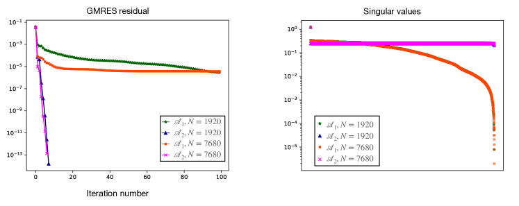
Figure 1: The singular values of the matrices for $\mathcal{A}_{1}$, and $\mathcal{A}_{2}$, for a sphere discretized with fourth order patches, and $N=1920$, and $7680$ (left) and the GMRES residual as a function of iteration number (right).

The poorer performance of $\mathcal{A}_{1}$ in an iterative solver as compared to $\mathcal{A}_{2}$ can be attributed to the lack of numerical second-kindness in its implementation. A discretized numerical operator is defined to be numerically second-kind if the identity term of the discretized integral operator is handled explicitly as is the case for $\mathcal{A}_{2}$ and $\mathcal{A}_{3}$. Any numerical discretization of integral operators is inherently compact since the operator is approximated via a finite-rank operator. This results in the spectrum of the discretized integral operator clustering closely to the origin which can result in numerical conditioning issues. Explicitly adding the identity term, as is the case in $\mathcal{A}_{2}$, results in the spectrum of the discretized integral operator clustering at $-1/4$. This greatly enhances the convergence of iterative methods such as GMRES [37].

To avoid any additional errors due to using the FMM, we illustrate this behavior on a smaller problem which would allow for using dense linear algebra routines. Consider the Laplace-Beltrami operator on the sphere with data given by a random fourth-order spherical harmonic expansion,

$$f(\theta,\phi)=\text{Re}\left(\sum_{n=1}^{4}\sum_{m=0}^{n}c_{n,m}Y_{n,m}(\theta,\phi)\right)\,,$$ (6.4)

where $c_{n,m}$ as before are complex numbers with real and imaginary parts uniformly sampled in $(-0.5,0.5)$. We restrict our attention to $p=4$ and $N=1920$ or $7680$. The linear system is then solved using GMRES with $\varepsilon_{\textrm{GMRES}}=10^{-14}$, and $\varepsilon=5\times 10^{-8}$. The matrices corresponding to the integral equations are precomputed and at every iteration the matrix vector product is computed using BLAS routines. Referring to Figure 1, we see that the GMRES residual for $\mathcal{A}_{2}$ drops exponentially with iteration number, while that for $\mathcal{A}_{1}$ converges at a slower rate and eventually stalls. The plot of the singular values for the two operators validates the lack of numerical second-kindness of $\mathcal{A}_{1}$ as well as the stability of condition number under refinement for the numerically second-kind $\mathcal{A}_{2}$. Finally, note that the smallest singular value for $\mathcal{A}_{1}$ decreases approximately by a factor of $4$ upon refinement, indicating that it might be proportional to area of the triangulated patches.

6.3 Harmonic fields

In this section, we present the numerical results for the computation of the harmonic vector fields on two geometries: a twisted torus geometry whose boundary $\Gamma$ is parametrized by $\bm{X}:[0,2\pi]^{2}\to\Gamma$ with

$$\bm{X}(u,v)=\sum_{i=-1}^{2}\sum_{j=-1}^{2}\delta_{i,j}\begin{pmatrix}\cos{v}\cos{((1-i)u+jv)}\\ \sin{v}\cos{((1-i)u+jv)}\\ \sin{((1-i)u+jv)}\\ \end{pmatrix}\,,$$ (6.5)

where the non-zero coefficients are

$$\delta_{-1,-1} =0.17, \qquad\delta_{-1,0} =0.11, \qquad\delta_{0,0} =1,$$ (6.6)

$$\delta_{1,0} =4.5, \delta_{2,0} =-0.25, \delta_{0,1} =0.01,$$

$$\delta_{2,1} =-0.45,$$

and a genus-10 surface obtained by first constructing the surface as a union of rectangular faces. A high-order mesh for a smooth version of the geometry is obtained using the surface smoother algorithm of [40], see LABEL:fig:g10 for a graphical depiction. For both examples, the surface is discretized with order $p=9$ patches. The quadrature and GMRES tolerances were set to $\varepsilon=5\times 10^{-8}$, and $\varepsilon_{\textrm{GMRES}}=5\times 10^{-10}$, respectively. In a slight abuse of notation, let $t_{s}$ now denote the time taken for computing the Hodge decomposition of a given vector field, which corresponds to solving two Laplace-Beltrami problems. Since the computation of the quadrature corrections tend to be the dominant cost, we reuse the computed quadrature corrections across the two solves. The solution to the Laplace-Beltrami problems were computed using the representation $\mathcal{A}_{3}$.

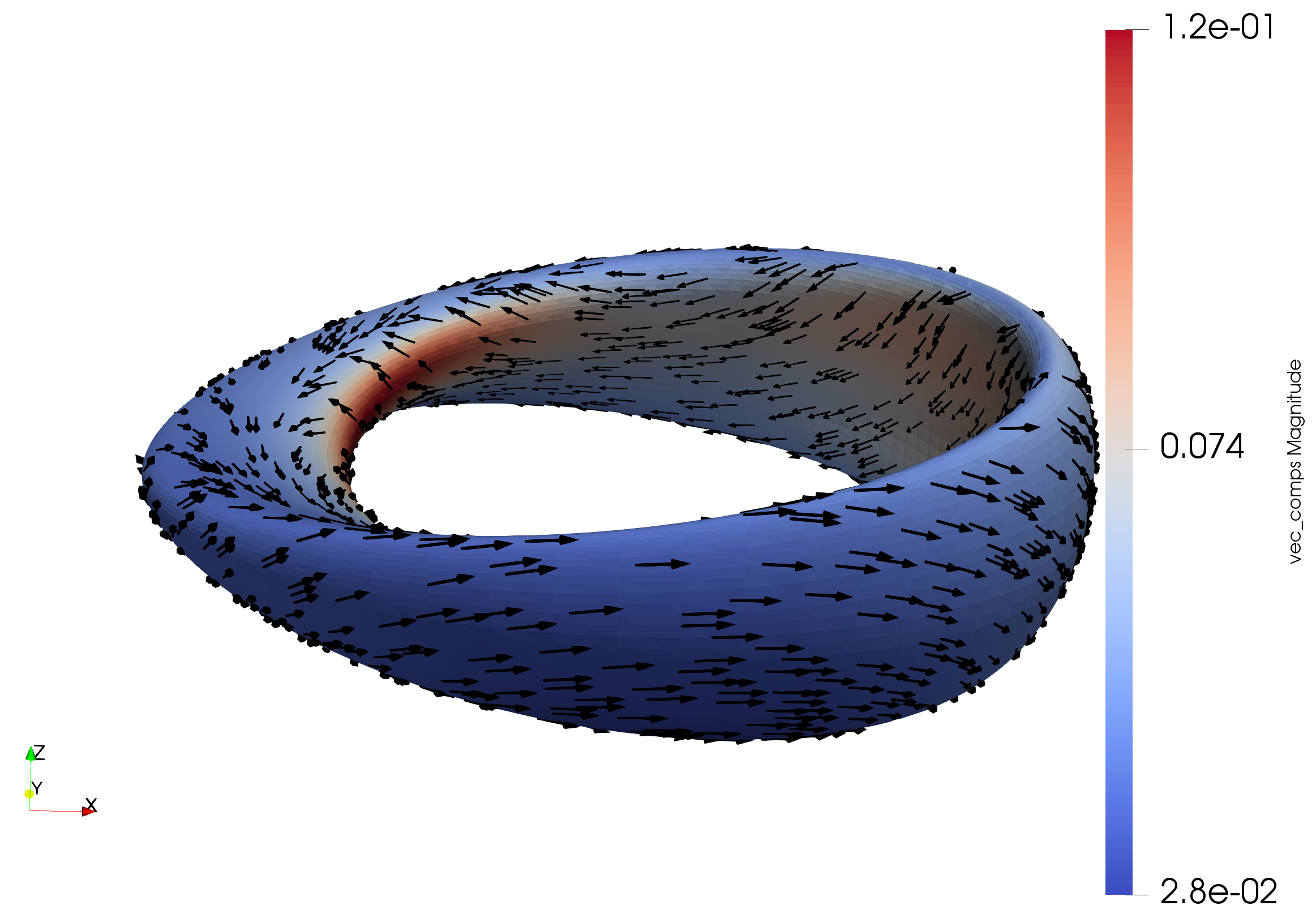
(a) Tangential vector field, $\mathbf{F}$

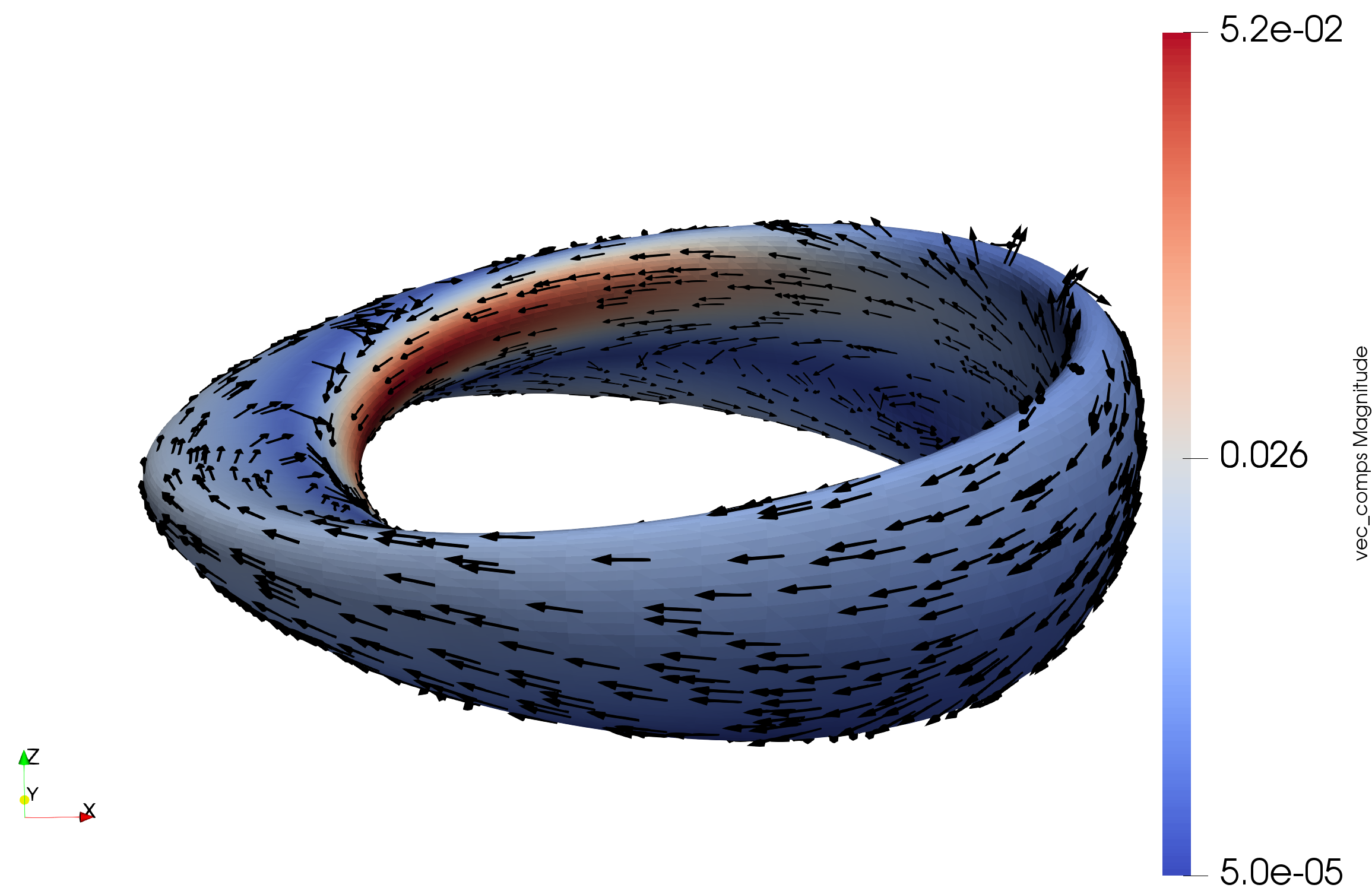
(b) Curl-free component, $\nabla_{\Gamma}\alpha$

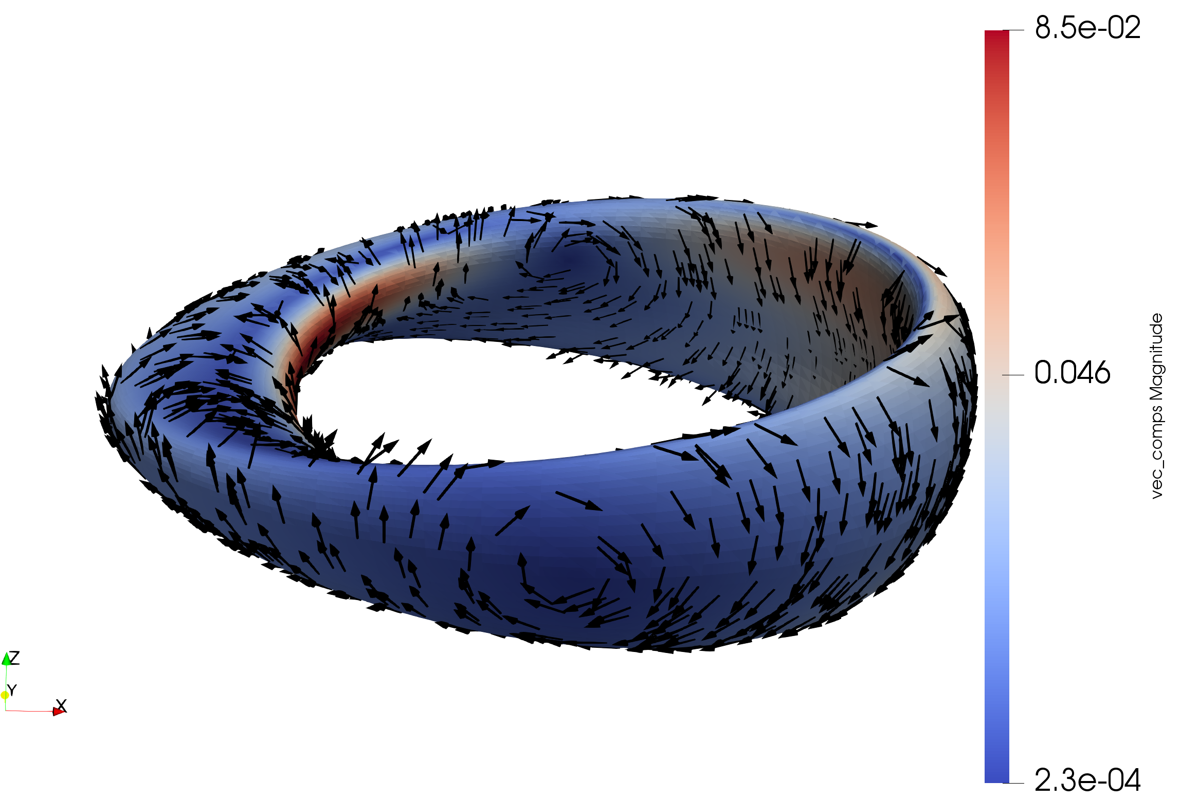
(c) Div-free component, $\mathbf{n}\times\nabla_{\Gamma}\beta$

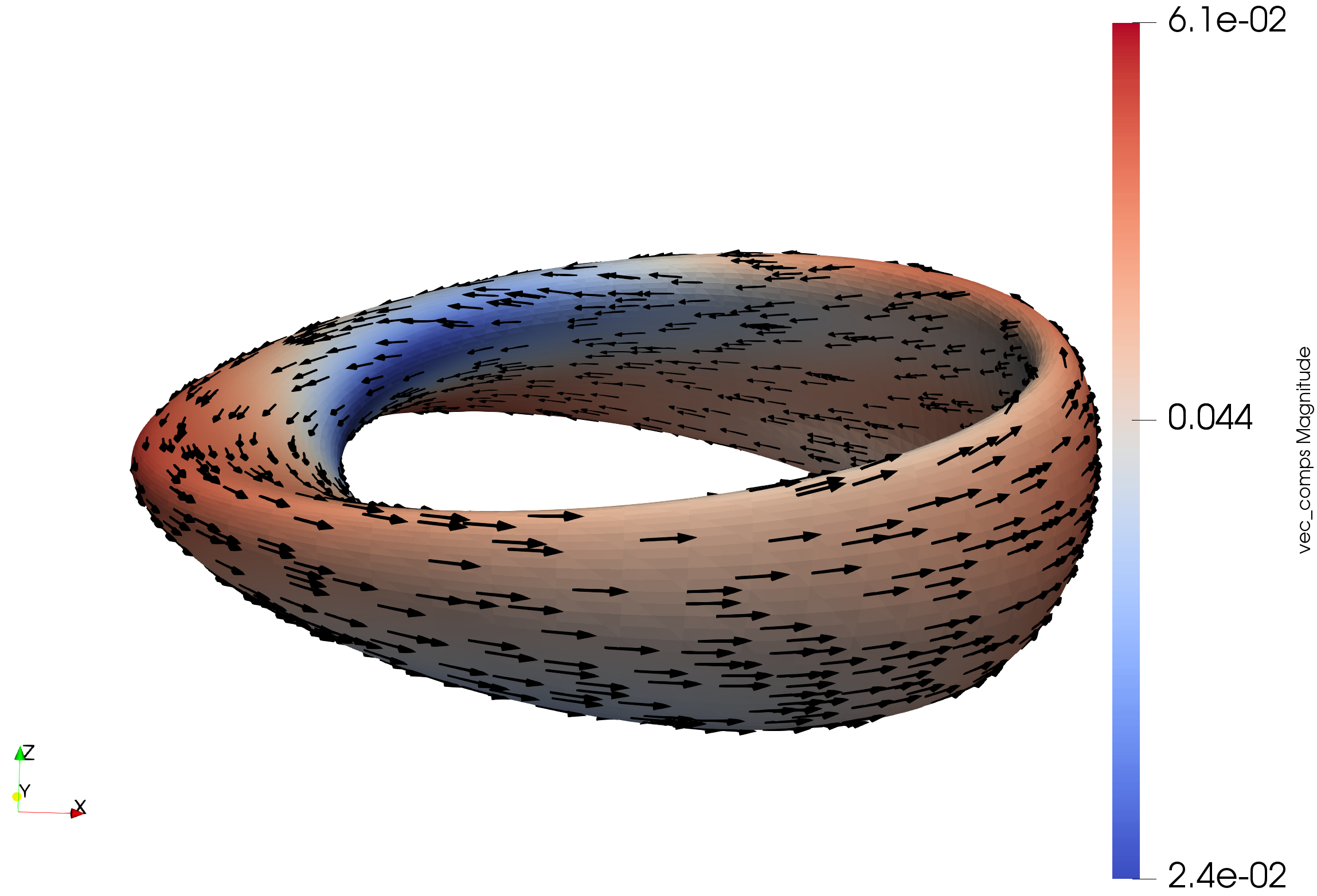
(d) Harmonic component, $\mathbf{H}$

Figure 2: Hodge decomposition on a twisted torus with initial field $\bm{V}$ given by a point current source at $\bm{x}_{0}$. The color bar represents the magnitude of the vector field and the arrows represent the direction of the field.

$p$	$N$	$n_{\textrm{iter}}$	$t_{s}$	$||\nabla_{\Gamma}\cdot\mathbf{\bm{H}}||_{\mathbb{L}^{2}(\Gamma)}$	$||\nabla_{\Gamma}\cdot(\mathbf{n}\times\mathbf{\bm{H}})||_{\mathbb{L}^{2}(\Gamma)}$
9	27,000	(27,28)	317.1	$1.4\times 10^{-2}$	$1.0\times 10^{-2}$
9	108,000	(27,28)	1182.0	$2.8\times 10^{-4}$	$1.5\times 10^{-4}$

Table 3: Results summary for computing harmonic vector fields on the twisted torus geometry.

For the twisted torus example, let $\bm{V}=\bm{\ell}\times(\bm{x}-\bm{x}_{0})/|\bm{x}-\bm{x}_{0}|^{3}$, with $\bm{x}_{0}=(0.2,0.2,0.2)$ and $\bm{\ell}=(0,1,1)$, and then define $\bm{F}=-\bm{n}\times\bm{n}\times\bm{V}$. It is straightforward to see that a current source defined in the exterior projects onto the harmonic vector fields for the torus. In Figure 2, we plot the tangential vector field $\bm{F}$, its curl-free component, its divergence-free component and the harmonic vector field $\bm{H}$. The second linearly independent harmonic vector field can be obtained by computing $\bm{n}\times\bm{H}$. In Table 3, we tabulate the number of iterations for computing the curl-free and divergence-free parts of decomposition denoted by $n_{\textrm{iter}}$, and the solve time $t_{s}$. The error in the computation of the harmonic vector fields is estimated by computing the $\mathbb{L}^{2}$ norm of $\nabla_{\Gamma}\cdot\bm{H}$ and $\nabla_{\Gamma}\cdot(\bm{n}\times\bm{H})$ using spectral differentiation. For this example $\|\bm{H}\|\approx 0.62498$, so the above error estimate serves as a proxy for the relative error as well.

We also compute the 20 linearly independent harmonic vector fields on a genus 10 surface. For this geometry, we choose a random surface vector field $\bm{V}$ whose components are random tensor product Legendre polynomials as discussed in Section 5. In LABEL:fig:g10, we plot the surface along with these 20 linearly independent harmonic vector fields computed using our solver. As before, we verify the computations by calculating the $\mathbb{L}^{2}$ norms of the surface divergence of $\bm{H}$ and $\bm{n}\times\bm{H}$, where $\bm{H}$ is the computed harmonic field. In Table 4, we tabulate the number of iterations for computing the curl-free and divergence-free parts of decomposition for one of the solves on the genus 10 surface, and also the computation time for obtaining the hodge decomposition.

Table 4: Results summary for computing harmonic vector fields on the genus 10 geometry.

$p$	$N$	$n_{\textrm{iter}}$	$t_{s}$	$||\nabla_{\Gamma}\cdot\mathbf{H}||_{\mathbb{L}^{2}(\Gamma)}$	$||\nabla_{\Gamma}\cdot\mathbf{n}\times\mathbf{H}||_{\mathbb{L}^{2}(\Gamma)}$
9	388,800	(19,19)	2910.5	$3.2\times 10^{-2}$	$5.6\times 10^{-3}$
9	1,555,200	(19,18)	10298.0	$5.8\times 10^{-4}$	$6.5\times 10^{-5}$

The summarized results for both examples illustrate the linear scaling of the algorithm, and also the constancy of number of GMRES iterations under mesh refinement.

7 Conclusions and future work

In this paper, we have presented a high-order FMM-accelerated iterative solver for the numerical solution of the Laplace-Beltrami equation on complex smooth surfaces in three dimensions. The Laplace-Beltrami problem $\Delta_{\Gamma}\psi=f$ is converted to a second-kind integral equation by representing the solution as $\psi=\mathcal{S}[\sigma]$ or $\psi=\mathcal{S}^{2}[\sigma]$, and using appropriate Caldéron identities. The resulting integral equation, which requires the application of various Laplace layer potentials, is then discretized using a high-order method with locally corrected quadratures for computing the weakly-singular layer potentials; their application is accelerated using fast multipole methods.

While the integral equation can be written in several equivalent analytic forms, we demonstrate the necessity of maintaining numerical second-kindness by explicitly isolating the identity term of the Fredholm equation in order to avoid stagnation of iterative solvers such as GMRES. We also illustrate that the using the representation $\psi=\mathcal{S}^{2}[\sigma]$ has the better numerical performance over using $\psi=\mathcal{S}[\sigma]$ and preconditioning with $\mathcal{S}$.

Finally, we also presented numerical examples demonstrating the computation of harmonic vector fields on surfaces using the Laplace-Beltrami solver. These vector fields are both of pure mathematical interest and are also required for solving problems in type I superconductivity and electromagnetism on topologically non-trivial geometries.

There are still several open questions that remain to be addressed. These include coupling high-order discretizations of the Laplace-Beltrami integral equations to fast direct solvers; subsequently using these solvers to develop iterative solvers for the solution of Maxwell’s equations using the generalized Debye formulation; and extending these ideas for the solution of surface diffusion problems that arise in pattern formation and cell biology. These are all ongoing areas of research.

8 Data availability

The code used in the numerical examples in this manuscript is available in two publicly accessible git repositories:

• https://github.com/flatironinstitute/FMM3D

• https://github.com/fastalgorithms/fmm3dbie

9 Funding

Dhwanit Agarwal’s research was supported in part by UT-Austin CoLab and UTEN Partnership, and the Portuguese Science and Technology Foundation under funding  #201801976/UTA18-001217. Michael O’Neil’s research was supported in part by the Office of Naval Research under award numbers #N00014-17-1-2451 and #N00014-18-1-2307, and the Simons Foundation/SFARI (560651, AB).

10 Conflict of interest

The authors do not have any conflicts of interest.

References

- [1] K. E. Atkinson and D. Chien. Piecewise polynomial collocation for boundary integral equations. SIAM J. Scientific Computing, 16:651–681, 1995.
- [2] E. Bänsch, P. Morin, and R. H. Nochetto. A finite element method for surface diffusion: the parametric case. J. Comput. Phys., 203(1):321–343, 2005.
- [3] L. Beirão da Veiga, F. Brezzi, L. D. Marini, and A. Russo. The hitchhiker’s guide to the virtual element method. Math. Models Meth. in Appl. Sci., 24(08):1541–1573, 2014.
- [4] M. Bertalmıo, L.-T. Cheng, S. Osher, and G. Sapiro. Variational problems and partial differential equations on implicit surfaces. J. Comput. Phys., 174(2):759–780, 2001.
- [5] A. Bonito, A. Demlow, and R. H. Nochetto. Finite element methods for the Laplace–Beltrami operator. In Handbook of Numerical Analysis, volume 21, pages 1–103. Elsevier, 2020.
- [6] J. Bremer. On the Nyström discretization of integral equations on planar curves with corners. Appl. Comput. Harm. Anal., 32:45–64, 2012.
- [7] E. Burman, P. Hansbo, M. G. Larson, and A. Massing. A cut discontinuous Galerkin method for the Laplace–Beltrami operator. IMA J. Num. Anal., 37(1):138–169, 2017.
- [8] Y. Chen and C. B. Macdonald. The closest point method and multigrid solvers for elliptic equations on surfaces. SIAM J. Sci. Comput., 37(1):A134–A155, 2015.
- [9] Q. I. Dai, W. C. Chew, L. J. Jiang, and Y. Wu. Differential-Forms-Motivated Discretizations of Electromagnetic Differential and Integral Equations. IEEE Ant. Wire. Propag. Lett., 13:1223–1226, 2014.
- [10] A. Demlow and G. Dziuk. An adaptive finite element method for the Laplace–Beltrami operator on implicitly defined surfaces. SIAM J. Num. Anal., 45(1):421–442, 2007.
- [11] C. Epstein and L. Greengard. Debye sources and the numerical solution of the time harmonic Maxwell equations. Comm. Pure Appl. Math, 63(4):413–463, 2010.
- [12] C. L. Epstein, Z. Gimbutas, L. Greengard, A. Klöckner, and M. O’Neil. A consistency condition for the vector potential in multiply-connected domains. IEEE Trans. Magn., 49(3):1072–1076, 2013.
- [13] C. L. Epstein, L. Greengard, and M. O’Neil. Debye sources and the numerical solution of the time harmonic Maxwell equations II. Comm. Pure Appl. Math., 66(5):753–789, 2013.
- [14] C. L. Epstein and M. Rachh. Debye source representation for type-I superconductors, I. J. Comput. Phys., 452:110892, 2022.
- [15] T. Frankel. The Geometry of Physics. Cambridge University Press, New York, NY, 2011.
- [16] M. Frittelli and I. Sgura. Virtual element method for the Laplace-Beltrami equation on surfaces. ESAIM: Mathematical Modelling and Numerical Analysis, 52(3):965–993, 2018.
- [17] T. Goodwill and M. O’Neil. An interface formulation of the Laplace-Beltrami problem on piecewise smooth surfaces. arXiv:2108.08959, 2022.
- [18] L. Greengard, M. O’Neil, M. Rachh, and F. Vico. Fast multipole methods for the evaluation of layer potentials with locally-corrected quadratures. J. Comput. Phys.: X, 10:100092, 2021.
- [19] L. Greengard and V. Rokhlin. A new version of the Fast Multipole Method for the Laplace equation in three dimensions. Acta Numerica, 6:229–269, 1997.
- [20] J. B. Greer, A. L. Bertozzi, and G. Sapiro. Fourth order partial differential equations on general geometries. J. Comput. Phys., 216(1):216–246, 2006.
- [21] L.-M. Imbert-Gerard and L. Greengard. Pseudo-Spectral Methods for the Laplace-Beltrami equation and the Hodge decomposition on Surfaces of Genus One. Numer. Methods Partial. Differ. Equ., 33(3):941–955, 2017.
- [22] J. Jost. Riemannian geometry and geometric analysis. Springer Verlag, 2011.
- [23] H. Kim, A. Yun, S. Yoon, C. Lee, J. Park, and J. Kim. Pattern formation in reaction–diffusion systems on evolving surfaces. Comput. Math. with Appl., 80(9):2019–2028, 2020.
- [24] T. Koornwinder. Two-variable analogues of the classical orthogonal polynomials. In Theory and application of special functions (Proc. Advanced Sem., Math. Res. Center, Univ. Wisconsin, Madison, Wis., 1975), pages 435–495. Academic Press New York, 1975.
- [25] R. Kress. Linear Integral Equations. Springer, New York, NY, 2014.
- [26] J. Kromer and D. Bothe. Highly accurate numerical computation of implicitly defined volumes using the Laplace-Beltrami operator. arXiv:1805.03136, 2018.
- [27] M. C. A. Kropinski and N. Nigam. Fast integral equation methods for the Laplace-Beltrami equation on the sphere. Adv. Comput. Math., 40(2):577–596, 2014.
- [28] M. C. A. Kropinski, N. Nigam, and B. Quaife. Integral equation methods for the Yukawa-Beltrami equation on the sphere. Adv. Comput. Math., 42(2):469–488, 2016.
- [29] C. B. Macdonald and S. J. Ruuth. Level set equations on surfaces via the closest point method. J. Sci. Comput., 35(2):219–240, 2008.
- [30] C. B. Macdonald and S. J. Ruuth. The implicit closest point method for the numerical solution of partial differential equations on surfaces. SIAM J. Sci. Comput., 31(6):4330–4350, 2010.
- [31] D. Malhotra, A. Cerfon, L.-M. Imbert-Gérard, and M. O’Neil. Taylor states in stellarators: A fast high-order boundary integral solver. J. Comput. Phys., 397:108791, 2019.
- [32] J. Nedelec. Acoustic and Electromagnetic Equations. Springer, New York, NY, 2001.
- [33] M. O’Neil. Second-kind integral equations for the Laplace-Beltrami problem on surfaces in three dimensions. Adv. Comput. Math., 44(5):1385–1409, 2018.
- [34] R. G. Plaza, F. Sanchez-Garduno, P. Padilla, R. A. Barrio, and P. K. Maini. The effect of growth and curvature on pattern formation. J. Dynamics Diff. Equations, 16(4):1093–1121, 2004.
- [35] A. Rahimian, I. Lashuk, S. Veerapaneni, A. Chandramowlishwaran, D. Malhotra, L. Moon, R. Sampath, A. Shringarpure, J. Vetter, R. Vuduc, et al. Petascale direct numerical simulation of blood flow on 200k cores and heterogeneous architectures. In SC’10: Proceedings of the 2010 ACM/IEEE International Conference for High Performance Computing, Networking, Storage and Analysis, pages 1–11. IEEE, 2010.
- [36] S. Rosenberg. The Laplacian on a Riemannian Manifold. Cambridge University Press, 1997.
- [37] Y. Saad and M. H. Schultz. GMRES: A Generalized Minimal Residual Algorithm for Solving Nonsymmetric Linear Systems. SIAM J. Sci. Stat. Comput., 7:856–869, 1986.
- [38] J. Sifuentes, Z. Gimbutas, and L. Greengard. Randomized methods for rank-deficient linear systems. Elec. Trans. Num. Anal., 44:177–188, 2015.
- [39] S. K. Veerapaneni, A. Rahimian, G. Biros, and D. Zorin. A fast algorithm for simulating vesicle flows in three dimensions. J. Comput. Phys., 230:5610–5634, 2011.
- [40] F. Vico, L. Greengard, M. O’Neil, and M. Rachh. A fast boundary integral method for high-order multiscale mesh generation. SIAM J. Sci. Comput., 42(2):A1380–A1401, 2020.
- [41] B. Vioreanu and V. Rokhlin. Spectra of Multiplication Operators as a Numerical Tool. SIAM J. Sci. Comput., 36:A267–A288, 2014.
- [42] M. Wang, S. Leung, and H. Zhao. Modified Virtual Grid Difference for Discretizing the Laplace–Beltrami Operator on Point Clouds. SIAM J. Sci. Comput., 40(1):A1–A21, 2018.