On the DLM/FD methods for simulating neutrally buoyant swimmer motion in non-Newtonian shear thinning fluids

Ang Li^a, Tsorng-Whay Pan^b,, and Roland Glowinski^{b a} Department of Mathematics, Lane College, Jackson, Tennessee 38301, USA ^b Department of Mathematics, University of Houston, Houston, Texas 77204, USA

Abstract In this article we discuss the generalization of a Lagrange multiplier based fictitious domain (DLM/FD) method to simulating the motion of neutrally buoyant particles of non-symmetric shape in non-Newtonian shear thinning fluids. Numerical solutions of steady Poiseuille flow of non-Newtonian shear thinning fluids are compared with the exact solutions in a two-dimensional channel. Concerning a self-propelled swimmer formed by two disks, the effect of shear thinning makes the swimmer moving faster and decreases the critical Reynolds number (for the moving direction changing to the opposite one) when decreasing the value of the power index in the Carreau-Bird model.

keywords: Carreau-Bird model; Neutrally buoyant particle; Self-propelled swimmer; Fictitious domain method; Operator splitting; Finite element approximations.

1 Introduction

Micro-swimmers, like microorganisms, swimming in a low Reynolds number regime, encounter stringent constraints due to the dominance of viscous over inertial forces [1, 2]. As a result of kinetic reversibility, Purcell’s scallop theorem [1] rules out reciprocal motion (i.e., strokes with time-reversal symmetry) for effective locomotion in the absence of inertia in Newtonian fluids. Another important fact is that many biological fluids, including blood, respiratory and cervical mucus, have non-Newtonian properties, such as viscoelasticity and shear-thinning viscosity (i.e., the viscosity decreases non-linearly with the shear rate [3] and [4]). The physics governing microorganism locomotion at low Reynolds numbers in Newtonian fluids is relatively well understood, while low Reynolds propulsion in non-Newtonian fluids remains largely unexplored [2]. Since the scallop theorem does not hold in non-Newtonian fluids (see, e.g., [5] and [6]), it should be possible to design and build novel micro-swimmers that can move with reciprocal motion in non-Newtonian fluids. A study on a reciprocal sliding sphere swimmer in a shear-thinning (non-elastic) fluid [7] suggests that propulsion is achievable by reciprocal motion, in which backward and forward strokes occur at different rates. Similarly, another recent study in [8] reported that a symmetric micro-scallop, a single-hinge microswimmer, can propel in shear thickening and shear thinning (non-elastic) fluids at low Reynolds number. Thus reciprocal swimming mechanism can help in designing biomedical microdevices that can propel by a simple actuation scheme in biological fluids.

In this article, we have focused on the effect of shear thinning on the swimmer motion in a two-dimensional channel. To study such effect by direct numerical simulation, we have adapted the Carreau-Bird viscosity model (see [3] and [4]) for shear thinning property. For example, in [11] and [12], particle settling in Oldroyd-B viscoelastic fluids with shear thinning property was studied numerically by using the Carreau-Bird viscosity model. Direct simulation of the motion of particles has been carried out by using an arbitrary Lagrangian-Eulerian moving mesh technique with finite element method. The power law, which is the other commonly used model, was used to investigate the effects of both shear thickening and thinning on the motion of scallop swimmers numerically in [8]. A finite element method with the dynamic mesh-adaptation for moving boundaries was used to study how the scallop swimmer can swim by reciprocal motion at low (not zero) Reynolds number. For simulating the swimmer motion in non-Newtonian shear thinning fluids, we have extended a Lagrange multiplier based fictitious domain (DLM/FD) method developed for disks in [14] to simulate the motion of a neutrally buoyant non-symmetric swimmer in non-Newtonian shear thinning fluids. This non-symmetric swimmer of two disks with different radii is formed by connecting their mass centers with a massless spring like the one in, e.g., [9] and [10]. To keep the main flavor of the fictitious domain methods, i.e., the usage of fast solvers to solve the resulting linear systems, we have splitted the diffusion term in our proposed methodologies. Accurate computational solutions are obtained by the proposed methods for Poiseuille flow of non-Newtonian shear thinning fluids in a two-dimensional channel (thanks to the recently published exact solutions for such Poiseuille flow by Griffiths in [13]). Then we have further validated our proposed numerical methods by studying the migration of 56 disks in a two-dimensional channel, which was considered in [29]. For the effect of shear thinning on the swimmer motion, we have obtained that, via direct numerical simulation, the swimmer moves faster and the critical Reynolds number (for the moving direction changing to the opposite one) decreases when decreasing the value of the power index in the Carreau-Bird model. The content of this article is as follows: In Section 2 we introduce a fictitious domain formulation of the model problem associated with the neutrally buoyant particle cases; then in Section 3 we discuss the time and space discretizations and the related numerical methodology. We then present and discuss the numerical results in Section 4. Concluding remarks are given in Section 5.

2 A fictitious domain formulation of the model problem

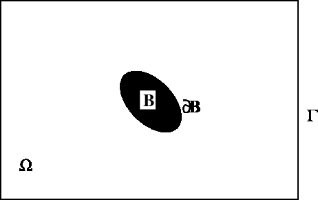
Figure 1: An example of two-dimensional flow region with one rigid body.

In [14], Pan and Glowinski developed a distributed Lagrange multiplier/fictitious domain (DLM/FD) method to simulate the motion of neutrally buoyant disks freely moving in a Newtonian viscous incompressible fluid in a two dimensional channel. Later they extended in [15], [16], and [17] such DLM/FD method to simulate and investigate the motion of neutrally buoyant balls in circular Poiseuille flows. In this article, we have extended the above DLM/FD method to study the motion of a self-propelled swimmer in non-Newtonian shear thinning fluids. This non-symmetric swimmer of two disks with different radii is formed by connecting their mass centers with a massless spring as the one in, e.g., [9] and [10]. In this section, we will address the DLM/FD formulation for such problem. Let $\Omega\subset{\text{I\!R}}^{2}$ be a rectangular region. We suppose that $\Omega$ is filled with a non-Newtonian viscous incompressible fluid of density $\rho_{f}$ and contains a moving neutrally buoyant rigid particle $B$ centered at ${\bf G}=\{G_{1},G_{2}\}^{T}$ of density $\rho_{f}$ as shown in Figure 1; the flow is modeled by the Navier-Stokes equations and the motion of $B$ is described by the Euler-Newton’s equations. Following the DLM/FD formulation developed in [14], we define

$$W_{0,p}=\{{\bf v}|{\bf v}\in(H^{1}(\Omega))^{2},\ {\bf v}={\bf 0}\ \text{\it on the top and bottom boundary of $\Omega$ and}$$

$$\hskip 55.0pt{\bf v}\ \text{\it is periodic in the $x_{1}$ direction}\},$$

$$L_{0}^{2}=\{q|q\in L^{2}(\Omega),\int_{\Omega}q\,d{\bf x}=0,\},$$

$$\Lambda_{0}(t)=\{{\boldsymbol{\mu}}|{\boldsymbol{\mu}}\in(H^{1}(B(t)))^{2},<{\boldsymbol{\mu}},{\bf e}_{i}>_{B(t)}=0,\ i=1,2,<{\boldsymbol{\mu}},{{\overrightarrow{Gx}}^{\perp}}>_{B(t)}=0\}$$

with ${\bf e}_{1}=\{1,0\}^{T}$, ${\bf e}_{2}=\{0,1\}^{T}$, ${{\overrightarrow{Gx}}^{\perp}}=\{-(x_{2}-G_{2}),x_{1}-G_{1}\}^{T}$ and $<\cdot,\cdot>_{B(t)}$ an inner product on $\Lambda_{0}(t)$ which can be the standard inner product on $(H^{1}(B(t)))^{2}$ (see [23], Section 5, for further information on the choice of $<\cdot,\cdot>_{B(t)}$). Then the fictitious domain formulation with distributed Lagrange multipliers for flow around a freely moving neutrally buoyant particle is as follows

$$For\ a.e.\ t>0,\ find\ {\bf u}(t)\in W_{0,p},\ p(t)\in L_{0}^{2},\ {\bf V}_{{\bf G}}(t)\in{\text{I\!R}}^{2},\ {\bf G}(t)\in{\text{I\!R}}^{2},$$

$$\omega(t)\in{\text{I\!R}},\ {\boldsymbol{\lambda}}(t)\in\Lambda_{0}(t)\ \ \text{\it such that}$$

(1) $$\begin{cases}\rho_{f}{\displaystyle{\int_{\Omega}}}\left[\dfrac{\partial{\bf u}}{\partial t}+({\bf u}\cdot{\boldsymbol{\nabla}}){\bf u}\right]\cdot{\bf v}\ d{\bf x}+2{\displaystyle{\int_{\Omega}}}\eta\ {\bf D}({\bf u})\boldsymbol{:}{\bf D}({\bf v})\ d{\bf x}-{\displaystyle{\int_{\Omega}}}p{\boldsymbol{\nabla}}\cdot{\bf v}\,d{\bf x}\\ \ \ \ -<{\boldsymbol{\lambda}},{\bf v}>_{B(t)}=\rho_{f}{\displaystyle{\int_{\Omega}}}{\bf g}\cdot{\bf v}\,d{\bf x}+{\displaystyle{\int_{\Omega}}}{\bf F}\cdot{\bf v}\,d{\bf x},\ \forall{\bf v}\in W_{0,p},\end{cases}$$

(2) $${\displaystyle{\int_{\Omega}}}q{\boldsymbol{\nabla}}\cdot{\bf u}(t)d{\bf x}=0,\ \forall q\in L^{2}(\Omega),$$

(3) $$<{\boldsymbol{\mu}},{\bf u}(t)>_{B(t)}=<{\boldsymbol{\mu}},{\bf u}_{p}(t)>_{B(t)},\ \forall{\boldsymbol{\mu}}\in\Lambda_{0}(t),$$

(4) $$\dfrac{d{\bf G}}{dt}={\bf V}_{{\bf G}},$$

(5) $${\bf V}_{{\bf G}}(0)={\bf V}_{{\bf G}}^{0},\ \omega(0)=\omega^{0},\ {\bf G}(0)={\bf G}^{0}=\{G^{0}_{1},G^{0}_{2}\}^{T},$$

(6) $${\bf u}({\bf x},0)={\overline{\bf u}}_{0}({\bf x})=\begin{cases}{\bf u}_{0}({\bf x}),\ \forall{\bf x}\in{\Omega\backslash\overline{B(0)}},\\ {\bf V}_{{\bf G}}^{0}+\omega^{0}\{-(x_{2}-G^{0}_{2}),x_{1}-G^{0}_{1}\}^{T},\ \forall{\bf x}\in\overline{B(0)},\end{cases}$$

where ${\bf u}$ and $p$ denote velocity and pressure, respectively, $\eta(\dot{\gamma})$ is the fluid viscosity, ${\boldsymbol{\lambda}}$ is a Lagrange multiplier, ${\bf D}({\bf v})=({\boldsymbol{\nabla}}{\bf v}+{\boldsymbol{\nabla}}{\bf v}^{T})/2$, ${\bf g}$ is gravity, ${\bf F}$ is the pressure gradient pointing in the $x_{1}$ direction for particle moving in a Poiseuille flow, ${\bf V}_{{\bf G}}$ is the translation velocity of the particle $B$, and $\omega$ is the angular velocity of $B$. We suppose that the no-slip condition holds on $\partial B$. We also use, if necessary, the notation $\phi(t)$ for the function ${\bf x}\to\phi({\bf x},t)$. In equation (3), ${\bf u}_{p}(t)$ is a part of actual particle motion given as follows

$${\bf u}({\bf x},t)={\bf V}_{{\bf G}}(t)+\omega(t)\{-(x_{2}-G_{2}),x_{1}-G_{1}\}^{T}+{\bf u}_{p}({\bf x},t).$$

Thus we have ${\bf u}_{p}={\bf 0}$ if $B$ is a single piece neutrally buoyant rigid particle like a disk suspended in fluid; but for $B$ as a swimmer formed by two neutrally buoyant disks considered in this article, ${\bf u}_{p}(t)$ is a given reciprocal motion of the two disks with respect to the swimmer mass center (see Section 4). Shear thinning can be easily added to the above model by using the Carreau-Bird viscosity model (see, [3] and [4])

(7) $$\dfrac{\eta-\eta_{\infty}}{\eta_{0}-\eta_{\infty}}=(1+(\lambda_{3}\dot{\gamma})^{2})^{(n-1)/2},$$

where $\eta_{0}$ (resp., $\eta_{\infty}$) is the fluid viscosity at zero shear rate (resp., infinite shear rate), $\lambda_{3}$ is the relaxation time, $\dot{\gamma}$ is determined by the second invariant of the rate of strain tensor $(\dot{\gamma})^{2}=({\bf D}({\bf u}):{\bf D}({\bf u}))/2$, and the power index $n$ is in $(0,1]$ (if $n=1$, the fluid is a Newtonian fluid with constant viscosity $\eta_{0}$).

Remark 1.

In (3), the rigid body motion in the region occupied by the particle is enforced via Lagrange multipliers ${\boldsymbol{\lambda}}$. To recover the translation velocity ${\bf V}_{{\bf G}}(t)$ and the angular velocity $\omega(t)$, we solve the following equations

(8) $$\begin{cases}<{\bf e}_{i},{\bf u}(t)-{\bf V}_{{\bf G}}(t)-\omega(t)\ {{\overrightarrow{Gx}}^{\perp}}>_{B(t)}=0,\ for\ i=1,2,\\ <{{\overrightarrow{Gx}}^{\perp}},{\bf u}(t)-{\bf V}_{{\bf G}}(t)-\omega(t)\ {{\overrightarrow{Gx}}^{\perp}}>_{B(t)}=0.\end{cases}$$

3 Space approximation and time discretization

Concerning the finite element based space approximation of problem (1)-(6), we use $P_{1}$-$iso$-$P_{2}$ and $P_{1}$ finite elements for the velocity field and pressure, respectively (see, e.g., [18] and [19](Chapter 5)). More precisely with $h$ a space discretization step, we introduce a finite element triangulation ${\mathcal{T}_{h}}$ of ${\overline{\Omega}}$ and then ${\mathcal{T}}_{2h}$ a triangulation twice coarser. Then we approximate $W_{0,p}$, $L^{2}$ and $L^{2}_{0}$ by the following finite dimensional spaces

(9) $$W_{0,h}=\{{\bf v}_{h}|{\bf v}_{h}\in(C^{0}(\overline{\Omega}))^{2},\ {\bf v}_{h}|_{T}\in P_{1}\times P_{1},\ \forall T\in{\mathcal{T}}_{h},\ {\bf v}_{h}={\bf 0}\ \text{\it on the}$$

$$\hskip 60.0pt\text{\it top and bottom boundary of $\Omega$ and}\ {\bf v}\ \text{\it is periodic in the $x_{1}$ direction}\ \},$$

$$L^{2}_{h}=\{q_{h} | q_{h}\in C^{0}(\overline{\Omega}),\ q_{h}|_{T}\in P_{1},\ \forall T\in{\mathcal{T}}_{2h},\ q_{h}\ \text{\it is periodic}$$

$$\text{\it in the $x_{1}$ direction}\},$$

and

(11) $$L^{2}_{0,h}=\{q_{h}|q_{h}\in L^{2}_{h},\ \int_{\Omega}q_{h}\,d{\bf x}=0\},$$

respectively; in (9)-(11), $P_{1}$ is the space of polynomials in two variables of degree $\leq 1$.

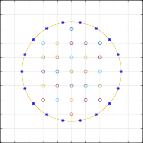
Figure 2: An example of set of collocation points chosen inside the disk and at its boundary for enforcing the rigid body motion.

A finite dimensional space approximating $\Lambda_{0}(t)$ is defined in the following: let $\{{\bf x}_{i}\}_{i=1}^{N}$ be a set of points covering $\overline{B(t)}$; we define then

(12) $$\Lambda_{h}(t)=\{{\boldsymbol{\mu}}_{h}|{\boldsymbol{\mu}}_{h}={\displaystyle\sum}_{i=1}^{N}{\boldsymbol{\mu}}_{i}\delta({\bf x}-{\bf x}_{i}),\ {\boldsymbol{\mu}}_{i}\in{\text{I\!R}}^{2},\ \forall i=1,...,N\},$$

where $\delta(\cdot)$ is the Dirac measure at ${\bf x}={\bf 0}.$ Then, instead of the inner product of $(H^{1}(B(t)))^{2}$ we shall use $<\cdot,\cdot>_{B_{h}(t)}$ defined by

(13) $$<{\boldsymbol{\mu}}_{h},{\bf v}_{h}>_{B_{h}(t)}={\displaystyle\sum}_{i=1}^{N}{\boldsymbol{\mu}}_{i}\cdot{\bf v}_{h}({\bf x}_{i}),\ \forall{\boldsymbol{\mu}}_{h}\in\Lambda_{h}(t),\ {\bf v}_{h}\in W_{0,h}.$$

Then we approximate $\Lambda_{0}(t)$ by

(14) $$\Lambda_{0,h}(t)=\{\mu_{h}|\mu_{h}\in\Lambda_{h}(t),\ <\mu_{h},{\bf e}_{i}>_{B_{h}(t)}=0,\ i=1,2,\ <\mu_{h},{{\overrightarrow{Gx}}^{\perp}}>_{B_{h}(t)}=0\}.$$

A typical choice of points for defining (12) is to take the grid points of the velocity mesh internal to the particle $B$ and whose distance to the boundary of $B$ is greater than, e.g. $h$, and to complete with selected points from the boundary of $B(t)$ (see Figure 2).

Using the above finite dimensional spaces leads to the following approximation of problem (1)-(6):

$$For\ a.e.\ t>0,\ find\ {\bf u}(t)\in W_{0,h},\ p(t)\in L_{0,h}^{2},\ {\bf V}_{{\bf G}}(t)\in{\text{I\!R}}^{2},\ {\bf G}(t)\in{\text{I\!R}}^{2},$$

$$\omega(t)\in{\text{I\!R}},\ {\boldsymbol{\lambda}}_{h}(t)\in\Lambda_{0,h}(t)\ \ \text{\it such that}$$

(15) $$\begin{cases}\rho_{f}{\displaystyle{\int_{\Omega}}}\left[\dfrac{\partial{\bf u}_{h}}{\partial t}+({\bf u}_{h}\cdot{\boldsymbol{\nabla}}){\bf u}_{h}\right]\cdot{\bf v}\,d{\bf x}+2{\displaystyle{\int_{\Omega}}}\eta\ {\bf D}({\bf u}_{h})\boldsymbol{:}{\bf D}({\bf v})\ d{\bf x}\\ \hskip 20.0pt-{\displaystyle{\int_{\Omega}}}p_{h}{\boldsymbol{\nabla}}\cdot{\bf v}\,d{\bf x}-<{\boldsymbol{\lambda}}_{h},{\bf v}>_{B_{h}(t)}={\displaystyle{\int_{\Omega}}}{\bf F}\cdot{\bf v}\,d{\bf x},\ \forall{\bf v}\in W_{0,h},\end{cases}$$

(16) $${\displaystyle{\int_{\Omega}}}q{\boldsymbol{\nabla}}\cdot{\bf u}_{h}(t)d{\bf x}=0,\ \forall q\in L^{2}_{h},$$

(17) $$<{\boldsymbol{\mu}},{\bf u}_{h}(t)>_{B_{h}(t)}=<{\boldsymbol{\mu}},{\bf u}_{p}(t)>_{B_{h}(t)},\ \forall{\boldsymbol{\mu}}\in\Lambda_{0,h}(t),$$

(18) $$\dfrac{d{\bf G}}{dt}={\bf V}_{{\bf G}},$$

(19) $${\bf V}_{{\bf G}}(0)={\bf V}_{{\bf G}}^{0},\ \omega(0)=\omega^{0},\ {\bf G}(0)={\bf G}^{0}=\{G^{0}_{1},G^{0}_{2}\}^{T},$$

(20) $${\bf u}_{h}({\bf x},0)={\overline{\bf u}}_{0,h}({\bf x})\ (\text{with}{\boldsymbol{\nabla}}\cdot{\overline{\bf u}}_{0,h}=0).$$

Applying a first order operator splitting scheme, namely the Lie scheme [20] (see also [19] and [21] (Chapter 2)), to discretize equations (15)-(20) in time, we obtain (after dropping some of the subscripts $h$):

(21) $${\bf u}^{0}={\overline{\bf u}}_{0,h},\ {\bf V}_{{\bf G}}^{0},\ \omega^{0},\ and\ {\bf G}^{0}\ are\ given;$$

For $n\geq 0$, knowing ${\bf u}^{n}$, ${\bf V}_{{\bf G}}^{n}$, $\omega^{n}$ and ${\bf G}^{n}$, compute ${\bf u}^{n+1/6}$ and $p^{n+1/6}$ via the solution of

(22) $$\begin{cases}\displaystyle\rho_{f}{\displaystyle{\int_{\Omega}}}\frac{{\bf u}^{n+1/6}-{\bf u}^{n}}{\triangle t}\cdot{\bf v}\,d{\bf x}-{\displaystyle{\int_{\Omega}}}p^{n+1/6}{\boldsymbol{\nabla}}\cdot{\bf v}\,d{\bf x}=0,\ \forall{\bf v}\in W_{0,h},\\ \displaystyle{\displaystyle{\int_{\Omega}}}q{\boldsymbol{\nabla}}\cdot{\bf u}^{n+1/6}\,d{\bf x}=0,\ \forall q\in L^{2}_{h};\ {\bf u}^{n+1/6}\in W_{0,h},\ p^{n+1/6}\in L^{2}_{0,h}.\end{cases}$$

Then compute ${\bf u}^{n+2/6}$ via the solution of

(23) $$\begin{cases}\displaystyle{\displaystyle{\int_{\Omega}}}\frac{\partial{\bf u}}{\partial t}\cdot{\bf v}\,d{\bf x}+{\displaystyle{\int_{\Omega}}}({\bf u}^{n+1/6}\cdot{\boldsymbol{\nabla}}){\bf u}\cdot{\bf v}\,d{\bf x}=0,\ \forall{\bf v}\in W_{0,h},\ on\ (t^{n},t^{n+1}),\\ \displaystyle\ {\bf u}(t^{n})={\bf u}^{n+1/6};\ \ {\bf u}(t)\in W_{0,h},\end{cases}$$

(24) $${\bf u}^{n+2/6}={\bf u}(t^{n+1}).$$

Next, compute ${\bf u}^{n+3/6}$ via the solution of

(25) $$\begin{cases}\displaystyle\rho_{f}{\displaystyle{\int_{\Omega}}}\frac{{\bf u}^{n+3/6}-{\bf u}^{n+2/6}}{\triangle t}\cdot{\bf v}\,d{\bf x}+2\alpha{\displaystyle{\int_{\Omega}}}\eta(\dot{{\bf u}^{n+2/6}})\ {\bf D}({\bf u}^{n+3/6})\boldsymbol{:}{\bf D}({\bf v})\ d{\bf x}\\ \hskip 20.0pt={\displaystyle{\int_{\Omega}}}{\bf F}\cdot{\bf v}\,d{\bf x},\forall{\bf v}\in W_{0,h};\ \ {\bf u}^{n+3/6}\in W_{0,h}.\end{cases}$$

Now predict the position and the translation velocity of the center of mass of the particles as follows: Take ${\bf V}_{{\bf G}}^{n+\frac{4}{6},0}={\bf V}_{{\bf G}}^{n}$ and ${\bf G}^{n+\frac{4}{6},0}={\bf G}^{n}$; then predict the new position of the particle via the following sub-cycling and predicting-correcting technique:

For $$k=1,\dots,N$$, compute

(26) $${\widehat{\bf V}_{{\bf G}}}^{n+\frac{4}{6},k}={\bf V}_{{\bf G}}^{n+\frac{4}{6},k-1}+{\bf F}^{r}({\bf G}^{n+\frac{4}{6},k-1}){\triangle t}/{2N},$$

(27) $${\widehat{\bf G}}^{n+\frac{4}{6},k}={\bf G}^{n+\frac{4}{6},k-1}+({\widehat{\bf V}_{{\bf G}}}^{n+\frac{4}{6},k}+{\bf V}_{{\bf G}}^{n+\frac{4}{6},k-1}){\triangle t}/{4N},$$

(28) $${\bf V}_{{\bf G}}^{n+\frac{4}{6},k}={\bf V}_{{\bf G}}^{n+\frac{4}{6},k-1}+({\bf F}^{r}({\widehat{\bf G}}^{n+\frac{4}{6},k})+{\bf F}^{r}({\bf G}^{n+\frac{4}{6},k-1})){\triangle t}/{4N},$$

(29) $${\bf G}^{n+\frac{4}{6},k}={\bf G}^{n+\frac{4}{6},k-1}+({\bf V}_{{\bf G}}^{n+\frac{4}{6},k}+{\bf V}_{{\bf G}}^{n+\frac{4}{6},k-1}){\triangle t}/{4N},$$

enddo;

(30) and let  $${\bf V}_{{\bf G}}^{n+\frac{4}{6}}={\bf V}_{{\bf G}}^{n+\frac{4}{6},N},\ {\bf G}^{n+\frac{4}{6}}={\bf G}^{n+\frac{4}{6},N}$$.

Now, compute ${\bf u}^{n+5/6}$, ${{\boldsymbol{\lambda}}}^{n+5/6}$, ${\bf V}_{{\bf G}}^{n+5/6}$, and $\omega^{n+5/6}$ via the solution of

(31) $$\begin{cases}\displaystyle\rho_{f}{\displaystyle{\int_{\Omega}}}\frac{{\bf u}^{n+5/6}-{\bf u}^{n+3/6}}{\triangle t}\cdot{\bf v}\,d{\bf x}+2\beta{\displaystyle{\int_{\Omega}}}\eta(\dot{{\bf u}^{n+3/6}})\ {\bf D}({\bf u}^{n+5/6})\boldsymbol{:}{\bf D}({\bf v})\ d{\bf x}\\ \ =<{\boldsymbol{\lambda}},{\bf v}>_{B_{h}^{n+4/6}},\ \forall{\bf v}\in W_{0,h},\\ <{\boldsymbol{\mu}},{\bf u}^{n+5/6}>_{B_{h}^{n+4/6}}=<{\boldsymbol{\mu}},{\bf u}_{p}(t^{n+1})>_{B_{h}^{n+4/6}},\ \forall{{\boldsymbol{\mu}}}\in\Lambda_{0,h}^{n+4/6};\displaystyle\ {\bf u}^{n+5/6}\in W_{0,h},{{\boldsymbol{\lambda}}}^{n+5/6}\in\Lambda_{0,h}^{n+4/6},\end{cases}$$

and solve for ${\bf V}_{{\bf G}}^{n+5/6}$ and $\omega^{n+5/6}$ from

(32) $$\begin{cases}<{\bf e}_{i},{\bf u}^{n+5/6}-{\bf V}_{{\bf G}}^{n+5/6}-\omega^{n+5/6}\ {\overrightarrow{G^{n+4/6}x}}^{\perp}>_{B_{h}^{n+4/6}}=0,\ for\ i=1,2,\\ <{\overrightarrow{G^{n+4/6}x}}^{\perp},{\bf u}^{n+5/6}-{\bf V}_{{\bf G}}^{n+5/6}-\omega^{n+5/6}\ {\overrightarrow{G^{n+4/6}x}}^{\perp}>_{B_{h}^{n+4/6}}=0,\end{cases}$$

Finally, take ${\bf V}_{{\bf G}}^{n+1,0}={\bf V}_{{\bf G}}^{n+5/6}$ and ${\bf G}^{n+1,0}={\bf G}^{n+4/6}$; then predict the final position and translation velocity as follows:

For $$k=1,\dots,N$$, compute

(33) $${\widehat{\bf V}_{{\bf G}}}^{n+1,k}={\bf V}_{{\bf G}}^{n+1,k-1}+{\bf F}^{r}({\bf G}^{n+1,k-1}){\triangle t}/{2N},$$

(34) $${\widehat{\bf G}}^{n+1,k}={\bf G}^{n+1,k-1}+({\widehat{\bf V}_{{\bf G}}}^{n+1,k}+{\bf V}_{{\bf G}}^{n+1,k-1}){\triangle t}/{4N},$$

(35) $${\bf V}_{{\bf G}}^{n+1,k}={\bf V}_{{\bf G}}^{n+1,k-1}+({\bf F}^{r}({\widehat{\bf G}}^{n+1,k})+{\bf F}^{r}({\bf G}^{n+1,k-1})){\triangle t}/{4N},$$

(36) $${\bf G}^{n+1,k}={\bf G}^{n+1,k-1}+({\bf V}_{{\bf G}}^{n+1,k}+{\bf V}_{{\bf G}}^{n+1,k-1}){\triangle t}/{4N},$$

enddo;

and let  ${\bf V}_{{\bf G}}^{n+1}={\bf V}_{{\bf G}}^{n+1,N},\ {\bf G}^{n+1}={\bf G}^{n+1,N}$; and set ${\bf u}^{n+1}={\bf u}^{n+5/6}$, $\omega^{n+1}=\omega^{n+5/6}$.

In algorithm (21)-(36), we have $t^{n+s}=(n+s)\triangle t$, $\Lambda_{0,h}^{n+s}=\Lambda_{0,h}(t^{n+s})$, $B_{h}^{n+s}$ is the region occupied by the particle centered at ${\bf G}^{n+s}$, and ${\bf F}^{r}$ is a short range repulsion force which prevents the particle/particle and particle/wall penetration (see, e.g., [22, 23]). Finally, $\alpha$ and $\beta$ verify $\alpha+\beta=1$; we have chosen $\alpha=1$ and $\beta=0$ in the numerical simulations discussed later.

3.1 Solutions of the subproblems (22), (23), (25) and (31)

The degenerated quasi-Stokes problem (22) is solved by a preconditioned conjugate gradient method introduced in [24], in which the discrete elliptic problems from the preconditioning are solved by a matrix-free fast solver from FISHPAK by Adams et al. in [25]. The advection problem (23) for the velocity field is solved by a wave-like equation method as in [26, 27]. To enforce the rigid body motion inside the region occupied by the particles, we employ the conjugate gradient method discussed in [14] for problem (31). Problem (25) is a classical discrete elliptic problem. To solve problem (25) by the same matrix-free fast solver, we have modified the equation as follows:

(37) $$\begin{cases}\displaystyle\rho_{f}{\displaystyle{\int_{\Omega}}}\frac{{\bf u}^{n+3/6}-{\bf u}^{n+2/6}}{\triangle t}\cdot{\bf v}\,d{\bf x}+\alpha\eta_{0}{\displaystyle{\int_{\Omega}}}{\boldsymbol{\nabla}}{\bf u}^{n+3/6}{\bf:}{\boldsymbol{\nabla}}{\bf v}\,d{\bf x}={\displaystyle{\int_{\Omega}}}{\bf F}\cdot{\bf v}\,d{\bf x}\\ \hskip 20.0pt+\alpha\eta_{0}{\displaystyle{\int_{\Omega}}}{\boldsymbol{\nabla}}{\bf u}^{n+2/6}{\bf:}{\boldsymbol{\nabla}}{\bf v}\,d{\bf x}-2\alpha{\displaystyle{\int_{\Omega}}}\eta(\dot{{\bf u}^{n+2/6}})\ {\bf D}({\bf u}^{n+2/6})\boldsymbol{:}{\bf D}({\bf v})\ d{\bf x},\\ \forall{\bf v}\in W_{0,h};\ \ {\bf u}^{n+3/6}\in W_{0,h}.\end{cases}$$

In problem (37), the value of ${\boldsymbol{\nabla}}{\bf u}^{n+2/6}$ at each mesh node is obtained via a super-convergent scheme discussed in [28]. In this article, all computational results of shear thinning fluids were obtained by algorithm (21)-(36) with the above subproblem (37) instead of problem (25).

4 Numerical experiments and discussion

4.1 Poiseuille flow of non-Newtonian shear thinning fluids

In the first validation case, we have considered the pressure driven Poiseuille flow of a non-Newtonian shear thinning fluid. The computational results are validated by comparing them with the exact solutions recently reported in [13]. Since there is no particle involved in the computation, the computational results are obtained from steps (21), (22), (23), (24), and (37) in algorithm (21)-(36).

The computational domain is $\Omega=(0,L)\times(-H,H)=(0,8)$ $\times$ $(-1,1)$. We have used structured triangular meshes in all computations. The mesh sizes for the velocity field are $h_{v}=1/32$, 1/64, and 1/96, while the mesh size for the pressure is $h_{p}=2h_{v}$. The time step is chosen to be $\triangle t=0.001$. The pressure gradient pointing in the $x_{1}$ direction is $(F_{1},F_{2})^{T}=(-G,0)^{T}=(-1,0)^{T}$ so that the flow moves from left to right. The flow velocity is periodic in the $x_{1}$ (horizontal) direction and zero at the top and bottom boundary of the domain. The initial flow velocity is ${\bf 0}$. The fluid density is 1 and the fluid viscosities are $\eta_{0}=1$ and $\eta_{\infty}=0$. The three values of the power index $n$ considered in this case are 1/3, 1/2, and 2/3. Then as given in [13], for the power index $n=1/3$ in (7), the exact solution $(u_{1},0)$ and the associated relaxation time $\lambda_{3}$ of the above shear thinning Poiseuille flow problem are given by

$$\lambda_{3}=\sqrt[6]{2}\sqrt{3}\eta_{0}/GH=\sqrt[6]{2}\sqrt{3},$$

$$u_{1}(Y)=\dfrac{\sqrt[3]{2}GH^{2}}{4\eta_{0}}\left[\dfrac{3}{\sqrt[3]{4}}+1-Y^{4}\right.$$

$$\hskip 60.0pt\left.+\dfrac{(3-\sqrt{1+8Y^{6}})(1+\sqrt{1+8Y^{6}})^{2/3}-2Y^{2}(3+\sqrt{1+8Y^{6}})}{4(1+\sqrt{1+8Y^{6}})^{1/3}}\right],$$

where $Y=y/H$ and $-H\leq y\leq H$. For $n=1/2$, they are

$$\lambda_{3}=\sqrt{2}\eta_{0}/(\sqrt[4]{3}GH)=\sqrt{2}/\sqrt[4]{3},$$

$$u_{1}(Y)=\dfrac{GH^{2}(\sqrt{3+Y^{4}}-2Y^{2})(Y^{2}+\sqrt{3+Y^{4}})^{1/2}}{3\sqrt[4]{3}\eta_{0}},$$

and for $n=2/3$, they are

$$\lambda_{3}=\sqrt{3}\eta_{0}/(\sqrt[3]{2}GH)=\sqrt{3}/\sqrt[3]{2},$$

$$u_{1}(Y)=\dfrac{GH^{2}}{5\sqrt[6]{2}\eta_{0}}\left[\sqrt{2}\right.$$

$$\hskip 10.0pt\left.+\dfrac{[(1+\sqrt{1-Y^{6}})^{4/3}+Y^{4}-3Y^{2}(1+\sqrt{1-Y^{6}})^{2/3}][(1+\sqrt{1-Y^{6}})^{2/3}+Y^{2}]^{1/2}}{(1+\sqrt{1-Y^{6}})^{5/6}}\right],$$

$n$	$h$	$L^{2}$-error	order	$n$	$h$	$L^{2}$-error	order
1/3	1/32	8.510003368$\times 10^{-3}$		1/2	1/32	1.405723487$\times 10^{-4}$
1/3	1/64	2.475437454$\times 10^{-3}$	1.833	1/2	1/64	3.667227424$\times 10^{-5}$	1.938
1/3	1/96	1.157654939$\times 10^{-3}$	1.815	1/2	1/96	1.633156504$\times 10^{-5}$	1.959
2/3	1/32	7.847740427$\times 10^{-5}$
2/3	1/64	1.990780506$\times 10^{-5}$	2.008
2/3	1/96	8.704140007$\times 10^{-6}$	2.001

Table 1. $L^{2}$-errors for the steady state velocity field of Poiseuille flow for the power indices $n=1/3$, 1/2, and 2/3.

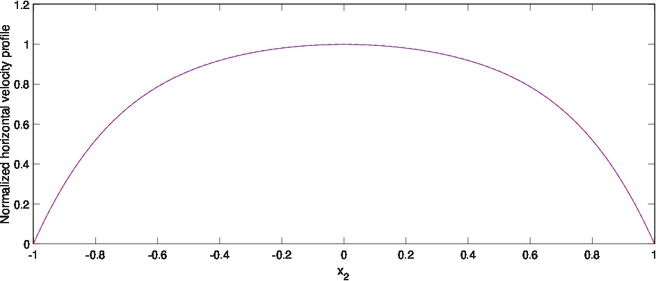
Figure 3: Normalized horizontal velocity profiles obtained for $h=1/96$ (red dashed line) and exact solution (blue solid line) for $n=1/3$.

Figure 4: Normalized horizontal velocity profiles obtained for $h=1/96$ (red dashed line) and exact solution (blue solid line) for $n=1/2$.

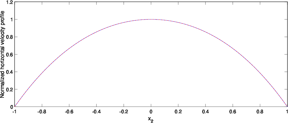
Figure 5: Normalized horizontal velocity profiles obtained for $h=1/96$ (red dashed line) and exact solution (blue solid line) for $n=2/3$.

The numerical results obtained with $h=1/96$ and the actual profiles are shown in Figures 3, 4, and 5 for the steady state horizontal profile of Poiseuille flow. The $L^{2}$-errors of steady numerical solutions in Table 1 show that the expected error order for a $P_{1}$ finite element approximation has been obtained.

(a)

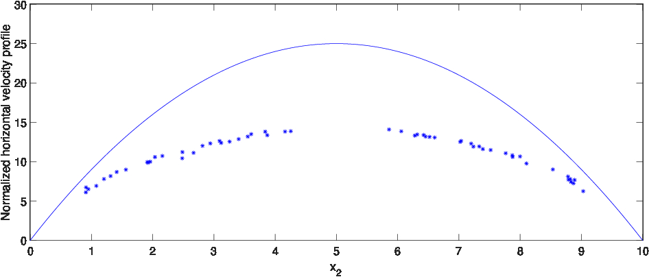
(b) 1

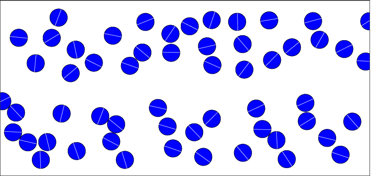
Figure 6: Migration of 56 neutrally buoyant identical particles in the pressure driven flow of a Newtonian fluid without shear thinning ($n=1.0$). (a) Velocity profile of the fluid without particles (top curve) and velocities of particles (bottom curve); (b) particle positions in the channel at time $t=100$.

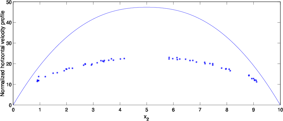
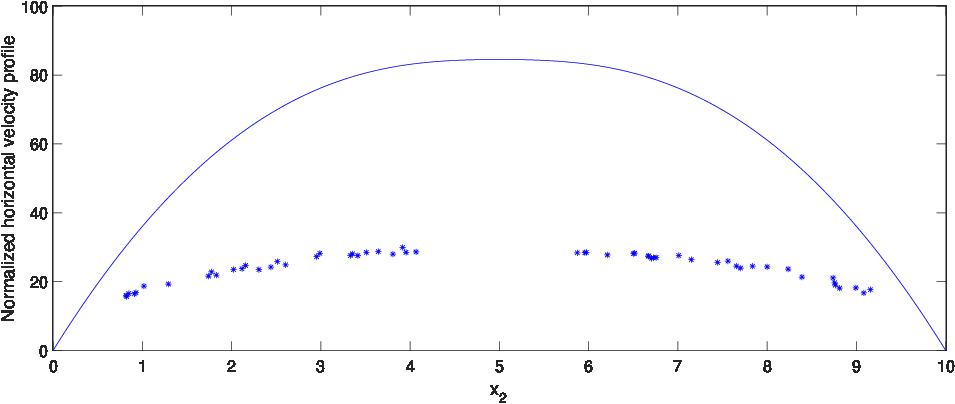
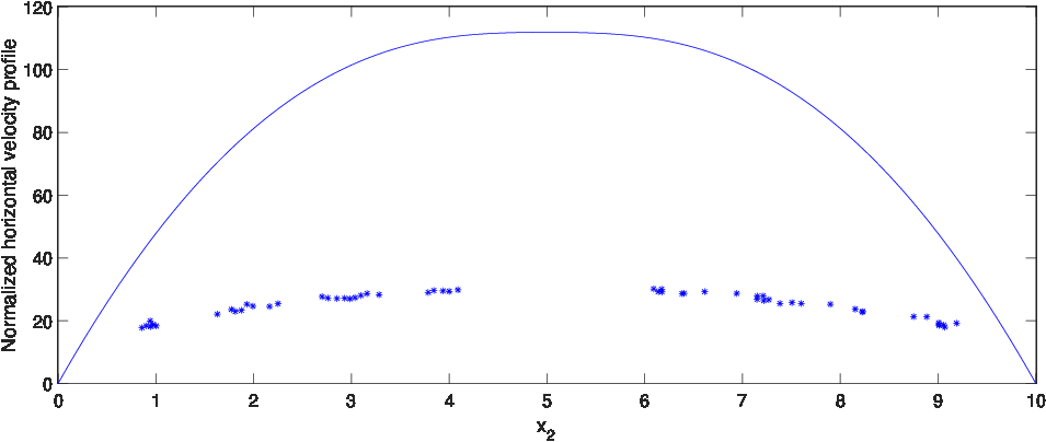
Figure 7: Velocity profile of the fluid without particles and velocities of the 56 particles: $n=0.7$ at $t=42.46$ (top), $n=0.5$ at $t=31.78$ (middle), and $n=0.4$ at $t=27.41$ (bottom).

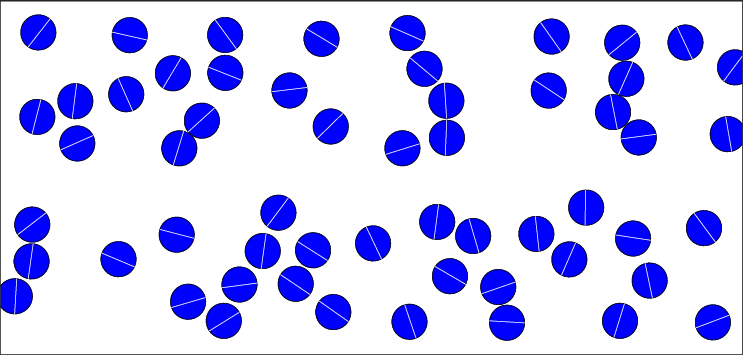
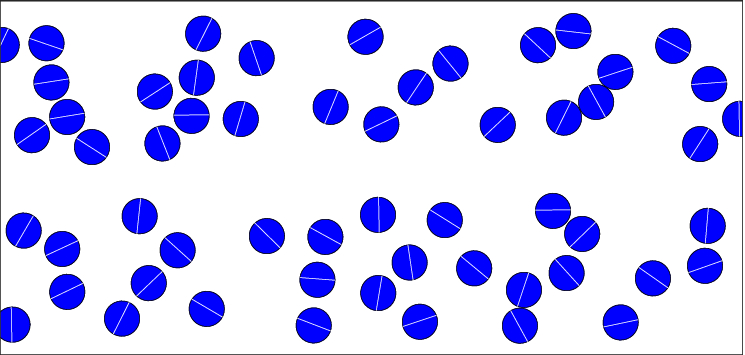
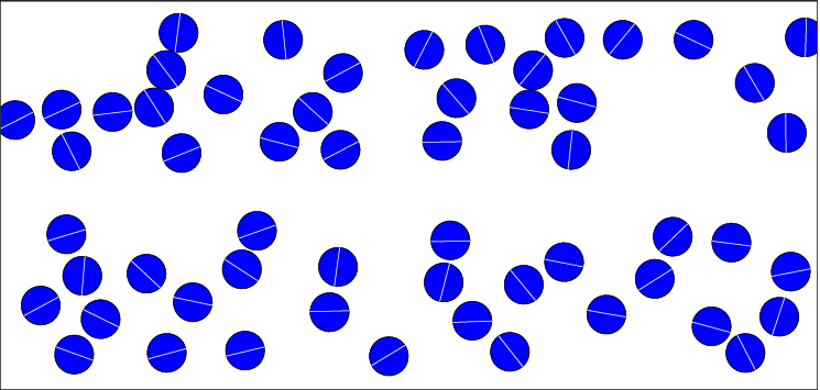
Figure 8: Positions of the 56 neutrally buoyant particles in the pressure driven flow of a shear thinning fluid: $n=0.7$ at $t=42.46$ (top), $n=0.5$ at $t=31.78$ (middle), and $n=0.4$ at $t=27.41$ (bottom).

4.2 On the migration of 56 disks in the Poiseuille flow of a shear thinning fluid

The second validation case we consider concerns the motion and cross stream migration of 56 neutrally buoyant identical circular cylinders in the pressure driven Poiseuille flow of a on-Newtonian shear thinning fluid, which was a test problem studied numerically in [29]. The proposed numerical scheme has been validated by comparing our results with those reported in [29]. The computational domain is $\Omega=(0,21)$ $\times$ $(0,10)$. The initial flow velocity and particle velocities are ${\bf 0}$. The pressure drop is $F_{1}=-2$ so that the maximum horizontal speed is 25 when there is no particle for the Poiseuille flow of a Newtonian fluid with the viscosity $\eta_{0}=1$. For non-Newtonian shear thinning fluids modeled by (7), the viscosity at infinity shear rate is $\eta_{\infty}=0.1\eta_{0}$ and the relaxation time is $\lambda_{3}=1$. The values of the power index $n$ are 0.4, 0.5, and 0.7. The fluid and particle densities are 1. The disk diameter $d$ is 1 and ${\bf u}_{p}(t)$ is ${\bf 0}$ for each disk. The mesh size for the velocity field is $h_{v}=1/16$, while the mesh size for the pressure is $h_{p}=2h_{v}$. The time step is $\triangle t=0.001$.

For the case of a Newtonian fluid without shear thinning ($n=1$), the migration of the disks is shown in Figure 6. There are no disks at the center line and the disks tend to accumulate a distance of 0.6 from the center line of the channel, which is known as the Segre-Silberberg effect (see [30] and [31]). In general, lubrication forces move the particles away from the channel walls while the curvature of the velocity profile moves the particles away from the centerline of the channel. For a small neutrally buoyant ball in a plane Poiseuille flow via the matched asymptotic expansion methods, it was found that the of the fluid without particles and the velocities of the particles at $t=100$ are shown in Figure 6. At $t=100$, the maximum particle velocity is 14.0864, while the maximum fluid velocity without particles is 25 so the slip velocity is 10.9136 near the centerline. In [29] the maximum particle velocity is 15 near the centerline and the maximum slip velocity is 10. Both results are in good agreement.

The velocity profile with shear thinning is quite different from the one at $n=1$ as shown in Figure 7. The effects of shear thinning can be increased by decreasing the power index $n$. The maximum particle velocities are 23.0664, 29.9960, and 30.1694, while the maximum fluid velocities are 47.3956, 84.5356, and 111.9036 for $n=0.7$, 0.5, and 0.4, respectively. Hence we obtain the slip velocities in Table 2 by following the approach given in [29]. Their slip velocities are 23, 54, and 81.4 for $n=0.7$, 0.5, and 0.4, respectively, implying our numerical results are in a good agreement with those in [29]. Due to the Segre-Silberberg effect, the disks separate into two groups (see Figures 7 and 8), the top group and the bottom one according to the particle positions shown in Figure 8. Following these particle separations, there are three particle free zones, the one in the middle (called middle zone), the one next to the top wall (called the top boundary zone), and the one next to the bottom wall (the bottom boundary zone), which can be identified easily from the particle velocity plots in Figure 7. The sizes of these particle free zones are called the gaps and shown in Table 2, in which the average boundary gap is the mean of the two boundary gaps. Due to the shear thinning effect, the disk accumulation is enhanced so that the middle gap of particle free zone increases and the average boundary gap decreases, when decreasing the value of the power index $n$. Our results are consistent with those obtained in [29] qualitatively.

$n$	Slip velocity	Average boundary gap	Middle gap
1	10.9136	0.95167	1.60403
0.7	24.3292	0.85906	1.67752
0.5	54.5396	0.83388	1.80585
0.4	81.7342	0.83313	2.00206

Table 2. The slip velocity, average of gap sizes next to two walls, and gap size in the center of the channel for the power indices $n=1/3$, 1/2, 2/3, and 1.

4.3 On the motion of a self-propelled swimmer

Even Purcell’s scallop theorem [1] rules out reciprocal motion (i.e., strokes with time-reversal symmetry) for effective locomotion in the absence of inertia ($Re=0$) in Newtonian fluids, the motion of a simple reciprocal model swimmer (an asymmetric dumbbell) in a Newtonian fluid at intermediate Reynolds numbers has been studied extensively in [9] and [10]. In this section, we have considered the case of a neutrally buoyant self-propelled swimmer freely moving in a non-Newtonian shear thinning fluid. Such swimmer is formed by two disks of different sizes connecting by a massless spring at their mass centers (see Figure 9). Hence it is an asymmetric long body, but symmetric with respect to the line segment connecting two disk mass centers. The reciprocal motion of two disks with respect to the swimmer mass center is prescribed (see Figure 9 and equation (38)). Due to the asymmetric disk motion with respect to the swimmer mass center, swimmer can move in either directions parallel to the string connecting the two disk mass centers. It is interesting to find out how the shear thinning impacts the swimmer motion. Following the units used in [9], we assume in this section all dimensional quantities are in the physical MKS units.

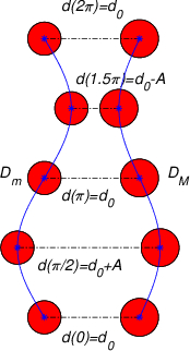
Figure 9: An example of the relative position of the two disks: The reciprocal motion with respect to the swimmer mass center at different time over one period is $d(t)=d_{0}+A\sin(t)$. Disk centers of mass (blue *) are indicated.

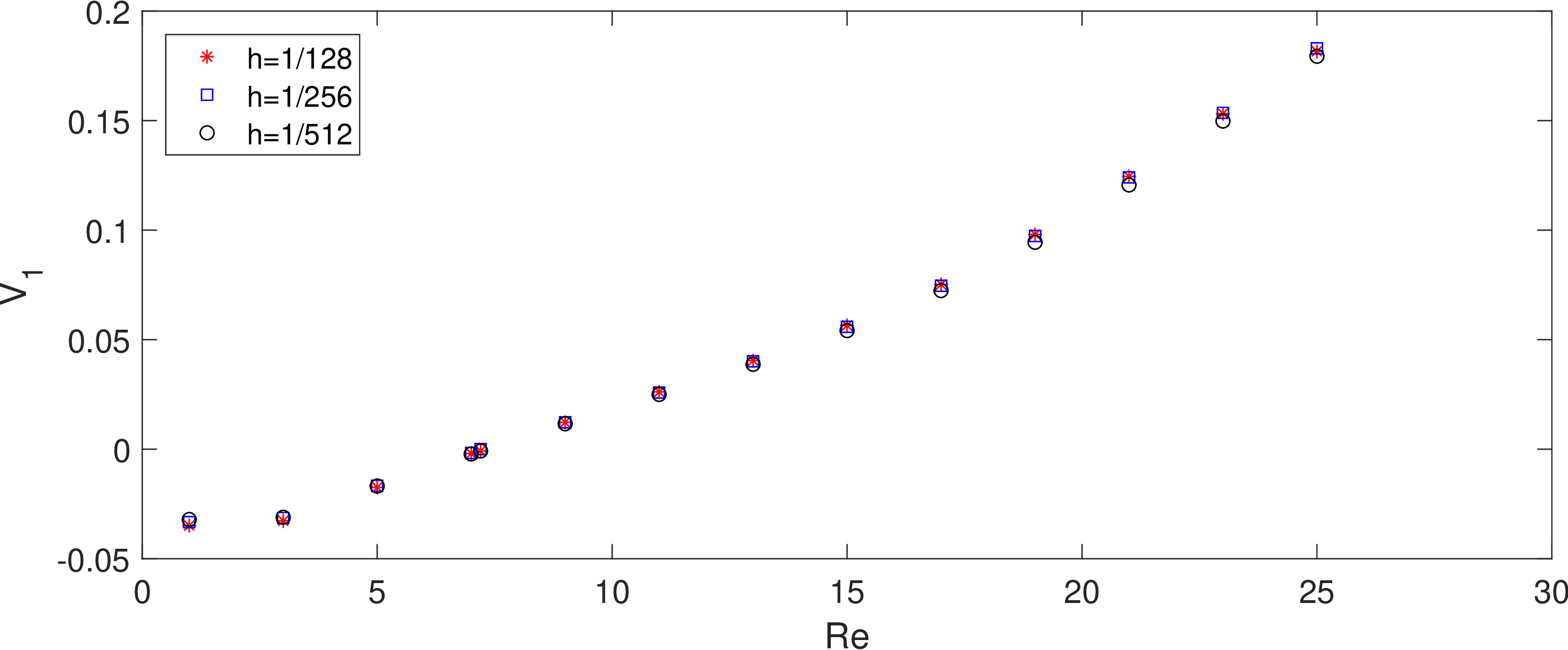
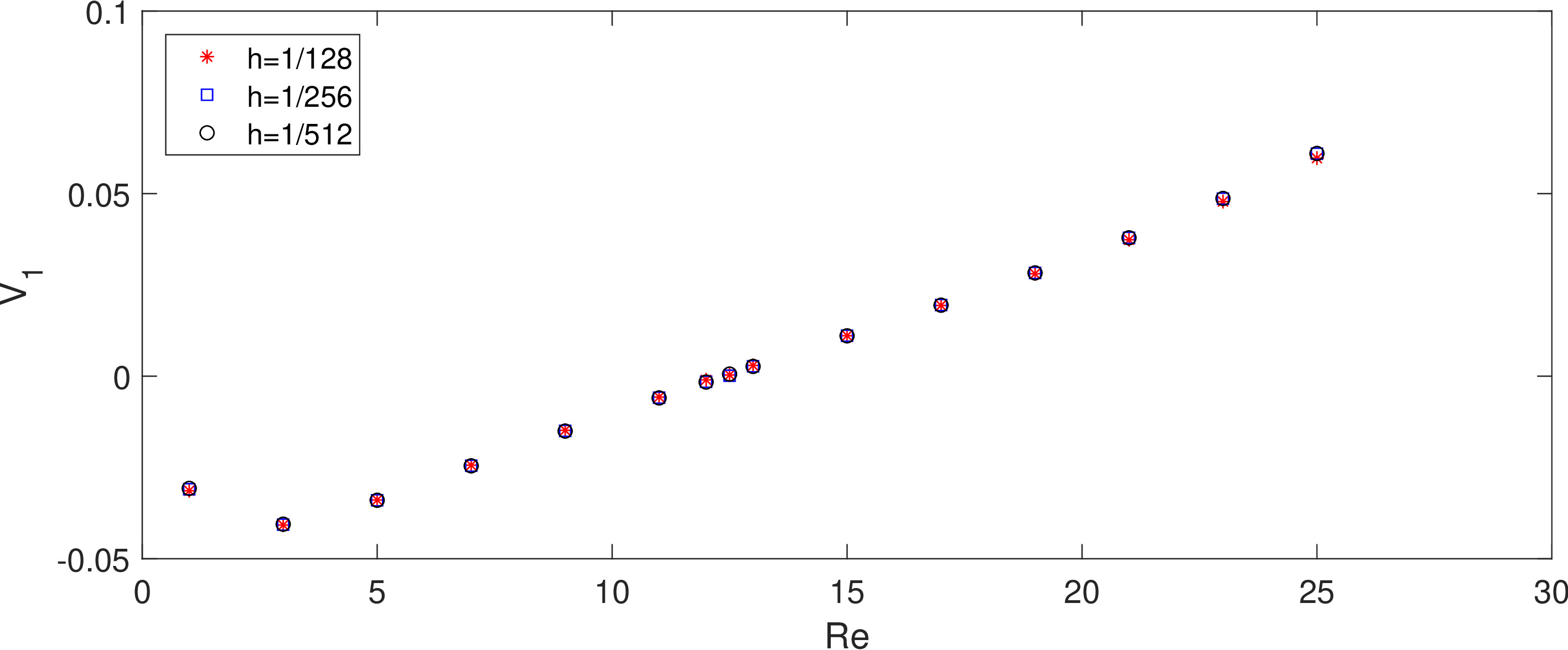
Figure 10: Average horizontal velocity $V_{1}$ of a swimmer versus $Re$ for the power index $n=1$ (top) and 0.8 (bottom).

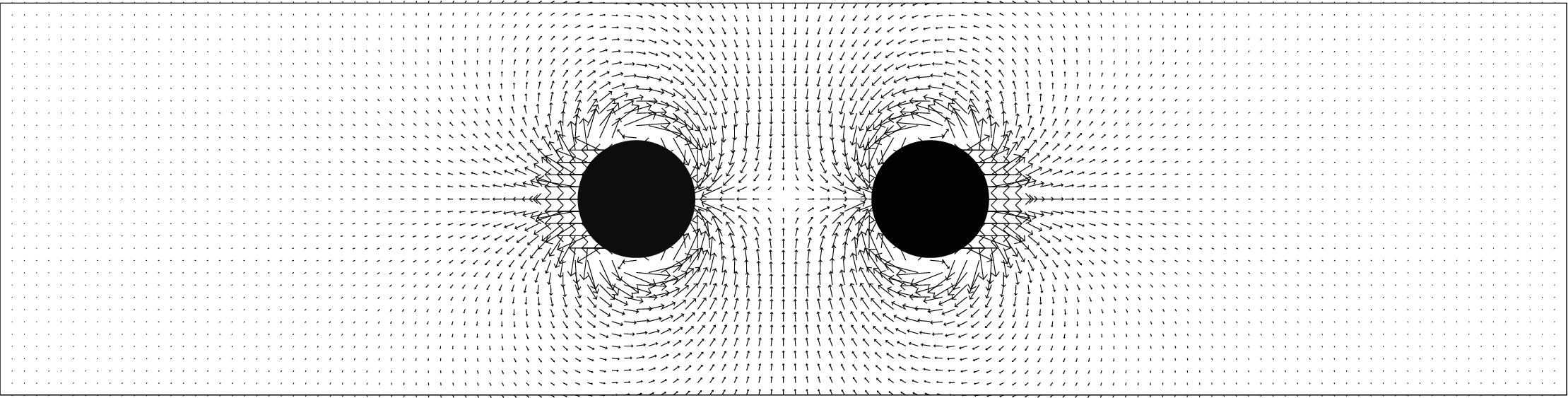
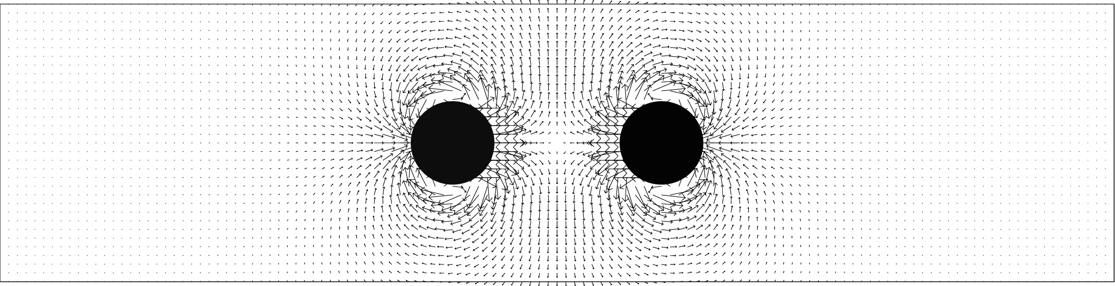
Figure 11: Velocity field next to the swimmer of two same size disks and swimmer position at $t=8$ (top) and 8.05 (bottom) for $Re=15$ and $n=1$.

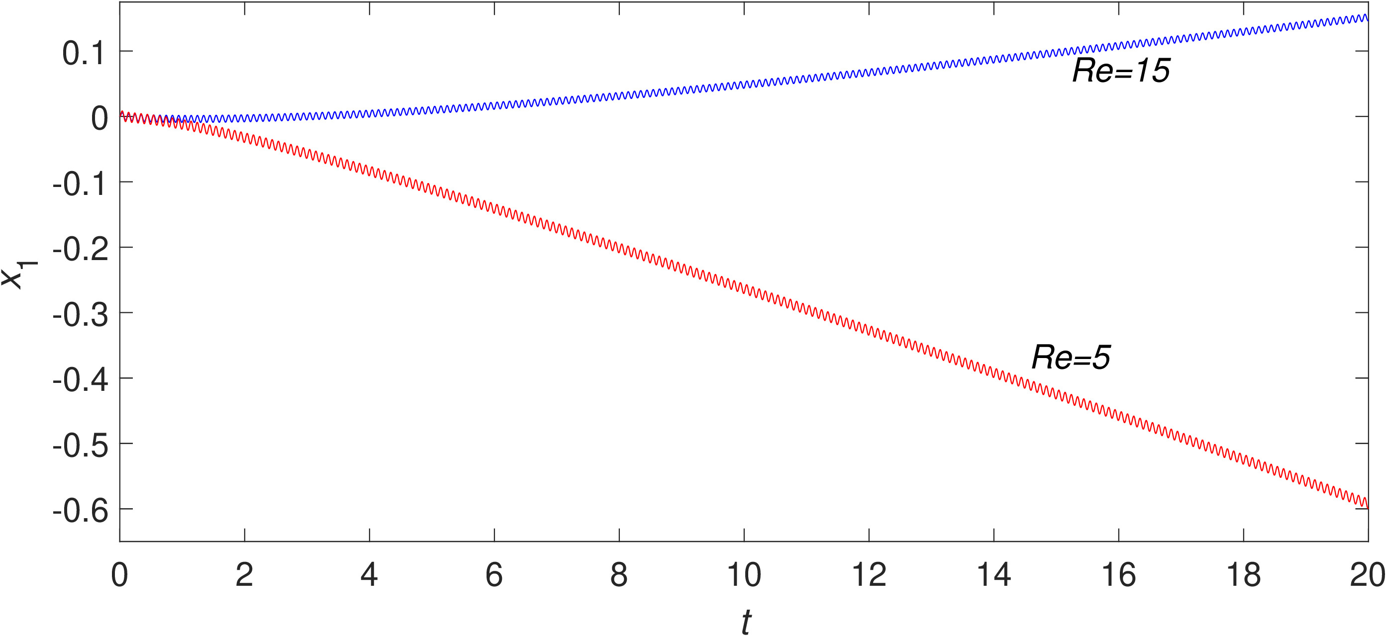
Figure 12: Histories of the horizontal $x_{1}$-position of the swimmer mass center for $Re=5$ and 15 and $n=1$ where the swimmer is formed by two different size disks (see Figure 13).

The computational domain is $\Omega=(-4,4)$ $\times$ $(-4,4)$. The flow velocity is ${\bf 0}$ initially and zero at the boundary of domain $\Omega$. The densities of fluid and swimmer are $10^{3}$, which is the water density. The initial position of the swimmer mass center is at (0,0). The distance between the two disk centers is $d(t)=d_{0}+A\sin(\omega t)$ as in [9] where the equilibrium distance between the two disk centers is $d_{0}=10r_{0}$, the amplitude is $A=r_{0}$, and $r_{0}=0.15$. The angular frequency is $\omega=20\pi$ (so the frequency is 10). The massless spring connecting the two disks is located in the direction parallel to the $x_{1}$ direction. The radius of the larger disk $D_{M}$ is $R_{M}=2r_{0}=0.3$ and that of the smaller disk $D_{m}$ is $R_{m}=r_{0}=0.15$. The amplitude $A$ is $A=A_{M}+A_{m}$ where the component for the larger disk is $A_{M}=\dfrac{AR_{m}^{2}}{R_{M}^{2}+R_{m}^{2}}$ and the one for the smaller disk is $A_{m}=\dfrac{AR_{M}^{2}}{R_{M}^{2}+R_{m}^{2}}$. The Reynolds number is defined by $Re=A_{m}R_{m}\omega/\nu$ (as in [9]) where $\nu$ is the kinetic viscosity of the fluid at zero shear rate. We vary the value of $Re$ to obtain the fluid viscosity at zero shear rate. We have used structured triangular meshes in all simulations. The mesh size for the velocity field is $h_{v}=1/128$, while the mesh size for pressure is $h_{p}=2h_{v}$. The time step is $\triangle t=0.001$. Concerning the shear thinning, the ratio of viscosity at infinity shear rate and the one at zero shear rate is 0.1 and the relaxation time is $\lambda_{3}=1$. The values of the power index $n$ are 0.5, 0.6, 0.7, 0.8, and 0.9.

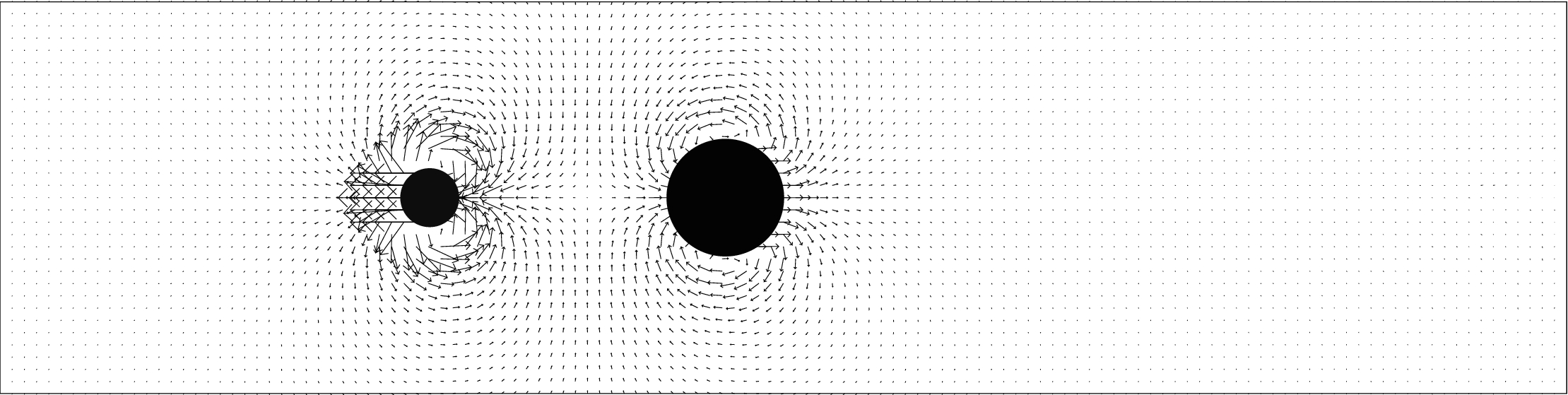
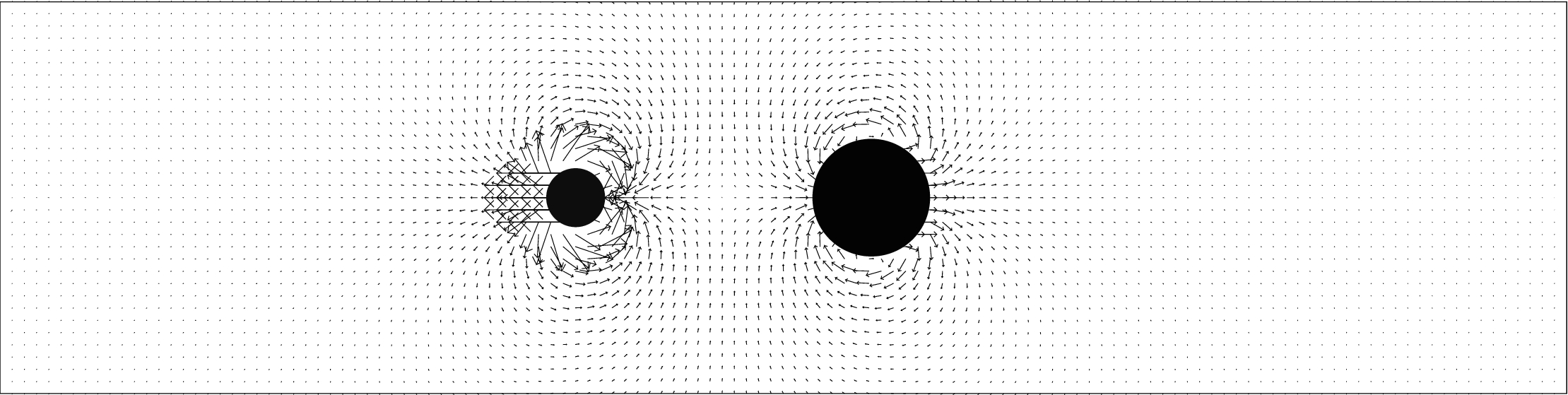
Figure 13: Swimmer position at $t=0$ (top), velocity field next to the swimmer and swimmer position at $t=20$ for $Re=5$ (middle) and 15 (bottom) and $n=1$.

In this section, we have mainly studied the effect of the power index $n$ and of the Reynolds number on the moving direction and speed of the swimmer. In order to focus on the swimmer moving direction, the swimmer is only allowed to freely move in the $x_{1}$-direction. To accommodate this restricted motion and the Dirichlet boundary condition, we have to modify the spaces defined previously as follows

$$W_{0} = \{{\bf v}|{\bf v}\in(H^{1}(\Omega))^{2},\ {\bf v}={\bf 0}\ \text{\it on the boundary of $\Omega$.}\},$$

$$\Lambda_{0}(t) = \{{\boldsymbol{\mu}}|{\boldsymbol{\mu}}\in(H^{1}(B(t)))^{2},<{\boldsymbol{\mu}},{\bf e}_{1}>_{B(t)}=0\},$$

$$W_{0,h} = \{{\bf v}_{h}|{\bf v}_{h}\in(C^{0}(\overline{\Omega}))^{2},\ {\bf v}_{h}|_{T}\in P_{1}\times P_{1},\forall T\in{\mathcal{T}}_{h},$$

$${\bf v}_{h}={\bf 0}\ \text{\it on the boundary}\ \text{\it of $\Omega$}\},$$

$$L^{2}_{0,h} = \{q_{h}|q_{h}\in C^{0}(\overline{\Omega}),\ q_{h}|_{T}\in P_{1},\ \forall T\in{\mathcal{T}}_{2h},\ \int_{\Omega}q_{h}\,d{\bf x}=0\},$$

$$\Lambda_{0,h}(t) = \{\mu_{h}|\mu_{h}\in\Lambda_{h}(t),\ <\mu_{h},{\bf e}_{1}>_{B_{h}(t)}=0\}.$$

Following the above given restricted motion, the reciprocal motion with respect to the swimmer mass center is

(38) $${\bf u}_{p}(t)=\begin{cases}(A_{M}\omega\cos(\omega t),0)^{T},\ \forall{\bf x}\in D_{M},\\ (-A_{m}\omega\cos(\omega t),0)^{T},\ \forall{\bf x}\in D_{m}.\\ \end{cases}$$

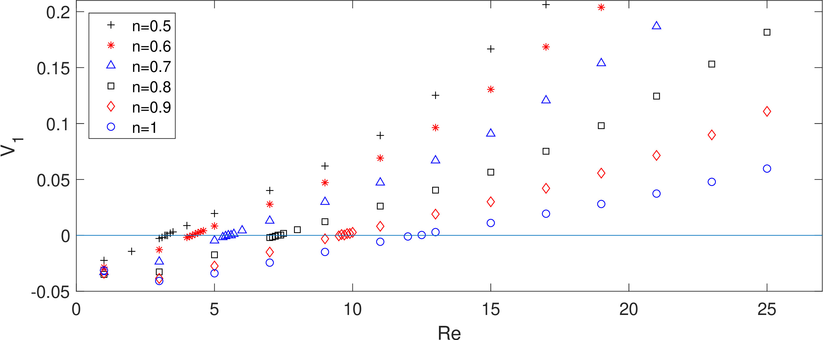
Figure 14: Average horizontal speed $V_{1}$ of a swimmer versus $Re$ for the power index $n=0.5$, 0.6, 0.7, 0.8, 0.9, and 1.

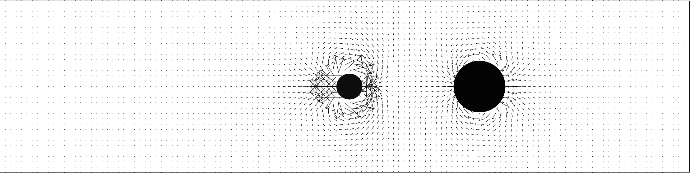
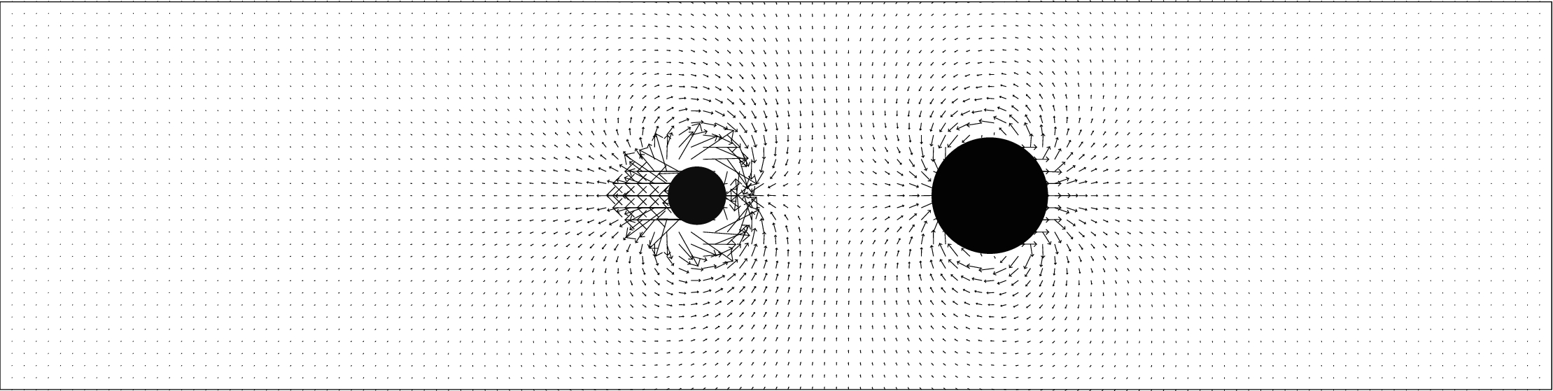
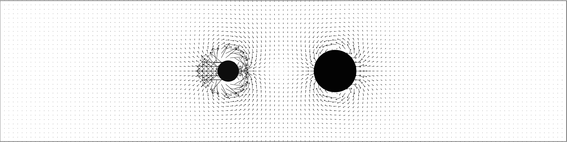
Figure 15: Velocity field next to the swimmer and swimmer position at $t=20$ for $Re=15$ and $n=0.7$ (top), $n=0.8$ (middle), and $n=0.9$ (bottom).

Applying algorithm (21)-(36) (with the subproblem (37) instead of problem (25) for shear thinning fluids) and above discrete spaces, we have studied numerically the motion of two disk swimmer in the $x_{1}$ direction in Newtonian and non-Newtonian fluids. We first show the average velocities of swimmer for different values of $Re$ and two power index values, $n=1$ and 0.8, obtained by the velocity mesh sizes $h=1/128$, 1/256, and 1/512 and time step $\triangle t=0.001$. Each average value was computed from the last twenty periods of horizontal velocity for $0\leq t\leq 20$. All those average velocities for each Reynolds number are in a good agreement as shown in Figure 10.

Let us consider a swimmer of two same size disks, i.e., $R_{m}=R_{M}=2r_{0}=0.3$, suspended in a Newtonian fluid ($n=1$). Due to the symmetry of reciprocal motion of the two same size disks (see Figure 11), the swimmer mass center does not move as expected, at least for $Re=1$, 3, 5, 7, 9, 11, 13, and 15, the cases we have considered. But for the case of two different size disks in a Newtonian fluid with $R_{M}=2r_{0}$ and $R_{m}=r_{0}$ for $r_{0}=0.15$, the swimmer can move in the positive or negative $x_{1}$-direction up to the Reynolds number. As shown in Figure 12, the swimmer mass center oscillates with period 0.1 but moves in the positive (resp., negative) $x_{1}$-direction for $Re=15$ (resp., $Re=5$). There is a critical Reynolds number so that the swimmer moves to the left (resp., right) for $Re<Re_{c}$ (resp., $Re>Re_{c}$) if the larger disk is located on the right side (see the plots in Figures 13 and 14). The critical Reynolds number is about $Re_{c}=12.5$ for the swimmer shown in Figure 13.

But when swimming in a non-Newtonian shear thinning fluid, the average moving speed ($V_{1}$) per period in the positive-$x_{1}$ direction increases when decreasing the value of the power index $n$ as shown in Figures 14 for the power index values, $n=0.5$, 0.6, 0.7, 0.8, 0.9, and 1. Interestingly the average swimming velocity is also slow down when the swimmer moves in the minus-$x_{1}$ direction when decreasing the value of the power index $n$. Thus the swimmer position is further to the right when comparing its position at $t=20$ as in Figure 15. Our computational results show that the shear thinning does have a strong effect on the motion of a swimmer made of two different size disks and the critical Reynolds number decreases for a non-Newtonian shear thinning fluid as the power index value decreases.

5 Conclusions

In this article, a distributed Lagrange multiplier/fictitious domain method has been developed for simulating a non-symmetric (two-disk) particle moving freely in non-Newtonian shear thinning fluids. The Carreau-Bird model is adapted for the fluid shear thinning property. Our numerical methods have been validated by comparing our computed solutions with the recently published exact solutions for Poiseuille flows of non-Newtonian fluids in two dimensions (in ref. [13]). Accurate numerical solutions have been obtained and the $L^{2}$-errors of the velocity field show the expected 2nd order for $P_{1}$ finite elements. For many neutrally buoyant particle cross stream migration in a Poiseuille flow of non-Newtonian shear thinning fluids, the particles migrate away from the wall and center of the channel. The size of the boundary gap decreases and that of the middle gap increases when reducing the power index value. These results are consistent qualitatively with those reported in [29]. Concerning the two-disk swimmer, the effect of shear thinning does let the swimmer move faster when moving in the positive $x_{1}$-direction, i.e., from the smaller to larger disk, and the critical Reynolds number (for changing the moving direction from the left to the right) decreases for smaller value of the power index.

Acknowledgments

We acknowledge the helpful comments and suggestions of Howard H. Hu (University of Pennsylvania).

References

- [1] Purcell EM. Life at low Reynolds number. Am J Phys. 1977;45(1):3-11.
- [2] Lauga E, Powers TR. The hydrodynamics of swimming microorganisms. Rep Prog Phys. 2009;72(9):096601.
- [3] Carreau PJ. Rheological Equations from Molecular Network Theories. Transactions of the Society of Rheology. 1972;16(1):99-127.
- [4] Bird RB, Armstrong RC, Hassager O. Dynamics of polymeric liquids, Volume 1 Fluid Mechanics. 2 ed. New York, NY:John Wiley and Sons; 1987.
- [5] Lauga E. Life at high Deborah number. Europhysics Letters. 2009;86(6):64001.
- [6] Normand T, Lauga E. Flapping motion and force generation in a viscoelastic fluid. Phys Rev E. 78 (2008) 061907.
- [7] Montenegro-Johnson TD, Smith DJ, Loghin D. Physics of rheologically enhanced propulsion: different strokes in generalized Stokes. Phys Fluids. 2013;25(8):081903.
- [8] Qiu T, Lee TC, Mark AG, Morozov KI, Münster R, Mierka O,et al. Swimming by reciprocal motion at low Reynolds number. Nature communications. 2014;5(1):1-8.
- [9] Dombrowski T, Jones SK, Katsikis G, Bhalla APS, Griffith BE, Klotsa D. Kinematics of a simple reciprocal model swimmer at intermediate Reynolds numbers. Phys Rev Fluids. 2020;5(6):063103.
- [10] Dombrowski T, Klotsa D. Transition in swimming direction in a model self-propelled inertial swimmer. Phys Rev Fluids. 2019;4(2):021101.
- [11] Huang PY, Feng J, Hu HH, Joseph DD. Direct simulation of the motion of solid particles in Couette and Poiseuille flows of viscoelastic fluids. J Fluid Mech. 1997;343:73-94.
- [12] Huang PY, Hu HH, Joseph DD. Direct simulation of the motion of elliptic particles in Oldroyd-B fluids. J Fluid Mech. 1998;362:297-325.
- [13] Griffiths PT. Non-Newtonian channel flow—exact solutions. IMA J Appl Math. 2020;85(2):263-279.
- [14] Pan T-W, Glowinski R. Direct simulation of the motion of neutrally buoyant circular cylinders in plane Poiseuille flow. J Comp Phys. 2002;181(1):260-279.
- [15] Pan T-W, Glowinski R. Direct simulation of the motion of neutrally buoyant balls in a three-dimensional Poiseuille flow. C R Mecanique, Acad Sci Paris. 2005;333(12):884-895.
- [16] Yang BH, Wang J, Joseph JJ, Hu HH, Pan T-W, Glowinski R. Migration of a sphere in tube flow. J Fluid Mech. 2005;540:109-131.
- [17] Pan T-W, Li A, Glowinski R. Numerical study of equilibrium radial positions of neutrally buoyant balls in circular Poiseuille flows. Phys Fluids. 2021;33(3):033301.
- [18] Bristeau MO, Glowinski R, Periaux J. Numerical methods for the Navier-Stokes equations. Applications to the simulation of compressible and incompressible viscous flow. Computer Physics Reports. 1987;6(1-6):73-187.
- [19] Glowinski R. Finite element methods for incompressible viscous flow. In: Ciarlet PG, Lions JL eds. Handbook of Numerical Analysis, vol. IX. Amsterdam: North-Holland; 2003:3-1176.
- [20] Chorin AJ, Hughes TJR, McCracken MF, Marsden JE. Product formulas and numerical algorithms. Comm Pure Appl Math. 1978;31(2):205-256.
- [21] Glowinski R, Osher SJ, Yin W eds. Operator-Splitting in Communications and Imaging, Sciences, and Engineering. Gewerbestrasse, Switzerland:Springer;2016.
- [22] Glowinski R, Pan T-W, Hesla T, Joseph DD. A distributed Lagrange multiplier/fictitious domain method for particulate flows. Int J Multiphase Flow. 1999;25(5):755-794.
- [23] Glowinski R, Pan T-W, Hesla T, Joseph DD, Periaux J. A fictitious domain approach to the direct numerical simulation of incompressible viscous flow past moving rigid bodies: Application to particulate flow. J Comput Phys. 2001;169(2):363-426.
- [24] Glowinski R, Pan T-W, Periaux J. Distributed Lagrange multiplier methods for incompressible flow around moving rigid bodies. Comput Methods Appl Mech Engrg. 1998;151(1-2):181-194.
- [25] J. Adams, P. Swarztrauber, and R. Sweet, FISHPAK: A package of FORTRAN subprograms for the solution of separable elliptic partial differential equations (The National Center for Atmospheric Research, Boulder, CO, 1980).
- [26] Dean EJ, Glowinski R. A wave equation approach to the numerical solution of the Navier-Stokes equations for incompressible viscous flow. C R Acad Sci Paris, Série 1-Mathematics. 1997;325(7):783-791.
- [27] Pan T-W, Glowinski R. A projection/wave-like equation method for the numerical simulation of incompressible viscous fluid flow modeled by the Navier-Stokes equations. Computational Fluid Dynamics Journal. 2000;9:28-42.
- [28] Whiteman JR, Goodsell G. A survey of gradient superconvergence for finite element approximation to second order elliptic problems on triangular tetrahedral meshes. In: Whiteman JR, ed. The Mathematics of Finite Elements and Applications VII. London:Academic Press; 1991:55-74.
- [29] Huang PY, Joseph DD. Effects of shear thinning on migration of neutrally buoyant particles in pressure driven flow of Newtonian and viscoelastic fluids. J. Non-Newtonian Fluid Mech. 2000;90(2-3):159-185.
- [30] Segré G., Silberberg A. Radial particle displacements in Poiseuille flow of suspensions. Nature. 1961;189(4760):209-210.
- [31] Segré G, Silberberg A. Behavior of macroscopic rigid spheres in Poiseuille flow. Part I, Determination of local concentration by statistical analysis of particle passages through crossed light beams. J Fluid Mech. 1962;14(1):115-157.