Generalizing Graph Neural Networks on Out-Of-Distribution Graphs

Abstract

Graph Neural Networks (GNNs) are proposed without considering the agnostic distribution shifts between training graphs and testing graphs, inducing the degeneration of the generalization ability of GNNs on Out-Of-Distribution (OOD) settings. The fundamental reason for such degeneration is that most GNNs are developed based on the I.I.D hypothesis. In such a setting, GNNs tend to exploit subtle statistical correlations existing in the training set for predictions, even though it is a spurious correlation. This learning mechanism inherits from the common characteristics of machine learning approaches. However, such spurious correlations may change in the wild testing environments, leading to the failure of GNNs. Therefore, eliminating the impact of spurious correlations is crucial for stable GNN models. To this end, in this paper, we argue that the spurious correlation exists among subgraph-level units and analyze the degeneration of GNN in causal view. Based on the causal view analysis, we propose a general causal representation framework for stable GNN, called StableGNN. The main idea of this framework is to extract high-level representations from raw graph data first and resort to the distinguishing ability of causal inference to help the model get rid of spurious correlations. Particularly, to extract meaningful high-level representations, we exploit a differentiable graph pooling layer to extract subgraph-based representations by an end-to-end manner. Furthermore, inspired by the confounder balancing techniques from causal inference, based on the learned high-level representations, we propose a causal variable distinguishing regularizer to correct the biased training distribution by learning a set of sample weights. Hence, GNNs would concentrate more on the true connection between discriminative substructures and labels. Extensive experiments are conducted on both synthetic datasets with various distribution shift degrees and eight real-world OOD graph datasets. The results well verify that the proposed model StableGNN not only outperforms the state-of-the-arts but also provides a flexible framework to enhance existing GNNs. In addition, the interpretability experiments validate that StableGNN could leverage causal structures for predictions.

1 Introduction

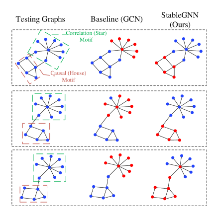
Figure 1: Visualization of subgraph importance for “house” motif classification task, produced by the vanilla GCN model and StableGNN when most of training graphs containing “house” motifs with “star” motifs. The red subgraph indicates the most important subgraph used by the model for prediction (generated by GNNExplainer (Ying et al., 2019)). Due to the spurious correlation, the GCN model tends to focus more on “star” motifs while our model focuses mostly on “house” motifs. For more cases of testing graph, please refer to Figure 5.

Graph Neural Networks (GNNs) are powerful deep learning algorithms on graphs with various applications (Scarselli et al., 2008; Kipf & Welling, 2016; Veličković et al., 2017; Hamilton et al., 2017). One major category of applications is the predictive task over entire graphs, i.e., graph-level task, such as molecular graph property prediction (Hu et al., 2020; Lee et al., 2018; Ying et al., 2018), scene graph classification (Pope et al., 2019), and social network category classification (Zhang et al., 2018; Ying et al., 2018), etc. The success could be attributed to the non-linear modeling capability of GNNs, which extracts the useful information from raw graph data and encodes them into the graph representation in a data-driven fashion.

The basic learning diagram of existing GNNs is to learn the parameters of GNNs from the training graphs, and then make predictions on unseen testing graphs. The most fundamental assumption to guarantee the success of such learning diagram is the I.I.D. hypothesis, i.e., training and testing graphs are independently sampled from the identical distribution (Liao et al., 2020). However, in reality, such a hypothesis is hardly satisfied due to the uncontrollable generation mechanism of real data, such as data selection biases, confounder factors or other peculiarities (Bengio et al., 2019; Engstrom et al., 2019; Su et al., 2019; Hendrycks & Dietterich, 2019). The testing distribution may incur uncontrolled and unknown shifts from the training distribution, called Out-Of-Distribution (OOD) shifts (Sun et al., 2019; Krueger et al., 2021), which makes most GNN models fail to make stable predictions. As reported by OGB benchmark (Hu et al., 2020), GNN methods will occur a degeneration of 5.66% to 20% points when splitting the datasets according to the OOD settings, i.e., splitting structurally different graphs into training and testing sets.

Essentially, for general machine learning models, when there incurs a distribution shift, the main reason for the degeneration of accuracy is the spurious correlation between the irrelevant features and the category labels. This kind of spurious correlations is intrinsically caused by the unexpected correlations between irrelevant features and relevant features for a given category (Zhang et al., 2021; Lake et al., 2017; Lopez-Paz et al., 2017). For graph-level tasks that we focus on in this paper, as the predicted properties of graphs are usually determined by the subgraph units (e.g., groups of atoms and chemical bonds representing functional units in a molecule) (Ying et al., 2018; 2019; Jin et al., 2020), we define one subgraph unit could be one relevant feature or irrelevent feature with graph label. Taking the classification task of “house” motif as an example, as depicted in Figure 1, where the label of graph is labeled by whether the graph has a "house" motif and the first column represents the testing graphs. The GCN model is trained on the dataset where “house” motifs coexist with “star” motifs in most training graphs. With this dataset, the structural features of “house” motifs and “star” motifs would be strongly correlated. This unexpected correlation leads to spurious correlation between structural features of “star” motifs with the label “house”. And the second column of Figure 1 shows the visualization of the most importance subgraph used by the GCN for prediction (shown with red color and generated by GNNExplainer (Ying et al., 2019)). As a result, the GCN model tends to use such spurious correlation, i.e., "star" motif, for prediction. When encountering graphs without “star” motif, or other motifs (e.g., “diamond” motifs) with “star” motifs, the model is prone to make false predictions (See Section 5.1).

To improve the OOD generalization ability of GNNs, one important way is to make GNNs get rid of such subgraph-level spurious correlation. However, it is not a trivial task, which will face the two following challenges: (1) How to explicitly encode the subgraph-level information into graph representation? As the spurious correlation usually exists between subgraphs, it is necessary to encode such subgraph information into the graph representation, so that we could develop decorrelation method based on the subgraph-level representation. (2) How to remove the spurious correlation among the subgraph-level representations? The nodes in same type of subgraph units may exist correlation, for example, the information of ‘N’ atom and ‘O’ atom in ‘NO2’ groups of molecular graphs may be encoded into different dimensions of learned embedding, but they act as an integrated whole and such correlations are stable across unseen testing distributions. Hence, we should not remove the correlation between the interior variables of one kind of subgraphs and only need to remove the spurious correlation between subgraph-level variables.

To address these two challenges, we propose a novel causal representation framework for graph, called StableGNN, which takes the advantages of both the flexible representation ability of GNNs and the distinguishing ability for spurious correlations of causal inference methods. In terms of the first challenge, we propose a graph high-level variable learning module that employs a graph pooling layer to map nearby nodes to a set of clusters, where each cluster will be one densely-connected subgraph unit of original graph. Moreover, we theoretically prove that the semantic meanings of clusters would be aligned across graphs by a ordered concatenation operation. Given the aligned high-level variables, to overcome the second challenge, we analyze the degeneration of GNNs in causal view and propose a novel causal variable distinguishing regularizer to decorrelate each high-level variable pair by learning a set of sample weights. These two modules are jointly optimized in our framework. Furthermore, as shown in Figure 1, StableGNN can effectively partial out the irrelevant subgraphs (i.e., “star” motif) and leverage truly relevant subgraphs (i.e., “house” motif) for predictions.

In summary, the major contributions of the paper are as follows:

• To our best knowledge, we firstly study the OOD generalization problem on GNNs for graph-level task, which is a key direction to apply GNNs to wild non-stationary environments.

• We propose a general causal representation learning framework for GNNs, jointly learning the high-level representation with the causal variable distinguisher, which could learn an invariant relationship between the graph causal variables with the labels. And our framework is general to be adopted to various base GNN models to help them get rid of spurious correlations.

• Comprehensive experiments are conducted on both synthetic datasets and real-world OOD graph datasets. The effectiveness, flexibility and interpretability of the proposed framework have been well validated with the convincing results.

2 Related Work

In this section, we discuss three main categories closely related with our work: graph neural networks, causal representation learning and stable learning.

2.1 Graph Neural Networks

Graph neural networks are powerful deep neural networks that could perform on graph data directly (Scarselli et al., 2008; Kipf & Welling, 2016; Veličković et al., 2017; Hamilton et al., 2017; Zhang et al., 2018; Lee et al., 2018). Most of these approaches fit within the framework of “neural message passing” (Gilmer et al., 2017). In the message passing framework, a GNN is regarded as a message passing algorithm where node representations are iteratively calculated from the features of their neighborhood nodes using a differentiable aggregation function. GNNs have been applied to a wide variety of tasks, including node classification (Kipf & Welling, 2016; Veličković et al., 2017; Hamilton et al., 2017; Bo et al., 2021), link prediction (Schlichtkrull et al., 2018; Zhang & Chen, 2018), and graph classification (Zhang et al., 2018; Lee et al., 2018). For graph classification, the task we majorly focus on here, the major challenge in applying GNNs is how to generate the representation of the entire graph. Common approaches to this problem is simply summing up or averaging all the node embedding in final layer. Several literatures argue that such simply operation will greatly ignore high-level structure that might be presented in the graph, and then propose to learn the hierarchical structure of graph in an end-to-end manner (Zhang et al., 2018; Ying et al., 2018; Lee et al., 2019; Gao & Ji, 2019). Although these methods have achieved remarkable results in I.I.D setting, they largely ignore the generalization ability in OOD setting, which is crucial for real applications.

2.2 Causal Representation Learning

Recently, Schölkopf et al. (Schölkopf et al., 2021) publish a survey paper, towards causal representation learning, and point out that causality, with its focus on representing structural knowledge about the data generating process that allows interventions and changes, can contribute towards understanding and resolving some limitations of current machine learning methods. Traditional causal discovery and reasoning assume that the units are random variables connected by a causal graph. However, real-world observations are not structured into these units, for example, graph data we focus on is a kind of unstructured data. Thus for this kind of data, causal representation learning generally consists of two steps: (1) inferring the abstract/high-level causal variables from available low-level input features, and (2) leveraging the causal knowledge as inductive bias to learn the causal structure of high-level variables. After learning the causal system, the causal relationship is robust to irrelevant interventions and changes on data distributions. Based on this idea, Invariant Risk Minimization (IRM) framework (Arjovsky et al., 2019; Rosenfeld et al., 2020; Kamath et al., 2021) proposes a regularization that enforce model learn an invariant representation across environments. The representation learning part plays the role of extracting high-level representation from low-level raw features, and the regularization encodes the causal knowledge that causal representation should be invariant across environments into the representation learning. Despite the IRM framework could learn the representations that have better OOD generalization ability, the requirement that domains should be labeled hinders the IRM methods from real applications. To overcome such dilemma, some methods are proposed to implicitly learn domains from data (Qiao et al., 2020; Matsuura & Harada, 2020; Wang et al., 2019), but they implicitly assume the training data is formed by balanced sampling from latent domains. However, in reality, due to the uncontrollable data generation process, the assumption could be easily violated, leading to the degeneration of these methods. More importantly, all these methods are mainly designed for tabular or image data, thus they cannot capture the intrinsic properties of graphs.

2.3 Stable Learning

To improve the feasibility of IRM based methods, a series of researches on stable learning are proposed (Kuang et al., 2018; 2020). These methods mainly bring the ideas from the causal effect estimation (Angrist & Imbens, 1995) into machine learning models. Particularly, Shen et al. (Shen et al., 2018) propose a global confounding balancing regularizer that helps the logistic regression model to identify causal features, whose causal effect on outcome are stable across domains. To make the confounder balancing much easier in high-dimensional scenario, Kuang et al. (Kuang et al., 2018) utilize the autoencoder to encode the high-dimensional features into low-dimensional representation. Furthermore, (Kuang et al., 2020) and (Shen et al., 2020) demonstrate that decorrelating relevant and irrelevant features can make a linear model produce stable prediction under distribution shifts. The decorrelation operation actually has the same effect with confounder balancing, as the global confounder balancing regularizer tends to make every pair of treatment and confounder independent. But they are all developed based on the linear framework. Recently, Zhang et al. (Zhang et al., 2021) extend decorrelation into deep CNN model to tackle more complicated data types like images. This method pays much attention to eliminating the non-linear dependence among features, but the feature learning part is largely ignored. We argue that it is important to develop an effective high-level representation learning method to extract variables with appropriate granularity for the targeted task, so that the causal variable distinguishing part could develop on meaningful causal variables.

Figure 2: Causal graph for data generation process. Gray nodes and white nodes mean the unobserved latent variables and the observed variables, respectively.

3 Problem Formulation

Notations. In our paper, for a vector $\mathbf{v}$, $\mathbf{v}_{i}$ represents the $i$-th element of $\mathbf{v}$. For any matrix $\mathbf{X}$, let $\mathbf{X}_{i,}$ and $\mathbf{X}_{,j}$ represent the $i$-th row and the $j$-th column in $\mathbf{X}$, respectively. $\mathbf{X}_{i,j}$ represents the $j$-th element of $i$-th row vector of $\mathbf{X}$. $\mathbf{X}_{,j:k}$ means the submatrix of $\mathbf{X}$ from $j$-th column to $(k-1)$-th column. And for any italic uppercase letter, such as $X$, it will represent a random variable.

Problem 1.

OOD Generalization Problem on Graphs. Given the training graphs $\mathcal{G}_{train}=\{(G_{1},Y_{1}),\cdots,(G_{n},Y_{n})\}$, where $G_{i}$ means the $i$-th graph data in training set and $Y_{i}$ is the corresponding label, the task is to learn a GNN model $h_{\theta}(\cdot)$ with parameter $\theta$ to precisely predict the label of testing graphs $\mathcal{G}_{test}$, where the distribution $\Psi(\mathcal{G}_{train})\neq\Psi(\mathcal{G}_{test})$. And in the OOD setting, we do not know the distribution shifts from training graphs to unseen testing graphs.

We utilize a causal graph of the data generation process, as shown in Figure 2, to illustrate the fundamental reason to cause the distribution shifts on graphs. As illustrated in the figure, the observed graph data $G$ is generated by the unobserved latent cause $Z$ and $M$. $Z$ is a set of relevant variables and the label $Y$ is mainly determined by $Z$. $M$ is a set of irrelevant variables which does not decisive for label $Y$. During the unseen testing process in the real world, the variable $M$ could change, but the causal relationship P($Y$|$Z$) is invariant across environments. Taking the classifying mutagenic property of a molecular graph (Luo et al., 2020) as an example, $G$ is a molecular graph where the nodes are atoms and the edges are the chemical bonds between atoms, and $Y$ is the class label, e.g., whether the molecule is mutagenic or not. The whole molecular graph $G$ is an effect of relevant latent causes $Z$ such as the factors to generate nitrogen dioxide (NO2) group, which has an determinative effect on the mutagenicity of molecule, and the effect of irrelevant variable $M$, such as the carbon ring which exist more frequently in mutagenic molecule but not determinative (Luo et al., 2020). If we aim to learn a GNN model that is robust to unseen change on $M$, such as carbon exists in the non-mutagenic molecule, one possible way is to develop a representation function $f(\cdot)$ to recover $Z$ and $M$ from $G$, and learn a classifier $g(\cdot)$ based on $Z$, so that the invariant causal relationship $P(Y|Z)$ could be learned.

4 The Proposed Method

4.1 Overview

The basic idea of our framework is to design a causal representation learning method that could extract meaningful graph high-level variables and estimate their true causal effects for graph-level tasks. As depicted in Figure 3, the proposed framework mainly consists of two components: the graph high-level variable learning component and causal variable distinguishing component. The graph high-level variable learning component first employs a graph pooling layer that learns the node embedding and maps nearby nodes into a set of clusters. Then we get the cluster-level embeddings through aggregating the node embeddings in the same cluster, and align the cluster semantic space across graphs through an ordered concatenation operation. The cluster-level embeddings act as the high-level variables for graphs. After obtaining the high-level variables, we develop a sample reweighting component based on Hilbert-Schmidt Independence Criterion (HSIC) measure to learn a set of sample weights that could remove the non-linear dependences among multiple multi-dimensional embeddings. As the learned sample weights could generate a pseudo-distribution with less spurious correlation among cluster-level variables, we utilize the weights to reweight the GNN loss. Thus the GNN model trained on this less biased pseudo-data could estimate causal effect of each high-level variable with the label more precisely, resulting in better generalization ability in wild environments.

Figure 3: The overall architecture of the proposed StableGNN.

4.2 Graph High-level Variable Learning

As the goal of this component is to learn a representation that could represent original subgraph unit explicitly, we adopt a differentiable graph pooling layer that could map densely-connected subgraphs into clusters by an end-to-end manner. And then we theoretically prove that the semantic meaning of the learned high-level representations could be aligned by a simple ordered concatenation operation.

High-level Variable Pooling. To learn node embedding as well as map densely connected subgraphs into clusters, we exploit the DiffPool layer (Ying et al., 2018) to achieve this goal by learning a cluster assignment matrix based on the learned embedding in each pooling layer. Particularly, as GNNs could smooth the node representations and make the representation more discriminative, given the input adjacency matrix $\mathbf{A}$, also denoted as $\mathbf{A}^{(0)}$ in this context, and the node features $\mathbf{F}$ of a graph, we first use an embedding GNN module to get the smoothed embeddings $\mathbf{F}^{(0)}$:

$$\mathbf{F}^{(0)}=\text{GNN}^{(0)}_{\text{embed}}(\mathbf{A}^{(0)},\mathbf{F}),$$ (1)

where $\text{GNN}^{(0)}_{\text{embed}}(\cdot,\cdot)$ is a three-layer GNN module, and the GNN layer could be GCN (Kipf & Welling, 2016), GraphSAGE (Hamilton et al., 2017), or others. Then we develop a pooling layer based on the smoothed representation $\mathbf{F}^{(0)}$. In particular, we first generate node representation at layer 1 as follows:

$$\mathbf{Z}^{(1)}=\text{GNN}^{(1)}_{\text{embed}}(\mathbf{A}^{(0)},\mathbf{F}^{(0)}).$$ (2)

As nodes in the same subgraph would have similar node features and neighbor structure and GNN could map the nodes with similar features and structural information into similar representation, we also take the node embeddings $\mathbf{F}^{(0)}$ and adjacency matrix $\mathbf{A}^{(0)}$ into a pooling GNN to generate a cluster assignment matrix at layer $1$, i.e., the clusters of original graph:

$$\mathbf{S}^{(1)}=\text{softmax}(\text{GNN}^{(1)}_{\text{pool}}(\mathbf{A}^{(0)},\mathbf{F}^{(0)})),$$ (3)

where $\mathbf{S}^{(1)}\in\mathbb{R}^{n_{0}\times n_{1}}$, and $\mathbf{S}^{(1)}_{i,}$ represents the cluster assignment vector of $i$-th node, and $\mathbf{S}^{(1)}_{,j}$ corresponds to the all nodes’ assignment probabilities on $j$-th cluster at the layer $1$. $\text{GNN}_{\text{pool}}^{(1)}(\cdot,\cdot)$ is also a three-layer GNN module, and the output dimension of $\text{GNN}_{\text{pool}}^{(1)}(\cdot,\cdot)$ is a pre-defined maximum number of clusters at layer $1$ and is a hyperparameter. And the appropriate number of clusters could be learned in an end-to-end manner. The maximum number of clusters in the last pooling layer should be the number of high-level variables we aim to extract. The softmax function is applied in a row-wise fashion to generate the cluster assignment probabilities for each node at layer $1$.

After obtaining the assignment matrix $\mathbf{S}^{(1)}$, we could know the assignment probability of each node on the predefined clusters. Hence, based on the assignment matrix $\mathbf{S}^{(1)}$ and learned the node embedding matrix $\mathbf{Z}^{(1)}$, we could the a new coarsened graph, where the nodes are the clusters learned by this layer and edges are the connectivity strength between each pair of clusters. Particularly, the new matrix of embeddings is calculated by the following equation:

$$\mathbf{F}^{(1)}={\mathbf{S}^{(1)}}^{\mathrm{T}}\mathbf{Z}^{(1)}\in\mathbb{R}^{n_{1}\times d}.$$ (4)

This equation aggregates the node embedding $\mathbf{Z}^{(1)}$ according to the cluster assignment $\mathbf{S}^{(1)}$, generating embeddings for each of the $n_{1}$ clusters. Similarly, we generate a coarsened adjacency matrix as follows.

$$\mathbf{A}^{(1)}={\mathbf{S}^{(1)}}^{\mathrm{T}}\mathbf{A}^{(1)}\mathbf{S}^{(1)}\in\mathbb{R}^{n_{1}\times n_{1}}.$$ (5)

For all the operations with superscript (1), it is one DiffPool unit and it is denoted as $(\mathbf{A}^{(1)},\mathbf{F}^{(1})=\text{DiffPool}(\mathbf{A}^{(0)},\mathbf{F}^{(0)})$. For any DiffPool layer $l$, it could be denoted as $(\mathbf{A}^{(l)},\mathbf{F}^{(l)})=\text{DiffPool}(\mathbf{A}^{(l-1)},\mathbf{F}^{(l-1)})$. In particular, we could stack multiple DiffPool layers to extract the deep hierarchical structure of the graph.

High-level Representation Alignment. After stacking $L$ graph pooling layers, we could get the most high-level cluster embedding $\mathbf{F}^{(L)}\in\mathbb{R}^{{n_{L}}\times d}$, where $\mathbf{F}^{(L)}_{i,}$ represents the $i$-th high-level representation of the corresponding subgraph in the original graph. As our target is to encode subgraph information into graph representation and $\mathbf{F}^{(L)}$ has explicitly encoded each densely-conntected subgraph information into each row of $\mathbf{F}^{(L)}$, we propose to utilize the embedding matrix $\mathbf{F}^{(L)}$ to represent the high-level variables. However, due to the Non-Euclidean property of graph data, for the $i$-th learned high-level representations $\widehat{\mathbf{F}}^{(L)}_{i,}$ and $\widetilde{\mathbf{F}}^{(L)}_{i,}$ from two graphs $\widehat{G}$ and $\widetilde{G}$, respectively, their semantic meaning may not matched, e.g., $\widehat{\mathbf{F}}^{(L)}_{i,}$ and $\widetilde{\mathbf{F}}^{(L)}_{i,}$ may represent ring carbon and NO2 group in two molecular graphs, respectively. To match the semantic meaning of learned high-level representation across graphs, we propose to concatenate the high-level variables by the order of row index of high-level embedding matrix for each graph:

$$\mathbf{h}=\text{concat}(\mathbf{F}^{(L)}_{1,},\mathbf{F}^{(L)}_{2,},\cdots,\mathbf{F}^{(L)}_{n_{L},}),$$ (6)

where $\mathbf{h}\in\mathbb{R}^{n_{L}d}$ and $\text{concat}(\cdot)$ means concatenation operation by the row axis. Moreover, we stack $m$ high-level representations for a mini-batch with $m$ graphs to obtain the embedding matrix $\mathbf{H}\in\mathbb{R}^{m\times n_{L}d}$:

$$\mathbf{H}=\text{stack}(\mathbf{h}_{1},\mathbf{h}_{2},\cdots,\mathbf{h}_{m}),$$ (7)

where $\text{stack}(\cdot)$ means the stacking operation by the row axis, and $\mathbf{H}_{i,}$ means the high-level representation for the $i$-th graph in the mini-batch. $\mathbf{H}_{i,(k-1)d:kd}$ means $k$-th high-level representation of $i$-th graph. Hence, to prove the semantic alignment of any two high-level representations $\mathbf{H}_{i,}$ and $\mathbf{H}_{j,}$, we need to demonstrate that the semantic meanings of $\mathbf{H}_{i,(k-1)d:kd}$ and $\mathbf{H}_{j,(k-1)d:kd}$ are aligned for all $k\in[1,n_{L}]$. To this end, we first prove the permutation invariant property of DiffPool layer.

Lemma 1.

Permutation Invariance (Ying et al., 2018). Given any permutation matrix $\mathbf{P}\in\{0,1\}^{n\times n}$, if $\mathbf{P}\cdot\text{GNN}(\mathbf{A},\mathbf{F})=\text{GNN}(\mathbf{P}\mathbf{A}\mathbf{P}^{\mathrm{T}},\mathbf{P}\mathbf{F})$ (i.e., the GNN method used is permutation equivariant), then $\text{DiffPool}(\mathbf{A},\mathbf{F})=\text{DiffPool}(\mathbf{P}\mathbf{A}\mathbf{P}^{\mathrm{T}},\mathbf{P}\mathbf{F})$.

Proof.

Following (Keriven & Peyré, 2019), a function $f:\mathbb{R}^{n\times d}\rightarrow\mathbb{R}^{n\times l}$: is invariant if $f(\textbf{F},\textbf{X})=f(\textbf{PFP}^{\mathrm{T}},\textbf{PF})$, i.e, the permutation will not change node representation and the node order in the learned matrix. A function $f:\mathbb{R}^{n\times d}\rightarrow\mathbb{R}^{n\times l}$: is equivariant if $f(\textbf{A},\textbf{F})=\textbf{P}\cdot f(\textbf{PAP}^{\mathrm{T}},\textbf{PF})$, i.e, the permutation will not change the node representation but the order of nodes in matrix will be permuted. The permutation invariant aggregator functions such as mean pooling and max pooling ensures that the basic model can be trained and applied to arbitrarily ordered node neighborhood feature sets, i.e, permutation equivariant. Therefore, the Eq. (2) and  (3) are the permutation equivariant by the assumption that the GNN module is permutation equivariant. And since any permutation matrix is orthogonal, i.e., $\mathbf{P}^{\mathrm{T}}\mathbf{P}=\mathbf{I}$, applying this into Eq. (4) and (5), we have:

$$\mathbf{F}^{(1)}={\mathbf{S}^{(1)}}^{\mathrm{T}}\mathbf{P}^{\mathrm{T}}\mathbf{P}\mathbf{Z}^{(1)},$$ (8)

$$\mathbf{A}^{(1)}={\mathbf{S}^{(1)}}^{\mathrm{T}}\mathbf{P}^{\mathrm{T}}\mathbf{P}\mathbf{A}^{(1)}\mathbf{P}\mathbf{P}^{\mathrm{T}}\mathbf{S}^{(1)}.$$ (9)

Hence, DiffPool layer is permutation invariant. ∎

After proving the permutation invariant property of single graph, we then illustrate the theoretical results for the semantic alignment of learned high-level representation across graphs.

Theorem 1.

Semantic Alignment of High-level Variables. Given any two graphs $G_{i}=(\mathbf{A}_{i},\mathbf{F}_{i})$ and $G_{j}=(\mathbf{A}_{j},\mathbf{F}_{j})$, the semantic space of high-level representations $\mathbf{H}_{i,}$ and $\mathbf{H}_{j,}$ learned by a series of shared DiffPool layers is aligned.

Proof.

WL-test (Leman & Weisfeiler, 1968) is widely used in graph isomorphism checking: if two graphs are isomorphic, they will have the same multiset of WL colors at any iteration. GNNs could be viewed a continuous approximation to the WL test, where they both aggregate signal from neighbors and the trainable neural network aggregators is analogy to hash function in WL-test (Zhang et al., 2018). Therefore, the outputs of GNN module are exactly the continuous WL colors. Then the embeddings value between any two graphs in the same layer will be in the same WL color space. The color space would represent a semantic space. Hence, the semantic meaning of each column of the learned assignment matrices $\mathbf{S}_{i}^{(l)}$ and $\mathbf{S}_{j}^{(l)}$ of graphs $G_{i}$ and $G_{i}$ would be aligned, e.g., the $k$-th column would represent carbon ring structure in all molecule graphs. Due to the permutation invariant property of DiffPool layer, according to Eq. (8), the input graph with any node order will map its carbon ring structure signal into the $k$-th high-level representation, i.e., the $k$-th high-level representation of $\mathbf{H}_{i,(k-1)d:kd}$ and $\mathbf{H}_{j,(k-1)d:kd}$. Hence, the semantic meaning of $\mathbf{H}_{i,.}$ and $\mathbf{H}_{j,.}$ is aligned. ∎

4.3 Causal Variable Distinguishing Regularizer

So far the variable learning part extracts all the high-level representations for all the densely-connected subgraphs regardless of whether it is relevant with the graph label due to causal relation or spurious correlation. In this section, we first analyze the reason leading to the degeneration of GNNs on OOD scenarios in causal view and then propose the Causal Variable Distinguishing (CVD) regularizer with sample reweighting technique.

(a) Confounder balancing framework.

(b) Multiple multi-dimensional confounder balancing framework.

Figure 4: Causal view on GNNs.

Revisiting on GNNs in Causal View. As described in Section 3, our target is to learn a classifier $g(\cdot)$ based on the relevant variable $Z$. To this end, we need to distinguish which variable of learned high-level representation $\mathbf{H}$ belongs to $Z$ or $M$. The major difference of $Z$ and $M$ is whether they have casual effect on $Y$. For a graph-level classification task, after learning the graph representation, it will be fed into a classifier to predict its label. The prediction process could be represented by the causal graph with three variables and their relationships, as shown in Figure 4(a), where $T$ is a treatment variable, $Y$ is label/outcome variable, and $X$ is the confounder variable, which has effect both on treatment variable and outcome variable. The path $T\rightarrow Y$ represents the target of GNNs that aims to estimate the causal effect of the one learned variable $T$ (e.g., $i$-th high-level representation $\mathbf{H}_{,(i-1)d:id}$ ) on $Y$. Meanwhile, other learned variables (e.g., $j$-th high-level representation $\mathbf{H}_{,(j-1)d:jd}$) will act as counfounder $X$. Due to the existence of spurious correlation of subgraphs, there has spurious correlation between their learned embeddings. Hence, there incurs a path between $X$ and $T$. And because GNNs also employ the confounder (e.g., the representation of carbon ring) for prediction, there exists a path $X\rightarrow Y$. Hence, these two paths form a backdoor path between $X$ and $Y$ (i.e., $T\leftarrow X\rightarrow Y$) and induce the spurious correlation between $T$ and $Y$. And the spurious correlation will amplify the true correlation between treatment variable and label, and may change in testing environments. Under this scenario, existing GNNs cannot estimate the causal effect of subgraphs accurately, so the performance of GNNs will be degenerate when the spurious correlation change in the testing phase. Confounding balancing techniques (Hainmueller, 2012; Zubizarreta, 2015) correct the non-random assignment of treatment variable by balancing the distributions of confounder across different treatment levels. Because moments can uniquely determine a distribution, confounder balancing methods directly balance the confounder moments by adjusting weights of samples (Athey et al., 2016; Hainmueller, 2012). The sample weights $\mathbf{w}$ for binary treatment scenario are learnt by:

$$\mathbf{w}=\mathop{\arg\min}_{\mathbf{w}}||\sum_{i:T_{i}=1}\mathbf{w}_{i}\cdot\mathbf{X}_{i,}-\sum_{j:T_{j}=0}\mathbf{w}_{j}\cdot\mathbf{X}_{j,}||_{2}^{2},$$ (10)

where $\mathbf{X}$ is the confounder matrix and $\mathbf{X}_{i,}$ is the confounder vector for $i$-th graph. Given a binary treatment feature $T$, $\sum_{i:T_{i}=1}\mathbf{w}_{i}\cdot\mathbf{X}_{i,}$ and $\sum_{j:T_{j}=0}\mathbf{w}_{j}\cdot\mathbf{X}_{j,}$ refer to the mean value of confounders on samples with and without treatment, respectively. After confounder balancing, the dependence between $X$ and $T$ (i.e., $T\leftarrow X$) would be eliminated, thus the correlation between the treatment variable and the output variable will represent the causal effect (i.e., $X\rightarrow Y$).

Moreover, for a GNN model, we have little prior knowledge on causal relationships between the learned high-level variables $\{\mathbf{H}_{,0:d},\cdots,\mathbf{H}_{,(n_{L}-1)d:n_{L}d}\}$, thus have to set each learned high-level variable as treatment variable one by one, and the remaining high-level variables are viewed as confounding variables, e.g, $\mathbf{H}_{,0:d}$ is set as treatment variable and $\{\mathbf{H}_{,d:2d},\cdots,\mathbf{H}_{,(n_{L}-1)d:n_{L}d}\}$ are set as confounders. Note that for a particular treatment variable, previous confounder balancing techniques are mainly designed for a single-dimensional treatment feature as well as the confounder usually consists of multiple variables where each variable is a single-dimensional feature. In our scenario, however, as depicted in Figure 4(b), we should deal with the confounders which are composed of multiple multi-dimensional confounder variables $\{X^{(1)},\cdots,X^{(p)}\}$, where each multi-dimensional confounder variable corresponds to one of learned high-level representations $\{\mathbf{H}_{,0:d},\cdots,\mathbf{H}_{,(n_{L}-1)d:n_{L}d}\}$. The multi-dimensional variable unit usually has integrated meaning such as representing one subgraph, so it is unnecessary to remove the correlation between the treatment variable with each of feature $\mathbf{H}_{,i}$ in one multi-dimensional feature unit, e.g., $\mathbf{H}_{,0:d}$. And we should only remove the subgraph-level correlation between treatment variable $T$ with multiple multi-dimensional variable units $\{X^{(1)},\cdots,X^{(p)}\}$. One possible way to achieve this goal is to learn a set of sample weights that balance the distributions of all confounding variables for the targeted treatment variable, as illustrated in Figure 4(b), i.e., randomizing the assignment of treatment $T$ with confounders $\{X^{(1)},\cdots,X^{(p)}\}$. The sample weights $\mathbf{w}$ could be learnt by the following multiple multi-dimensional confounder balancing objective:

$$\mathbf{w}=\mathop{\arg\min}_{\mathbf{w}}\sum_{k=1}^{p}||\sum_{i:T_{i}=1}\mathbf{w}_{i}\cdot\mathbf{X}_{i,}^{(k)}-\sum_{j:T_{j}=0}\mathbf{w}_{j}\cdot\mathbf{X}_{j,}^{(k)}||_{2}^{2},$$ (11)

where $\mathbf{X}^{(k)}$ is the embedding matrix for $k$-th confounding variable $X^{(k)}$.

Weighted Hilbert-Schmidt Independence Criterion. Since above confounder balancing method is mainly designed for binary treatment variable, which needs the treatment value to divide the samples into treated or control group, it is hard to apply to the continuous multi-dimensional variables learned by GNNs. Inspired by the intuition of confounder balancing is to remove the dependence between the treatment with the corresponding confounding variables, thus we propose to remove dependence between continuous multi-dimensional random variable $T$ with each of confounder in $\{X^{(1)},\cdots,X^{(p)}\}$. Thus we first need to measure the degree of dependence between them. And it is feasible to resort to HSIC measure (Song et al., 2007). For two random variables $U$ and $V$ and kernel $k$ and $l$, HSIC is defined as $\text{HSIC}^{k,l}(U,V):=||C^{k,l}_{UV}||^{2}_{\text{HS}}$, where $C^{k,l}$ is cross-covariance operator in the Reproducing Kernel Hilbert Spaces (RKHS) of $k$ and $l$ (Gretton et al., 2005), an RKHS analogue of covariance matrices. $||\cdot||_{\text{HS}}$ is the Hilbert-Schmidt norm, a Hilbert-space analogue of the Frobenius norm. For two random variables $U$ and $V$ and radial basis function (RBF) kernels $k$ and $l$, $\text{HSIC}^{k,l}(U,V)=0$ if and only if $U\perp V$. To estimate $\text{HSIC}^{k,l}(U,V)$ with finite sample, we employ a widely used estimator $\text{HSIC}^{k,l}_{0}(U,V)$ (Gretton et al., 2005) with $m$ samples, defined as:

$$\text{HSIC}^{k,l}_{0}(U,V)=(m-1)^{-2}tr(\mathbf{KPLP}),$$ (12)

where $\mathbf{K},\mathbf{L}\in\mathbb{R}^{m\times m}$ are RBF kernel matrices containing entries $\mathbf{K}_{ij}=k(U_{i},U_{j})$ and $\mathbf{L}_{ij}=l(V_{i},V_{j})$, and $\mathbf{P}=\mathbf{I}-m^{-1}\mathbf{1}\mathbf{1}\in\mathbb{R}^{m\times m}$ is a centering matrix which projects onto the space orthogonal to the vector $\mathbf{1}$.

To eliminate the dependence between the high-level treatment representation with the corresponding confounders, sample reweighting techniques could generate a pseudo-distribution which has less dependence between variables (Zhang et al., 2021; Zou et al., 2020). We propose a sample reweighting method to eliminate the dependence between high-level variables, where the non-linear dependence is measured by HSIC.

We use $\mathbf{w}\in\mathbb{R}^{m}_{+}$ to denote a set of sample weights and $\sum^{m}_{i=1}\mathbf{w}_{i}=m$. For any two random variables $U$ and $V$, we first utilize the random initialized weights to reweight these two variables:

$$\hat{U}=(\mathbf{w}\cdot\mathbf{1}^{\mathrm{T}})\odot U,$$ (13)

$$\hat{V}=(\mathbf{w}\cdot\mathbf{1}^{\mathrm{T}})\odot V.$$ (14)

Substituting $\hat{U}$ and $\hat{V}$ into Eq. (12), we obtain the weighted HSIC value:

$$\hat{\text{HSIC}}^{k,l}_{0}(U,V,\mathbf{w})=(m-1)^{-2}tr(\mathbf{\hat{K}P\hat{L}P}),$$ (15)

where $\hat{\mathbf{K}},\hat{\mathbf{L}}\in\mathbb{R}^{m\times m}$ are weighted RBF kernel matrices containing entries $\hat{\mathbf{K}}_{ij}=k(\hat{U}_{i},\hat{U}_{j})$ and $\hat{\mathbf{L}}_{ij}=l(\hat{V}_{i},\hat{V}_{j})$. Specially, for treatment variable $\mathbf{H}_{,0:d}$ and its corresponding multiple confounder variables $\{\mathbf{H}_{,d:2d},\cdots,\mathbf{H}_{,(n_{L}-1)d:n_{L}d}\}$, we share the sample weights $\mathbf{w}$ across multiple confounders and propose to optimize $\mathbf{w}$ by:

$$\mathbf{w}^{*}=\mathop{\arg\min}_{\mathbf{w}\in\Delta_{m}}\sum_{1<p<n_{L}}\hat{\text{HSIC}}^{k,l}_{0}(\mathbf{H}_{,0:d},\mathbf{H}_{,(p-1)d:pd},\mathbf{w}),$$ (16)

where $\Delta_{m}=\{\mathbf{w}\in\mathbb{R}^{n}_{+}|\sum_{i=1}^{m}\mathbf{w}_{i}=m\}$ and we utilize $\mathbf{w}=\text{softmax}(\mathbf{w})$ to satisfy this constraint. Hence, reweighting training samples with the optimal $\mathbf{w}^{*}$ can mitigate the dependence between high-level treatment variable with confounders to the greatest extent.

Global Multi-dimensional Variable Decorrelation. Note that the above method is to remove the correlation between a single treatment variable $\mathbf{H}_{,0:d}$ with the confounders $\{\mathbf{H}_{,d:2d},\cdots,\mathbf{H}_{,(n_{L}-1)d:n_{L}d}\}$. However, we need to estimate the casual effect of all the learned high-level representations $\{\mathbf{H}_{,0:d},\mathbf{H}_{,d:2d},\cdots,\mathbf{H}_{,(n_{L}-1)d:n_{L}d}\}$. As mentioned above, we need to set each high-level representation as treatment variable and the remaining high-level representations as confounders, and remove the dependence between each treatment variable with the corresponding confounders. One effective way to achieve this goal is to remove the all the dependence between variables. Particularly, we learn a set of sample weights that globally remove the dependence between each pair of high-level representations, defined as follows

$$\mathbf{w}^{*}=\mathop{\arg\min}_{\mathbf{w}\in\Delta_{m}}\sum_{1\leq i<j\leq n_{L}}\hat{\text{HSIC}}^{k,l}_{0}(\mathbf{H}_{,(i-1)d:id},\mathbf{H}_{,(j-1)d:jd},\mathbf{w}).$$ (17)

As we can see from Eq. (17), the global sample weights $\mathbf{w}$ simultaneously reduce the dependence among all high-level representations.

4.4 Weighted Graph Neural Networks

In the traditional GNN model, the parameters of the model are learned on the original graph dataset $\mathcal{G}=\{G_{1},\cdots,G_{m}\}$. Because the sample weights $\mathbf{w}$ learned by the causal variable distinguishing regularizer are capable of globally decorrelating the high-level variables, we propose to use the sample weights to reweight the GNN loss, and iteratively optimize sample weights $\mathbf{w}$ and the parameters of weighted GNN model as follows:

$$f^{(t+1)},g^{(t+1)}=\mathop{\arg\min}_{f,g}\sum_{i=1}^{m}\mathbf{w}^{(t)}_{i}L(g(f(\mathbf{A}_{i},\mathbf{F}_{i})),y_{i}),$$ (18)

$$\mathbf{w}^{(t+1)}=\mathop{\arg\min}_{\mathbf{w}^{(t+1)}\in\Delta_{m}}\sum_{1\leq i<j\leq n_{L}}\hat{\text{HSIC}}^{k,l}_{0}(\mathbf{H}_{,(i-1)d:id}^{(t+1)},\mathbf{H}^{(t+1)}_{,(j-1)d:jd},\mathbf{w}^{(t)}),$$ (19)

where $f(\cdot)$ is representation part of our model and its output is the high-level representation $\mathbf{H}$, $\mathbf{H}^{(t+1)}=f^{(t+1)}(\mathbf{A},\mathbf{F})$, $t$ represents the iteration number, $g(\cdot)$ is a linear prediction layer, and $L(\cdot,\cdot)$ represents the loss function depends on which task we target. For classification task, cross entropy loss is used, and for regression task, least squared loss is used. Initially, $\mathbf{w}^{(0)}=(1,1,\cdots,1)^{\mathrm{T}}$ in each mini-batch. In the training phase, we iteratively optimize sample weights and model parameters with Eq. (18) and (19). During the inference phase, the predictive model directly conducts prediction based on GNN model without any calculation of sample weights. The detailed procedure of our model is shown in Algorithm 1.

Although StableGNN still performs on dataset $\mathcal{G}$, the weight $\mathbf{w}_{i}$ of each graph is no longer same. This weight adjusts the contribution of each graph in the mini-batch loss, so that the GNN parameters are learned on the dataset that each high-level features are decorrelated which can better learn the true correlation between relevant features and labels.

Input: Training graphs $\mathcal{G}_{train}=\{(G_{1},y_{1}),\cdots,(G_{N},y_{N})\}$;

Training Epoch:$Epoch$;

Decorrelation Epoch: $DecorEpoch$;

Output: Learned GNN model;

1 while $t<Epoch$ do

2       for 1 to BatchNumber do

3             Forward propagation to generate $\mathbf{H}$;

4             for 1 to $DecorEpoch$ do

5                   Optimize sample weights $\mathbf{w}$ via Eq. (19);

6                  

7             end for

8            Back propagate with weighted GNN loss to update $f$ and $g$ via Eq. (18);

9            

10       end for

11      

12 end while

Algorithm 1 Training process of StableGNN

Discussion. Our proposed framework, StableGNN, aims to relive the distribution shifts problem by causal representation learning diagram in a general way. Specially, a new causal representation learning for graph that seamless integrates the power of representation learning and causal inference is proposed. For the representation learning part, we could utilize various state-of-the-art graph pooling layer (Zhang et al., 2018; Ying et al., 2018; Lee et al., 2019; Gao & Ji, 2019) to extract high-level representations, nevertheless the main intuition of our work is that we should learn high-level meaningful representation rather than meaningless mixed representation in our proposed learning diagram. This point is key for meaningful and effective causal learning, which is validated in Section 5.2. Moreover, we believe that this general framework has the potential to spur the causal representation in other areas, such as for images, we could extract high-level object representation first and utilize causal inference techniques to incorporate knowledge into the learning framework.

Time Complexity Analysis. As the proposed framework consists of two parts, we analyze them separately. For graph high-level part, to cluster nodes, although it requires additional computation of an assignment matrix, we observed that the Diffpool layer did not incur substantial additional running time in practice. The reason is that each DiffPool layer reduces the size of graphs by extracting a coarser high-level representation of the graph, which speeds up the graph convolution operation in the next layer. For CVD regularizer, given $n_{L}$ learned high-level representation, the complexity of compute HSIC value of each pair of high-level variable is $\mathcal{O}(m^{2})$ (Song et al., 2012), where $m$ is the batch size. Hence, for each batch, the computation complexity of CVD regularizer is $\mathcal{O}(tn_{L}(n_{L}-1)m^{2})$, where $t$ is the number of epochs to optimize $\mathbf{w}$ and $n_{L}$ is a very small number.

5 Experiments

In this section, we evaluate our algorithm on both synthetic and real-world datasets, comparing with state-of-the-arts.

Model Configurations. In our experiments, the GNN layer used for DiffPool layer is built on top of the GraphSAGE (Hamilton et al., 2017) or GCN (Kipf & Welling, 2016) layer, to demonstrate that our framework can be applied on top of different GNN models. We use the “max pooling” variant of GraphSAGE. One DiffPool layer is used for all the datasets and more sophisticated hierarchical layers could be learned by stacking multiple DiffPool layers. For our model, StableGNN-SAGE/GCN refers to using GraphSAGE/GCN as base model, respectively. All the models are trained with same learning rate mode and the model for prediction is selected based on the epoch with best validation performance.

5.1 Experiments on Synthetic Data

To better verify the advantages of StableGNN on datasets with different degree of distribution shifts between training set and testing set, we generate the synthetic datasets with clear generation process so that the biased degree of dataset is controllable.

Dataset. We aim to generate a graph classification dataset that has a variety of distribution shifts from training dataset to testing dataset. Inspired by recently studies on GNN explanation (Ying et al., 2019; Lin et al., 2021), we utilize motif as subgraph of graphs. We first generate a base subgraph for each graph, that is, each positive graph has a “house”-structured network motif and each negative graph has a motif that is randomly drawn from 4 candidate motifs (i.e., star, clique, diamond and grid motifs). Hence, the “house” motif is the causal structure that causally determine the label. To inject spurious correlation, $\mu*100\%$ of positive graphs will be added “star” motif and remaining positive and negative graph will randomly add a non-causal motif from 4 candidate motifs. The node features are drawn from same uniform distribution for all nodes. We set $\mu$ as {0.6, 0.7, 0.8, 0.9} to get four spurious correlation degrees for training set. And we set $\mu=0.5$ to generate OOD validation set and $\mu=0.25$ to generate unbiased testing dataset. The larger $\mu$ for training set means there incurs a larger distribution shift between training and testing set. The resulting graphs are further perturbed by adding edges from the vertices of the first motif to one of the vertices of the second motif in each graph with probability 0.25. The number of training samples is 2000, and for validation and testing set is 1000.

Experimental Settings and Metrics. As the synthetic data has known generating mechanism and our model is based on the GraphSAGE/GCN, to clearly validate and explain the effectiveness of our framework helping base GNN get rid of spurious correlation, in this subsection, we only compare with the base models. The number of layers of GraphSAGE and GCN is set as 5. The dropout rate for all the methods is set as 0.0. For all the GNN models, an initial learning rate is set as $1\times 10^{-3}$, the reduce factor is 0.5, and the patience value is 5. And the learning rate of CVD regularizer is selected from $\{0.1,0.3,\cdots,1.3\}$. To baselines, the training epoch is set as 50. For StableGNN-SAGE/GCN, we set 20 epochs to warm up the parameters, i.e., training without the CVD regularizer, and 30 epochs to train the whole model. The decorrelation epoch to learn sample weights is set as 50. For all the methods, we take the model of the epoch with the best validation performance for prediction. The batch size is set as 250. The number of high-level representation is set as 7 for StableGNN-SAGE and 8 for StableGNN-GCN. For all the baseline models, if not mentioned specially, we aggregate node embeddings by mean pooling readout function to get the graph-level representation. Following (Hendrycks & Dietterich, 2019), we augment each GNN layer with batch normalization (BN) (Ioffe & Normalization, ) and residual connection (He et al., 2016). We evaluate the methods with three widely used metrics for binary classification, i.e., Accuracy, F1 score and ROC-AUC (Huang & Ling, 2005). For all the experiments, we run 4 times with different random seeds and report its mean and standard error of prediction value with the corresponding metric on the test set in percent.

Table 1: Results on synthetic dataset in different settings. The ‘improvements’ means the improvement percent of StableGNN-SAGE/StableGNN-GCN against GraphSAGE/GCN.

Correlation Degree ($\mu$)	Method	Accuracy	F1 score	ROC-AUC
0.6	GraphSAGE	69.68$\pm$0.91	67.83$\pm$1.41	77.49$\pm$0.71
	StableGNN-SAGE	73.93$\pm$0.66	73.05$\pm$1.21	79.22$\pm$1.07
	Improvements	6.10%	7.70%	2.23%
0.7	GraphSAGE	67.85$\pm$0.76	63.76$\pm$1.32	75.55$\pm$1.01
	StableGNN-SAGE	73.9$\pm$1.78	71.23$\pm$1.88	81.48$\pm$4.13
	Improvements	8.92%	11.71%	7.85%
0.8	GraphSAGE	65.67$\pm$1.22	60.23$\pm$0.81	72.70$\pm$1.45
	StableGNN-SAGE	72.15$\pm$1.26	68.56$\pm$0.87	81.35$\pm$2.12
	Improvements	9.86%	13.83%	9.98%
0.9	GraphSAGE	65.2$\pm$0.94	54.24$\pm$1.98	72.89$\pm$0.67
	StableGNN-SAGE	70.35$\pm$1.66	64.84$\pm$2.54	80.31$\pm$1.78
	Improvements	7.90%	19.54%	10.18%
0.6	GCN	70.98$\pm$0.93	67.06$\pm$2.95	77.55$\pm$0.55
	StableGNN-GCN	74.92$\pm$1.91	73.91$\pm$2.49	81.79$\pm$2.42
	Improvements	5.56%	10.21%	5.47%
0.7	GCN	70.9$\pm$1.45	65.57$\pm$3.69	78.27$\pm$1.53
	StableGNN-GCN	73.15$\pm$2.62	70.29$\pm$2.76	79.77$\pm$3.42
	Improvements	3.17%	7.198%	1.92%
0.8	GCN	70.35$\pm$0.50	65.41$\pm$0.85	75.76$\pm$1.09
	StableGNN-GCN	74.5$\pm$1.03	70.94$\pm$1.69	81.53$\pm$0.86
	Improvements	5.90%	8.45%	7.62%
0.9	GCN	69.68$\pm$0.56	62.28$\pm$1.38	76.61$\pm$0.66
	StableGNN-GCN	76.35$\pm$1.37	72.64$\pm$2.62	83.24$\pm$0.58
	Improvements	9.57%	16.63%	8.65%

Results on Synthetic Data. The results are given in Table 1, and we have the following observations. First, both the GraphSAGE and GCN suffer from serious performance decrease with the increase of spurious correlation degree, e.g., for F1 score, GraphSAGE drops from 67.83 to 54.24, and GCN drops from 67.06 to 62.28, indicating that spuirous correlation greatly affects the GNNs’ generalization performance and the heavier distribution shifts will cause larger performance decrease. Second, comparing with base model, our proposed models achieve up to 19.64% performance improvements, and gain larger improvements under heavier distribution shifts. As we know the "house" motif is decisive for the label, the only way to improve the performance is to utilize this causal subgraph, demonstrating that our models could significantly reduce the influence of spurious correlation among subgraphs and reveal the true relationship between causal subgraphs with labels. Third, when building our framework both on GraphSAGE and GCN, our framework could achieve consistent improvements, and it indicates that StableGNN is a general framework and has the potential to adopt to various GNN architectures.

Explanation Analysis. An intuitive type of explanation for GNN models is to identify subgraphs that have a strong influence on final decisions (Ying et al., 2019). To demonstrate whether the model focuses on the relevant or irrelevant subgraphs while conducting prediction, we utilize GNNExplainer (Ying et al., 2019) to calculate the most important subgraph with respect to GNN’s prediction and visualize it with red color. As GNNExplainer needs to compute an edge mask for explanation and GraphSAGE cannot aware the edge weights, we explain the GCN-based model, i.e., GCN and StableGNN-GCN. As shown in Figure 5, we find the following interesting cases contributing to the success of our model, where each case represents a kind of failures easily made by existing methods.

• Case 1. As we can see, GCN assigns the higher weights to “star” motif, however, StableGNN-GCN concentrates more on “house” motif. Although GCN could make correct predictions based on the “star” motif, which is highly correlated with “house” motif, this prediction is unstable and it means that if there incurs spurious correlation in the training set, the model could learn the spurious correlation and rely on this clue for predictions. This unstable prediction is undesirable, as the unstable structure may change during the wild testing environments.

• Case 2. In this case, there is a “grid” motif connecting with “house” motif. As we can see, GCN pays more attention on “grid” motif and StableGNN-GCN still concentrates on “house” motif. Due to the existing of spurious correlated subgraphs, it will reduce the confidence of true causal subgraph for prediction. When there appears another irrelevant subgraph, GCN may also pay attention on this irrelevant subgraph, leading to incorrect prediction results. However, our model could focus on the true causal subgraphs regardless of which kind of subgraphs are associated with them.

• Case 3. This is a case for negative samples. The spurious correlation leads to the GCN model focusing on the “star” motif. As the “star” motif is correlated with the positive label, GCN model will predict this graph as a positive graph. In contrast, due to the decorrelation of subgraphs in our model, we find that the “star” motif may not discriminative to the label decision and “diamond” motif may attribute more to the negative labels.

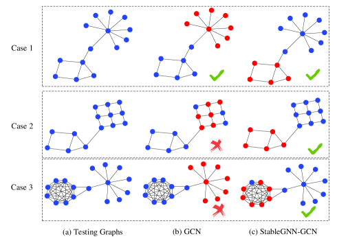
Figure 5: Explanation cases of GCN and StableGNN-GCN. Red nodes are the important subgraph calculated by the GNNExplainer.

5.2 Experiments on Real-world Datasets

In this section, we apply our StableGNN algorithm on eight real-world datasets for out-of-distribution graph property prediction.

Datasets. We adopt seven molecular property prediction datasets from OGB Datasets (Hu et al., 2020). All the molecules are pre-processed using RDKit (Landrum et al., 2006). Each graph represents a molecule, where nodes are atoms, and edges are chemical bonds. We use the 9-dimensional node features and 3-dimensional edges features provided by  (Hu et al., 2020), which has better generalization performance. The task of these datasets is to predict the target molecular properties, e.g., whether a molecule inhibits HIV virus replication or not. Input edge features are 3-dimensional, containing bond type, bond stereochemistry as well as an additional bond feature indicating whether the bond is conjugated. Depending on the properties of molecular, these datasets can be categorized into three kinds of tasks: binary classification, multi-label classification and regression. Different from commonly used random splitting, these datasets adopt scaffold splitting (Wu et al., 2018) procedure that splits the molecules based on their two-dimensional structural frameworks. The scaffold splitting attempts to separate structurally different molecules into different subsets, which provides a more realistic estimate of model performance in prospective experimental settings. Due to the selection bias of training set, it will inevitably introduce the spurious correlation between the subgraphs of molecules. Moreover, we also conduct the experiments on a commonly used graph classification dataset, MUTAG (Debnath et al., 1991), as we could explain the results based on the knowledge used in (Luo et al., 2020). It consists of 4,337 molecule graphs. Each graph is assigned to one of 2 classes based on its mutagenic effect. Note that this dataset cannot adopt the scaffold splitting, as the +4 valence N atom, which commonly exists in this dataset, is illegal in the RDKit (Landrum, 2013) tool used for scaffold splitting. We just use the random splitting for this dataset, however, we still believe there are some OOD cases in the testing set. The splitting ratio for all the datasets is 80/10/10. The detailed statistics are shown in Table 2.

Baselines. As the superiority of GNNs against traditional method on graph-level task, like kernel-based methods (Shervashidze et al., 2011; 2009), has been demonstrated by previous literature (Ying et al., 2018), here, we mainly consider baselines based upon several related and state-of-the-art GNNs.

• Base models: GraphSAGE (Hamilton et al., 2017) and GCN (Kipf & Welling, 2016) are classical GNN methods. We utilize them as base models in our framework, so they are the most related baselines to validate the effectiveness the proposed framework.

• DIFFPOOL (Ying et al., 2018): It is a hierarchical graph pooling method in an end-to-end fashion. It adopts the same model architecture and hyperparamter setting with high-level variable learning component in our framework, except that DIFFPOOL model aggregates the clusters’ representation by summation operation rather than an ordered concatenation operation to generate the final high-level representations.

• GAT (Veličković et al., 2017): It is an attention-based GNN method, which learns the edge weights by an attention mechanism.

• GIN (Xu et al., 2019): It is a graph isomorphism network that is as powerful as the WL graph isomorphism test. We compare with two variants of GIN, i.e., whether the $\epsilon$ is a learnable parameter or a fixed 0 scalar, denoted as GIN and GIN0, respectively.

• MoNet (Monti et al., 2017): It is a general architecure to learn on graphs and manifolds using the bayesian gaussian mixture model.

• SGC (Wu et al., 2019): It is a simplified GCN-based method, which reduces the excess complexity through successively removing nonlinearities and collapsing weight matrices between consecutive layers.

• JKNet (Xu et al., 2018): It is a GNN framework that selectively combines different aggregations at the last layer.

Experimental Settings and Metrics. Here, we only describe the experimental settings that is different from Section 5.1. For all the GNN baselines, the number of layers is set as 5. The dropout rate after each layer for all the methods on the datasets for binary classification and multi-label classification is set as 0.5, and for regression datasets, the dropout rate is set as 0.0. The number of batch size for binary classification and multi-label classification is set as 128, and for regression datasets, the batch size is set as 64. The training epoch for all the baselines is set as 200. And for our model, we utilize 100 epoch to warm up and 100 epoch to train the whole model. The number of clusters is set as 7 for our models and DIFFPOOL. As these datasets usually treat chemical bond type as their edge type, to include edge features, we follow (Hu et al., 2020) and add transformed edge features into the incoming node features. For the datasets from OGB, we use the metrics recommended by original paper for each task (Hu et al., 2020). And following (Ying et al., 2019), we adopt Accuracy for MUTAG dataset.

Table 2: Summary of real-world datasets.

Dataset	Task Type	#Graphs	Average #Nodes	Average #Edges	#Task	Splitting Type	Metric
Molbace	Binary classification	1,513	34.1	36.9	1	Scaffold splitting	ROC-AUC
Molbbbp	Binary classification	2,039	24.1	26.0	1	Scaffold splitting	ROC-AUC
Molhiv	Binary classification	41,127	25.5	27.5	1	Scaffold splitting	ROC-AUC
MUTAG	Binary classification	4,337	30.32	30.77	1	Random splitting	Accuracy
Molclintox	Multi-label classification	1,477	26.2	27.9	2	Scaffold splitting	ROC-AUC
Moltox21	Multi-label classification	7,831	18.6	19.3	12	Scaffold splitting	ROC-AUC
Molesol	Regression	1,128	13.3	13.7	1	Scaffold splitting	RMSE
Mollipo	Regression	4,200	27.0	29.5	1	Scaffold splitting	RMSE

Results on Real-world Datasets. The experimental results on eight datasets are presented in Table 3, and we have the following observations. First, comparing with these competitive GNN models, StableGNN-SAGE/GCN achieves 6 first places and 2 second places on all eight datasets. And the average rank of StableGNN-SAGE and StableGNN-GCN are 1.75 and 2.87, respectively, which is much higher than the third place, i.e., 4.38 for MoNet. It means that most existing GNN models cannot perform well on OOD datasets and our model significantly outperforms existing methods, which well demonstrates the effectiveness of the proposed causal representation learning framework. Second, comparing with the base models, i.e., GraphSAGE and GCN, our models achieve consistent improvements on all datasets, validating that our framework could boost the existing GNN architectures. Third, StableGNN-SAGE/GCN also outperforms DIFFPOOL method with a large margin. Although we utilize the DiffPool layer to extract high-level representations in our framework, the seamless integration of representation learning and causal learning is the key to the improvements of our model. Fourth, StableGNN-SAGE/GCN achieves superior performance on datasets with three different tasks and a wide range of dataset scales, indicating that our proposed framework is general enough to adopt datasets with a variety of properties.

Table 3: Performance of real-world graph datasets. The number in the $(\cdot)$ along with each performance number means the rank of the method among all the methods on this dataset. “$\uparrow$” means that for this metric, the larger value means better performance. “$\downarrow$” means that for this metric, the smaller value means better performance. Best results of all methods are indicated in bold.

Methods	Binary Classification
	Molhiv	Molbace	Molbbbp	MUTAG
	ROC-AUC ($\uparrow$)	ROC-AUC ($\uparrow$)	ROC-AUC ($\uparrow$)	Accuracy ($\uparrow$)
GIN	76.21$\pm$0.53 (6)	74.50$\pm$2.75 (9)	67.72$\pm$1.89 (4)	78.86$\pm$1.15 (10)
GIN0	75.49$\pm$0.91 (9)	74.36$\pm$3.48 (10)	66.65$\pm$1.32 (6)	79.03$\pm$0.56 (9)
GAT	76.52$\pm$0.69 (5)	81.17$\pm$0.8 (1)	67.17$\pm$0.49 (5)	79.26$\pm$1.13 (8)
MoNet	77.13$\pm$0.79 (3)	76.92$\pm$0.91 (6)	69.52$\pm$0.46 (1)	79.95$\pm$0.86 (4)
SGC	69.46$\pm$1.44 (11)	71.28$\pm$1.79 (11)	61.17$\pm$2.91 (11)	69.53$\pm$0.77 (11)
JKNet	74.99$\pm$1.60 (10)	78.99$\pm$13.4 (3)	65.62$\pm$0.77 (9)	79.49$\pm$1.16 (7)
DIFFPOOL	75.75$\pm$1.38 (8)	74.69$\pm$11.13 (8)	63.35$\pm$2.21 (10)	80.13$\pm$1.32 (3)
GCN	76.63$\pm$1.13 (4)	75.88$\pm$1.85 (7)	66.47$\pm$0.90 (7)	79.89$\pm$1.32 (5)
StableGNN-GCN	77.79 $\pm$1.19 (1)	76.95$\pm$3.27 (5)	68.82$\pm$3.87 (2)	81.45$\pm$2.00 (2)
GraphSAGE	75.78$\pm$2.19 (6)	78.51$\pm$1.72 (4)	66.16$\pm$0.97 (8)	79.78$\pm$0.78 (6)
StableGNN-SAGE	77.63$\pm$0.79 (2)	80.73$\pm$3.98 (2)	68.47$\pm$2.47 (3)	82.13$\pm$0.32 (1)
Methods	Multilabel Classification		Regression		Average-Rank
	Molclintox	Moltox21	Molesol	Molipo
	ROC-AUC ($\uparrow$)	ROC-AUC ($\uparrow$)	RMSE ($\downarrow$)	RMSE ($\downarrow$)	($\downarrow$)
GIN	86.86$\pm$3.78 (6)	64.20$\pm$0.23 (11)	1.1002$\pm$0.0450 (4)	0.8051$\pm$0.0323 (10)	7.50 (9)
GIN0	89.31$\pm$2.11 (3)	64.62$\pm$0.87 (10)	1.1358$\pm$0.0587 (5)	0.8050$\pm$0.0123 (9)	7.63 (10)
GAT	83.47$\pm$1.37 (8)	68.81$\pm$0.48 (5)	1.2758$\pm$0.0269 (10)	0.8101$\pm$0.0183 (9)	6.38 (7)
MoNet	86.75$\pm$1.22 (7)	67.02$\pm$0.26 (7)	1.0753$\pm$0.0357 (3)	0.7379$\pm$0.0117 (4)	4.38 (3)
SGC	77.76$\pm$1.87 (10)	66.49$\pm$1.10 (8)	1.6548$\pm$0.0462 (11)	1.0681$\pm$0.0148 (10)	10.38 (11)
JKNet	81.63$\pm$2.79 (9)	65.98$\pm$0.46 (9)	1.1688$\pm$0.0434 (7)	0.7493$\pm$0.0048 (5)	7.38 (8)
DIFFPOOL	90.48$\pm$2.42 (2)	69.05$\pm$0.94 (3)	1.176$\pm$0.01388 (8)	0.7325$\pm$0.0221 (2)	5.50 (4)
GCN	86.23$\pm$2.81 (7)	67.75$\pm$0.66 (6)	1.153$\pm$0.0392 (6)	0.7927$\pm$0.0086 (8)	6.25 (6)
StableGNN-GCN	87.98$\pm$2.37 (5)	70.80$\pm$0.31 (1)	0.9638$\pm$0.0292 (1)	0.7839$\pm$0.0165 (6)	2.87 (2)
GraphSAGE	88.60$\pm$2.44 (4)	68.88$\pm$0.59 (4)	1.1852$\pm$0.0353 (9)	0.7911$\pm$0.0147 (7)	6.00 (5)
StableGNN-SAGE	90.96$\pm$1.93 (1)	69.14$\pm$0.24 (2)	1.0092$\pm$0.0706 (2)	0.6971$\pm$0.0297 (1)	1.75 (1)

Ablation Study. Note that our framework naturally fuses the high-level representation learning and causal effect estimation in a unified framework. Here we conduct ablation studies to investigate the effect of each component. For our framework without the CVD regularizer, we term it as StableGNN-NoCVD. The results are presented in Figure 6. We first find that StableGNN-NoCVD outperforms GraphSAGE on most datasets, indicating that learning hierarchical structure by our model for graph-level task is necessary and effective. Second, StableGNN-NoCVD achieves competitive results or better results with DIFFPOOL method. The only difference between them is that DIFFPOOL model averages the learned clusters’ representations and StableGNN-NoCVD concatenates them by a consistent order, and then the aggregated embeddings are fed into a classifier. As the traditional MLP classifier needs the features of all samples should in a consistent order, the superior performance of StableGNN-NoCVD well validates that the learned representations $\mathbf{H}$ are in a consistent order across graphs. Moreover, we find that StableGNN consistently outperforms StableGNN-NoCVD. As the only difference between the two models is the CVD term, we can safely attribute the improvements to the distinguishing of causal variables by our proposed regularizer. Note that on some datasets, we could find that StableGNN-NoDVD cannot achieve satisfying results, however, when combining with the regularizer, it makes clear improvements. This phenomenon further validates the necessity of each component that we should conduct representation learning and causal inference jointly.

(a) Binary Classification ($\uparrow$)

(b) Multilabel Classification ($\uparrow$)

(c) Regression ($\downarrow$)

Figure 6: Ablation study on three real-world tasks.

Comparison with Different Decorrelation Methods. As there may be other ways to decorrelate the variables in GNNs by sample reweighting methods, one question arises naturally: is our proposed decorrelation framework a more suitable strategy for graphs? To answer this question, we compare the following alternatives:

• GraphSAGE-Decorr: This method directly decorrelates each dimension of graph-level representations learned by GraphSAGE.

• StableGNN-NoCVD-Decorr: This method decorrelates each dimension of concatenated high-level representation $\mathbf{H}$ learned by StableGNN-NoCVD.

• StableGNN-NoCVD-Distent: This method forces the high-level representation learned by StableGNN-NoCVD to be disentangled via adding a HSIC regularizer to the overall loss.

The results are shown in Table 4. Comparing with these potential decorrelation methods, StableGNN achieves better results consistently, demonstrating that decorrelating the representations by the cluster-level granularity is a more suitable strategy for graph data. Moreover, we find that GraphSAGE-Decorr/StableGNN-NoCVD-Decorr shows worse performance than GraphSAGE/StableGNN-NoCVD, and the reason is that if we aggressively decorrelate single dimension of embeddings, it will inevitably break the intrinsic semantic meaning of original data. Furthermore, StableGNN-NoCVD-Distent forces the high-level representations to be disentangled, which changes the semantic implication of features, while StableGNN learns sample weights to adjust the data structure while the semantic of features is not effected. Overall, StableGNN is a general and effective framework comparing with all the potential ways.

Table 4: Performance of different decorrelation methods.

Method	Molhiv	Molbace	Molbbbp	MUTAG	Molclintox	Moltox21	Molesol	Mollipo
GraphSAGE	75.78$\pm$2.19	78.51$\pm$1.72	66.16$\pm$0.97	79.78$\pm$0.7	88.60$\pm$2.44	68.88$\pm$0.59	1.8098$\pm$0.1220	0.7911$\pm$0.0147
GraphSAGE-Decorr	76.52$\pm$0.69	77.34$\pm$5.63	66.28$\pm$0.89	80.76$\pm$1.32	86.51$\pm$0.82	68.77$\pm$0.66	1.7889$\pm$0.1234	0.8024$\pm$0.0165
StableGNN-NoCVD	76.47$\pm$1.01	79.65$\pm$0.86	66.73$\pm$1.87	80.13$\pm$1.80	87.56$\pm$1.91	68.63$\pm$0.63	1.0819$\pm$0.0219	0.6971$\pm$0.017
StableGNN-NoCVD-Decorr	75.32$\pm$0.52	78.71$\pm$2.34	67.02$\pm$1.55	79.17$\pm$1.07	88.89$\pm$2.58	69.05$\pm$0.66	1.0377$\pm$0.0389	0.7171$\pm$0.0378
StableGNN-NoCVD-Distent	75.76$\pm$0.64	79.04$\pm$1.24	64.21$\pm$1.34	80.92+0.50	90.44$\pm$0.79	68.87$\pm$1.28	1.0729$\pm$0.0256	0.7171$\pm$0.0378
StableGNN	77.63$\pm$0.79	80.73$\pm$3.98	68.47$\pm$2.47	82.13$\pm$0.32	90.96$\pm$1.93	69.14$\pm$0.24	1.022$\pm$0.0039	0.6971$\pm$0.0297

Convergence Rate and Parameter Sensitivity Analysis. We first analyze the convergence rate of our proposed causal variable distinguishing regularizer. We report the summation of HSIC value of all high-level representation pairs and the difference of learned weights between two consecutive epochs during the weights learning procedure in one batch on three relatively smaller datasets in Figure 7. As we can see, the weights learned by CVD regularizer could achieve convergence very fast while reducing the HSIC value significantly. In addition, we study the sensitivity of the number of high-level representations and report the performance of StableGNN-NoCVD and StableGNN based on the same pre-defined number of clusters in Figure 8. StableGNN outperforms StableGNN-NoCVD on almost all cases, which well demonstrates the robustness of our methods with the number of pre-defined clusters and the effectiveness of the proposed CVD regularizer. Note that our framework could learn the appropriate number of clusters in an end-to-end way, i.e., some clusters might not be used by the assignment matrix.

(a) Molbace

(b) Molbbbp

(c) Molclintox

Figure 7: Convergence rate analysis of CVD regularizer.

(a) Molbace($\uparrow$)

(b) Molbbbp($\uparrow$)

(c) Molclintox($\uparrow$)

Figure 8: Sensitivity of the pre-defined maximum number of clusters.

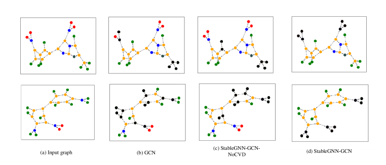
Figure 9: Explanation instance for MUTAG dataset. The blue, green, red and yellow color represent N, H, O, C atom, respectively. The top important subgraphs selected by GNNExplainer are viewed in black color (keep top 6 important edges). The picture is best viewed in color.

Interpretability Analysis. In Figure 9, we investigate explanations for graph classification task on MUTAG dataset. In the MUTAG example, colors indicate node features, which represent atoms. StableGNN correctly identifies chemical $NO_{2}$ and $NH_{2}$, which are known to be mutagenic (Luo et al., 2020) while baselines fail in. These cases demonstrate that our model could utilize more interpretable structures for prediction. Moreover, the difference of StableGNN-GCN-NoCVD between StableGNN-GCN indicates the necessity of integrating two components in our framework.

6 Conclusion and Further work

In this paper, we study a practical but seldom studied problem: generalizing GNNs on out-of-distribution graph data. We analyze the problem in a causal view that the generalization of GNNs will be hindered by the spurious correlation among subgraphs. To improve the stability of existing methods, we propose a general causal representation learning framework, called StableGNN, which integrates graph high-level variable representation learning and causal effect estimation in a unified framework. Extensive experiments well demonstrate the effectiveness, flexibility, and interpretability of the StableGNN.

In addition, we believe that this paper just opens a direction for causal representation learning on graphs. As the most important contribution, we propose a general framework for causal graph representation learning: graph high-level variable representation learning and causal variable distinguishing, which can be flexibly adjusted for specific tasks. For example, a multi-channel filter may be adopted to learn different signals on graphs into subspaces. And for some datasets there may exist more complicated causal relationships among high-level variables, hence discovering causal structure for these high-level variables may be useful for reconstructing original data generation process. To be border impact, we believe the idea could also spur the causal representation learning in other areas, like object recognition and automatic driving in wild environments.

References

- Angrist & Imbens (1995) Joshua Angrist and Guido Imbens. Identification and estimation of local average treatment effects, 1995.
- Arjovsky et al. (2019) Martin Arjovsky, Léon Bottou, Ishaan Gulrajani, and David Lopez-Paz. Invariant risk minimization. arXiv preprint arXiv:1907.02893, 2019.
- Athey et al. (2016) Susan Athey, Guido W Imbens, and Stefan Wager. Approximate residual balancing: De-biased inference of average treatment effects in high dimensions. arXiv preprint arXiv:1604.07125, 2016.
- Bengio et al. (2019) Yoshua Bengio, Tristan Deleu, Nasim Rahaman, Rosemary Ke, Sébastien Lachapelle, Olexa Bilaniuk, Anirudh Goyal, and Christopher Pal. A meta-transfer objective for learning to disentangle causal mechanisms. arXiv preprint arXiv:1901.10912, 2019.
- Bo et al. (2021) Deyu Bo, Xiao Wang, Chuan Shi, and Huawei Shen. Beyond low-frequency information in graph convolutional networks. 2021.
- Debnath et al. (1991) Asim Kumar Debnath, Rosa L Lopez de Compadre, Gargi Debnath, Alan J Shusterman, and Corwin Hansch. Structure-activity relationship of mutagenic aromatic and heteroaromatic nitro compounds. correlation with molecular orbital energies and hydrophobicity. Journal of medicinal chemistry, 34(2):786–797, 1991.
- Engstrom et al. (2019) Logan Engstrom, Brandon Tran, Dimitris Tsipras, Ludwig Schmidt, and Aleksander Madry. Exploring the landscape of spatial robustness. In ICML, pp. 1802–1811. PMLR, 2019.
- Gao & Ji (2019) Hongyang Gao and Shuiwang Ji. Graph u-nets. In international conference on machine learning, pp. 2083–2092. PMLR, 2019.
- Gilmer et al. (2017) Justin Gilmer, Samuel S Schoenholz, Patrick F Riley, Oriol Vinyals, and George E Dahl. Neural message passing for quantum chemistry. In ICML, pp. 1263–1272. PMLR, 2017.
- Gretton et al. (2005) Arthur Gretton, Olivier Bousquet, Alex Smola, and Bernhard Schölkopf. Measuring statistical dependence with hilbert-schmidt norms. In International conference on algorithmic learning theory, pp. 63–77. Springer, 2005.
- Hainmueller (2012) Jens Hainmueller. Entropy balancing for causal effects: A multivariate reweighting method to produce balanced samples in observational studies. Political Analysis, 20(1):25–46, 2012.
- Hamilton et al. (2017) Will Hamilton, Zhitao Ying, and Jure Leskovec. Inductive representation learning on large graphs. In NeurIPS, pp. 1024–1034, 2017.
- He et al. (2016) Kaiming He, Xiangyu Zhang, Shaoqing Ren, and Jian Sun. Deep residual learning for image recognition. In Proceedings of the IEEE conference on computer vision and pattern recognition, pp. 770–778, 2016.
- Hendrycks & Dietterich (2019) Dan Hendrycks and Thomas Dietterich. Benchmarking neural network robustness to common corruptions and perturbations. arXiv preprint arXiv:1903.12261, 2019.
- Hu et al. (2020) Weihua Hu, Matthias Fey, Marinka Zitnik, Yuxiao Dong, Hongyu Ren, Bowen Liu, Michele Catasta, and Jure Leskovec. Open graph benchmark: Datasets for machine learning on graphs. 2020.
- Huang & Ling (2005) Jin Huang and Charles X Ling. Using auc and accuracy in evaluating learning algorithms. TKDE, 17(3):299–310, 2005.
- (17) Sergey Ioffe and Christian Szegedy Batch Normalization. Accelerating deep network training by reducing internal covariate shift. arXiv preprint arXiv:1502.03167.
- Jin et al. (2020) Wengong Jin, Regina Barzilay, and Tommi Jaakkola. Hierarchical generation of molecular graphs using structural motifs. In ICML, pp. 4839–4848. PMLR, 2020.
- Kamath et al. (2021) Pritish Kamath, Akilesh Tangella, Danica Sutherland, and Nathan Srebro. Does invariant risk minimization capture invariance? In International Conference on Artificial Intelligence and Statistics, pp. 4069–4077. PMLR, 2021.
- Keriven & Peyré (2019) Nicolas Keriven and Gabriel Peyré. Universal invariant and equivariant graph neural networks. NeurIPS, 32:7092–7101, 2019.
- Kipf & Welling (2016) Thomas N Kipf and Max Welling. Semi-supervised classification with graph convolutional networks. In ICLR, 2016.
- Krueger et al. (2021) David Krueger, Ethan Caballero, Joern-Henrik Jacobsen, Amy Zhang, Jonathan Binas, Dinghuai Zhang, Remi Le Priol, and Aaron Courville. Out-of-distribution generalization via risk extrapolation (rex). In ICML, pp. 5815–5826, 2021.
- Kuang et al. (2018) Kun Kuang, Peng Cui, Susan Athey, Ruoxuan Xiong, and Bo Li. Stable prediction across unknown environments. In KDD, pp. 1617–1626, 2018.
- Kuang et al. (2020) Kun Kuang, Ruoxuan Xiong, Peng Cui, Susan Athey, and Bo Li. Stable prediction with model misspecification and agnostic distribution shift. In AAAI, 2020.
- Lake et al. (2017) Brenden M Lake, Tomer D Ullman, Joshua B Tenenbaum, and Samuel J Gershman. Building machines that learn and think like people. Behavioral and brain sciences, 40, 2017.
- Landrum (2013) Greg Landrum. Rdkit: A software suite for cheminformatics, computational chemistry, and predictive modeling, 2013.
- Landrum et al. (2006) Greg Landrum et al. Rdkit: Open-source cheminformatics. 2006.
- Lee et al. (2018) John Boaz Lee, Ryan Rossi, and Xiangnan Kong. Graph classification using structural attention. In SIGKDD, pp. 1666–1674, 2018.
- Lee et al. (2019) Junhyun Lee, Inyeop Lee, and Jaewoo Kang. Self-attention graph pooling. In ICML, pp. 3734–3743. PMLR, 2019.
- Leman & Weisfeiler (1968) AA Leman and B Weisfeiler. A reduction of a graph to a canonical form and an algebra arising during this reduction. Nauchno-Technicheskaya Informatsiya, 2(9):12–16, 1968.
- Liao et al. (2020) Renjie Liao, Raquel Urtasun, and Richard Zemel. A pac-bayesian approach to generalization bounds for graph neural networks. 2020.
- Lin et al. (2021) Wanyu Lin, Hao Lan, and Baochun Li. Generative causal explanations for graph neural networks. In ICML, 2021.
- Lopez-Paz et al. (2017) David Lopez-Paz, Robert Nishihara, Soumith Chintala, Bernhard Scholkopf, and Léon Bottou. Discovering causal signals in images. In CVPR, pp. 6979–6987, 2017.
- Luo et al. (2020) Dongsheng Luo, Wei Cheng, Dongkuan Xu, Wenchao Yu, Bo Zong, Haifeng Chen, and Xiang Zhang. Parameterized explainer for graph neural network. In NeurIPS, 2020.
- Matsuura & Harada (2020) Toshihiko Matsuura and Tatsuya Harada. Domain generalization using a mixture of multiple latent domains. In AAAI, volume 34, pp. 11749–11756, 2020.
- Monti et al. (2017) Federico Monti, Davide Boscaini, Jonathan Masci, Emanuele Rodola, Jan Svoboda, and Michael M Bronstein. Geometric deep learning on graphs and manifolds using mixture model cnns. In CVPR, pp. 5115–5124, 2017.
- Pope et al. (2019) Phillip E Pope, Soheil Kolouri, Mohammad Rostami, Charles E Martin, and Heiko Hoffmann. Explainability methods for graph convolutional neural networks. In CVPR, pp. 10772–10781, 2019.
- Qiao et al. (2020) Fengchun Qiao, Long Zhao, and Xi Peng. Learning to learn single domain generalization. In CVPR, pp. 12556–12565, 2020.
- Rosenfeld et al. (2020) Elan Rosenfeld, Pradeep Ravikumar, and Andrej Risteski. The risks of invariant risk minimization. 2020.
- Scarselli et al. (2008) Franco Scarselli, Marco Gori, Ah Chung Tsoi, Markus Hagenbuchner, and Gabriele Monfardini. The graph neural network model. IEEE Transactions on Neural Networks, 20(1):61–80, 2008.
- Schlichtkrull et al. (2018) Michael Schlichtkrull, Thomas N Kipf, Peter Bloem, Rianne Van Den Berg, Ivan Titov, and Max Welling. Modeling relational data with graph convolutional networks. In European semantic web conference, pp. 593–607. Springer, 2018.
- Schölkopf et al. (2021) Bernhard Schölkopf, Francesco Locatello, Stefan Bauer, Nan Rosemary Ke, Nal Kalchbrenner, Anirudh Goyal, and Yoshua Bengio. Toward causal representation learning. Proceedings of the IEEE, 109(5):612–634, 2021.
- Shen et al. (2018) Zheyan Shen, Peng Cui, Kun Kuang, Bo Li, and Peixuan Chen. Causally regularized learning with agnostic data selection bias. In MM, pp. 411–419, 2018.
- Shen et al. (2020) Zheyan Shen, Peng Cui, Tong Zhang, and Kun Kuang. Stable learning via sample reweighting. In AAAI, pp. 5692–5699, 2020.
- Shervashidze et al. (2009) Nino Shervashidze, SVN Vishwanathan, Tobias Petri, Kurt Mehlhorn, and Karsten Borgwardt. Efficient graphlet kernels for large graph comparison. In Artificial intelligence and statistics, pp. 488–495. PMLR, 2009.
- Shervashidze et al. (2011) Nino Shervashidze, Pascal Schweitzer, Erik Jan Van Leeuwen, Kurt Mehlhorn, and Karsten M Borgwardt. Weisfeiler-lehman graph kernels. Journal of Machine Learning Research, 12(9), 2011.
- Song et al. (2007) Le Song, Alex Smola, Arthur Gretton, Karsten M Borgwardt, and Justin Bedo. Supervised feature selection via dependence estimation. In ICML, pp. 823–830, 2007.
- Song et al. (2012) Le Song, Alex Smola, Arthur Gretton, Justin Bedo, and Karsten Borgwardt. Feature selection via dependence maximization. Journal of Machine Learning Research, 13(5), 2012.
- Su et al. (2019) Jiawei Su, Danilo Vasconcellos Vargas, and Kouichi Sakurai. One pixel attack for fooling deep neural networks. TEC, 23(5):828–841, 2019.
- Sun et al. (2019) Yu Sun, Xiaolong Wang, Zhuang Liu, John Miller, Alexei A Efros, and Moritz Hardt. Test-time training for out-of-distribution generalization. 2019.
- Veličković et al. (2017) Petar Veličković, Guillem Cucurull, Arantxa Casanova, Adriana Romero, Pietro Lio, and Yoshua Bengio. Graph attention networks. In ICLR, 2017.
- Wang et al. (2019) Haohan Wang, Zexue He, Zachary C Lipton, and Eric P Xing. Learning robust representations by projecting superficial statistics out. arXiv preprint arXiv:1903.06256, 2019.
- Wu et al. (2019) Felix Wu, Amauri Souza, Tianyi Zhang, Christopher Fifty, Tao Yu, and Kilian Weinberger. Simplifying graph convolutional networks. In ICML, pp. 6861–6871. PMLR, 2019.
- Wu et al. (2018) Zhenqin Wu, Bharath Ramsundar, Evan N Feinberg, Joseph Gomes, Caleb Geniesse, Aneesh S Pappu, Karl Leswing, and Vijay Pande. Moleculenet: a benchmark for molecular machine learning. Chemical science, 9(2):513–530, 2018.
- Xu et al. (2018) Keyulu Xu, Chengtao Li, Yonglong Tian, Tomohiro Sonobe, Ken-ichi Kawarabayashi, and Stefanie Jegelka. Representation learning on graphs with jumping knowledge networks. In ICML, pp. 5453–5462. PMLR, 2018.
- Xu et al. (2019) Keyulu Xu, Weihua Hu, Jure Leskovec, and Stefanie Jegelka. How powerful are graph neural networks? In ICLR, 2019. URL https://openreview.net/forum?id=ryGs6iA5Km.
- Ying et al. (2018) Rex Ying, Jiaxuan You, Christopher Morris, Xiang Ren, William L Hamilton, and Jure Leskovec. Hierarchical graph representation learning with differentiable pooling. In NeurIPS, 2018.
- Ying et al. (2019) Rex Ying, Dylan Bourgeois, Jiaxuan You, Marinka Zitnik, and Jure Leskovec. Gnnexplainer: Generating explanations for graph neural networks. In NeurIPS, 2019.
- Zhang & Chen (2018) Muhan Zhang and Yixin Chen. Link prediction based on graph neural networks. volume 31, pp. 5165–5175, 2018.
- Zhang et al. (2018) Muhan Zhang, Zhicheng Cui, Marion Neumann, and Yixin Chen. An end-to-end deep learning architecture for graph classification. In AAAI, 2018.
- Zhang et al. (2021) Xingxuan Zhang, Peng Cui, Renzhe Xu, Linjun Zhou, Yue He, and Zheyan Shen. Deep stable learning for out-of-distribution generalization. In CVPR, pp. 5372–5382, 2021.
- Zou et al. (2020) Hao Zou, Peng Cui, Bo Li, Zheyan Shen, Jianxin Ma, Hongxia Yang, and Yue He. Counterfactual prediction for bundle treatment. NeurIPS, 33, 2020.
- Zubizarreta (2015) José R Zubizarreta. Stable weights that balance covariates for estimation with incomplete outcome data. Journal of the American Statistical Association, 110(511):910–922, 2015.