Absorption and optical selection rules of tunable excitons in biased bilayer graphene

Abstract

Biased bilayer graphene, with its easily tunable band gap, presents itself as the ideal system to explore the excitonic effect in graphene based systems. In this paper we study the excitonic optical response of such a system by combining a tight binding model with the solution of the Bethe-Salpeter equation, the latter being solved in a semi-analytical manner, requiring a single numerical quadrature, thus allowing for a transparent calculation. With our approach we start by analytically obtaining the optical selection rules, followed by the computation of the absorption spectrum for the case of a biased bilayer encapsulated in hexagonal boron nitride, a system which has been the subject of a recent experimental study. An excellent agreement is seen when we compare our theoretical prediction with the experimental data.

I Introduction

Since graphene was first isolated [1] many other two dimensional materials have be discovered. Examples of these are the semiconductor monolayer transition metal dichalcogenides (TMDs) [2], the highly anisotropic phosphorene [3], or the insulator hexagonal boron nitride (hBN) [4]. Despite their own unique properties, these three materials have something in common, all of them have an optical response dominated by excitonic effects.

In the simplest possible picture, an exciton is formed upon the excitation of an electron to the conduction band, leaving a hole in the valence band. These two particles, which have opposite charges, interact via an electrostatic potential [5]. This situation is somewhat similar to what is found in the Hydrogen atom, and leads to the formation of bound states inside the band gap of the material. Due to the reduced screening in the out-of-plane direction, two dimensional materials host excitons with large binding energies , easily surpassing the energies usually found in their three dimensional counterparts. Furthermore, excitons in these 2D systems couple efficiently with light resulting in huge oscillator strengths. This has made the exploration of excitonic effects a rich research field, with many possible applications, such as deep-UV optoelectronics [6, 7, 4] in hBN, or the exploration of valleytronics [8] and single photon emitters [9, 10] in TMDs, which are of great importance in the field of quantum information. Furthermore, it has been recently shown that the combination of a TMD with a Van der Waals heterostructure cavity enhances the light-mater interaction, thus allowing for unitary excitonic absorption [11].

Although present in many 2D materials, low energy excitonic bound states are noticeably absent in pristine monolayer graphene, something easily understood if one recalls that this material is a semi-metal, thus lacking the necessary band gap for the formation of such states. This, however, does not stop us from studying excitonic physics in graphene based systems, since through material engineering many systems can be designed to obtain the desired properties. A clear example of this is the case of biased bilayer graphene (BBLG), where two graphene monolayers are stacked and a displacement field is applied to them. Even though bilayer graphene (BLG) inherits the lack of a band gap from its monolayer form, the presence of the displacement field opens a gap in the system, which can be finely tuned from the mid to far-infrared [12, 13, 14]. This finite gap is the key ingredient to combine the desirable properties of excitons with the unique physics of graphene based systems.

The first theoretical study about excitons in BBLG was carried out in Ref. [15], where a pronounced resonance, sensitive to the displacement field, was predicted to appear inside the band gap in absorption measurements. More recently, in Ref. [16], an experimental study was carried out to characterize the excitonic optical response of BBLG encapsulated in hBN. Our goal with this paper is to produce a theoretical description of the experimental data measured in that work. To achieve this, we will describe the electronic properties using a tight binding model, while solving the Bethe-Salpeter equation (BSE) to obtain the energies and wave functions of the excitons. While oftentimes the BSE is coupled to DFT calculations , and solved in a fully numerical manner [15, 17, 18, 19, 20], requiring huge computational effort, our approach uses a simple analytical treatment which requires a single numerical quadrature, thus greatly reducing the numerical cost of the computation.

This paper is organized as follows. In Sec. II we introduce the tight binding model which describes the biased bilayer, and diagonalize it. In Sec. III, we start the discussion on the excitonic properties of the system, which we obtain by solving the Bethe-Salpeter equation. In Sec. IV, we discuss the optical properties of the biased bilayer. First, we discuss the optical selection rules; then we compute the absorption spectrum and compare it with the experimental results of Ref. [16]. Finally, in Sec. V, we give an overview of the paper and our closing remarks. An appendix describing how to efficiently solve the Bethe-Salpeter equation closes the paper.

II Tight binding model

To start our discussion let us study the electronic properties of a graphene bilayer subject to an external bias, which we schematically depict in Figure 1.

Figure 1: (a) Top view of Bernal stacked bilayer graphene. The atoms of different sub-lattices are colored in different tones for clarity. Also depicted is the intralayer nearest neighbor hopping $\gamma_{0}$. (b) Side view of the bilayer graphene. (c)-(f) Schematic representation of nearest neighbor and next nearest neighbor interlayer hoppings.

To characterize this system we shall employ a tight binding Hamiltonian written directly in momentum space. To obtain this Hamiltonian we account for nearest neighbors intralayer hoppings ($\gamma_{0}$), as well as nearest neighbors $(\gamma_{1})$ and next nearest neighbors ($\gamma_{3}$, $\gamma_{4}$ and $\gamma_{5}$) interlayer hoppings. Doing so, one finds the Hamiltonian to be:

$$H_{\textrm{TB}}=\left[\begin{array}[]{cccc}V&\gamma_{0}\phi(\mathbf{k})&\gamma_{1}&\gamma_{4}\phi^{*}(\mathbf{k})\\ \gamma_{0}\phi^{*}(\mathbf{k})&V&\gamma_{3}\phi^{*}(\mathbf{k})&\gamma_{5}\phi(\mathbf{k})\\ \gamma_{1}&\gamma_{3}\phi(\mathbf{k})&-V&\gamma_{0}\phi^{*}(\mathbf{k})\\ \gamma_{4}\phi(\mathbf{k})&\gamma_{5}\phi^{*}(\mathbf{k})&\gamma_{0}\phi(\mathbf{k})&-V\end{array}\right],$$ (1)

when written in the basis $\{|1,b\rangle,|2,b\rangle,|1,t\rangle,|2,t\rangle\}$ (with $b$ and $t$ denoting the bottom and top layers, respectively, and the labels $1$ and $2$ are defined as in Fig. 1). Here, $V$ quantifies the bias and $\phi(\mathbf{k})=e^{iak_{y}}+e^{ia(k_{x}\sqrt{3}-k_{y})/2}+e^{-ia(k_{x}\sqrt{3}+k_{y})/2}$ is a phase factor determined by the honeycomb geometry of the individual layers. Since we will be mostly interested in the low energy response of the system, we shall restrict our study to the vicinity of the Dirac points of the the first Brillouin zone. Mathematically, this amounts to approximating the phase factor $\phi(\mathbf{k})$ as $\phi(\mathbf{k})\approx\frac{3}{2}a(\tau k_{x}+ik_{y})$, with $\tau=\pm 1$ labeling the two Dirac points. Note that henceforth, the momentum $\mathbf{k}=(k_{x},k_{y})$ is measured relatively to the chosen Dirac point. With this approximation one finds the low energy Hamiltonian

$$\frac{H_{\textrm{low}}}{\hbar v_{F}}=\left[\begin{array}[]{cccc}\frac{V}{\hbar v_{F}}&\tau ke^{\tau i\theta}&\frac{\gamma_{1}}{\hbar v_{F}}&\frac{\gamma_{4}}{\gamma_{0}}\tau ke^{-\tau i\theta}\\ \tau ke^{-\tau i\theta}&\frac{V}{\hbar v_{F}}&\frac{\gamma_{3}}{\gamma_{0}}\tau ke^{-\tau i\theta}&\frac{\gamma_{5}}{\gamma_{0}}\tau ke^{\tau i\theta}\\ \frac{\gamma_{1}}{\hbar v_{F}}&\frac{\gamma_{3}}{\gamma_{0}}\tau ke^{\tau i\theta}&-\frac{V}{\hbar v_{F}}&\tau ke^{-\tau i\theta}\\ \frac{\gamma_{4}}{\gamma_{0}}\tau ke^{\tau i\theta}&\frac{\gamma_{5}}{\gamma_{0}}\tau ke^{-\tau i\theta}&\tau ke^{\tau i\theta}&-\frac{V}{\hbar v_{F}}\end{array}\right],$$ (2)

where we introduced the Fermi velocity defined as $\hbar v_{F}=3a\gamma_{0}/2$, and $\theta=\arctan k_{y}/k_{x}$. For simplicity, in what follows, we will be mainly concerned with the case where $\gamma_{3}=\gamma_{4}=\gamma_{5}=0$, i.e. accounting only for nearest neighbors hoppings. However, later in the text, we shall see how these hopping parameters affect the response of the system.

Diagonalizing the low energy Hamiltonian of Eq. (2), we find the electronic bands depicted in Fig. 2, which were obtained using $\gamma_{0}=3$ eV and $\gamma_{1}=0.4$ eV.

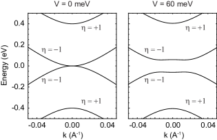
Figure 2: Electronic bands near the Dirac valley associated with $\tau=1$. On the left panel we show the case without bias, and on the right one the bands when a bias of $V=60$ meV is considered. For convenience we label the valence and conduction bands with an additional index $\eta$, which is equal to $-1$ for the bands closer to the middle of the gap and $1$ for the other two.

In this figure, we see that, for zero bias, one finds the usual bands of bilayer graphene, which host no gap since the lowest conduction band and the highest valence band touch at $k=0$. When the bias is increased to $V=60$ meV, the two aforementioned bands are deformed, taking the shape of a “Mexican hat”. This deformation of the valence and conduction bands leads to the opening of a gap, something crucial to exploit excitonic effects. If the next nearest neighbors hoppings had been considered only minor changes would appear in the band structure. Even though small, these modifications in the bands have an important effect on the optical selection rules (which we discuss ahead), since they introduce the trigonal warping effect, which reduces the symmetry of our calculation from $C_{\infty}$ to $C_{3}$.

From the diagonalization of Eq. (2), we also find the eigenvectors associated with each band. We label these vectors as $|c,\eta,\mathbf{k\rangle}$ and $|v,\eta,\mathbf{k}\rangle$, where the index $\eta$ is defined as in Fig. 2, i.e. the bands closer to the middle of the gap have $\eta=-1$, while the other two have $\eta=1$; they read:

$$|c,-1,\mathbf{k}\rangle =\left[a_{c,1}^{-}e^{i\tau\theta},a_{c,2}^{-},a_{c,3}^{-}e^{i\tau\theta},a_{c,4}^{-}e^{2i\tau\theta}\right]$$ (3)

$$|c,+1,\mathbf{k}\rangle =\left[a_{c,1}^{+},a_{c,2}^{+}e^{-i\tau\theta},a_{c,3}^{+},a_{c,4}^{+}e^{i\tau\theta}\right]$$ (4)

$$|v,-1,\mathbf{k}\rangle =\left[a_{v,1}^{-}e^{-i\tau\theta},a_{v,2}^{-}e^{-2i\tau\theta},a_{v,3}^{-}e^{-i\tau\theta},a_{v,4}^{-}\right]$$ (5)

$$|v,+1,\mathbf{k}\rangle =\left[a_{v,1}^{+},a_{v,2}^{+}e^{-i\tau\theta},a_{v,3}^{+},a_{v,4}^{+}e^{i\tau\theta}\right]$$ (6)

The specific definition of each entry is not of particular interest to the current analysis, however, the phase of each spinor was chosen carefully. As a consequence of the definition of $\theta$, as $k\rightarrow 0$ the complex exponential $e^{i\tau\theta}$ is discontinuous. To avoid this discontinuity in the eigenvectors, the phase of each one was chosen such that the complex exponentials appear multiplied by terms that vanish in the limit of small $k$. It is by now known that the phase choice of the Bloch factors plays a crucial role in determining the optical selection rules, and the criteria we established here is the one that directly leads to Hydrogen-like selection rules in the monolayer. Although other phase choices can be employed, they require the introduction of an additional angular quantum number associated with the pseudospin texture of the excitonic states [15, 21, 22]. Even though we do not shown the explicit form of the entries of each eigenvector, in light of the discussion regarding where the complex exponentials are place, it should be clear that $|a_{c,1}^{-}|,|a_{c,3}^{-}|,|a_{c,4}^{-}|\ll|a_{c,2}^{-}|$, $|a_{c,2}^{+}||a_{c,4}^{+}|\ll|a_{c,1}^{+}|,|a_{c,3}^{+}|$, $|a_{v,1}^{-}|,|a_{v,2}^{-}|,|a_{v,3}^{-}|\ll|a_{v,4}^{-}|$ and $|a_{v,2}^{+}||a_{v,4}^{+}|\ll|a_{v,1}^{+}|,|a_{v,3}^{+}|$. These relations between the amplitude of the different vector components are enough for us to gain intuition about the coupling strength of light with different excitonic states, which we introduce next.

III Bethe-Salpeter equation

Now that the single particle regime was studied, we move on to the excitonic part of the problem. To obtain the response of the system due to excitons we must first determine their energies and wave functions. These quantities can be obtained from the solution of the Bethe-Salpeter equation. This integral equation in momentum space may be written for a multi-band system as [23, 24]:

$$E\psi_{cv}(\mathbf{k}) =(E_{c,\mathbf{k}}-E_{v,\mathbf{k}})\psi_{cv}(\mathbf{k})$$

$$+\sum_{c^{\prime},v^{\prime}}\sum_{\mathbf{q}}V(\mathbf{k}-\mathbf{q})\langle c,\mathbf{k}|c^{\prime},\mathbf{q}\rangle\langle v^{\prime},\mathbf{q}|v,\mathbf{k}\rangle\psi_{cv}(\mathbf{q})$$ (7)

where, to simplify the notation, we omitted the index $\eta$ (which is now included in the indexes $c$ and $v$). We note that this equation takes the single particle energies $E_{c/v,\mathbf{k}}$ and eigenvectors $|c/v,\mathbf{k}\rangle$ as the input, and couples the different bands through an electrostatic potential $V(\mathbf{k}),$ thus capturing the many body nature intrinsic to excitons. By solving this equation, one finds the exciton energies, $E$, and the associated wave functions, $\psi_{cv}(\mathbf{k})$. In our approach we consider the electrostatic potential $V(\mathbf{k}-\mathbf{q})$ to be the Rytova-Keldysh potential [25, 26] (which is usually employed to describe excitonic effects in monolayers [5]). This potential can be obtained from the solution of the Poisson equation for a charge embedded in a thin film, by taking the limit of vanishing thickness. Although this potential presents a complex form in real space, its representation in momentum space is rather simple

$$V(\mathbf{k})=\frac{\hbar c\alpha}{\epsilon}\frac{1}{k(1+r_{0}k)},$$ (8)

where $\alpha\sim 1/137$, $\epsilon$ is the mean dielectric constant of the media above and below the bilayer and $r_{0}$ corresponds to an in plane screening length which is related to the 2D polarizability of the material; its value can be found from the single particle bands and Bloch factors. The numerical value of $r_{0}$ is of great importance to accurately describe the excitonic properties of a given system, since it directly affects the screening experienced by the carriers. Although the values of $r_{0}$ are well documented for TMDs, hBN and other 2D materials, the same is not true for biased bilayer graphene, where, in principle, $r_{0}$ varies with the bias $V$. In Ref. [27] the value of $r_{0}$ as a function of $V$ was determined, however, it was done using a 4 band tight binding model, which may not be sufficiently accurate. Ideally the value of $r_{0}$ should be determined from ab initio calculations taking into account several valence and conduction bands, because, as discussed in Ref. [28], depending on the material, a small number of bands of a minimal tight binding model may or may not be enough to accurately determine $r_{0}$. Since a detailed ab initio study of $r_{0}$ in BBLG is lacking in the literature, we will use the results of [27] as a reference. There one finds that, as expected, $r_{0}$ decreases with increasing band gap, or alternative, it decreases with increasing bias in a non-trivial way.

To solve the BSE we start by noting that Eq. (7) corresponds in fact to four equations, one for each possible pair $(v,c)$, forming an eigenvalue problem. To more easily solve the BSE, we assume that the excitons have a well defined angular quantum number $m$, such that $\psi_{cv}(\mathbf{k})=f_{cv}(k)e^{im\theta}$. Using this, and manipulating the phase choices of the spinors in Eq. (3), one can show that the BSE can be reduced to a 1D integral equation, which can then be efficiently solved with a single numerical quadrature (the details on how to achieve this are discussed in the Appendix).

After solving the BSE for a wide range of values for the bias (whilst using the results and parameters of the previous section, as well as the $r_{0}$ of Ref. [27] and taking $\epsilon=6.9$ [29], corresponding to the case of hBN encapsulated BLG), we observed that of the four possible sets of $\psi_{cv}(\mathbf{k})$, the contribution of the one with $\eta_{c}=\eta_{v}=-1$ was by far the dominant one, so much so, that the other wave functions appeared to vanish in comparison. This is a reasonable result to find, since intuition tells us that the bands with $\eta=-1$, i.e. the ones closer to the middle of the gap, should dominate the low energy response. Hence, to further optimize the calculation, one may restrict the BSE to a single pair of bands, thus greatly reducing the computational cost of the problem, without hindering the quality of the results.

IV Optical Absorption

In this section our goal is to determine the optical selection rules of the biased bilayer and to compute its optical absorption. To achieve both these goals we shall start by looking at the optical conductivity of the system. In the dipole approximation, and considering normal incidence, the optical conductivity follows as [24]

$$\sigma(\hbar\omega)\propto\sum_{n}\frac{\boldsymbol{\Omega}_{n}\boldsymbol{\Omega}_{n}^{*}}{\hbar\omega-E_{n}+i\frac{\Gamma_{n}}{2}}+\left(\omega\rightarrow-\omega\right)^{*},$$ (9)

where the sum over $n$ accounts for the different excitonic contributions with energy $E_{n}$, and the second term corresponds to the non-resonant part of the optical response. The quantity $\boldsymbol{\Omega}_{n}$ is defined as

$$\boldsymbol{\Omega}_{n}=\sum_{c,v}\sum_{\mathbf{k}}\psi_{cv}(\mathbf{k})\langle v,\mathbf{k}|\mathbf{r}|c,\mathbf{k}\rangle,$$ (10)

where $\langle v,\mathbf{k}|\mathbf{r}|c,\mathbf{k}\rangle$ is the interband matrix element of the dipole operator. Also, we introduced a phenomenological linewidth, $\Gamma_{n}$, which we assume to be $n-$dependent, to more easily compare our theoretical predictions with experimental data. As we have discussed before, we consider only the contribution of the bands with $\eta=-1$, since the $\psi_{cv}$ associated with the other ones are essentially zero. To evaluate the dipole matrix element we use the relation

$$\langle v,\mathbf{k}|\mathbf{r}|c,\mathbf{k}\rangle=\frac{\langle v,\mathbf{k}|\left[H,\mathbf{r}\right]|c,\mathbf{k}\rangle}{E_{v,\mathbf{k}}-E_{c,\mathbf{k}}}.$$ (11)

Although when solving the BSE we considered only the contribution of the nearest neighbor hoppings $\gamma_{0}$ and $\gamma_{1}$, to understand the role played by the other hoppings in the optical response, we shall take them into account when the commutator $\left[H,\mathbf{r}\right]$ is evaluated.

Let us now consider that our system is excited by a circularly polarized electric field. The relevant dipole matrix elements for such a situation are $\langle v,\mathbf{k}|x\pm iy|c,\mathbf{k}\rangle$, corresponding to positive and negative circular polarization. Using Eq. (11) to evaluate the matrix element, we find that the terms proportional to $\gamma_{0}$ give the contribution

$$\langle v,\mathbf{k}|x\pm iy|c,\mathbf{k}\rangle\big{|}_{\gamma_{0}} \propto\left(a_{c,2}^{-}a_{v,1}^{-}+a_{c,3}^{-}a_{v,4}^{-}\right)e^{i\tau\theta}\left(\tau\mp 1\right)$$

$$+\left(a_{c,1}^{-}a_{v,2}^{-}+a_{c,4}^{-}a_{v,3}^{-}\right)e^{3i\tau\theta}\left(\tau\pm 1\right).$$ (12)

It is then clear from Eq. (10), that such a result implies that only states with $m=-\tau$ and $m=-3\tau$, i.e. $p-$ and $f-$states, can be excited. From this result, one also sees that positive polarization excites states with $m=1$ in the valley with $\tau=-1$, and states with $m=-3$ in the opposite valley; an analogous results holds negative polarization. Regarding the coupling strength between the photons and the allowed exciton states, and recalling the comments made on the magnitude of eigenvector entries after Eq. (3), one can expect the resonances associated with the $p-$states to be far more intense than the ones associated with the $f-$states, which should present a vanishingly small oscillator strength. The contributions to the matrix element $\langle v,\mathbf{k}|x\pm iy|c,\mathbf{k}\rangle$ proportional to $\gamma_{3}$ and $\gamma_{4}$, lead to the same selection rules as the ones we have just discussed. Furthermore, since $\gamma_{1}\gg\gamma_{3},\gamma_{4}$, one finds that these hoppings can be safely ignored when studying the linear optical response of the bilayer. In stark contrast with this observation, the part of the dipole matrix element which is proportional to $\gamma_{5}$ introduces new selection rules. Explicitly:

$$\langle v,\mathbf{k}|x\pm iy|c,\mathbf{k}\rangle\big{|}_{\gamma_{5}} \propto a_{c,2}^{-}a_{v,4}^{-}\left(\tau\pm 1\right)$$

$$+a_{c,4}^{.-}a_{v,2}^{-}e^{4i\tau\theta}\left(\tau\mp 1\right),$$ (13)

where we see that by accounting for the contribution of $\gamma_{5}$, the excitation of $s-$ ($m=0$) and $g-$states $(m=\pm 4)$ becomes possible. Even though these contributions are proportional to $\gamma_{5}/\gamma_{0}\sim 0.1$, the large magnitude of $a_{c,2}^{-}a_{v,4}^{-}$ makes the $s-$states rather relevant for the optical response; the $g-$states, however, go totally unnoticed. A summary of the optical selection rules is depicted in Fig. 3 for $\tau=1$.

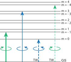
Figure 3: Schematic representation of the optical selection rules in the Dirac valley with $\tau=1$. Dashed lines indicate processes which are only possible with trigonal warping (TW). The thickness of the arrows illustrates the strength of the coupling with photons. The results for the $\tau=-1$ valley follow from these ones through the substitution $m\rightarrow-m$, and by switching the two circular polarizations. The ground state, i.e. the excitonic vacuum, is represented by GS

Since the two valleys are related through time reversal symmetry, the results for the $\tau=-1$ valley are identical given that one changes $m$ by $-m$, and switches the roles of the two circular polarizations. Moreover, since linear polarization can be viewed as the linear combination of the two circular polarization components, the analysis we performed is easily applied to the case of linearly polarized electric fields.

Having analyzed the optical selection rules of the biased bilayer, and making use of the solutions of the BSE, the optical conductivity is readily obtained. A quantity which is determined by the optical conductivity and is experimentally more relevant is the optical absorption. Here, we define the absorption as $\mathcal{A}=1-|r|^{2}-|t|^{2}$, where $r$ and $t$ are the reflection and transmission coefficients, respectively. These two coefficients are found from the longitudinal conductivity as [30]:

$$r (\hbar\omega)=\frac{\alpha\pi\sigma(\hbar\omega)/\sigma_{0}}{2\sqrt{\epsilon}+\alpha\pi\sigma_{L}/\sigma_{0}}$$ (14)

$$t(\hbar\omega) =\frac{2\sqrt{\epsilon}}{2\sqrt{\epsilon}+\alpha\pi\sigma(\hbar\omega)/\sigma_{0}},$$ (15)

with $\alpha\sim 1/137$, $\sigma(\hbar\omega)$ the optical conductivity and $\sigma_{0}=e^{2}/4\hbar$ the conductivity of a graphene monolayer.

Considering an in-plane linearly polarized electric field (for example along the $x$ direction), using once again $\epsilon=6.9$ (which describes a system encapsulated in hBN), and considering $\gamma_{5}=0.1\gamma_{1}$ [27], we find the absorption spectra depicted in Fig. 4 (a).

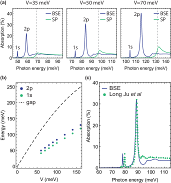
Figure 4: (a) Optical absorption of hBN encapsulated BBLG for three different values of the bias $V$. The blue line corresponds to the excitonic response obtained by using the solutions of the BSE; the green line gives the optical absorption in the single particle (SP) regime, obtained from Fermi’s golden rule. The dashed line indicates the location of the band gap. (b) Location of the 1s and 2p resonances as a function of the bias $V$. The dashed line gives the magnitude of the band gap. (c) Comparison between the experimental data of Ref. [16], and our theoretical prediction for a bias of $V=52$ meV.

Analyzing these results, we see that for each bias two resonances are well resolved, the smaller one at lower energies being due to the $1s$ exciton, and the larger one corresponding to the excitation of the $2p$ states. The linewidths of these resonances were chosen in order to match the experimentally measured values of Ref .[16], which read $\Gamma_{1s}=0.4$meV and $\Gamma_{2p}=1.3$meV. Although optically allowed, the $f-$ and $g-$states do not originate any noticeable resonance due to their small oscillator strength; the same is true for the more excited $s-$states. The more energetic $p-$states present a significant oscillator strength, however, since these are too close together, and too close to the band gap, they can hardly be resolved; instead, these states form the beginning of a plateau. This structure with an approximately constant magnitude is then extended beyond the band gap, due to the contribution of the interband excitations. Superimposed on the excitonic response, we also depict the interband conductivity obtained in the single particle (SP) picture using Fermi’s golden rule. This allows us to see that the excitonic effect is not only responsible for the resonances inside the gap, but also leads to a different response at higher energies, as a result of the shift in oscillator strength from the interband response to the excitonic resonances. The results of Fig. 4 (a) agree well with those of [15], which were obtained through more complex numerical approaches. Those results, however, do not account for the s-resonance which we include in our calculation.

Focusing now on the dependence of the absorption with the the bias, we observe that as the bias is increased the main features of the absorption remain qualitatively the same, but the optical response is shifted to higher energies. Further evidence of this behavior is given in panel (b) of the same figure where we depict the position of the $1s$ and $2s$ resonances as a function of the bias. This allows us to confirm that the resonances are in fact shifted to higher energies as the bias increases, while also becoming more separated from each other. The shift of the resonances to higher energies with increasing bias was to be expected, since, as we also depict, the band gap grows as the bias is turned up. However, we must note that the trend of the peak’s position differs slightly from that of the band gap. This is effect is due to dependence of $r_{0}$ with $V$, since as the bias increases, $r_{0}$ decreases, leading to more tightly bound excitons, appearing deeper into the gap. These two competing effects result in the almost linear dependence of the location of the resonances with $V$.

Finally, in panel (c) of Fig. 4, we compare our theoretical prediction with the experimental points of Long Ju and coworkers [16]. To facilitate the comparison between theory and experiment, we chose a bias of $V=52$ meV since it produced the best description of the experimental results; the remaining parameters retain the same values we considered so far (with $r_{0}$ taken from [27]). Comparing the theoretical prediction with the experimental data an excellent agreement is seen, in both the position and the magnitude of the two resonances. Besides this, we also see that the theoretical plateau at higher energies matches well with the experimental one. Although our plateau appears to be further away from the 2p resonance than in the experimental data, it seems possible to assign the structures that are experimentally captured on the high energy side of the largest peak to other excitonic state, which, due to their proximity, merge together, creating a single broader resonance.

At last, in Fig. 5, we depict a density plot of the $1s$ and $2p$ exciton wave functions for different bias.

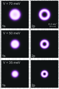
Figure 5: Density plot of the absolute value of the wavefunctions of the 1s and 2p states for three bias values $V=35$ meV, $V=50$ meV and $V=70$ meV. The same scaled is used in all panels.

As expected, for every case the $1s$ wave function is finite at $k=0$ while it vanishes for the $2p$ states. Moreover, as the bias increases the wave functions become more delocalized in momentum space. This increased delocalization in momentum space, translates to a higher localization in real space, in agreement with the aforementioned idea that the excitons become more tightly bound as the bias rises. This relation between real and momentum space also allows us to estimate the size of an exciton. Taking the case of $V=70$ meV as an example, we see that its $2p$ wave function presents a spread in momentum space of about $\Delta k=0.2$ nm^-1. Using $\Delta r=2\pi/\Delta k$, we estimate that the same exciton should be extended over approximately 40 nm in real space.

V Conclusion

In this paper we studied the excitonic response of biased bilayer graphene. To achieve this, we started by describing the single particle electronic properties of the system using a tight binding Hamiltonian. Afterwards, the single particle solutions were used as the input to the Bethe-Salpeter equation, whose solution defines the excitonic properties, i.e. their energies and wave functions. To solve the BSE we transformed the 2D integral equation into a 1D problem by carefully choosing the phase of the Bloch factors. This reduction in the dimension of the problem allows us to more efficiently solve the BSE, which now requires a single numerical quadrature.

To study the optical properties of the biased bilayer, we computed its conductivity, which allowed us to extract the optical selection rules and gain intuition on the strength of the photon-exciton coupling. We found that, in agreement with the literature, when trigonal warping is ignored, only $p-$states (with $m=\pm 1$) are bright; even though $f-$states are optically allowed they present a tiny oscillator strength. When trigonal warping is considered, and thus the symmetry of the calculation is reduced from $C_{\infty}$ to $C_{3}$, we find that $s-$states (with $m=0$) become optically allowed, and present a noticeable oscillator strength (at least for the 1s state).

Making use of the optical conductivity, we computed the absorption spectrum for the case where a biased bilayer graphene is encapsulated in hBN, which corresponds to the system where an experimental study was carried out by Long Ju and coworkers in [16]. Comparing our theoretical prediction with the experimental data, an excellent agreement was observed. Our model accurately described the position and magnitude of the 1s and 2p resonances, while also capturing the transition from excitonic resonances to the continuum of states, which originates the plateau that appears in the experimentally measured absorption. The dependence of the resonance’s location with the bias also agreed with the experimental data.

Note added: After the completion of this work we became aware of a similar unpublished work [31] on the same system we treated in this paper.

Appendix A On the solution of the Bethe-Salpeter equation

In this appendix we shall give a more in depth description on how to numerically solve the Bethe-Salpeter equation (BSE). This approach is an extension of the method presented in Ref. Ref. [32] to treat excitons in 2D semiconductors using the Coulomb potential. We take Eq. (7) of the main text as our starting point. Using the ansatz $\psi_{cv}(\mathbf{k})=f_{cv}(k)e^{im\theta}$, and taking the thermodynamic limit, we find:

$$\left(E_{k}^{c}-E_{k}^{v}\right)f_{cv}(k)-\frac{1}{4\pi^{2}}\sum_{c^{\prime}v^{\prime}}\int qdqd\theta_{q}V(\mathbf{k}-\mathbf{q})\langle u_{\mathbf{k}}^{c}|u_{\mathbf{q}}^{c^{\prime}}\rangle\langle u_{\mathbf{q}}^{v^{\prime}}|u_{\mathbf{k}}^{v}\rangle f_{c^{\prime}v^{\prime}}(q)e^{im\left(\theta_{q}-\theta_{k}\right)}=Ef_{cv}(k).$$ (16)

This equation corresponds to a two dimensional integral equation whose numerical solution is computationally demanding. To reduce the numerical weight of the calculation we wish to reduce the problem to that of a one dimensional integral equation. This can be achieved if the product of Bloch factors has the form

$$\langle u_{\mathbf{k}}^{c}|u_{\mathbf{q}}^{c^{\prime}}\rangle\langle u_{\mathbf{q}}^{v^{\prime}}|u_{\mathbf{k}}^{v}\rangle=\sum_{\lambda}\mathcal{A}_{\lambda}^{cc^{\prime}vv^{\prime}}(k,q)e^{i\lambda(\theta_{q}-\theta_{k})},$$ (17)

since this allows us to perform a variable change from to $\vartheta=\theta_{q}-\theta_{k}$, thus eliminating one of the momentum dependent integrals; here $\lambda$ is some integer, and $\mathcal{A}_{\lambda}^{cc^{\prime}vv^{\prime}}(k,q)$ are coefficients determined by the explicit computation of the spinor product. In principle this is always possible for the materials we are considering, given that the phases of the Bloch factors are appropriately chosen. Inserting this into the previous equation, and noting that $V(\mathbf{k}-\mathbf{q})\equiv V(k,q,\theta_{q}-\theta_{k})$, one finds

$$\left(E_{k}^{c}-E_{k}^{v}\right)f_{cv}(k)-\frac{1}{4\pi^{2}}\sum_{c^{\prime}v^{\prime}}\sum_{\lambda}\int qdqd\vartheta V(k,q,\vartheta)\mathcal{A}_{\lambda}^{cc^{\prime}vv^{\prime}}(k,q)f_{c^{\prime}v^{\prime}}(q)e^{i\left(m+\lambda\right)\vartheta}=Ef_{cv}(k),$$ (18)

where we explicitly introduced the variable change $d\theta_{q}\rightarrow d\vartheta$. Now, recalling the definition of Rytova-Keldysh potential $V(k,q,\vartheta)$, we introduce a new function, $\mathcal{I}_{\nu}(k,q)$ corresponding to the integral over $d\vartheta$:

$$\mathcal{I}_{\nu}(k,q)=\int_{0}^{2\pi}\frac{\cos\left(\nu\vartheta\right)}{\kappa(k,q,\vartheta)\left[1+r_{0}\kappa(k,q,\vartheta)\right]}d\vartheta$$ (19)

with $\kappa(k,q,\vartheta)=\sqrt{k^{2}+q^{2}-2kq\cos\vartheta}$. Notice how only $\cos(\nu\theta)$ enters the integral, since the analogous term in $\sin(\nu\vartheta)$ vanishes due to parity. From inspection, it should be clear that when $q=k$ the function $\mathcal{I}_{\nu}(k,q)$ is numerically ill-behaved, and as such must be treated carefully. For convenience we shall express $\mathcal{I}_{\nu}(k,q)$ in terms of partial fractions as

$$\mathcal{I}_{\nu}(k,q) =\int_{0}^{2\pi}\frac{\cos\left(\nu\vartheta\right)}{\kappa(k,q,\vartheta)}d\vartheta-r_{0}\int_{0}^{2\pi}\frac{\cos\left(\nu\vartheta\right)}{\left[1+r_{0}\kappa(k,q,\vartheta)\right]}d\vartheta$$ (20)

$$\equiv\mathcal{J}_{\nu}(k,q)-\mathcal{K}_{\nu}(k,q),$$ (21)

where from these two terms only the first one, $\mathcal{J}_{\nu}(k,q)$, is problematic when $k=q$. Before we explain how to avoid this numerical problem, let us first write the BSE in a more useful way. First, we write

$$\left(E_{k}^{c}-E_{k}^{v}\right)f_{cv}(k)-\sum_{c^{\prime}v^{\prime}}\sum_{\lambda}\int_{0}^{\infty}\left\{\mathcal{J}_{m+\lambda}(k,q)\mathcal{A}_{\lambda}^{cc^{\prime}vv^{\prime}}(k,q)f_{c^{\prime}v^{\prime}}(q)-\mathcal{K}_{m+\lambda}(k,q)\mathcal{A}_{\lambda}^{cc^{\prime}vv^{\prime}}(k,q)f_{c^{\prime}v^{\prime}}(q)\right\}qdq=Ef_{cv}(k).$$ (22)

Then, we define $\mathcal{B}_{m}^{cc^{\prime}vv^{\prime}}(k,q)=\sum_{\lambda}\mathcal{J}_{m+\lambda}(k,q)\mathcal{A}_{\lambda}^{cc^{\prime}vv^{\prime}}(k,q)$ and $\mathcal{C}_{m}^{cc^{\prime}vv^{\prime}}(k,q)=\sum_{\lambda}\mathcal{K}_{m+\lambda}(k,q)\mathcal{A}_{\lambda}^{cc^{\prime}vv^{\prime}}(k,q)$. Using these, one finds

$$\left(E_{k}^{c}-E_{k}^{v}\right)f_{cv}(k)-\sum_{c^{\prime}v^{\prime}}\int_{0}^{\infty}\mathcal{B}_{m}^{cc^{\prime}vv^{\prime}}(k,q)f_{c^{\prime}v^{\prime}}(q)qdq+\sum_{c^{\prime}v^{\prime}}\int_{0}^{\infty}\mathcal{C}_{m}^{cc^{\prime}vv^{\prime}}(k,q)f_{c^{\prime}v^{\prime}}(q)qdq=Ef_{cv}(k).$$ (23)

Let us now focus on the numerical problem associated with $\mathcal{B}_{m}^{cc^{\prime}vv^{\prime}}(k,q)$. To treat the divergence that appears when $k=q$, we introduce an auxiliary function $g_{m}(k,q)$ and introduce the modification

$$\int_{0}^{\infty}\mathcal{B}_{m}^{cc^{\prime}vv^{\prime}}(k,q)f_{c^{\prime}v^{\prime}}(q)qdq\rightarrow\int_{0}^{\infty}\left[\mathcal{B}_{m}^{cc^{\prime}vv^{\prime}}(k,q)f_{c^{\prime}v^{\prime}}(q)-g_{m}(k,q)f_{c^{\prime}v^{\prime}}(k)\right]qdq+f_{c^{\prime}v^{\prime}}(k)\int_{0}^{\infty}g_{m}(k,q)qdq,$$ (24)

with $g_{m}$ defined such that $\lim_{q\rightarrow k}\left[\mathcal{B}_{m}^{cc^{\prime}vv^{\prime}}(k,q)-g_{m}(k,q)\right]=0$. Following Ref. [32], we define $g_{m}$ as

$$g_{m}=\mathcal{B}_{m}^{cc^{\prime}vv^{\prime}}(k,q)\frac{2k^{2}}{k^{2}+q^{2}}$$ (25)

With the analytical part of the calculation taken care of, we shall now discuss how to numerically solve the equation we have arrived to. First, we introduce a variable change which transforms the improper integral over $[0,\infty)$, into one with finite integration limits, such as $[0,1]$. One possibility is to define $q=\tan[\pi x/2]$. Afterwards, we discretize the variables $k$ and $x$ (and consequently $q$):

$$\left(E_{k_{i}}^{c}-E_{k_{i}}^{v}\right)f_{cv}(k_{i})+\sum_{c^{\prime}v^{\prime}}\sum_{j=1}^{N}\mathcal{C}_{m}^{cc^{\prime}vv^{\prime}}(k_{i},q_{j})f_{c^{\prime}v^{\prime}}(q_{j})q_{j}\frac{dq}{dx_{j}}$$

$$-\sum_{c^{\prime}v^{\prime}}\sum_{j\neq i}\mathcal{B}_{m}^{cc^{\prime}vv^{\prime}}(k_{i},q_{j})f_{c^{\prime}v^{\prime}}(q_{j})q_{j}\frac{dq}{dx_{j}}w_{j}-f_{c^{\prime}v^{\prime}}(k_{i})\left\{\int_{0}^{\infty}g_{m}(k_{i},p)pdp-\sum_{j\neq i}g_{m}(k_{i},q_{j})q_{j}\frac{dq}{dx_{j}}\right\}=Ef_{cv}(k_{i})$$ (26)

where $N$ is the number of points and $w_{j}$ is the weight function of the chosen numerical quadrature; also, $q_{j}\equiv q(x_{j})$ and $dq/dx_{j}\equiv\left[dq/dx\right]_{x=x_{j}}$. Furthermore, we note that $\int_{0}^{\infty}g_{m}(k_{i},p)pdp$ is numerically well behaved as opposed to the original integral, $\int_{0}^{\infty}\mathcal{B}_{m}^{cc^{\prime}vv^{\prime}}(k_{i},p)pdp$. Depending on the problem, and on how localized the excitonic wave functions are in momentum space, it may be useful to split the original improper integral into regions, in order to allow for a thinner mesh in the relevant portion of $k$-space, and a coarser one in the region where the wave functions are already close to zero.

Regarding the choice of quadrature, we employ a Gauss-Legendre quadrature, which is defined as [33]

$$\int_{a}^{b}f(y)dy\approx\sum_{i=1}^{N}w_{i}f(y_{i})$$ (27)

where

$$y_{i}=\frac{a+b+(b-a)\xi_{i}}{2},$$ (28)

with $\xi_{i}$ the $i-$th zero of the Legendre polynomial $P_{N}(y)$, and

$$w_{i}=\frac{b-a}{(1-\xi_{i})^{2}\left[P^{\prime}_{N}(\xi_{i})\right]^{2}}$$ (29)

with $P^{\prime}_{N}(\xi_{i})\equiv\left[dP_{N}(y)/dy\right]_{y=\xi_{i}}$.

At last, the only thing left to do is to realize that this equation can be expressed as an eigenvalue problem of a $4N\times 4N$ matrix. This matrix can be thought of as a $4\times 4$ matrix of matrices, each one with dimensions $N\times N$. The 16 blocks come from the different combinations of the indexes $c$, $c^{\prime}$, $v$ and $v^{\prime}$, with each block corresponding to a $N\times N$ matrix stemming from the numerical discretization of the integral. Solving the eigenvalue problem one finds the exciton energies and wave functions.

References

- Novoselov et al. [2004] K. S. Novoselov, A. K. Geim, S. V. Morozov, D.-e. Jiang, Y. Zhang, S. V. Dubonos, I. V. Grigorieva, and A. A. Firsov, science 306, 666 (2004).
- Wang et al. [2018] G. Wang, A. Chernikov, M. M. Glazov, T. F. Heinz, X. Marie, T. Amand, and B. Urbaszek, Rev. Mod. Phys. 90, 021001 (2018).
- Carvalho et al. [2016] A. Carvalho, M. Wang, X. Zhu, A. S. Rodin, H. Su, and A. H. C. Neto, Nature Reviews Materials 1, 1 (2016).
- Caldwell et al. [2019] J. D. Caldwell, I. Aharonovich, G. Cassabois, J. H. Edgar, B. Gil, and D. Basov, Nature Reviews Materials 4, 552 (2019).
- Cudazzo et al. [2011] P. Cudazzo, I. V. Tokatly, and A. Rubio, Phys. Rev. B 84, 085406 (2011).
- Watanabe et al. [2004] K. Watanabe, T. Taniguchi, and H. Kanda, Nature materials 3, 404 (2004).
- Kubota et al. [2007] Y. Kubota, K. Watanabe, O. Tsuda, and T. Taniguchi, Science 317, 932 (2007).
- Schaibley et al. [2016] J. R. Schaibley, H. Yu, G. Clark, P. Rivera, J. S. Ross, K. L. Seyler, W. Yao, and X. Xu, Nature Reviews Materials 1, 1 (2016).
- Yu et al. [2017] H. Yu, G.-B. Liu, J. Tang, X. Xu, and W. Yao, Science advances 3, e1701696 (2017).
- Branny et al. [2017] A. Branny, S. Kumar, R. Proux, and B. D. Gerardot, Nature communications 8, 1 (2017).
- Epstein et al. [2020] I. Epstein, B. Terrés, A. J. Chaves, V.-V. Pusapati, D. A. Rhodes, B. Frank, V. Zimmermann, Y. Qin, K. Watanabe, T. Taniguchi, H. Giessen, S. Tongay, J. C. Hone, N. M. R. Peres, and F. H. L. Koppens, Nano letters 20, 3545 (2020).
- Castro et al. [2007] E. V. Castro, K. Novoselov, S. Morozov, N. Peres, J. L. Dos Santos, J. Nilsson, F. Guinea, A. Geim, and A. C. Neto, Physical review letters 99, 216802 (2007).
- Zhang et al. [2009] Y. Zhang, T.-T. Tang, C. Girit, Z. Hao, M. C. Martin, A. Zettl, M. F. Crommie, Y. R. Shen, and F. Wang, Nature 459, 820 (2009).
- Oostinga et al. [2008] J. B. Oostinga, H. B. Heersche, X. Liu, A. F. Morpurgo, and L. M. Vandersypen, Nature materials 7, 151 (2008).
- Park and Louie [2010] C.-H. Park and S. G. Louie, Nano letters 10, 426 (2010).
- Ju et al. [2017] L. Ju, L. Wang, T. Cao, T. Taniguchi, K. Watanabe, S. G. Louie, F. Rana, J. Park, J. Hone, F. Wang, et al., Science 358, 907 (2017).
- Fuchs et al. [2008] F. Fuchs, C. Rödl, A. Schleife, and F. Bechstedt, Phys. Rev. B 78, 085103 (2008).
- Komsa and Krasheninnikov [2013] H.-P. Komsa and A. V. Krasheninnikov, Phys. Rev. B 88, 085318 (2013).
- Galvani et al. [2016] T. Galvani, F. Paleari, H. P. C. Miranda, A. Molina-Sánchez, L. Wirtz, S. Latil, H. Amara, and F. m. c. Ducastelle, Phys. Rev. B 94, 125303 (2016).
- Di Sabatino et al. [2020] S. Di Sabatino, J. Berger, and P. Romaniello, Faraday Discussions 224, 467 (2020).
- Zhang et al. [2018] X. Zhang, W.-Y. Shan, and D. Xiao, Phys. Rev. Lett. 120, 077401 (2018).
- Cao et al. [2018] T. Cao, M. Wu, and S. G. Louie, Phys. Rev. Lett. 120, 087402 (2018).
- Taghizadeh and Pedersen [2019] A. Taghizadeh and T. G. Pedersen, Phys. Rev. B 99, 235433 (2019).
- Pedersen [2015] T. G. Pedersen, Phys. Rev. B 92, 235432 (2015).
- Rytova [1967] S. Rytova, Moscow University Physics Bulletin 22 (1967).
- Keldysh [1979] L. Keldysh, Sov. J. Exp. and Theor. Phys. Lett. 29, 658 (1979).
- Li and Appelbaum [2019] P. Li and I. Appelbaum, Phys. Rev. B 99, 035429 (2019).
- Tian et al. [2019] T. Tian, D. Scullion, D. Hughes, L. H. Li, C.-J. Shih, J. Coleman, M. Chhowalla, and E. J. Santos, Nano letters 20, 841 (2019).
- Laturia et al. [2018] A. Laturia, M. L. Van de Put, and W. G. Vandenberghe, npj 2D Materials and Applications 2, 1 (2018).
- Gonçalves and Peres [2016] P. A. D. Gonçalves and N. M. Peres, An introduction to graphene plasmonics (World Scientific, 2016).
- Sauer and Pedersen [2021] M. O. Sauer and T. G. Pedersen, arXiv preprint arXiv:2110.14428 (2021).
- Chao and Chuang [1991] C. Y.-P. Chao and S. L. Chuang, Phys. Rev. B 43, 6530 (1991).
- Kythe and Puri [2011] P. Kythe and P. Puri, Computational methods for linear integral equations (Springer Science & Business Media, 2011).