A Radon Transform on the Cylinder

Abstract

We define a parametric Radon transform $R$ that assigns to a Sobolev function on the cylinder $\mathbb{S}\times\mathbb{R}$ in $\mathbb{R}^{3}$ its mean values along sets $E_{\zeta}$ formed by the intersections of planes through the origin and the cylinder. We show that $R$ is a continuous operator, prove an inversion formula, provide a support theorem, as well as a characterization of its null space. We conclude by presenting a formula for the dual transform $R^{*}$. We show that $R$ and its dual $R^{*}$ are related to the right-sided and left-sided Chebyshev fractional integrals. Using this relationship, we characterize the null space of $R$ and $R^{*}$ and provide an inversion formula for $R^{*}$.

45Q05, 44A12, 42A16, 26A33

1 Introduction

The problem of reconstructing a function from its averages along submanifolds goes back to the $19^{th}$ century [14]. The pioneering works of Paul Funk [4] and Johann Radon [13] contain fundamental ideas that not only facilitated further developments in numerous fields of mathematics and physics, but lie at the heart of modern tomography, applications to homeland security and non-destructive testing in industry, to mention just a few applications [8].

A mapping that assigns to each sufficiently good function $f$ on a given manifold $X$ a collection of integrals of $f$ over submanifolds of $X$ is commonly called the Radon transform of $f$ [5, 7, 14]. However, the term Radon transform has a wide meaning and is used in diverse transforms of the kind [3, 9, 10, 12].

In this article we define a Radon-like transform $R$ that assigns to a Sobolev function on the cylinder $\mathbb{S}\times\mathbb{R}$ in $\mathbb{R}^{3}$ its mean values along sets $E_{\zeta}$ formed by the intersections of planes through the origin and the cylinder. Unlike the classical Radon transform, the parametric transform $R$ averages functions using the arclength measure $d\sigma$ on $\mathbb{S}$ and not $dS$, the arclength measure on $E_{\zeta}$. This simplification gives rise to a continuous and invertible transform on the cylinder with strong connections to fractional calculus. By using $d\sigma$ instead of the arclength measure $dS$ on $E_{\zeta}$ we also avoid issues that arise with the averaging of a function over sets of infinite arclength. To the best of our knowledge, this problem has not been considered in the existing literature.

This article is organized as follows. In Section 2, we introduce the parametric transform $R$. In Section 3, we present some auxiliary concepts and technical results needed for later sections. Section 4 and Section 5 are the core of this paper and contain our main results.

2 The Parametric Transform R

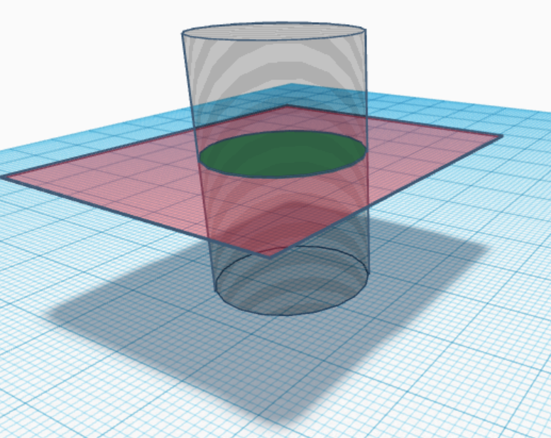
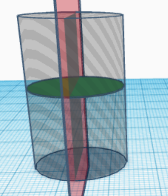
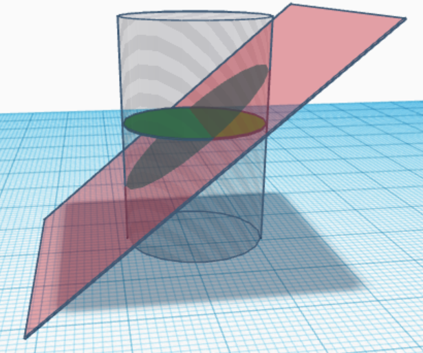
Figure 1: Geometry of sets $E_{\zeta(\theta,\rho)}$ for $\zeta(\theta,\rho)\in\mathbb{S}^{2}$ a pole, in the equator and elsewhere on $\mathbb{S}^{2}$.

We parametrize points on the cylinder $\mathbb{S}\times\mathbb{R}$ using local coordinates $s\in[0,2\pi)$ and $t\in\mathbb{R}$ by $(e^{is},t)$. We consider functions that are square integrable on the cylinder and whose weak partial derivatives $D^{\alpha}f$ exist and are square integrable for all multiindices $|\alpha|\leq 2$. We denote this function space $H^{2}(\mathbb{S}\times\mathbb{R})$ and note that it consists of functions that are continuous almost everywhere.

Consider the subset of $H^{2}(\mathbb{S}\times\mathbb{R})$

$$H^{2}_{pc}(\mathbb{S}\times\mathbb{R})=\left\{\left.f\in H^{2}(\mathbb{S}\times\mathbb{R})\right|\lim_{t\to\infty}f(e^{is},t)\stackrel{{\scriptstyle\mathclap{\mbox{\small a.e.}}}}{{\quad=\quad}}C(s)\text{ with }C\text{ integrable, }2\pi-\text{periodic}\right\}.$$

These functions behave nicely at infinity and allow their mean values along sets $E_{\zeta}$, formed by the intersection of planes through the origin and the cylinder, to converge.

The Radon-like operator $R$ assigns to functions in $H^{2}_{pc}(\mathbb{S}\times\mathbb{R})$ their mean values along sets $E_{\zeta}$ formed by the intersections of planes through the origin and the cylinder. The intersections of the cylinder $\mathbb{S}\times\mathbb{R}$ and planes through the origin define one of three different objects on $\mathbb{S}\times\mathbb{R}$, depending on the normal to the plane $\bm{\zeta}\in\mathbb{S}^{2}$ (Figure 1). The set of points resulting from the intersection of $\mathbb{S}\times\mathbb{R}$ and planes through the origin with normal $\bm{\zeta}$ given by a pole on $\mathbb{S}^{2}$ describes a circle. When $\bm{\zeta}$ lies on the equator of the sphere, the set describes two parallel lines on $\mathbb{S}\times\mathbb{R}$ perpendicular to the plane $z=0$. Finally, when the normal to the plane is neither a pole or in the equator of the sphere, the set $E_{\zeta}$ describes an ellipse.

We utilize the arclength measure $d\sigma$ on $\mathbb{S}$ to calculate the mean values of a function $f$ along the sets $E_{\zeta}$. Symbolically, we define the operator

(1) $$R:H^{2}_{pc}\rightarrow L^{2}(\mathbb{S}^{2})$$

(2) $$Rf(\zeta)\vcentcolon=\frac{1}{2\pi}\int_{E_{\zeta}}fd\sigma.$$

Granting the identification $\zeta=\zeta(\theta,\rho)=(\cos\theta\sin\rho,\sin\theta\sin\rho,\cos\rho)$ between $\mathbb{S}^{2}_{0}$, the $2-$dimensional sphere excluding the equator, and the set

$$(\theta,\rho)\in\Xi=[0,2\pi)\times[0,\pi]\setminus\{\pi/2\},$$

we may parametrize the sets $E_{\zeta(\theta,\rho)}$ by

$$E_{\zeta(\theta,\rho)} =\{x\in\mathbb{S}\times\mathbb{R}\enspace|\enspace\langle\,\zeta(\theta,\rho),x\,\rangle=0\,\}$$

$$=\{(e^{is},-\tan\rho\cos(\theta-s))\enspace|\enspace s\in[0,2\pi)\,\}.$$

This allows us to rewrite Eq. 2 as

(3) $$Rf(\theta,\rho)=\frac{1}{2\pi}\int_{0}^{2\pi}f(e^{is},-\tan\rho\cos(\theta-s))ds$$

for all $(\theta,\rho)\in\Xi$.

Proposition 2.1.

Let $f\in H^{2}_{pc}(\mathbb{S}\times\mathbb{R})$, then $Rf$ is well defined on $\mathbb{S}^{2}$.

Proof 2.2.

Let $f\in H^{2}_{pc}(\mathbb{S}\times\mathbb{R})$. By Theorem 3.2 there exits a bounded, continuous function that is equal to $f$ almost everywhere on $\mathbb{S}\times\mathbb{R}$. Without loss of generality, let $f$ denote this continuous representative. Since $R$ annihilates odd functions, assume that $f$ is even. Then,

$$Rf(\theta,\rho) =\frac{1}{2\pi}\int_{0}^{2\pi}f(e^{is},-\tan\rho\cos(\theta-s))\,ds$$

$$=\frac{1}{2\pi}\int_{\theta+\frac{\pi}{2}}^{\theta+\frac{5\pi}{2}}f(e^{is},-\tan\rho\cos(\theta-s))\,ds,$$

as the integrand is a $2\pi-$periodic function of $s$. Using the fact that $f$ is an even function on $\mathbb{S}\times\mathbb{R}$ and making a change of variables $r=s-\pi$ we obtain

$$Rf(\theta,\rho) =\frac{1}{\pi}\int_{\theta+\frac{\pi}{2}}^{\theta+\frac{3\pi}{2}}f(e^{is},-\tan\rho\cos(\theta-s))\,ds.$$

By hypothesis, there exists a $2\pi-$periodic function $C\in L^{1}([0,2\pi))$ such that

$$\lim_{t\to\infty}f(e^{is},t)\stackrel{{\scriptstyle\mathclap{\mbox{\small a.e.}}}}{{\quad=\quad}}C(s).$$

Since $f$ is bounded on $\mathbb{S}\times\mathbb{R}$, by the Lebesgue Dominated Convergence Theorem,

$$Rf(\theta,\pi/2) =\frac{1}{\pi}\lim_{\rho\to\pi/2}\,\int_{\theta+\frac{\pi}{2}}^{\theta+\frac{3\pi}{2}}f(e^{is},-\tan\rho\cos(\theta-s))\,ds$$

$$=\frac{1}{\pi}\int_{\theta+\frac{\pi}{2}}^{\theta+\frac{3\pi}{2}}\lim_{\rho\to\pi/2}f(e^{is},-\tan\rho\cos(\theta-s))\,ds$$

$$=\frac{1}{\pi}\int_{\theta+\frac{\pi}{2}}^{\theta+\frac{3\pi}{2}}C(s)\,ds$$

$$<\infty.$$

Therefore, we define the transform $R$ on the entire sphere $\mathbb{S}^{2}$, or equivalently in $\Xi\cup\{\pm\pi/2\}$, as

(4) $$Rf(\theta,\rho)\vcentcolon=\begin{cases}\frac{1}{2\pi}\int_{0}^{2\pi}f(e^{is},-\tan\rho\cos(\theta-s))ds&\quad\text{ if }(\theta,\rho)\in\Xi\\ &\\ \lim_{\varphi\to\pi/2}Rf(\theta,\varphi)&\quad\text{ if }(\theta,\rho)\in[0,2\pi)\times\{\pm\pi/2\}.\end{cases}$$

The following result is a corollary of Proposition 2.1 for a class of well behaved functions in $H^{2}_{pc}(\mathbb{S}\times\mathbb{R})$: functions that vanish at infinity.

Corollary 2.3.

Let $f\in H^{2}(\mathbb{S}\times\mathbb{R})$ be a function that vanishes at infinity. Then $Rf$ is well defined on $\mathbb{S}^{2}$ and $Rf(\theta,\pi/2)=0$ for all $\theta\in[0,2\pi)$.

3 Notation, Definitions & Technical Results

Let $\mathbb{S}\times\mathbb{R}$ be the $2-$dimensional cylinder in $\mathbb{R}^{3}$, $\mathbb{S}^{2}$ the $2-$dimensional sphere, $\mathbb{S}^{2}_{+}\subset\mathbb{S}^{2}$ the upper hemisphere of the sphere and $\mathbb{S}^{2}_{0}\subset\mathbb{S}^{2}$ the sphere excluding the equator.

Let $1\leq p<\infty$, then $L^{p}(\mathbb{S}\times\mathbb{R})$ denotes the usual Lebesgue function space of complex-valued functions on the cylinder. Let $k\in\{0,1,2,...\}$, we use $W^{k,p}(\mathbb{S}\times\mathbb{R})$ to denote the set of all Sobolev functions $f\in L^{p}(\mathbb{S}\times\mathbb{R})$ whose weak partial derivatives $D^{\alpha}f$ exist and belong to $L^{p}(\mathbb{S}\times\mathbb{R})$ for all $|\alpha|\leq k$. We use $H^{k}$ to distinguish the Hilbert spaces $H^{k}(\mathbb{S}\times\mathbb{R})=W^{k,2}(\mathbb{S}\times\mathbb{R})$ and $H^{k}_{pc}(\mathbb{S}\times\mathbb{R})\subset H^{k}(\mathbb{S}\times\mathbb{R})$ the subset of Sobolev functions on the cylinder that converge pointwise almost everywhere to some periodic function $C(s)\in L^{1}([0,2\pi))$ at infinity.

Theorem 3.1 and Theorem 3.2 are key tools for the results in this paper, as they guarantee the existence of a continuous and bounded function that is equal almost everywhere to $f\in H^{2}(\mathbb{S}\times\mathbb{R})$. We may use Theorem 3.2 for functions defined on the cylinder, since $\mathbb{S}\times\mathbb{R}$ is a complete Riemannian manifold of bounded curvature with injectivity radius $\delta=\pi$.

Theorem 3.1 ([1], Sobolev Embedding).

• Let $k$ and $\ell$ be two integers $(k>\ell\geq 0)$, $p$ and $q$ two real numbers $(1\leq q<p)$ satisfying $1/p=1/q-(k-\ell)/n$. Then, for $\mathbb{R}^{n}$, $W^{k,q}\subset W^{\ell,p}$ and the identity operator is continuous.

• If $(k-r)/n>1/q$, then $W^{k,q}\subset C^{r}_{B}$ and the identity operator is continuous. Here $r\geq 0$ is an integer and $C^{r}_{B}$ is the space of $C^{r}$ functions which are bounded as well as their derivatives of order less than or equal to $r$.

Theorem 3.2 ([1], Theorem 2.21).

Theorem 3.1 holds for $M_{n}$ a complete manifold with bounded curvature and injectivity radius $\delta>0$. Moreover, for any $\epsilon>0$, there exists a constant $A_{q}(\epsilon)$ such that every $\varphi\in W^{1,q}(M_{n})$ satisfies:

$$\|\varphi\|_{p}\leq[K(n,q)+\epsilon]\|\nabla\varphi\|_{q}+A_{q}(\epsilon)\|\varphi\|_{q}$$

with $1/p=1/q-1/n>0$, where $K(n,q)$ is the smallest constant having this property.

We use the following result to obtain the inversion formula in Section 4.

Lemma 3.3 ([2], Equation $16$).

Let $\ell\in\mathbb{N}\cup\{0\}$ and $r,z\in\mathbb{R}$ such that $0<z<r$, then

$$rz\int_{z}^{r}\frac{T_{\ell}\left(\frac{p}{z}\right)T_{\ell}\left(\frac{p}{r}\right)}{\sqrt{r^{2}-p^{2}}\sqrt{p^{2}-z^{2}}p}dp=\frac{\pi}{2}$$

where $T_{\ell}$ denotes the $\ell^{th}$ Chebyshev polynomial of the first kind

$$T_{\ell}(x)=\begin{cases}\cos(\ell\arccos x)&\qquad\text{if }|x|\leq 1,\\ \cosh(\ell\text{arcosh}x)&\qquad\text{if }x\geq 1,\\ (-1)^{\ell}\cosh(\ell\text{arcosh}(-x))&\qquad\text{if }x\leq-1.\end{cases}$$

Another set of major auxiliary results comes from fractional integrals, within the field of fractional calculus. In this paper we employ two fractional integral operators as defined by [15], the right-sided and left-sided Chebyshev fractional integrals. The formula for the right-sided Chebyshev fractional integral is given by

(5) $$\left(\Upsilon_{-}^{m}f\right)(t)=\frac{2}{\sqrt{\pi}}\int_{t}^{\infty}\frac{T_{m}\left(\frac{t}{r}\right)f(r)r}{\sqrt{r^{2}-t^{2}}}\,dr$$

and the left-sided Chebyshev fractional integral formula is given by

(6) $$\left(\Upsilon_{+}^{m}f\right)(r)=\frac{2}{\sqrt{\pi}}\int_{0}^{r}\frac{T_{m}\left(\frac{t}{r}\right)f(t)}{\sqrt{r^{2}-t^{2}}}\,dt.$$

We are particularly interested in knowing the conditions under which these operators converge.

Proposition 3.4 ([15], Proposition 2.46).

Let $a>0$, the integral $\left(\Upsilon_{-}^{m}f\right)(t)$ is finite for almost all $t>a$ under the following condition:

(7) $$\int_{a}^{\infty}|f(t)|t^{-\eta}\,dt<\infty\quad\text{ where }\quad\eta=\begin{cases}0&\quad\text{if }m\text{ is even,}\\ 1&\quad\text{if }m\text{ is odd.}\end{cases}$$

Proposition 3.5 ([15], Proposition 2.57).

Let $b>0$, the integral $\left(\Upsilon_{+}^{m}f\right)(r)$ is absolutely convergent for almost all $r<b$ under the following condition:

(8) $$\int_{0}^{b}t^{\eta}|f(t)|\,dt<\infty\quad\text{ where }\quad\eta=\begin{cases}0&\quad\text{if }m\text{ is even,}\\ 1&\quad\text{if }m\text{ is odd.}\end{cases}$$

Another property we are interested in is injectivity of operators Eq. 5 and Eq. 6. The following results show that the operators are not injective for for $|m|\geq 2$. In fact, for $|m|\geq 2$, [15] characterizes the null space for functions such that Eq. 9 and Eq. 10 hold.

Lemma 3.6 ([15], Lemma 2.49).

If $m=0,1$, then $\Upsilon_{-}^{m}$ is injective on $\mathbb{R^{+}}$ in the class of functions satisfying Eq. 7 for all $a>0$. If $m\geq 2$, then $\Upsilon_{-}^{m}$ is non-injective in this class of functions.

Lemma 3.7 ([15], Lemma 2.58).

If $m=0,1$, then $\Upsilon_{+}^{m}$ is injective on $\mathbb{R^{+}}$ in the class of functions satisfying Eq. 8 for all $b>0$. If $m\geq 2$, then $\Upsilon_{+}^{m}$ is non-injective in this class of functions.

Finally, if we let

$$\chi^{-}_{m}(t) =\begin{cases}1&\quad\text{if }m\text{ is even},\\ t^{-1}(1+|\log t|)&\quad\text{if }m\text{ is odd}\end{cases}$$

$$\chi^{+}_{m}(t) =\begin{cases}1&\quad\text{if }m\text{ is even},\\ t(1+|\log t|)&\quad\text{if }m\text{ is odd}\end{cases}$$

and given $a\geq 0$, we denote by $L_{\chi^{-}_{m}}^{1}(a,\infty)$ the set of all functions $f$ on $(a,\infty)$ such that

(9) $$\int_{a_{1}}^{\infty}|f(t)|\chi_{m}^{-}(t)\,dt<\infty\qquad\text{for all }a_{1}>a,$$

and for $0<b\leq\infty$, $L_{\chi^{+}_{m}}^{1}(0,b)$ the set of all functions $f$ on $(0,b)$ such that

(10) $$\int_{0}^{b_{1}}|f(t)|\chi_{m}^{+}(t)\,dt<\infty\qquad\text{for all }b_{1}<b,$$

then the following two lemmas characterize the null spaces of both operators for functions in $L^{1}_{\chi^{-}_{m}}(a,\infty)$ and $L^{1}_{\chi^{+}_{m}}(0,b)$.

Lemma 3.8 ([15], Lemma 2.62).

Let $m\in\mathbb{N}$ such that $m\geq 2$, $M=\left\lfloor\frac{m}{2}\right\rfloor$ and $a\geq 0$. If $f\in L_{\chi^{-}_{m}}^{1}(a,\infty)$ and $(\Upsilon_{-}^{m}f)(r)=0$ for almost all $r>a$, then for some coefficients $c_{k}$

$$f(t)=\sum_{k=0}^{M-1}c_{k}t^{2k-m}\qquad\text{a.e. on }(a,\infty).$$

Lemma 3.9 ([15], Lemma 2.61).

Let $m\in\mathbb{N}$ such that $m\geq 2$, $M=\left\lfloor\frac{m}{2}\right\rfloor$ and $b\geq 0$. If $f\in L_{\chi^{+}_{m}}^{1}(0,b)$ and $(\Upsilon_{+}^{m}f)(r)=0$ for almost all $0<r<b$, then for some coefficients $c_{j}$

$$f(t)=\sum_{j=1}^{M}c_{j}t^{m-2j}\qquad\text{a.e. on }(0,b).$$

The following two results are used to invert the dual transform of $R$ in Section 5.

Theorem 3.10 ([15], Theorem 2.44).

Let $f$ satisfy

$$\int_{a}^{\infty}|f(r)|dr<\infty\qquad\text{ for every }a>0.$$

Then

$$f(t)=(\textsc{D}^{\frac{1}{2}}_{-,2}I^{\frac{1}{2}}_{-,2}f)(t)$$

where

(11) $$\left(I^{\frac{1}{2}}_{-,2}f\right)(t) =\frac{2}{\sqrt{\pi}}\int_{t}^{\infty}\frac{f(r)r}{\sqrt{r^{2}-t^{2}}}dr$$

(12) $$\textsc{D}^{\frac{1}{2}}_{-,2}\varphi =-\frac{1}{2}\frac{d}{dt}tI^{\frac{1}{2}}_{-,2}t^{-2}\varphi,$$

and $t>0$.

Theorem 3.11 ([15], Corollary 2.52).

Let $m\in\mathbb{N}$ such that $n\geq 2$. Let $f$ be a function such that

$$\int_{a}^{\infty}|f(t)|t^{m-1}\,dt\qquad\text{ for all }a>0.$$

Then $f(t)$ can be uniquely reconstructed for almost all $t>0$ from the Chebyshev fractional integral $\Upsilon_{-}^{m}f=g$ by the formula

$$f(t)=-\frac{1}{2}\frac{d}{dt}\left(\overset{*}{\Upsilon}^{m}_{-}t^{-2}g\right)(t),$$

where

$$\left(\overset{*}{\Upsilon}^{m}_{-}g\right)(t)=\frac{2t}{\sqrt{\pi}}\int_{t}^{\infty}\frac{g(r)T_{m}\left(\frac{r}{t}\right)}{r\,\sqrt{r^{2}-t^{2}}}dr.$$

For the cases $m=0,1$, we first notice that

$$\Upsilon^{0}_{-}f =I^{\frac{1}{2}}_{-,2}f$$

$$\Upsilon^{1}_{-}f =tI^{\frac{1}{2}}_{-,2}t^{-1}f$$

where $I^{1/2}_{-,2}$ is defined by Eq. 11 and $t>0$. We may then find a unique solution to the equation $\Upsilon_{-}^{m}f=g$ for $m=0,1$ using Theorem 3.10.

4 Properties of R

Continuity

Theorem 4.1.

$R:H^{2}_{pc}(\mathbb{S}\times\mathbb{R})\rightarrow L^{2}(\mathbb{S}^{2})$ is a continuous transform.

Proof 4.2.

Let $f\in H^{2}_{pc}(\mathbb{S}\times\mathbb{R})$ and consider the norms

$$\|f\|_{2}^{2} =\int_{\mathbb{S}\times\mathbb{R}}\left|f(x)\right|^{2}dS(x)$$

$$=\int_{0}^{2\pi}\int_{-\infty}^{\infty}\left|f(e^{is},t)\right|^{2}dt\,ds$$

and

$$\|Rf\|_{2}^{2} =\int_{\mathbb{S}^{2}}\left|Rf(\zeta)\right|^{2}dS(\zeta)$$

$$=2\int_{0}^{2\pi}\int_{0}^{\frac{\pi}{2}}\left|Rf(\theta,\rho)\right|^{2}\sin\rho\,d\rho\,d\theta.$$

Now,

$$\int_{0}^{2\pi}\int_{0}^{\frac{\pi}{2}}\left|Rf(\theta,\rho)\right|^{2}\sin\rho\,d\rho\,d\theta \leq\int_{0}^{2\pi}\int_{0}^{\frac{\pi}{2}}\left(R|f|(\theta,\rho)\right)^{2}\sin\rho\,d\rho\,d\theta.$$

Using Jensen’s inequality, we obtain that

$$\left(R|f|(\theta,\rho)\right)^{2}\leq\frac{1}{2\pi}\int_{0}^{2\pi}\left|f(e^{is},-\tan\rho\cos(\theta-s))\right|^{2}ds.$$

Therefore,

$$\int_{0}^{2\pi}\int_{0}^{\frac{\pi}{2}}\left|Rf(\theta,\rho)\right|^{2}\sin\rho\,d\rho\,d\theta \leq\frac{1}{2\pi}\int_{0}^{2\pi}\int_{0}^{\frac{\pi}{2}}\int_{0}^{2\pi}\left|f(e^{is},-\tan\rho\cos(\theta-s))\right|^{2}\sin\rho\,ds\,d\rho\,d\theta.$$

Switching the order of integration, letting $\gamma=\theta-s+\pi$ with respect to $\theta$ and noticing that the integrand is $2\pi-$periodic with respect to the $\gamma$ variable, we obtain

$$\int_{0}^{2\pi}\int_{0}^{\frac{\pi}{2}}\left|Rf(\theta,\rho)\right|^{2}\sin\rho\,d\rho\,d\theta \leq\frac{1}{2\pi}\int_{0}^{2\pi}\int_{0}^{\frac{\pi}{2}}\int_{0}^{2\pi}\left|f(e^{is},\tan\rho\cos\gamma)\right|^{2}\sin\rho\,d\gamma\,d\rho\,ds$$

$$=\frac{1}{2\pi}\int_{0}^{2\pi}\int_{0}^{\frac{\pi}{2}}\int_{0}^{\pi}\left|f(e^{is},\tan\rho\cos\gamma)\right|^{2}\sin\rho\,d\gamma\,d\rho\,ds$$

$$\quad+\frac{1}{2\pi}\int_{0}^{2\pi}\int_{0}^{\frac{\pi}{2}}\int_{\pi}^{2\pi}\left|f(e^{is},\tan\rho\cos\gamma)\right|^{2}\sin\rho\,d\gamma\,d\rho\,ds$$

$$=\frac{1}{2\pi}\int_{0}^{2\pi}\int_{0}^{\frac{\pi}{2}}\int_{0}^{\pi}\left|f(e^{is},\tan\rho\cos\gamma)\right|^{2}\sin\rho\,d\gamma\,d\rho\,ds$$

$$\quad+\frac{1}{2\pi}\int_{0}^{2\pi}\int_{0}^{\frac{\pi}{2}}\int_{0}^{\pi}\left|f(e^{is},-\tan\rho\cos\theta)\right|^{2}\sin\rho\,d\theta\,d\rho\,ds.$$

Noting that $f$ is even, changing the order of integration and letting $u=s+\pi$ with respect to the $s$ variable, using the fact that the integrand is $2\pi-$periodic with respect to the new variable $u$ and switching the order of integration back again we obtain that

$$\int_{0}^{2\pi}\int_{0}^{\frac{\pi}{2}}\left|Rf(\theta,\rho)\right|^{2}\sin\rho\,d\rho\,d\theta$$

$$\qquad\leq\frac{1}{\pi}\int_{0}^{2\pi}\int_{0}^{\frac{\pi}{2}}\int_{0}^{\pi}\left|f(e^{is},\tan\rho\cos\gamma)\right|^{2}\sin\rho\,d\gamma\,d\rho\,ds$$

$$\qquad=\frac{1}{\pi}\int_{0}^{2\pi}\int_{0}^{\frac{\pi}{2}}\int_{0}^{\pi}\left|f(e^{is},\tan\rho\cos\gamma)\right|^{2}\sin\rho\,(\sin^{2}\gamma+\cos^{2}\gamma)\,d\gamma\,d\rho\,ds$$

$$\qquad=\frac{1}{\pi}\int_{0}^{2\pi}\int_{0}^{\frac{\pi}{2}}\int_{0}^{\pi}\left|f(e^{is},\tan\rho\cos\gamma)\right|^{2}\sin\rho\,\sin^{2}\gamma\,d\gamma\,d\rho\,ds$$

$$\qquad\quad+\frac{1}{\pi}\int_{0}^{2\pi}\int_{0}^{\frac{\pi}{2}}\int_{0}^{\pi}\left|f(e^{is},\tan\rho\cos\gamma)\right|^{2}\sin\rho\,\cos^{2}\gamma\,d\gamma\,d\rho\,ds$$

$$\qquad\leq\frac{1}{\pi}\int_{0}^{2\pi}\int_{0}^{\frac{\pi}{2}}\int_{0}^{\pi}\left|f(e^{is},\tan\rho\cos\gamma)\right|^{2}\sin\rho\,\sin\gamma\,d\gamma\,d\rho\,ds$$

$$\qquad\quad+\frac{1}{\pi}\int_{0}^{2\pi}\int_{0}^{\frac{\pi}{2}}\int_{0}^{\pi}\left|f(e^{is},\tan\rho\cos\gamma)\right|^{2}\sin\rho\,|\cos\gamma|\,d\gamma\,d\rho\,ds.$$

On the one hand,

$$\frac{1}{\pi}\int_{0}^{2\pi}\int_{0}^{\frac{\pi}{2}}\int_{0}^{\pi}\left|f(e^{is},\tan\rho\cos\gamma)\right|^{2}\sin\rho\,\sin\gamma\,d\gamma\,d\rho\,ds$$

$$\qquad=\frac{1}{\pi}\int_{0}^{2\pi}\int_{0}^{\frac{\pi}{2}}\int_{0}^{\pi}\left|f(e^{is},\tan\rho\cos\gamma)\right|^{2}\cos\rho\tan\rho\,\sin\gamma\,d\gamma\,d\rho\,ds$$

$$\qquad\leq\frac{1}{\pi}\int_{0}^{2\pi}\int_{0}^{\frac{\pi}{2}}\int_{0}^{\pi}\left|f(e^{is},\tan\rho\cos\gamma)\right|^{2}\tan\rho\,\sin\gamma\,d\gamma\,d\rho\,ds$$

$$\qquad=\frac{1}{\pi}\int_{0}^{2\pi}\int_{0}^{\frac{\pi}{2}}\int_{-\tan\rho}^{\tan\rho}\left|f(e^{is},t)\right|^{2}\,dt\,d\rho\,ds,$$

by letting $t=\tan\rho\cos\gamma$ with respect to the $\gamma$ variable. Therefore,

$$\frac{1}{\pi}\int_{0}^{2\pi}\int_{0}^{\frac{\pi}{2}}\int_{0}^{\pi}\left|f(e^{is},\tan\rho\cos\gamma)\right|^{2}\sin\rho\,\sin\gamma\,d\gamma\,d\rho\,ds$$

$$\qquad\leq\frac{1}{\pi}\int_{0}^{2\pi}\int_{0}^{\frac{\pi}{2}}\int_{-\infty}^{\infty}\left|f(e^{is},t)\right|^{2}\,dt\,d\rho\,ds$$

$$\qquad=\frac{1}{2}\int_{0}^{2\pi}\int_{-\infty}^{\infty}\left|f(e^{is},t)\right|^{2}\,dt\,ds.$$

Consequently,

$$\frac{1}{\pi}\int_{0}^{2\pi}\int_{0}^{\frac{\pi}{2}}\int_{0}^{\pi}\left|f(e^{is},\tan\rho\cos\gamma)\right|^{2}\sin\rho\,\sin\gamma\,d\gamma\,d\rho\,ds \leq\frac{1}{2}\int_{0}^{2\pi}\int_{-\infty}^{\infty}\left|f(e^{is},t)\right|^{2}\,dt\,ds.$$

On the other hand,

$$\frac{1}{\pi}\int_{0}^{2\pi}\int_{0}^{\frac{\pi}{2}}\int_{0}^{\pi}\left|f(e^{is},\tan\rho\cos\gamma)\right|^{2}\sin\rho\,|\cos\gamma|\,d\gamma\,d\rho\,ds$$

$$\qquad\leq\frac{1}{\pi}\int_{0}^{2\pi}\int_{0}^{\frac{\pi}{2}}\int_{0}^{\pi}\left|f(e^{is},\tan\rho\cos\gamma)\right|^{2}\,|\cos\gamma|\,d\gamma\,d\rho\,ds$$

$$\qquad=\frac{1}{\pi}\int_{0}^{2\pi}\int_{0}^{\frac{\pi}{2}}\int_{0}^{\frac{\pi}{2}}\left|f(e^{is},\tan\rho\cos\gamma)\right|^{2}\,\cos\gamma\,d\gamma\,d\rho\,ds$$

$$\qquad\quad-\frac{1}{\pi}\int_{0}^{2\pi}\int_{0}^{\frac{\pi}{2}}\int_{\frac{\pi}{2}}^{\pi}\left|f(e^{is},\tan\rho\cos\gamma)\right|^{2}\,\cos\gamma\,d\gamma\,d\rho\,ds$$

$$\qquad=\frac{1}{\pi}\int_{0}^{2\pi}\int_{0}^{\frac{\pi}{2}}\int_{0}^{\frac{\pi}{2}}\left|f(e^{is},\tan\rho\cos\gamma)\right|^{2}\,\cos\gamma\,d\rho\,d\gamma\,ds$$

$$\qquad\quad-\frac{1}{\pi}\int_{0}^{2\pi}\int_{\frac{\pi}{2}}^{\pi}\int_{0}^{\frac{\pi}{2}}\left|f(e^{is},\tan\rho\cos\gamma)\right|^{2}\,\cos\gamma\,d\rho\,d\gamma\,ds.$$

Let the change of variables $t=\tan\rho\cos\gamma$ with respect to $\rho$, then

$$\frac{1}{\pi}\int_{0}^{2\pi}\int_{0}^{\frac{\pi}{2}}\int_{0}^{\pi}\left|f(e^{is},\tan\rho\cos\gamma)\right|^{2}\sin\rho\,|\cos\gamma|\,d\gamma\,d\rho\,ds$$

$$\qquad\leq\frac{1}{\pi}\int_{0}^{2\pi}\int_{0}^{\frac{\pi}{2}}\int_{0}^{\infty}\left|f(e^{is},t)\right|^{2}\frac{\cos^{2}\gamma}{\cos^{2}\gamma+t^{2}}\,dt\,d\gamma\,ds$$

$$\qquad\quad+\frac{1}{\pi}\int_{0}^{2\pi}\int_{\frac{\pi}{2}}^{\pi}\int_{-\infty}^{0}\left|f(e^{is},t)\right|^{2}\frac{\cos^{2}\gamma}{\cos^{2}\gamma+t^{2}}\,dt\,d\gamma\,ds$$

$$\qquad\leq\frac{1}{\pi}\int_{0}^{2\pi}\int_{0}^{\frac{\pi}{2}}\int_{0}^{\infty}\left|f(e^{is},t)\right|^{2}\,dt\,d\gamma\,ds$$

$$\qquad\quad+\frac{1}{\pi}\int_{0}^{2\pi}\int_{\frac{\pi}{2}}^{\pi}\int_{-\infty}^{0}\left|f(e^{is},t)\right|^{2}\,dt\,d\gamma\,ds$$

$$\qquad=\frac{1}{2}\int_{0}^{2\pi}\int_{-\infty}^{\infty}\left|f(e^{is},t)\right|^{2}\,dt\,ds.$$

Consequently,

$$\frac{1}{\pi}\int_{0}^{2\pi}\int_{0}^{\frac{\pi}{2}}\int_{0}^{\pi}\left|f(e^{is},\tan\rho\cos\gamma)\right|^{2}\sin\rho\,|\cos\gamma|\,d\gamma\,d\rho\,ds \leq\frac{1}{2}\int_{0}^{2\pi}\int_{-\infty}^{\infty}\left|f(e^{is},t)\right|^{2}\,dt\,ds.$$

Therefore, putting both bounds together, we obtain

$$\int_{0}^{2\pi}\int_{0}^{\frac{\pi}{2}}\left|Rf(\theta,\rho)\right|^{2}\sin\rho\,d\rho\,d\theta \leq\int_{0}^{2\pi}\int_{-\infty}^{\infty}\left|f(e^{is},t)\right|^{2}\,dt\,ds,$$

or

$$\left\|Rf\right\|_{2}\leq\sqrt{2}\left\|f\right\|_{2}$$

and therefore, $R$ is continuous from $H^{2}_{pc}(\mathbb{S}\times\mathbb{R})$ to $L^{2}(\mathbb{S}^{2})$.

Null Space, Injectivity of R and an Inversion Formula

The transform $R$, just like the Funk transform, vanishes for all odd functions with respect to the equator. We will show that a necessary condition for a function space to have a non-trivial null space is that functions may not be bounded at infinity. To prove this we will make use of the following result.

Lemma 4.3.

Let $f\in H^{2}_{loc}(\mathbb{S}\times\mathbb{R})$ and $f(e^{is},t)=\sum_{n\in\mathbb{Z}}F_{n}(t)e^{ins}$ its Fourier series. Let $Rf(\theta,\rho)=\sum_{n\in\mathbb{Z}}G_{n}(\rho)e^{in\theta}$ be the Fourier series of $Rf$ on $\Xi$. Then

(13) $$G_{n}(\arctan x)=\frac{2(-1)^{|n|}}{\pi}\int_{0}^{x}\frac{F_{n}(v)T_{|n|}\left(\frac{v}{x}\right)}{\sqrt{x^{2}-v^{2}}}dv$$

where $x=\tan\rho$ and $T_{|n|}$ is the $|n|^{th}$ Chebyshev polynomial of the first kind.

Proof 4.4.

Let $f\in H^{2}_{loc}(\mathbb{S}\times\mathbb{R})$ and $(\theta,\rho)\in\Xi$. Since $f$ is in $H^{2}(E_{\zeta(\theta,\rho)})$, by Theorem 3.2 $f$ is equal almost everywhere to a continuous and bounded function on $E_{\zeta(\theta,\rho)}$. Without loss of generality, assume that $f$ is such representative. Since $R$ annihilates odd functions, assume that $f$ is an even function. Consequently, $Rf$ is an even function on $\Xi$ in the sense that $Rf(\theta,\rho)=Rf(\theta+\pi,\pi-\rho)$. Therefore, assume, without loss of generality, that $0\leq\rho<\pi/2$.

We parametrize the set $E_{\zeta(\theta,\rho)}$ as in Section 2 so that

$$Rf(\theta,\rho) =\frac{1}{2\pi}\int_{E_{\zeta(\theta,\rho)}}f(x)d\sigma(x)$$

$$=\frac{1}{2\pi}\int_{0}^{2\pi}f(e^{is},-\tan\rho\cos(\theta-s))ds.$$

Let $G_{n}(\rho)$ be the the $n^{th}$ Fourier coefficient of $Rf$. Then

$$G_{n}(\rho) =\frac{1}{2\pi}\int_{0}^{2\pi}Rf(\theta,\rho)e^{-in\theta}d\theta$$

$$=\frac{1}{4\pi^{2}}\int_{0}^{2\pi}\int_{0}^{2\pi}f(e^{is},-\tan\rho\cos(\theta-s))e^{-in\theta}ds\,d\theta.$$

Letting $u=s-\theta$, using the fact that the integrand is $2\pi-$periodic with respect to $u$, switching the order of integration, since $f$ is bounded on $E_{\zeta(\theta,\rho)}$, and letting $s=\theta+u$ we obtain

$$G_{n}(\rho) =\frac{1}{2\pi}\int_{0}^{2\pi}F_{n}(-\tan\rho\cos u)e^{-inu}du$$

$$=\frac{1}{2\pi}\left(\int_{0}^{\pi}F_{n}(-\tan\rho\cos u)e^{-inu}du+\int_{\pi}^{2\pi}F_{n}(-\tan\rho\cos u)e^{-inu}du\right)$$

$$=\frac{1}{2\pi}\left(\int_{0}^{\pi}F_{n}(-\tan\rho\cos u)e^{-inu}du+\int_{0}^{\pi}F_{n}(-\tan\rho\cos(v+\pi))e^{-in(v+\pi))}dv\right)$$

$$=\frac{1}{2\pi}\left(\int_{0}^{\pi}F_{n}(-\tan\rho\cos u)e^{-inu}du+\int_{0}^{\pi}(-1)^{|n|}F_{n}(\tan\rho\cos v)e^{-inv}dv\right).$$

By hypothesis $f$ is an even function on $\mathbb{S}\times\mathbb{R}$, therefore $F_{n}(t)=(-1)^{|n|}F_{n}(-t)$ and

$$G_{n}(\rho) =\frac{1}{\pi}\int_{0}^{\pi}F_{n}(-\tan\rho\cos u)e^{-inu}du.$$

The change of variables $v=-\tan\rho\cos u$ yields

$$G_{n}(\rho) =\frac{1}{\pi}\int_{0}^{\pi}F_{n}(-\tan\rho\cos u)e^{-inu}du$$

$$=\frac{1}{\pi}\int_{-\tan\rho}^{\tan\rho}F_{n}(v)e^{-in\arccos\left(\frac{-v}{\tan\rho}\right)}\frac{1}{\sqrt{\tan^{2}\rho-v^{2}}}dv$$

$$=\frac{1}{\pi}\int_{-\tan\rho}^{\tan\rho}F_{n}(v)e^{-in\left(\pi-\arccos\left(\frac{v}{\tan\rho}\right)\right)}\frac{1}{\sqrt{\tan^{2}\rho-v^{2}}}dv$$

$$=\frac{(-1)^{|n|}}{\pi}\int_{-\tan\rho}^{\tan\rho}F_{n}(v)e^{in\arccos\left(\frac{v}{\tan\rho}\right)}\frac{1}{\sqrt{\tan^{2}\rho-v^{2}}}dv.$$

Using Euler’s formula and the fact that $F_{n}(v)\sin(n\arccos(v/\tan\rho))/\sqrt{\tan^{2}\rho-v^{2}}$ is an odd function of $v$ yields

$$G_{n}(\rho) =\frac{(-1)^{|n|}}{\pi}\int_{-\tan\rho}^{\tan\rho}F_{n}(v)T_{|n|}\left(\frac{v}{\tan\rho}\right)\frac{1}{\sqrt{\tan^{2}\rho-v^{2}}}dv$$

$$=\frac{2(-1)^{|n|}}{\pi}\int_{0}^{\tan\rho}F_{n}(v)T_{|n|}\left(\frac{v}{\tan\rho}\right)\frac{1}{\sqrt{\tan^{2}\rho-v^{2}}}dv,$$

where $T_{|n|}$ is the $|n|^{th}$ Chebyshev polynomial.

Finally, letting $x=\tan\rho$

(14) $$G_{n}(\arctan x)=\frac{2(-1)^{|n|}}{\pi}\int_{0}^{x}\frac{F_{n}(v)T_{|n|}\left(\frac{v}{x}\right)}{\sqrt{x^{2}-v^{2}}}dv.$$

We obtain the following null space characterization when we define $R$ on the set of continuous functions on the cylinder.

Theorem 4.5.

Let $R:C(\mathbb{S}\times\mathbb{R})\rightarrow C(\mathbb{S}^{2}_{0})$. Then the null space of $R$ consists of all odd functions in $C(\mathbb{S}\times\mathbb{R})$ and those that are even and are such that their Fourier series $f(e^{is},t)=\sum_{n\in\mathbb{Z}}F_{n}(t)e^{ins}$ have polynomial coefficients

$$F_{n}(t)=0$$

for $|n|<2$, and

$$F_{n}(t)\stackrel{{\scriptstyle\mathclap{\mbox{\small a.e.}}}}{{\quad=\quad}}\sum_{m=1}^{\lfloor\frac{|n|}{2}\rfloor}a_{m}^{n}t^{|n|-2m}$$

for $|n|\geq 2$, where $a_{m}^{n}\in\mathbb{C}$.

Proof 4.6.

Let $(\theta,\rho)\in\Xi$, $x=\tan\rho$ and $f\in C(\mathbb{S}\times\mathbb{R})$. Consider the Fourier series $Rf(\theta,\rho)=\sum_{n\in\mathbb{Z}}G(\rho)e^{in\theta}$. Since $R$ annihilates odd functions, assume, without loss of generality, that $f$ is an even function. Hence, $Rf$ is an even function on $\Xi$ in the sense that $Rf(\theta,\rho)=Rf(\theta+\pi,\pi-\rho)$. Therefore, assume, without loss of generality, that $0\leq\rho<\pi/2$ so that $x>0$.

By Lemma 4.3

$$G_{n}(\arctan x)=\frac{2(-1)^{|n|}}{\pi}\int_{0}^{x}\frac{F_{n}(u)T_{|n|}\left(\frac{u}{x}\right)}{\sqrt{x^{2}-u^{2}}}du.$$

The right hand-side of the last equation may be expressed as a left-sided Chebyshev fractional integral as in Lemma 3.9 yielding

$$G_{n}(\arctan x)=\frac{(-1)^{|n|}}{\sqrt{\pi}}\left(\Upsilon_{+}^{|n|}F_{n}\right)(x).$$

Therefore,

$$Rf(\theta,\rho)=0 \iff\forall n\in\mathbb{Z}\quad G_{n}(\arctan x)=0.$$

By Lemma 3.7, $\Upsilon^{|n|}_{+}$ is injective for $|n|<2$. So for $|n|<2$, $G_{n}(\arctan x)=0$ if and only if $F_{n}\equiv 0$. For $|n|\geq 2$, by Lemma 3.9

$$F_{n}(t)\stackrel{{\scriptstyle\mathclap{\mbox{\small a.e.}}}}{{\quad=\quad}}\sum_{m=1}^{\lfloor\frac{|n|}{2}\rfloor}a_{m}^{n}t^{|n|-2m}$$

for some $a_{m}^{n}\in\mathbb{C}$.

Corollary 4.7.

The restriction of $R$ to the space of even functions in $H^{2}_{pc}$ is injective.

Proof 4.8.

All even functions $f\in H^{2}_{pc}(\mathbb{S}\times\mathbb{R})$ admit a bounded continuous representative by Theorem 3.2. Therefore, $f$ has bounded Fourier coefficients $F_{n}\in L^{1}_{\chi^{+}_{|n|}}(0,\infty)$ for all $n\in\mathbb{Z}$. Since the Fourier coefficients of functions in the nontrivial null space of $R$ are polynomials, therefore unbounded, this show that $R$ restricted to all even functions in $H^{2}_{pc}(\mathbb{S}\times\mathbb{R})$ has a trivial null space.

Theorem 4.9.

Let $f\in H^{2}_{loc}(\mathbb{S}\times\mathbb{R})$ and the Fourier series of $f$ on the cylinder be given by $f(e^{is},t)=\sum_{n\in\mathbb{Z}}F_{n}(t)e^{ins}$. Assume for some $\epsilon>0$, there are positive constants $C_{k}$, $k=0,1,...$ such that

(15) $$|F_{n}(t)|\leq\begin{cases}C_{0}&\quad\text{ if }n=0,\\ C_{n}|t|^{|n|-1}&\quad\text{ if }n\in\mathbb{Z}\setminus\{0\},\end{cases}$$

whenever $|t|<\epsilon$. Then $f$ can be recovered almost everywhere from the averages

$$Rf(\theta,\rho)=\frac{1}{2\pi}\int_{0}^{2\pi}f(e^{is},-\tan\rho\cos(\theta-s))ds$$

over all $\,(\theta,\rho)\in\Xi$. Moreover, for almost all $(e^{is},t)\in\mathbb{S}\times\mathbb{R}$ the function $f$ is given by

$$f(e^{is},t)=\sum_{n\in\mathbb{Z}}\left((-1)^{|n|}\frac{d}{dt}\int_{0}^{t}\frac{G_{n}(\arctan x)T_{|n|}\left(\frac{t}{x}\right)x}{\sqrt{t^{2}-x^{2}}}dx\right)e^{ins},$$

where $G_{n}$ is the $n^{th}$ Fourier coefficient of $Rf$ as in Lemma 4.3.

Proof 4.10.

Let $f\in H^{2}_{loc}(\mathbb{S}\times\mathbb{R})$. Since $R$ annihilates odd functions, assume that $f$ is an even function. Consequently, $Rf$ is an even function on $\Xi$ in the sense that $Rf(\theta,\rho)=Rf(\theta+\pi,\pi-\rho)$. Therefore, assume, without loss of generality, that $0\leq\rho<\pi/2$ so that $x=\tan\rho\geq 0$.

Let $Rf(\theta,\rho)=\sum_{n\in\mathbb{Z}}G_{n}(\rho)e^{in\theta}$. From Lemma 4.3

(16) $$G_{n}(\arctan x)=\frac{2(-1)^{|n|}}{\pi}\int_{0}^{x}\frac{F_{n}(u)T_{|n|}\left(\frac{u}{x}\right)}{\sqrt{x^{2}-u^{2}}}du,$$

where $x=\tan\rho$ and $T_{|n|}$ is the $|n|^{th}$ Chebyshev polynomial of the first kind.

Multiplying both sides of equation Eq. 16 by $T_{|n|}\left(\frac{t}{x}\right)x/\sqrt{t^{2}-x^{2}}$ and integrating with respect to $x$ from $0$ to some positive value $t$ yields

$$\int_{0}^{t}\frac{G_{n}(\arctan x)T_{|n|}\left(\frac{t}{x}\right)x}{\sqrt{t^{2}-x^{2}}}dx =\frac{2(-1)^{|n|}}{\pi}\int_{0}^{t}\int_{0}^{x}\frac{F_{n}(u)T_{|n|}\left(\frac{u}{x}\right)T_{|n|}\left(\frac{t}{x}\right)x}{\sqrt{t^{2}-x^{2}}\sqrt{x^{2}-u^{2}}}dudx.$$

Note that, by Eq. 15 the left-hand side is convergent and since $f\in H^{2}(\mathbb{S}\times[-t,t])$, by Theorem 3.2 $f$ is equal almost everywhere to a continuous and bounded function. Without loss of generality, we may assume that $f$ is such representative.

To change the order of integration, let us show that

$$\int_{0}^{t}\int_{0}^{x}\left|\frac{F_{n}(u)T_{|n|}\left(\frac{u}{x}\right)T_{|n|}\left(\frac{t}{x}\right)x}{\sqrt{t^{2}-x^{2}}\sqrt{x^{2}-u^{2}}}\right|du\,dx<\infty.$$

Without loss of generality, we may assume that $t<\epsilon$. Otherwise, we may split the integral into two parts: one where integration occurs over $x\in[\epsilon,t]$ and another one over $x\in(0,\epsilon)$. For the integral where $x$ is bounded away from zero, by continuity of $F_{n}$ and $T_{|n|}$, the numerator is bounded. The resulting integral is convergent and can be calculated using trigonometric substitution.

Since for all $n\in\mathbb{Z}$

$$\left|T_{|n|}(x)\right|\leq\begin{cases}1\qquad&\text{ for }|x|\leq 1,\\ |2x|^{|n|}\qquad&\text{ for }|x|>1,\end{cases}$$

we have that

$$\left|\frac{F_{n}(u)T_{|n|}\left(\frac{u}{x}\right)T_{|n|}\left(\frac{t}{x}\right)x}{\sqrt{t^{2}-x^{2}}\sqrt{x^{2}-u^{2}}}\right| \leq\left|\frac{F_{n}(u)\left(\frac{2t}{x}\right)^{|n|}x}{\sqrt{t^{2}-x^{2}}\sqrt{x^{2}-u^{2}}}\right|.$$

Noticing that $0\leq x\leq t$ we obtain the following bounds.

$$\left|\frac{F_{n}(u)T_{|n|}\left(\frac{u}{x}\right)T_{|n|}\left(\frac{t}{x}\right)x}{\sqrt{t^{2}-x^{2}}\sqrt{x^{2}-u^{2}}}\right| \leq\begin{cases}\left|\frac{F_{n}(u)(2t)}{\sqrt{t^{2}-x^{2}}\sqrt{x^{2}-u^{2}}}\right|&\quad\text{ for }|n|<2,\\ &\\ \left|\frac{F_{n}(u)(2t)^{|n|}}{x^{|n|-1}\sqrt{t^{2}-x^{2}}\sqrt{x^{2}-u^{2}}}\right|&\quad\text{ for }|n|\geq 2.\end{cases}$$

By hypothesis, there exists a value $\epsilon>0$ for which

$$|F_{n}(t)|\leq\begin{cases}C_{0}&\quad\text{ if }n=0,\\ C_{n}|t|^{|n|-1}&\quad\text{ if }n\in\mathbb{Z}\setminus\{0\},\end{cases}$$

for $t<\epsilon$. Hence, for all $|n|<2$

$$\int_{0}^{t}\int_{0}^{x}\left|\frac{F_{n}(u)x}{\sqrt{t^{2}-x^{2}}\sqrt{x^{2}-u^{2}}}\right|du\,dx \leq(2t)\int_{0}^{t}\frac{1}{\sqrt{t^{2}-x^{2}}}\int_{0}^{x}\frac{\left|F_{n}(u)\right|}{\sqrt{x^{2}-u^{2}}}\,du\,dx$$

$$\leq(2t)C_{n}\int_{0}^{t}\frac{1}{\sqrt{t^{2}-x^{2}}}\int_{0}^{x}\frac{1}{\sqrt{x^{2}-u^{2}}}\,du\,dx$$

$$\leq\frac{t\pi^{2}C_{n}}{2}$$

$$<\infty.$$

Similarly, for $|n|\geq 2$

$$\int_{0}^{t}\int_{0}^{x}\left|\frac{F_{n}(u)T_{|n|}\left(\frac{u}{x}\right)T_{|n|}\left(\frac{t}{x}\right)x}{\sqrt{t^{2}-x^{2}}\sqrt{x^{2}-u^{2}}}\right|du\,dx \leq(2t)^{|n|}\int_{0}^{t}\frac{1}{x^{|n|-1}\sqrt{t^{2}-x^{2}}}\int_{0}^{x}\frac{\left|F_{n}(u)\right|}{\sqrt{x^{2}-u^{2}}}\,du\,dx$$

$$=(2t)^{|n|}C_{n}\int_{0}^{t}\frac{1}{x^{|n|-1}\sqrt{t^{2}-x^{2}}}\int_{0}^{x}\frac{u^{|n|-1}}{\sqrt{x^{2}-u^{2}}}du\,dx.$$

The changes of variables $v=\sqrt{x^{2}-u^{2}}$ yields

$$\int_{0}^{t}\int_{0}^{x}\left|\frac{F_{n}(u)T_{|n|}\left(\frac{u}{x}\right)T_{|n|}\left(\frac{t}{x}\right)x}{\sqrt{t^{2}-x^{2}}\sqrt{x^{2}-u^{2}}}\right|du\,dx \leq(2t)^{|n|}C_{n}\int_{0}^{t}\frac{1}{x^{|n|-1}\sqrt{t^{2}-x^{2}}}\int_{0}^{x}(x^{2}-v^{2})^{\frac{|n|-2}{2}}dv\,dx$$

$$\leq(2t)^{|n|}C_{n}\int_{0}^{t}\frac{1}{x^{|n|-1}\sqrt{t^{2}-x^{2}}}\int_{0}^{x}x^{|n|-2}dv\,dx$$

$$=(2t)^{|n|}C_{n}\int_{0}^{t}\frac{1}{\sqrt{t^{2}-x^{2}}}dx$$

$$=\frac{(2t)^{|n|}\pi C_{n}}{2}$$

$$<\infty.$$

Therefore, we may interchange the order of integration to obtain

$$\int_{0}^{t}\frac{G_{n}(\arctan x)T_{|n|}\left(\frac{t}{x}\right)x}{\sqrt{t^{2}-x^{2}}}dx =\frac{2(-1)^{|n|}}{\pi}\int_{0}^{t}F_{n}(u)\left(\int_{u}^{t}\frac{T_{|n|}\left(\frac{u}{x}\right)T_{|n|}\left(\frac{t}{x}\right)x}{\sqrt{t^{2}-x^{2}}\sqrt{x^{2}-u^{2}}}dx\right)du.$$

Make the change of variables $v=u^{2}/x$ to obtain

$$\int_{0}^{t}\frac{G_{n}(\arctan x)T_{|n|}\left(\frac{t}{x}\right)x}{\sqrt{t^{2}-x^{2}}}dx =\frac{2(-1)^{|n|}}{\pi}\int_{0}^{t}F_{n}(u)\left(u\frac{u^{2}}{t}\int_{\frac{u^{2}}{t}}^{u}\frac{T_{|n|}\left(\frac{v}{u}\right)T_{|n|}\left(\frac{v}{(u^{2}/t)}\right)}{\sqrt{u^{2}-v^{2}}\sqrt{v^{2}-\left(\frac{u^{2}}{t}\right)^{2}}v}dv\right)du.$$

By Lemma 3.3, the expression in parentheses is equal to $\pi/2$. Therefore,

$$(-1)^{|n|}\int_{0}^{t}\frac{G_{n}(\arctan x)T_{|n|}\left(\frac{t}{x}\right)x}{\sqrt{t^{2}-x^{2}}}dx=\int_{0}^{t}F_{n}(u)du.$$

Using the Fundamental Theorem of Calculus, we obtain the following expression for the $n^{th}$ Fourier coefficient of $f$:

(17) $$F_{n}(t)=(-1)^{|n|}\frac{d}{dt}\int_{0}^{t}\frac{G_{n}(\arctan x)T_{|n|}\left(\frac{t}{x}\right)x}{\sqrt{t^{2}-x^{2}}}dx.$$

Substituting in the Fourier series of $f$ yields

(18) $$f(e^{is},t)=\sum_{n\in\mathbb{Z}}\left((-1)^{|n|}\frac{d}{dt}\int_{0}^{t}\frac{G_{n}(\arctan x)T_{|n|}\left(\frac{t}{x}\right)x}{\sqrt{t^{2}-x^{2}}}dx\right)e^{ins}.$$

Support Theorem

Notice that Theorem 4.9 depends only on the local behavior of $f$ near the equator and is independent of its behavior at infinity. Similarly, the following support theorem depends only on $Rf$ vanishing for $\rho\in[0,\arctan t]$ to determine that $f(e^{is},t)=0$ for all $s\in[0,2\pi)$.

Theorem 4.11 (Support Theorem).

Let $f\in H^{2}_{loc}(\mathbb{S}\times\mathbb{R})$ and the Fourier series of $f$ on the cylinder be given by $f(e^{is},t)=\sum_{n\in\mathbb{Z}}F_{n}(t)e^{ins}$. Assume for some $\epsilon>0$, there are positive constants $C_{k}$, $k=0,1,...$ such that

$$|F_{n}(t)|\leq\begin{cases}C_{0}&\quad\text{ if }n=0,\\ C_{n}|t|^{|n|-1}&\quad\text{ if }n\in\mathbb{Z}\setminus\{0\},\end{cases}$$

whenever $|t|<\epsilon$. Then for a fix $\theta\in[0,2\pi)$ and $t\in[0,\infty)$ and all $s\in[0,2\pi)$, the values of $f(e^{is},t)$ are completely determined by all values $Rf(\theta,\rho)$ for $\rho\in[0,\arctan t]$. In particular, if $Rf(\theta,\rho)\equiv 0$ for all $\rho\in[0,\arctan t]$, then $f(e^{is},t)=0$ for all $s\in[0,2\pi)$.

Proof 4.12.

By Theorem 4.9

$$f(e^{is},t)=\sum_{n\in\mathbb{Z}}\left((-1)^{|n|}\frac{d}{dt}\int_{0}^{t}\frac{G_{n}(\arctan x)T_{|n|}\left(\frac{t}{x}\right)x}{\sqrt{t^{2}-x^{2}}}dx\right)e^{ins}.$$

Now

$$Rf(\theta,\rho)\equiv 0\text{ for all }\rho\in[0,\arctan t] \iff Rf(\theta,\rho)=\sum_{n\in\mathbb{Z}}G_{n}(\rho)e^{in\theta}=0\text{ for all }\rho\in[0,\arctan t]$$

$$\iff G_{n}(\rho)\equiv 0\text{ for all }n\in\mathbb{Z}\text{ and }\rho\in[0,\arctan t].$$

Thus,

$$\int_{0}^{t}\frac{G_{n}(\arctan x)T_{|n|}\left(\frac{t}{x}\right)x}{\sqrt{t^{2}-x^{2}}}dx=0$$

and $f(e^{is},t)=0$ for all $s\in[0,2\pi)$.

5 The Dual Transform

In this section we study the dual transform $R^{*}$. The dual will be defined as the formal adjoint of $R$ in the sense that, for $g\in C(\mathbb{S}^{2})$ and $f\in H^{2}_{pc}(\mathbb{S}\times\mathbb{R})$, $R^{*}g$ satisfies the duality relation

$$\int_{0}^{2\pi}\int_{0}^{\pi}Rf(\theta,\rho)\overline{g(\theta,\rho)}|\sin\theta|\,d\rho\,d\theta=\int_{0}^{2\pi}\int_{-\infty}^{\infty}f(e^{is},t)\overline{R^{*}g(e^{is},t)}\,dt\,ds.$$

The following theorem gives us an explicit formula for $R^{*}$.

Theorem 5.1.

Let $g\in C(\mathbb{S}^{2})$ be an even function and $f\in H^{2}_{pc}(\mathbb{S}\times\mathbb{R})$. Then the formal adjoint of $R$ is given by the formula

$$R^{*}g(e^{is},t) =\frac{1}{\pi}\sum_{\sigma=\pm 1}\,\int^{\infty}_{0}g\left(s+\sigma\arccos\left(\frac{-t}{\sqrt{v^{2}+t^{2}}}\right),\arctan\sqrt{v^{2}+t^{2}}\right)\,\frac{dv}{(1+v^{2}+t^{2})^{\frac{3}{2}}}$$

for $(e^{is},t)\in\mathbb{S}\times\mathbb{R}$.

Proof 5.2.

Let $f\in H^{2}_{pc}(\mathbb{S}\times\mathbb{R})$. Since $R$ annihilates odd functions and by Theorem 3.2, without loss of generality, assume that $f$ is a continuous, bounded and even function on $\mathbb{S}\times\mathbb{R}$. Let $g\in C(\mathbb{S}^{2})$ be even in the sense that

$$g(\theta,\rho)=g(\theta+\pi,\pi-\rho)$$

for all $\theta\in[0,2\pi)$ and $\rho\in[0,\pi]$. Then,

$$\langle Rf,g\rangle_{\mathbb{S}^{2}} =\int_{0}^{2\pi}\int_{0}^{\pi}Rf(\theta,\rho)\overline{g(\theta,\rho)}\,\sin\rho\,d\rho\,d\theta$$

$$=\frac{1}{2\pi}\int_{0}^{2\pi}\int_{0}^{\pi}\int_{0}^{2\pi}f\left(e^{is},-\tan\rho\cos(\theta-s)\right)\overline{g(\theta,\rho)}\,\sin\rho\,ds\,d\rho\,d\theta$$

$$=\frac{1}{2\pi}\int_{0}^{2\pi}\int_{0}^{\pi}\int_{-s}^{2\pi-s}f\left(e^{is},-\tan\rho\cos u\right)\overline{g(u+s,\rho)}\,\sin\rho\,du\,d\rho\,ds,$$

by switching the order of integration and letting $u=\theta-s$ with respect to the $\theta$ variable.

Since both $\cos u$ and $g(u+s,\rho)$ are $2\pi-$periodic functions of $u$, we can change the inner most limits of integration to obtain

$$\langle Rf,g\rangle_{\mathbb{S}^{2}} =\frac{1}{2\pi}\int_{0}^{2\pi}\int_{0}^{\pi}\int_{0}^{2\pi}f\left(e^{is},-\tan\rho\cos u\right)\overline{g(u+s,\rho)}\,\sin\rho\,du\,d\rho\,ds$$

$$=\frac{1}{2\pi}\int_{0}^{2\pi}\int_{0}^{\pi}\int_{0}^{\pi}f\left(e^{is},-\tan\rho\cos u\right)\overline{g(u+s,\rho)}\,\sin\rho\,du\,d\rho\,ds$$

$$\quad+\frac{1}{2\pi}\int_{0}^{2\pi}\int_{0}^{\pi}\int_{\pi}^{2\pi}f\left(e^{is},-\tan\rho\cos u\right)\overline{g(u+s,\rho)}\,\sin\rho\,du\,d\rho\,ds.$$

Since $f$ is even, letting $v=u-\pi$ in the last integral yields

$$\langle Rf,g\rangle_{\mathbb{S}^{2}} =\frac{1}{2\pi}\int_{0}^{2\pi}\int_{0}^{\pi}\int_{0}^{\pi}f\left(e^{is},-\tan\rho\cos u\right)\overline{g(u+s,\rho)}\,\sin\rho\,du\,d\rho\,ds$$

$$\quad+\frac{1}{2\pi}\int_{0}^{2\pi}\int_{0}^{\pi}\int_{0}^{\pi}f\left(e^{i(s+\pi)},-\tan\rho\cos v\right)\overline{g(v+(s+\pi),\rho)}\,\sin\rho\,dv\,d\rho\,ds.$$

By switching the order of integration, letting $\omega=s+\pi$ with respect to the $s$ variable, using the fact that the integrand is $2\pi-$periodic with respect to the new variable $\omega$, switching back the order of integration and renaming the $\omega$ variable $s$ we obtain

$$\langle Rf,g\rangle_{\mathbb{S}^{2}} =\frac{1}{\pi}\int_{0}^{2\pi}\int_{0}^{\pi}\int_{0}^{\pi}f\left(e^{is},-\tan\rho\cos u\right)\overline{g(s+u,\rho)}\,\sin\rho\,du\,d\rho\,ds$$

Letting $t=-\tan\rho\cos u$ with respect to the $u$ variable yields

$$\langle Rf,g\rangle_{\mathbb{S}^{2}} =\frac{1}{\pi}\int_{0}^{2\pi}\int_{0}^{\pi}\int_{-\tan\rho}^{\tan\rho}f\left(e^{is},t\right)\overline{g\left(s+\arccos\left(\frac{-t}{\tan\rho}\right),\rho\right)}\,\frac{\sin\rho}{\sqrt{\tan^{2}\rho-t^{2}}}\,dt\,d\rho\,ds$$

$$=\frac{1}{\pi}\int_{0}^{2\pi}\int_{0}^{\pi/2}\int_{-\tan\rho}^{\tan\rho}f\left(e^{is},t\right)\overline{g\left(s+\arccos\left(\frac{-t}{\tan\rho}\right),\rho\right)}\,\frac{\sin\rho}{\sqrt{\tan^{2}\rho-t^{2}}}\,dt\,d\rho\,ds$$

$$\quad-\frac{1}{\pi}\int_{0}^{2\pi}\int_{\pi/2}^{\pi}\int_{\tan\rho}^{-\tan\rho}f\left(e^{is},t\right)\overline{g\left(s+\arccos\left(\frac{-t}{\tan\rho}\right),\rho\right)}\,\frac{\sin\rho}{\sqrt{\tan^{2}\rho-t^{2}}}\,dt\,d\rho\,ds$$

Splitting the innermost integrals, switching the order of integration and noting that for $t<0$ we have that $-\arctan t=\arctan|t|$ and $\arctan t=-\arctan|t|$ yields

$$\langle Rf,g\rangle_{\mathbb{S}^{2}} =\frac{1}{\pi}\int_{0}^{2\pi}\int_{-\infty}^{0}\int_{\arctan|t|}^{\pi/2}f\left(e^{is},t\right)\overline{g\left(s+\arccos\left(\frac{-t}{\tan\rho}\right),\rho\right)}\,\sin\rho\,\frac{\,d\rho\,dt\,ds}{\sqrt{\tan^{2}\rho-t^{2}}}$$

$$\quad+\frac{1}{\pi}\int_{0}^{2\pi}\int_{0}^{\infty}\int_{\arctan|t|}^{\pi/2}f\left(e^{is},t\right)\overline{g\left(s+\arccos\left(\frac{-t}{\tan\rho}\right),\rho\right)}\,\sin\rho\,\frac{\,d\rho\,dt\,ds}{\sqrt{\tan^{2}\rho-t^{2}}}$$

$$\quad-\frac{1}{\pi}\int_{0}^{2\pi}\int_{-\infty}^{0}\int_{\pi/2}^{\pi-\arctan|t|}f\left(e^{is},t\right)\overline{g\left(s+\arccos\left(\frac{-t}{\tan\rho}\right),\rho\right)}\,\sin\rho\,\frac{\,d\rho\,dt\,ds}{\sqrt{\tan^{2}\rho-t^{2}}}$$

$$\quad-\frac{1}{\pi}\int_{0}^{2\pi}\int_{0}^{\infty}\int_{\pi/2}^{\pi-\arctan|t|}f\left(e^{is},t\right)\overline{g\left(s+\arccos\left(\frac{-t}{\tan\rho}\right),\rho\right)}\,\sin\rho\,\frac{\,d\rho\,dt\,ds}{\sqrt{\tan^{2}\rho-t^{2}}}$$

Therefore,

$$\langle Rf,g\rangle_{\mathbb{S}^{2}} =\frac{1}{\pi}\int_{0}^{2\pi}\int_{-\infty}^{\infty}\int_{\arctan|t|}^{\pi/2}f\left(e^{is},t\right)\overline{g\left(s+\arccos\left(\frac{-t}{\tan\rho}\right),\rho\right)}\,\sin\rho\,\frac{\,d\rho\,dt\,ds}{\sqrt{\tan^{2}\rho-t^{2}}}$$

$$\quad-\frac{1}{\pi}\int_{0}^{2\pi}\int_{-\infty}^{\infty}\int_{\pi/2}^{\pi-\arctan|t|}f\left(e^{is},t\right)\overline{g\left(s+\arccos\left(\frac{-t}{\tan\rho}\right),\rho\right)}\,\sin\rho\,\frac{\,d\rho\,dt\,ds}{\sqrt{\tan^{2}\rho-t^{2}}}$$

Letting $u=\tan\rho$ we obtain

$$\langle Rf,g\rangle_{\mathbb{S}^{2}}$$

$$=\frac{1}{\pi}\int_{0}^{2\pi}\int_{-\infty}^{\infty}\int_{|t|}^{\infty}f\left(e^{is},t\right)\overline{g\left(s+\arccos\left(\frac{-t}{u}\right),\arctan u\right)}\,\frac{u\,du\,dt\,ds}{(1+u^{2})^{\frac{3}{2}}\sqrt{u^{2}-t^{2}}}$$

$$\quad-\frac{1}{\pi}\int_{0}^{2\pi}\int_{-\infty}^{\infty}\int_{-\infty}^{-|t|}f\left(e^{is},t\right)\overline{g\left(s+\arccos\left(\frac{-t}{u}\right),\arctan u\right)}\,\frac{u\,du\,dt\,ds}{(1+u^{2})^{\frac{3}{2}}\sqrt{u^{2}-t^{2}}}$$

$$=\frac{1}{\pi}\int_{0}^{2\pi}\int_{-\infty}^{\infty}\int_{|t|}^{\infty}f\left(e^{is},t\right)\overline{g\left(s+\arccos\left(\frac{-t}{u}\right),\arctan u\right)}\,\frac{u\,du\,dt\,ds}{(1+u^{2})^{\frac{3}{2}}\sqrt{u^{2}-t^{2}}}$$

$$\quad-\frac{1}{\pi}\int_{0}^{2\pi}\int_{-\infty}^{\infty}\int_{-\infty}^{-|t|}f\left(e^{is},t\right)\overline{g\left(s+\pi+\arccos\left(\frac{-t}{u}\right),\pi-\arctan u\right)}\,\frac{u\,du\,dt\,ds}{(1+u^{2})^{\frac{3}{2}}\sqrt{u^{2}-t^{2}}}$$

since $g$ is even. Letting $\omega=-u$ in the last integral yields

$$\langle Rf,g\rangle_{\mathbb{S}^{2}}$$

$$=\frac{1}{\pi}\int_{0}^{2\pi}\int_{-\infty}^{\infty}\int_{|t|}^{\infty}f\left(e^{is},t\right)\overline{g\left(s+\arccos\left(\frac{-t}{u}\right),\arctan u\right)}\,\frac{u\,du\,dt\,ds}{(1+u^{2})^{\frac{3}{2}}\sqrt{u^{2}-t^{2}}}$$

$$\quad+\frac{1}{\pi}\int_{0}^{2\pi}\int_{-\infty}^{\infty}\int^{\infty}_{|t|}f\left(e^{is},t\right)\overline{g\left(s+\pi+\arccos\left(\frac{t}{\omega}\right),\pi+\arctan\omega\right)}\,\frac{\omega\,d\omega\,dt\,ds}{(1+\omega^{2})^{\frac{3}{2}}\sqrt{\omega^{2}-t^{2}}}.$$

Note that the integration of $g$ is over angles of the form $(\theta,\pi+\rho)$ for some $\rho\in[0,\pi]$. By allowing the second coordinate to be greater than or equal to $\pi$, we lose unique representation of points in $\mathbb{S}^{2}$, just as when we allow the first coordinate to be outside $[0,2\pi)$. However, this does not affect the integration process. In fact, a point on $\mathbb{S}^{2}$ described in spherical coordinates by $\left(s+\pi+\arccos\left(\frac{t}{\omega}\right),\pi+\arctan\omega\right)$ yields

$$\begin{bmatrix}\cos(s+\pi+\arccos\left(\frac{t}{\omega}\right))\sin(\pi+\arctan\omega)\\ \sin(s+\pi+\arccos\left(\frac{t}{\omega}\right))\sin(\pi+\arctan\omega)\\ \cos(\pi+\arctan\omega)\end{bmatrix} =-\begin{bmatrix}\cos(s+\pi+\arccos\left(\frac{t}{\omega}\right))\sin(\arctan\omega)\\ \sin(s+\pi+\arccos\left(\frac{t}{\omega}\right))\sin(\arctan\omega)\\ \cos(\arctan\omega)\end{bmatrix}$$

$$=\begin{bmatrix}\cos(s+\arccos\left(\frac{t}{\omega}\right))\sin(\pi-\arctan\omega)\\ \sin(s+\arccos\left(\frac{t}{\omega}\right))\sin(\pi-\arctan\omega)\\ \cos(\pi-\arctan\omega)\end{bmatrix}$$

or

$$\left(s+\pi+\arccos\left(\frac{t}{\omega}\right),\pi+\arctan\omega\right)=\left(s+\arccos\left(\frac{t}{\omega}\right),\pi-\arctan\omega\right).$$

Since $g$ is an even function, integrating over points

$$\left(s+\pi+\arccos\left(\frac{t}{\omega}\right),\pi+\arctan\omega\right)$$

is equivalent to integrating over points

$$\left(s+\pi+\arccos\left(\frac{t}{\omega}\right),\arctan\omega\right).$$

Yielding

$$\langle Rf,g\rangle_{\mathbb{S}^{2}}$$

$$=\frac{1}{\pi}\int_{0}^{2\pi}\int_{-\infty}^{\infty}\int_{|t|}^{\infty}f\left(e^{is},t\right)\overline{g\left(s+\arccos\left(\frac{-t}{u}\right),\arctan u\right)}\,\frac{u\,du\,dt\,ds}{(1+u^{2})^{\frac{3}{2}}\sqrt{u^{2}-t^{2}}}$$

$$\quad+\frac{1}{\pi}\int_{0}^{2\pi}\int_{-\infty}^{\infty}\int^{\infty}_{|t|}f\left(e^{is},t\right)\overline{g\left(s+\pi+\arccos\left(\frac{t}{\omega}\right),\arctan\omega\right)}\,\frac{\omega\,d\omega\,dt\,ds}{(1+\omega^{2})^{\frac{3}{2}}\sqrt{\omega^{2}-t^{2}}}$$

$$=\frac{1}{\pi}\int_{0}^{2\pi}\int_{-\infty}^{\infty}\int^{\infty}_{|t|}f\left(e^{is},t\right)\sum_{\sigma=\pm 1}\,\overline{g\left(s+\sigma\arccos\left(\frac{-t}{u}\right),\arctan u\right)}\,\frac{u\,du\,dt\,ds}{(1+u^{2})^{\frac{3}{2}}\sqrt{u^{2}-t^{2}}}.$$

Letting $v=\sqrt{u^{2}-t^{2}}$ yields

$$\langle Rf,g\rangle_{\mathbb{S}^{2}}$$

$$=\frac{1}{\pi}\int_{0}^{2\pi}\int_{-\infty}^{\infty}\int^{\infty}_{0}f\left(e^{is},t\right)\sum_{\sigma=\pm 1}\,\overline{g\left(s+\sigma\arccos\left(\frac{-t}{\sqrt{v^{2}+t^{2}}}\right),\arctan\sqrt{v^{2}+t^{2}}\right)}\,\frac{\,dv\,dt\,ds}{(1+v^{2}+t^{2})^{\frac{3}{2}}}.$$

Consequently, for all $s\in[0,2\pi)$ and $t\in\mathbb{R}$

$$R^{*}g(e^{is},t) =\frac{1}{\pi}\sum_{\sigma=\pm 1}\,\int^{\infty}_{0}g\left(s+\sigma\arccos\left(\frac{-t}{\sqrt{v^{2}+t^{2}}}\right),\arctan\sqrt{v^{2}+t^{2}}\right)\,\frac{dv}{(1+v^{2}+t^{2})^{\frac{3}{2}}}.$$

As the double fibration theory [6, 11] guarantees, $R^{*}$ integrates the function $g$ over all normal directions $\zeta(\theta,\rho)$ belonging to sets $E_{\zeta(\theta,\rho)}$ that contain the point $(e^{is},t)$ (Figure 2). To exhibit this relationship, we can show that $(e^{is},t)$ belongs to all planes defined by the normal vectors $\zeta(\theta,\rho)$ we are integrating over. In spherical coordinates, the normal vectors $\zeta(\theta,\rho)$ can be expressed as

$$\zeta\left(s\pm\arccos\left(\frac{-t}{\sqrt{v^{2}+t^{2}}}\right),\arctan\sqrt{v^{2}+t^{2}}\right)$$

$$\qquad=\left(\sin\left(\arctan\sqrt{v^{2}+t^{2}}\right)\,e^{i\left(s\pm\arccos\left(\frac{-t}{\sqrt{v^{2}+t^{2}}}\right)\right)},\cos\left(\arctan\sqrt{v^{2}+t^{2}}\right)\right)$$

From which it follows that

$$(e^{is},t)\cdot\zeta\left(s\pm\arccos\left(\frac{-t}{\sqrt{v^{2}+t^{2}}}\right),\arctan\sqrt{v^{2}+t^{2}}\right)$$

$$\qquad=\sin\left(\arctan\sqrt{v^{2}+t^{2}}\right)\mathfrak{Re}\left(e^{is-i\left(s\pm\arccos\left(\frac{-t}{\sqrt{v^{2}+t^{2}}}\right)\right)}\right)$$

$$\qquad\quad+t\cos\left(\arctan\sqrt{v^{2}+t^{2}}\right)$$

$$\qquad=\frac{\sqrt{v^{2}+t^{2}}}{\sqrt{1+v^{2}+t^{2}}}\mathfrak{Re}\left(e^{\mp i\arccos\left(\frac{-t}{\sqrt{v^{2}+t^{2}}}\right)}\right)+\frac{t}{\sqrt{1+v^{2}+t^{2}}}$$

$$\qquad=\frac{\sqrt{v^{2}+t^{2}}}{\sqrt{1+v^{2}+t^{2}}}\cos\left(\mp\arccos\left(\frac{-t}{\sqrt{v^{2}+t^{2}}}\right)\right)+\frac{t}{\sqrt{1+v^{2}+t^{2}}}$$

$$\qquad=0.$$

Therefore, for all $v\in[0,\infty)$

$$(e^{is},t)\in E_{\zeta\left(s\pm\arccos\left(\frac{-t}{\sqrt{v^{2}+t^{2}}}\right),\arctan\sqrt{v^{2}+t^{2}}\right)}.$$

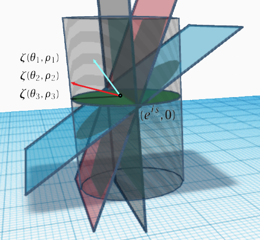
Figure 2: $R^{*}g(e^{is},0)$ integrates the function $g$ over all sets $E_{\zeta(\theta,\rho)}$ containing the point $(e^{is},0)$

Assuming $g$ is a well-behaved function, we can recover the original function $g$ from its mean values $R^{*}g$. We will first compute the forward equation $R^{*}g=h$ in terms of the Fourier coefficients of $R^{*}g$ and $g$. Once we have this expression, and noting the relationship between the Fourier coefficients of $R^{*}g$ and the right-sided Chebyshev fractional integrals, we will state conditions on $g$ for which $R^{*}g=h$ can be inverted.

Lemma 5.3.

Let $g\in C(\mathbb{S}^{2})$ be an even function and

$$g(\theta,\rho)=\sum_{n\in\mathbb{Z}}G_{n}(\rho)e^{in\theta}$$

its Fourier series representation for all $(\theta,\rho)\in\Xi$. Let $R^{*}g(e^{is},t)=\sum_{n\in\mathbb{Z}}H_{n}(t)e^{ins}$ be the Fourier series representation of $R^{*}g$ on $\mathbb{S}\times\mathbb{R}$. Then, for all $n\in\mathbb{Z}$

(19) $$H_{n}(t) =\frac{(-1)^{|n|}}{\sqrt{\pi}}\left(\Upsilon_{-}^{|n|}G_{n}^{\#}\right)(t)$$

where $\Upsilon_{-}^{|n|}$ is the right-sided Chebyshev fractional integral of order $|n|$ in Eq. 5 in Section 3 and

$$G_{n}^{\#}(v)=\frac{G_{n}\left(\arctan v\right)}{(1+v^{2})^{\frac{3}{2}}}.$$

Proof 5.4.

If $n\in\mathbb{Z}$, then using the formula for $R^{*}$ from Theorem 5.1

$$H_{n}(t)=\frac{1}{2\pi}\int_{0}^{2\pi}R^{*}g(e^{is},t)e^{-ins}\,ds$$

$$\qquad=\frac{1}{2\pi^{2}}\sum_{\sigma=\pm 1}\int_{0}^{2\pi}\,\int^{\infty}_{0}g\left(s+\sigma\arccos\left(\frac{-t}{\sqrt{v^{2}+t^{2}}}\right),\arctan\sqrt{v^{2}+t^{2}}\right)\,\frac{e^{-ins}dv\,ds}{(1+v^{2}+t^{2})^{\frac{3}{2}}}$$

$$\qquad=\frac{1}{2\pi^{2}}\sum_{\sigma=\pm 1}\int^{\infty}_{0}\,\int_{0}^{2\pi}g\left(s+\sigma\arccos\left(\frac{-t}{\sqrt{v^{2}+t^{2}}}\right),\arctan\sqrt{v^{2}+t^{2}}\right)\,\frac{e^{-ins}ds\,dv}{(1+v^{2}+t^{2})^{\frac{3}{2}}}.$$

Letting $u=s+\sigma\arccos\left(\frac{-t}{\sqrt{v^{2}+t^{2}}}\right)$ with respect to the $s$ variable and noting that the integrand is a $2\pi-$periodic function of $u$ yields

$$H_{n}(t) =\frac{1}{2\pi^{2}}\sum_{\sigma=\pm 1}\int^{\infty}_{0}\,\int_{0}^{2\pi}g\left(u,\arctan\sqrt{v^{2}+t^{2}}\right)\,\frac{e^{-in\left(u-\sigma\arccos\left(\frac{-t}{\sqrt{v^{2}+t^{2}}}\right)\right)}du\,dv}{(1+v^{2}+t^{2})^{\frac{3}{2}}}.$$

This way,

$$H_{n}(t) =\frac{1}{\pi}\sum_{\sigma=\pm 1}\int^{\infty}_{0}\left(\frac{1}{2\pi}\int_{0}^{2\pi}g\left(u,\arctan\sqrt{v^{2}+t^{2}}\right)e^{-inu}\,du\right)\,\frac{e^{in\sigma\arccos\left(\frac{-t}{\sqrt{v^{2}+t^{2}}}\right)}\,dv}{(1+v^{2}+t^{2})^{\frac{3}{2}}}$$

$$=\frac{1}{\pi}\sum_{\sigma=\pm 1}\int^{\infty}_{0}G_{n}\left(\arctan\sqrt{v^{2}+t^{2}}\right)\,\frac{e^{in\sigma\arccos\left(\frac{-t}{\sqrt{v^{2}+t^{2}}}\right)}\,dv}{(1+v^{2}+t^{2})^{\frac{3}{2}}}.$$

Using Euler’s formula and noticing that

$$\sin\left(n\sigma\arccos\left(\frac{-t}{\sqrt{v^{2}+t^{2}}}\right)\right) =\sigma\sin\left(n\arccos\left(\frac{-t}{\sqrt{v^{2}+t^{2}}}\right)\right)$$

$$\cos\left(n\sigma\arccos\left(\frac{-t}{\sqrt{v^{2}+t^{2}}}\right)\right) =\cos\left(n\arccos\left(\frac{-t}{\sqrt{v^{2}+t^{2}}}\right)\right)$$

yields

$$H_{n}(t) =(-1)^{|n|}\frac{2}{\pi}\int^{\infty}_{0}G_{n}\left(\arctan\sqrt{v^{2}+t^{2}}\right)\,\frac{T_{|n|}\left(\frac{t}{\sqrt{v^{2}+t^{2}}}\right)}{(1+v^{2}+t^{2})^{\frac{3}{2}}}\,dv$$

Letting $u=\arctan{\sqrt{v^{2}+t^{2}}}$ we obtain

$$H_{n}(t) =(-1)^{|n|}\frac{2}{\pi}\int_{\arctan|t|}^{\frac{\pi}{2}}G_{n}(u)\frac{T_{|n|}\left(\frac{t}{\tan u}\right)\tan u}{\sqrt{1+\tan^{2}u}\sqrt{\tan^{2}u-t^{2}}}\,du.$$

Making the change of variables $\omega=\tan u$ yields

$$H_{n}(t) =(-1)^{|n|}\frac{2}{\pi}\int_{|t|}^{\infty}G_{n}(\arctan\omega)\frac{\omega}{(1+\omega^{2})^{\frac{3}{2}}\sqrt{\omega^{2}-t^{2}}}T_{|n|}\left(\frac{t}{\omega}\right)\,d\omega.$$

Letting

(20) $$G_{n}^{\#}(\omega)=\frac{G_{n}\left(\arctan\omega\right)}{(1+\omega^{2})^{\frac{3}{2}}},$$

we can see that

$$H_{n}(t) =\frac{(-1)^{|n|}}{\sqrt{\pi}}\left(\Upsilon_{-}^{|n|}G_{n}^{\#}\right)(t),$$

where $\Upsilon_{-}^{|n|}$ is the right-sided Chebyshev fractional integral as defined in Eq. 5 in Section 3.

Null Space, Injectivity of $\mathbf{R}^{*}$ and an Inversion Formula

We will show that if a nontrivial, even, and continuous function $g$ belongs to the null space of $R^{*}$, then $g$ would be unbounded on the equator or at the poles of $\mathbb{S}^{2}$. This contradiction implies that $R^{*}$ is injective in the space of continuous and even functions on $\mathbb{S}^{2}$.

Now,

$$R^{*}g(e^{is},t)=0 \iff\forall n\in\mathbb{Z}\quad H_{n}(t)=0$$

$$\iff\forall n\in\mathbb{Z}\quad\frac{(-1)^{|n|}}{\sqrt{\pi}}\left(\Upsilon_{-}^{|n|}G_{n}^{\#}\right)(t)=0.$$

Assuming $G^{\#}_{n}$ fulfills the hypotheses in Lemma 3.6 and Lemma 3.8 and $R^{*}g=0$, then, by the aforementioned theorems, if $|n|<2$ then $G_{n}^{\#}=0$, implying that

$$G_{n}(\rho)=0$$

for all $\rho\in(0,\pi/2)$. If $|n|\geq 2$, then

$$G_{n}^{\#}(\omega)=\sum_{k=0}^{\lfloor\frac{|n|}{2}\rfloor-1}c^{n}_{k}\omega^{2k-|n|}$$

for $\omega\in(0,\infty)$ and some coefficients $c^{n}_{k}\in\mathbb{C}$. Therefore,

$$G_{n}^{\#}(\omega)=\sum_{k=0}^{\lfloor\frac{|n|}{2}\rfloor-1}c^{n}_{k}\omega^{2k-|n|} \iff G_{n}(\arctan\omega)=\sum_{k=0}^{\lfloor\frac{|n|}{2}\rfloor-1}c^{n}_{k}\omega^{2k-|n|}\left(1+\omega^{2}\right)^{\frac{3}{2}}$$

$$\iff G_{n}(\rho)=\sum_{k=0}^{\lfloor\frac{|n|}{2}\rfloor-1}c^{n}_{k}\frac{\left(1+\tan^{2}\rho\right)^{\frac{3}{2}}}{\tan^{|n|-2k}\rho}$$

for $\rho\in(0,\frac{\pi}{2})$.

Theorem 5.5.

The dual transform $R^{*}$ is injective in $C_{e}(\mathbb{S}^{2})$.

Proof 5.6.

Let $g\in C(\mathbb{S}^{2})$ be an even function and, without loss of generality, assume $0<\rho<\pi/2$. As $g$ is a continuous function, its Fourier coefficients $G_{n}(\rho)$ are also continuous on $[0,\pi/2]$. We begin by showing that $G_{n}^{\#}\in L_{\chi^{-}_{|n|}}((0,\infty))$, that is $G_{n}^{\#}$ satisfies Eq. 9 in Section 3 for all $n\in\mathbb{Z}$. Let $n\in\mathbb{Z}$ and $a_{1}>0$. If $n$ is even then

$$\int_{a_{1}}^{\infty}\left|G_{n}^{\#}(v)\right|\,dv =\int_{a_{1}}^{\infty}\frac{G_{n}(\arctan v)}{(1+v^{2})^{\frac{3}{2}}}\,dv$$

$$=\int_{\arctan a_{1}}^{\frac{\pi}{2}}\frac{|G_{n}(u)|}{\sqrt{1+\tan^{2}u}}\,du$$

by letting $u=\arctan v$. Therefore,

$$\int_{a_{1}}^{\infty}\left|G_{n}^{\#}(v)\right|\,dv \leq\int_{\arctan a_{1}}^{\frac{\pi}{2}}\left|G_{n}(u)\right|\,du$$

$$\leq\|G_{n}\|_{1}$$

$$<\infty.$$

If $n$ is odd then

$$\int_{a_{1}}^{\infty}\frac{\left|G_{n}^{\#}(v)\right|(1+|\log v|)}{v}\,dv =\int_{a_{1}}^{\infty}\frac{|G_{n}(\arctan v)|(1+|\log v|)}{v(1+v^{2})^{\frac{3}{2}}}dv$$

$$=\int_{\arctan a_{1}}^{\frac{\pi}{2}}\frac{|G_{n}(u)|(1+|\log\tan u|)}{\tan u\,\sqrt{1+\tan^{2}u}}du$$

by letting $u=\arctan v$. This way

$$\int_{a_{1}}^{\infty}\frac{\left|G_{n}^{\#}(v)\right|(1+|\log v|)}{v}\,dv \leq\int_{\arctan a_{1}}^{\frac{\pi}{2}}|G_{n}(u)|\frac{(1+|\log\tan u|)}{\tan u}du.$$

The quantity $\frac{(1+|\log\tan u|)}{\tan u}$ attains the following maximum in $[\arctan a_{1},\pi/2)$:

$$\max_{[\arctan a_{1},\pi/2)}\left\{\frac{(1+|\log\tan u|)}{\tan u}\right\}=\begin{cases}\frac{1}{a_{1}}+\frac{|\log a_{1}|}{a_{1}}&\quad\text{ if }0<a_{1}<1,\\ \frac{1}{a_{1}}+\frac{1}{e}&\quad\text{ if }1\leq a_{1}.\end{cases}$$

Therefore,

$$\int_{a_{1}}^{\infty}\frac{\left|G_{n}^{\#}(v)\right|(1+|\log v|)}{v}\,dv \leq\left(\frac{1}{a_{1}}+\max\left\{\frac{1}{e},\frac{|\log a_{1}|}{a_{1}}\right\}\right)\int_{\arctan a_{1}}^{\frac{\pi}{2}}|G_{n}(u)|du$$

$$\leq\left(\frac{1}{a_{1}}+\max\left\{\frac{1}{e},\frac{|\log a_{1}|}{a_{1}}\right\}\right)\|G_{n}\|_{1}$$

$$<\infty.$$

Thus proving that $G_{n}^{\#}\in L_{\chi^{-}_{|n|}}^{1}(0,\infty)$.

However, even and continuous functions in the null space of $R^{*}$ have Fourier series coefficients

$$G_{n}(\rho)\stackrel{{\scriptstyle\mathclap{\mbox{\small a.e.}}}}{{\quad=\quad}}\sum_{k=0}^{\lfloor\frac{|n|}{2}\rfloor-1}c^{n}_{k}\frac{\left(1+\tan^{2}\rho\right)^{\frac{3}{2}}}{\tan^{|n|-2k}\rho}$$

for all $|n|\geq 2$. Consequently, if any of the coefficients $c^{n}_{k}\neq 0$, then $g$ would not be continuous on the equator or at the poles of $\mathbb{S}^{2}$. It follows, that $R^{*}$ must have a trivial null space when defined in the space of continuous and even functions on $\mathbb{S}^{2}$.

Corollary 5.7.

The dual transform $R^{*}$ is injective in $R(H^{2}_{pc}(\mathbb{S}\times\mathbb{R}))$.

Proof 5.8.

Let $f\in H_{pc}^{2}(\mathbb{S}\times\mathbb{R})$. Since $R$ annihilates odd functions we may assume, without loss of generality, that $f$ is even. By Theorem 3.2 there exists a bounded and continuous function that is equal to $f$ almost everywhere. We may assume, without loss of generality, that $f$ denotes this continuous representative. Since $f$ is a continuous even function, $Rf$ is continuous and even on $\mathbb{S}^{2}$. Therefore, by Theorem 5.5, $R^{*}$ is injective in $R(H^{2}_{pc}(\mathbb{S}\times\mathbb{R}))$.

We conclude by providing an inversion formula.

Theorem 5.9.

Let $\Xi$ be as defined in Section 2, $g\in C(\overline{\Xi})$ be an even function on $\mathbb{S}^{2}$ and

$$g(\theta,\rho)=\sum_{n\in\mathbb{Z}}G_{n}(\rho)e^{in\theta}$$

its Fourier series representation for all $(\theta,\rho)\in\Xi$. If for $|n|\geq 2$

$$\int_{\arctan a}^{\frac{\pi}{2}}|G_{n}(u)|\tan^{|n|-1}u\,du<\infty\qquad\text{ for all a > 0},$$

then for almost all $t\in(0,\infty)$

$$G_{n}(\arctan t)=\begin{cases}\sqrt{\pi}(1+t^{2})^{\frac{3}{2}}\left(\textsc{D}^{\frac{1}{2}}_{-,2}H_{0}\right)(t)&\qquad\text{ for }n=0,\\ &\\ -\sqrt{\pi}t(1+t^{2})^{\frac{3}{2}}\left(D_{-,2}^{\frac{1}{2}}\frac{H_{1}}{t}\right)(t)&\qquad\text{ for }|n|=1,\\ &\\ (-1)^{|n|+1}\frac{\sqrt{\pi}}{2}(1+t^{2})^{\frac{3}{2}}\frac{d}{dt}\left(\overset{*}{\Upsilon}^{|n|}_{-}t^{-2}H_{n}\right)(t)&\qquad\text{ for }|n|\geq 2,\end{cases}$$

where

$$H_{n}(t) =\frac{(-1)^{|n|}}{\sqrt{\pi}}\left(\Upsilon_{-}^{|n|}G_{n}^{\#}\right)(t),$$

and

$$\textsc{D}^{\frac{1}{2}}_{-,2}\varphi =-\frac{1}{2}\frac{d}{dt}tI^{\frac{1}{2}}_{-,2}t^{-2}\varphi,$$

$$\left(I^{\frac{1}{2}}_{-,2}\varphi\right)(t) =\frac{2}{\sqrt{\pi}}\int_{t}^{\infty}\frac{\varphi(r)r}{\sqrt{r^{2}-t^{2}}}dr,$$

$$\left(\overset{*}{\Upsilon}^{m}_{-}\varphi\right)(t) =\frac{2t}{\sqrt{\pi}}\int_{t}^{\infty}\frac{\varphi(r)T_{m}\left(\frac{r}{t}\right)}{r\,\sqrt{r^{2}-t^{2}}}dr$$

as defined in Section 3.

Proof 5.10.

We prove this using Theorem 3.10 and Theorem 3.11 from Section 3. First notice that if $|n|<2$ the conditions of the aforementioned theorems imply that $g$ must be such that

$$\int_{\arctan a}^{\frac{\pi}{2}}\frac{|G_{n}(u)|\tan^{-\nu}u}{\sqrt{1+\tan^{2}u}}du<\infty\quad\text{ for all }a>0\text{ and }\nu=\begin{cases}0&\quad\text{ if }n\text{ is even}\\ 1&\quad\text{ if }n\text{ is odd.}\end{cases}$$

However, since $g$ is a continuous function on $\mathbb{S}^{2}$

$$\int_{\arctan a}^{\frac{\pi}{2}}\frac{|G_{n}(u)|\tan^{-\nu}u}{\sqrt{1+\tan^{2}u}}du \int_{\arctan a}^{\frac{\pi}{2}}|G_{n}(u)|\tan^{-\nu}u\,du$$

$$\leq\max\left\{\frac{1}{a},1\right\}\,\|G_{n}(u)\|_{1}$$

$$<\infty.$$

Therefore, since for $|n|<2$ we have that

$$\int_{\arctan a}^{\frac{\pi}{2}}\frac{|G_{n}(u)|(\tan u)^{-\nu}}{\sqrt{1+\tan^{2}u}}du<\infty\quad\text{ where }\nu=\begin{cases}0&\quad\text{ if }n\text{ is even}\\ 1&\quad\text{ if }n\text{ is odd,}\end{cases}$$

and

$$\int_{\arctan a}^{\frac{\pi}{2}}\frac{|G_{n}(u)|\tan^{|n|-1}u}{\sqrt{1+\tan^{2}u}}du \leq\int_{\arctan a}^{\frac{\pi}{2}}|G_{n}(u)|\tan^{|n|-1}u\,du$$

$$<\infty$$

for $|n|\geq 2$ and all $a>0$, by Theorem 3.10 and Theorem 3.11 $G_{n}(t)$ can be uniquely reconstructed almost everywhere from the mean values

(21) $$H_{n}(t) =\frac{(-1)^{|n|}}{\sqrt{\pi}}\left(\Upsilon_{-}^{|n|}G_{n}^{\#}\right)(t).$$

Moreover,

$$G_{n}(\arctan t)=\begin{cases}\sqrt{\pi}(1+t^{2})^{\frac{3}{2}}\left(\textsc{D}^{\frac{1}{2}}_{-,2}H_{0}\right)(t)&\qquad\text{ for }n=0,\\ &\\ -\sqrt{\pi}t(1+t^{2})^{\frac{3}{2}}\left(D_{-,2}^{\frac{1}{2}}\frac{H_{1}}{t}\right)(t)&\qquad\text{ for }|n|=1,\\ &\\ (-1)^{|n|+1}\frac{\sqrt{\pi}}{2}(1+t^{2})^{\frac{3}{2}}\frac{d}{dt}\left(\overset{*}{\Upsilon}^{|n|}_{-}t^{-2}H_{n}\right)(t)&\qquad\text{ for }|n|\geq 2,\end{cases}$$

We would like to point out that, analogously to Remark 2.53 from [15], we may relax the assumptions on $G_{n}$ for $|n|\geq 2$ by assuming only that $g$ is a continuous function on $\mathbb{S}^{2}$. In this case, we can find non-unique solutions to the forward equation

$$H_{n}(t) =\frac{(-1)^{|n|}}{\sqrt{\pi}}\left(\Upsilon_{-}^{|n|}G_{n}^{\#}\right)(t)$$

for all $|n|\geq 2$.