Chromoelectric and chromomagnetic correlators at high temperature from gradient flow

Abstract

The heavy quark diffusion coefficient is encoded in the spectral functions of the chromoelectric and the chromomagnetic correlators that are calculable on the lattice. We study the chromoelectric and the chromomagnetic correlator in the deconfined phase of SU(3) gauge theory using Symanzik flow at two temperatures $1.5T_{c}$ and $10000T_{c}$, with $T_{c}$ being the phase transition temperature. To control the lattice discretization errors and perform the continuum limit we use several temporal lattice extents $N_{t}=16,20,24$ and 28. We observe that the flow time dependence of the chromomagnetic correlator is quite different from chromoelectric correlator most likely due to the anomalous dimension of the former as has been pointed out recently in the literature.

1 Introduction

The quark gluon plasma is an extreme state of matter at high temperatures, which can be probed in relativistic heavy ion collisions [1]. Measurements in heavy ion collisions are used to test the QCD phase diagram, which also gives important implications for cosmology and neutron stars. The interpretation of experimental data requires first principle QCD calculations. The heavy quark momentum diffusion coefficient is one of the quantities of interest and can be related to experimental observables such as nuclear suppression factor and elliptic flow of open heavy flavor hadrons. However, perturbative calculations of the heavy quark diffusion at LO [2, 3] and at NLO [4] lead to quite different results, suggesting that these calculations are not reliable. Hence, non-perturbative calculations are needed.

The heavy quark diffusion coefficient has been defined through the correlator of two chromoelectric fields [5]. Using nonrelativistic effective field theories and open quantum systems, the same object emerges in the description of quarkonium evolution in medium [6]. Previous lattice calculations of this object [7, 8, 9, 10, 11] were performed in quenched QCD and the heavy quark diffusion constant is obtained as the intercept of the chromolectric correlator spectral function at zero frequency [4]. The chromoelectric correlator is very noisy and to reduce the noise the multi-level algorithm has been used in the above studies. Recently, it has been suggested to use the gradient flow as an alternative noise reduction method and this approach turned out to be successful in calculating the heavy quark diffusion coefficient at $1.5T_{c}$ [12]. Furthermore, in Ref. [13] the $1/M$ effects in heavy quark diffusion were considered, with $M$ being the heavy quark mass. These effects are encoded in the chromomagnetic correlator [13]. In this contribution we will present numerical lattice calculations of the chromoelectric and chromomagnetic correlators at temperatures of $1.5T_{c}$ and $10^{4}T_{c}$. We will use the gradient flow method for noise reduction which also ensures the non-perturbative renormalization.

2 Physical Background

Within a quark gluon plasma heavy quarks can diffuse through the medium. Thereby, the heavy quark momentum is changed by random kicks from the medium which can be described by a Brownian motion encoded into the Langevin dynamics

$$\dot{\mathbf{p}}-\eta\mathbf{p} =\mathbf{f}(t),$$ (1)

where $\dot{\mathbf{p}}$ is the temporal derivative of the heavy quark momentum $\mathbf{p}$, $\eta$ is the drag coefficient, and $\mathbf{f}$ is the random force acting on the heavy quark that satisfies

$$\langle f_{i}(t)\rangle =0,\ \langle f_{i}(t^{\prime})f_{j}(t)\rangle=\kappa\delta_{ij}\delta(t-t^{\prime}),$$ (2)

where $\kappa$ is the heavy quark momentum diffusion coefficient. The drag coefficient and the heavy quark momentum diffusion coefficient are connected through the Einstein equation, which after including the leading relativistic correction reads [13]

$$\eta\approx\frac{\kappa}{2MT}\left(1-\frac{5T}{2M}\right),$$ (3)

where $T$ is the temperature and $M$ the mass of the heavy quark.

As mentioned above, the heavy quark diffusion coefficient can be obtained from the Euclidean chromoelectric correlator [5, 4] and the chromomagnetic correlator [13]

$$G_{E}(\tau) =-\frac{1}{3}\frac{\sum_{i}\mathrm{Tr}\langle U(\beta;\tau)gE_{i}(\tau)U(\tau;0)gE_{i}(0)\rangle}{\mathrm{Tr}\langle U(\beta;0)\rangle}$$ (4)

$$G_{B}(\tau) =\frac{1}{3}\frac{\sum_{i}\mathrm{Tr}\langle U(\beta;\tau)gB_{i}(\tau)U(\tau;0)gB_{i}(0)\rangle}{3\mathrm{Tr}\langle U(\beta;0)\rangle},$$ (5)

where $\tau$ is the temporal separation of the field insertions and $E_{i}$ and $B_{i}$ are the chromoelectric and chromomagnetic field respectively. The Wilson lines $U(\tau;0)$ in the above expression are in the fundamental representation and wrap around the periodic boundary making the correlators gauge invariant. The denominator cancels out the self energy divergence in the above expression. The chromoelectric correlator defined above also plays an important role in quarkonium suppression [6].

The chromoelectric and chromomagnetic correlators are connected to the respective diffusion coefficient $\kappa_{E/B}$ through the spectral function

$$G_{E/B}(\tau)=\int_{0}^{\infty}\frac{\mathrm{d}\omega}{\pi}\rho_{E/B}(\omega)\frac{\cosh\left(\frac{\beta}{2}-\tau\right)\omega}{\sinh\frac{\beta\omega}{2}},\ \ \ \ \kappa_{E/B}=\lim_{\omega\rightarrow 0}\frac{2T\rho_{E/B}(\omega)}{\omega}.$$ (6)

The spectral functions $\rho_{E/B}$ are known perturbatively, see Ref. [14] for $\rho_{E}$ at NLO and [13] for $\rho_{B}$ at LO. The total heavy quark momentum diffusion coefficient results into

$$\kappa\approx\kappa_{E}+\frac{2}{3}\langle\mathbf{v}^{2}\rangle\kappa_{B},$$ (7)

where $\langle\mathbf{v}^{2}\rangle\sim T/M$ is the velocity of the heavy quark [13]. Therefore, the chromoelectric correlator contributes in the leading order of the heavy quark mass and the chromomagnetic correlator in the first order correction, since $\langle\mathbf{v}^{2}\rangle$ is of order $T/M$ [13]. In Ref. [14] $\kappa_{E}$ is determined up to LO and in Ref. [13] $\kappa_{B}$, where the LO of $\kappa_{E}$ starts at $\mathcal{O}(g^{2})$ and the LO of $\kappa_{B}$ at $\mathcal{O}(g^{4})$.

3 Implementation and results

On the lattice the chromoelectric and magnetic fields need to be discretized. For the chromoelectric field we use [15]

$$E_{i}(\tau,\mathbf{x})=U_{i}(\tau,\mathbf{x})U_{4}(\tau,\mathbf{x}+a\hat{\mathbf{e}_{i}})-U_{4}(\tau,\mathbf{x})U_{i}(\tau,\mathbf{x}+a\hat{\mathbf{e}}_{4}),$$ (8)

where $U_{\mu}(\tau,\mathbf{x})$ is the link variable with lattice spacing $a$. Similarly, we use the following discretization for $B$-field

$$B_{i}(\tau,\mathbf{x})=\epsilon_{ijk}U_{j}(\tau,\mathbf{x})U_{k}(\tau,\mathbf{x}+a\hat{\mathbf{e}}_{j}),$$ (9)

where we now obtain a loop within the spatial plane which lies perpendicularly to the spatial direction $i$ of the $B_{i}$-field component. By expanding the link variables in a small lattice spacing in Eq. (9) it can be shown that the discretized $B$-field corresponds to the chromomagnetic components of the field strength tensor at leading order.

The chromoelectric correlator calculated on the lattice needs to be renormalized [16]. For the chromomagnetic correlator, renormalization is needed even in the continuum theory [17]. Since gradient flow renormalizes gauge invariant observables automatically [18], no renormalization is needed for measurements at finite flow time.

$N_{s}$	$N_{t}$	$\beta$	$N_{\mathrm{conf}}$
48	16	6.872	990
48	20	7.044	3660
48	24	7.192	4200
56	28	7.321	4080

(a) $T=1.5T_{c}$

$N_{s}$	$N_{t}$	$\beta$	$N_{\mathrm{conf}}$
48	16	14.443	990
48	20	14.635	990
48	24	14.792	1500
56	28	14.925	1950

(b) $T=10^{4}T_{c}$

Table 1: The lattice parameters used in our calculations for $1.5T_{c}$ and $10^{4}T_{c}$. Here $T_{c}$ is the critical temperature.

In this study we focus on two temperatures $1.5T_{c}$ and $10^{4}T_{c}$ on quenched lattices as listed in table 1. Here the critical temperature $T_{c}$ and the temperature values are determined using the scale setting procedure of Ref. [19]. The ensembles are generated with Wilson gauge action using the heatbath and overrelaxation algorithm. We compute the field correlators using the gradient flow algorithm [18, 20] with Symanzik action. In order to obtain a dimensionless and tree level improved quantity we normalize the final measured correlator values with the leading order lattice correlator [12] at zero flow time

$$G^{\scriptscriptstyle\text{norm}}=\frac{G^{\begin{subarray}{c}\scriptscriptstyle\text{LO}\\ \scriptscriptstyle\text{latt}\end{subarray}}(\tau,\tau_{F}=0)}{g^{2}C_{F}},$$ (10)

where $\tau_{F}$ is the finite flow time. We assume the leading order of the chromoelectric and magnetic correlators to be the same. We obtain a tree level improved quantity by using the perturbative lattice correlator as normalization instead of the perturbative continuum correlator.

The final renormalized values of the correlators are obtained in a zero flow time limit. However, the zero flow time limit can only be taken after the continuum extrapolation is performed. Therefore, we calculate the correlators at different lattice spacings and then perform the continuum extrapolation. Afterwards, we can perform the zero flow time limit.

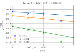
Figure 1: Examples for the continuum limits of the chromoelectric and chromomagnetic correlators at four different flow times at $T=1.5T_{c}$.

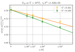
Figure 2: Examples for the continuum limits of the chromoelectric and chromomagnetic correlators at four different flow times at $T=10^{4}T_{c}$.

To obtain the continuum limit, we interpolate the data in $\tau T$ with cubic splines, using natural boundary conditions at $\tau T=0$ (second derivative equal to zero) and symmetric boundary conditions at $\tau T=0.5$ (first derivative equal to zero) in order to have data of the same $\tau T$ axis on all lattices, and perform linear extrapolations over $1/N_{t}^{2}$ to the continuum ($N_{t}\rightarrow\infty$) using lattices with temporal extents of $N_{t}=20,24,28$. Figs. 1 and 2 show some typical examples of continuum extrapolations for the chromoelectric and magnetic fields respectively. In these figures, we also show the $N_{t}=16$ data points. It appears that the $N_{t}=16$ data are not in $1/N_{t}^{2}$ scaling regime. Therefore, we do not include these in the continuum extrapolations. We expect the spatial size dependence to be negligible [11].

Figure 3: The final results of the continuum limit for the chromoelectric and magnetic correlators at $T=1.5T_{c}$.

In Fig. 3 we show the continuum extrapolated results for $T=1.5T_{c}$. For the chromoelectric correlator we perform a linear extrapolation in $\tau_{F}T^{2}$, which is also shown in Fig. 3. When performing the extrapolation we considered flow time $\tau_{F}$ in a restricted range

$$a\leq\sqrt{8\tau_{F}}\leq\frac{\tau-a}{3}.$$ (11)

Here $\sqrt{8\tau_{F}}$ is often called the flow radius. The above constrain for the flow time comes from the fact that for this range the perturbative flowed correlator deviates less than $1\text{\,}\mathrm{\char 37\relax}$ from the unflowed correlator [12]. For larger flow times the dependence on $\tau_{F}T^{2}$ is nonlinear and the corresponding data cannot be used for the $\tau_{F}\rightarrow 0$ extrapolations. It is obvious from Fig. 3 that the flow time dependence of the chromoelectric and chromomagnetic correlators is quite different. It remains to bee seen if this difference in the flow time dependence is related to the anomalous dimension of the chromomagnetic correlator [17].

Figure 4: The final results of the continuum limit for the chromoelectric and magnetic correlators at $T=10^{4}T_{c}$.

Fig. 4 shows the final results of the continuum limits at $T=10^{4}T_{c}$. We perform the same zero flow time procedure as for the $T=1.5T_{c}$ case as indicated in Fig. 4. We obtain the same flow time behaviour of the correlators for $\tau_{F}\rightarrow 0$.

Figure 5: Final results on $G_{E}$ in the limit of zero flow time compared with previous results [12] based on gradient flow and on the calculations with multilevel algorithm [11].

In Fig. 5 we show the final results for the chromoelectric correlator as function of $\tau$ in the zero flow time limit. Our results are compared with results from Ref. [12] at $T=1.5T_{c}$, which also rely on gradient flow, and with results from Ref. [11], which are calculated with a multilevel approach at $T=1.5T_{c}$ and $T=10^{4}T_{c}$. The multilevel results are renormalized by the 1-loop renormalization constant from Ref. [16]. We see that our results agree with the previous calculations at both temperatures, hence, we can conclude that the gradient flow approach serves as a non-perturbative renormalization method.

Figure 6: The chromomagnetic correlator as function of $\tau$ obtained for different flow times, $\tau_{F}$.

For the chromomagnetic correlator the zero flow time limit cannot be taken because of the anomalous dimension [17]. Therefore, in Fig. 6 we show the chromomagnetic correlator for four different flow times. We see that $G_{B}$ is almost $\tau_{F}$-independent for $\tau T\geq 0.25$ at $T=1.5T_{c}$. For $T=10^{4}T_{c}$ the chromomagnetic correlator is roughly flow time independent for $\tau T\geq 0.3$.

4 Conclusions

In this contribution we studied the chromoelectric and chromomagnetic correlators in quenched QCD at two temperatures, $1.5T_{c}$ and $10^{4}T_{c}$. These correlators are interesting as they encode information on the heavy quark diffusion coefficient. We used the gradient flow to reduce the noise in the lattice calculations of these correlators as well as to obtain the renormalized results. We have found that the flow time dependence of the chromoelectric and chromomagnetic correlators is quite different for small flow times. For the chromoelectric correlator we performed the zero flow time extrapolation and found that for both temperatures the zero flow time extrapolated results agree with the previously published ones.

References

- [1] R. Pasechnik and M. Šumbera, Phenomenological Review on Quark–Gluon Plasma: Concepts vs. Observations, Universe 3 (2017) 7 [1611.01533].
- [2] G.D. Moore and D. Teaney, How much do heavy quarks thermalize in a heavy ion collision?, Phys. Rev. C 71 (2005) 064904 [hep-ph/0412346].
- [3] B. Svetitsky, Diffusion of charmed quarks in the quark-gluon plasma, Phys. Rev. D 37 (1988) 2484.
- [4] S. Caron-Huot and G.D. Moore, Heavy quark diffusion in QCD and N=4 SYM at next-to-leading order, JHEP 02 (2008) 081 [0801.2173].
- [5] J. Casalderrey-Solana and D. Teaney, Heavy quark diffusion in strongly coupled N=4 Yang-Mills, Phys. Rev. D 74 (2006) 085012 [hep-ph/0605199].
- [6] N. Brambilla, M.A. Escobedo, J. Soto and A. Vairo, Heavy quarkonium suppression in a fireball, Phys. Rev. D 97 (2018) 074009 [1711.04515].
- [7] H.B. Meyer, The errant life of a heavy quark in the quark-gluon plasma, New J. Phys. 13 (2011) 035008 [1012.0234].
- [8] A. Francis, O. Kaczmarek, M. Laine and J. Langelage, Towards a non-perturbative measurement of the heavy quark momentum diffusion coefficient, PoS LATTICE2011 (2011) 202 [1109.3941].
- [9] D. Banerjee, S. Datta, R. Gavai and P. Majumdar, Heavy Quark Momentum Diffusion Coefficient from Lattice QCD, Phys. Rev. D 85 (2012) 014510 [1109.5738].
- [10] A. Francis, O. Kaczmarek, M. Laine, T. Neuhaus and H. Ohno, Nonperturbative estimate of the heavy quark momentum diffusion coefficient, Phys. Rev. D 92 (2015) 116003 [1508.04543].
- [11] N. Brambilla, V. Leino, P. Petreczky and A. Vairo, Lattice QCD constraints on the heavy quark diffusion coefficient, Phys. Rev. D 102 (2020) 074503 [2007.10078].
- [12] L. Altenkort, A.M. Eller, O. Kaczmarek, L. Mazur, G.D. Moore and H.-T. Shu, Heavy quark momentum diffusion from the lattice using gradient flow, Phys. Rev. D 103 (2021) 014511 [2009.13553].
- [13] A. Bouttefeux and M. Laine, Mass-suppressed effects in heavy quark diffusion, JHEP 12 (2020) 150 [2010.07316].
- [14] Y. Burnier, M. Laine, J. Langelage and L. Mether, Colour-electric spectral function at next-to-leading order, JHEP 08 (2010) 094 [1006.0867].
- [15] S. Caron-Huot, M. Laine and G.D. Moore, A Way to estimate the heavy quark thermalization rate from the lattice, JHEP 04 (2009) 053 [0901.1195].
- [16] C. Christensen and M. Laine, Perturbative renormalization of the electric field correlator, Phys. Lett. B 755 (2016) 316 [1601.01573].
- [17] M. Laine, 1-loop matching of a thermal Lorentz force, JHEP 06 (2021) 139 [2103.14270].
- [18] M. Lüscher, Properties and uses of the Wilson flow in lattice QCD, JHEP 08 (2010) 071 [1006.4518].
- [19] A. Francis, O. Kaczmarek, M. Laine, T. Neuhaus and H. Ohno, Critical point and scale setting in SU(3) plasma: An update, Phys. Rev. D 91 (2015) 096002 [1503.05652].
- [20] A. Bazavov and T. Chuna, Efficient integration of gradient flow in lattice gauge theory and properties of low-storage commutator-free Lie group methods, 2101.05320.