Max-algebraic hybrid automata: Modelling and equivalences

Abstract

This article introduces the novel framework of max-algebraic hybrid automata as a hybrid modelling language in the max-plus algebra. We show that the modelling framework unifies and extends the switching max-plus linear systems framework and is analogous to the discrete hybrid automata framework in conventional algebra. In addition, we show that the framework serves as a bridge between automata-theoretic models in max-plus algebra and switching max-plus linear systems. In doing so, we formalise the relationship between max-plus automata and switching max-plus linear systems in a behavioural sense. This also serves as another step towards importing tools for analysis and optimal control from conventional time-driven hybrid systems to discrete-event systems in max-plus algebra.

blue

1 Introduction

Max-algebraic models are particularly suited for modelling discrete-event systems, with synchronisation but no concurrency or choice, when timing constraints on event occurrences are of explicit concern in system dynamics and performance specifications [1, 2, 13]. The modelling class coincides with that of timed-event graphs. Moreover, the modelling formalism provides a continuous-variable dynamic representation of discrete-event systems analogously to time-driven systems. This similarity has served as the key motivation in the development of max-plus linear systems theory, analogously to classical linear systems theory [1, 4].

The major limitation of the max-plus linear modelling framework is rooted in its inability to model competition and/or conflict among several event occurrences [13]. The formalism then resorts to the dual min-plus operations to model conflict resolution policies explicitly in the algebraic system description [1, 3].

Automata-theoretic models for discrete-event systems, on the other hand, are particularly suited for modelling conflicts and certain forms of concurrency. To this end, models have been proposed in literature that follow a modular approach by allowing the conflict resolution mechanism be handled by a discrete variable taking values in a finite set [7, 23]. The resulting hybrid phenomenon due to the interaction of the discrete-valued and continuous-valued dynamics is the focus of this article. In this context, there are two layers of behaviour that are studied: logical ordering of the events on the one hand, and the timing of events on the other.

The max-plus automata approach for modelling the aforementioned hybrid phenomenon forms an extension of finite automata where transitions are given weights in the max-plus algebra [7]. The weight encodes the timing information as the price of taking the transition. The output under a given input sequence over an event alphabet is then evaluated, in the max-plus algebra, as the accumulated weight. Such models lend themselves to path-based performance analysis for discrete-event systems [7, 8].

An alternative approach involves the Switching Max-Plus Linear (SMPL) modelling paradigm [23]. Such models extend the max-plus linear modelling framework by allowing changes in the structure of synchronisation and ordering constraints as the system evolves [23]. This offers a compromise between the powerful description of hybrid systems and the decision-making capabilities in max-plus algebra [5, 23]. Moreover, the SMPL formalism offers the flexibility of explicitly modelling different switching mechanisms between the operating modes in a single framework [24].

In current article, we propose a novel max-algebraic hybrid automata framework to model discrete-event systems analogously to the hybrid automata framework of [15, 17] for conventional time-driven systems. In the proposed framework, the discrete-valued dynamics is represented as a labelled oriented graph and the continuous-valued dynamics is associated to each discrete state. We formally prove that this serves as a unifying framework for studying the aforementioned models and their equivalence relationships in the behavioural framework [27, 12, 26].

The paper is organised as follows. Section 2 gives some background on the max-plus algebra. Section 3 reviews the literature on discrete-event systems in max-plus algebra focusing on SMPL and max-plus automata frameworks. Section 4 introduces the unifying modelling framework of max-algebraic hybrid automata and its finite-state discrete abstraction. Section 5 establishes the relationships among different modelling classes namely, SMPL, max-plus automata, and the proposed max-algebraic hybrid automata. The paper ends with concluding remarks in Section 6.

2 Preliminaries

This section presents some basics in max-plus and automata theory based entirely on [1, 11, 19, 9, 6, 2].

The set of all positive integers up to $n$ is denoted as $\underline{n}=\{l\in\mathbb{N}\,|\,l\leq n\}$ where $\mathbb{N}=\{1,2,3,\dots\}$.

Max-plus algebra. The max-plus semiring, $\mathbb{R}_{\mathrm{max}}=(\mathbb{R}_{\varepsilon},\oplus,\otimes)$, consists of the set $\mathbb{R}_{\varepsilon}=\mathbb{R}\cup\{-\infty\}$ endowed with the addition $(a\oplus b=\mathrm{max}(a,b))$ and the multiplication $(a\otimes b=a+b)$ operations [1]. The zero element is denoted as $\varepsilon=-\infty$ and the unit element as $\mathds{1}=0$. These elements are identities with respect to $\oplus$ and $\otimes$, respectively, and $\varepsilon$ is absorbing for $\otimes$. However, the max-plus algebra lacks an additive inverse operation (since $a\oplus b=\varepsilon$ implies $a=b=\varepsilon$). The matrix with all entries $\varepsilon$ is denoted as $\mathcal{E}$. The max-plus powers of a matrix $A\in{\mathbb{R}}_{\varepsilon}^{n\times n}$ are defined recursively as ${A}^{{\scriptscriptstyle\otimes}^{\scriptstyle{k+1}}}={A}^{{\scriptscriptstyle\otimes}^{\scriptstyle{k}}}\otimes A$ for $k\in\mathbb{N}$. The partial order $\leq$ is defined such that for vectors $x,y\in\mathbb{R}^{n}_{\varepsilon}$, $x\leq y\Leftrightarrow x\oplus y=y\Leftrightarrow x_{i}\leq y_{i},\;\forall i\in\underline{n}$.

The max-plus vector and matrix operations can be defined analogously to the conventional algebra. Let $A,B\in\mathbb{R}^{m\times n}_{\varepsilon}$, and $C\in\mathbb{R}^{n\times p}_{\varepsilon}$; then

$$[A\oplus B]_{ij} =a_{ij}\oplus b_{ij}=\max\left(a_{ij},b_{ij}\right)$$

$$[A\otimes C]_{ij} =\bigoplus_{k=1}^{n}a_{ik}\otimes c_{kj}=\max_{k}\left(a_{ik}+c_{kj}\right)$$

where the $(i,j)$-th element of a matrix $A$ is denoted as $[A]_{ij}$ or $a_{ij}$. Likewise, the $i$-th element of a vector $x$ is denoted as $x_{i}$.

The min-plus semiring, $\mathbb{R}_{\mathrm{min}}=(\mathbb{R}_{\top},\oplus^{\prime},\otimes^{\prime})$ is defined as a dual of the max-plus semiring acting on the set $\mathbb{R}_{\top}=\mathbb{R}\cup\{+\infty\}$. The zero element is $\top=+\infty$. The vector and matrix operations are then defined analogously. The completed max-plus semiring is defined over the set $\overline{\mathbb{R}}_{\varepsilon}=\mathbb{R}_{\varepsilon}\cup\{\top\}$ such that max-plus operations take preference. The set of all vectors in $\overline{\mathbb{R}}^{n}_{\varepsilon}$ with at least one finite entry is denoted as $\overline{\mathbb{R}}^{n}_{\varepsilon}\setminus\{\varepsilon,\top\}^{n}$.

The max-plus Boolean semiring defined as $\mathbb{B}_{\max}=(\mathbb{B}_{\varepsilon},\oplus,\otimes)$, where $\mathbb{B}_{\varepsilon}=\{\varepsilon,\mathds{1}\}$, is isomorphic to the Boolean semiring $\mathbb{B}=(\{\mathrm{false},\mathrm{true}\},\mathrm{or},\mathrm{and})$.

Max-min-plus-scaling functions. The Max-Min-Plus-Scaling (MMPS) expression $f$ of the variables $x_{1},\dots,x_{n}$ is defined by the grammar

$$f:=x_{i}|\alpha|f_{k}\oplus f_{l}|f_{k}\oplus^{\prime}f_{l}|f_{k}+f_{l}|\beta\cdot f_{k},\;\alpha,\beta\in\mathbb{R},\;i\in\underline{n},$$ (1)

where $f_{k}$ and $f_{l}$ are again MMPS expressions.

A max-min-plus expression $f$ of variables $x_{1},\dots,x_{n}$ is defined by the grammar

$$f:=x_{i}|f_{k}\oplus f_{l}|f_{k}\oplus^{\prime}f_{l}|f_{k}+\alpha,\;\alpha\in\mathbb{R},\;i\in\underline{n},$$ (2)

where $f_{k}$ and $f_{l}$ are again max-min-plus expressions. Any such max-min-plus expression $f$ can be placed in the max-min-plus conjunctive form:

$$f =f_{1}\oplus^{\prime}f_{2}\oplus^{\prime}\cdots\oplus^{\prime}f_{m},$$ (3)

$$i \neq j\Rightarrow f_{i}\nleq f_{j},$$

where $f_{j}=(a_{j1}\otimes x_{1})\oplus(a_{j2}\otimes x_{2})\oplus\cdots\oplus(a_{jn}\otimes x_{n})$ is said to be a max-plus projection of $f$ with $a_{ji}\in\mathbb{R}_{\varepsilon}$ for all $i\in\underline{n}$ and $j\in\underline{m}$. The max-min-plus conjunctive form (3) is unique up to reordering of $f_{j}$’s [9, Theorem 2.1]. Note that the stated uniqueness is necessary for the definition of transition graphs (Definition 3 below).

Set theory. Let $P$ be a finite set. Then $|P|$, $2^{P}$, and $P^{*}$ denote the cardinality, power set (set of all subsets), and set of non-empty finite sequences of elements from $P$, respectively. A non-empty finite set of symbols is referred to as an alphabet. When a set $P$ is a countable collection of variables, the set of valuations of its variables is denoted as $\mathbb{P}$.

Finite automaton. A finite automaton is a tuple $\mathcal{T}=(Q,\Sigma,\delta,Q_{\mathrm{0}},Q_{\mathrm{f}})$ consisting of a finite set of states $Q$, a finite alphabet of inputs $\Sigma$, a partial transition function $\delta:Q\times\Sigma\to 2^{Q}$, a non-empty set of initial states $Q_{\mathrm{0}}\subseteq Q$, and a non-empty set of final states $Q_{\mathrm{f}}\subseteq Q$. A labelled transition is denoted as $q\xrightarrow[]{l}q^{\prime}$ for $q^{\prime}\in\delta(q,l)$, $l\in\Sigma$.

A finite word is defined as a sequence (concatenation) of inputs $\omega_{m}=l_{1}l_{2}\cdots l_{m}$. Here, $\omega_{m}=\omega_{m-1}l_{m}$, $l_{j}\in\Sigma$ for $j\in\underline{m}$. An empty word is denoted as $\epsilon$. An accepting path for a word $\omega_{m}\in\Sigma^{*}$ on the finite automaton $\mathcal{T}$ is defined as the sequence of states $(q_{0},q_{1},\dots,q_{m})\in Q^{m+1}$ if $q_{0}\in Q_{\mathrm{0}}$, $q_{m}\in Q_{\mathrm{f}}$, and $q_{i}\in\delta(q_{i-1},l_{i})$ for all $i\in\underline{m}$. The set of words $\omega_{m}\in\Sigma^{*}$, $m\in\mathbb{N}$ accepted by some path on the finite automaton is denoted as $\llbracket\mathcal{T}\rrbracket_{\mathrm{L}}$, i.e. the language of the finite automaton $\mathcal{T}$.

3 Max-algebraic models of discrete-event systems

This section aims at recapitulating models in the max-plus algebra that capture synchronisation as well as certain forms of concurrency in discrete-event systems. For simplification of the exposition and for further systematic comparisons, we also present a common description of the underlying signals in discrete-event systems.

3.1 Synchronisation and concurrency

The max-algebraic modelling paradigm characterises the behaviour of a discrete-event system by capturing the sequences of occurrence times of events (or, temporal evolution) over a discrete event counter. This, in particular, is useful when the events are ordered by the phenomena of synchronisation (max operation), competition (min operation), and time delay (plus operation) [1]. The phenomenon of concurrency arising due to variable sequencing (and hence variable synchronisation and ordering structure) of events can lead to a semi-cyclic behaviour [25]. Below we discuss two different modelling approaches, namely SMPL systems and max-plus automata, that extend the max-plus linear framework to incorporate such concurrency. Here, the shared characteristic is the introduction of a discrete variable that completely specifies the ordering structure at a given event counter. This interaction of synchronisation and concurrency is, thus, hybrid in nature.

3.2 Signals in discrete-event systems

We refer to variables with finite or countable valuations as discrete, and variables with valuations in $\overline{\mathbb{R}}_{\varepsilon}$ as continuous. An event-driven system with both continuous and discrete variables evolving over a discrete counter $k$ is characterised by the following signals:

• $x(\cdot)$ and $l(\cdot)$: continuous and discrete states respectively;

• $u(\cdot)$ and $v(\cdot)$: continuous and discrete controlled inputs respectively;

• $y(\cdot)$: continuous output;

• $r(\cdot)$ and $w(\cdot)$: continuous and discrete exogenous inputs respectively. The signal $r(\cdot)$ can represent a reference signal or a max-plus additive uncertainty in the continuous state $x$. The signal $w(\cdot)$ can represent a scheduling signal or uncertainty in mode switching;

• $p(\cdot)$: continuous exogenous signal. It can represent a parametric or max-plus multiplicative perturbation in the continuous dynamics that is either exogenous or state-dependent.

The uncontrolled exogenous inputs, hereafter, are collected into a single signal $\Theta(\cdot)$. This signal is partitioned as $\Theta=[\Theta_{\mathrm{x}}^{\top},\;\Theta_{\ell}^{\top}]^{\top}$. Here $\Theta_{\mathrm{x}}=[r^{\top},\;p^{\top}]^{\top}$ denotes the uncertainty in the continuous-state evolution, and $\Theta_{\ell}=w$ denotes the uncertainty in the discrete-state evolution.

3.3 Switching max-plus linear systems

The dynamics of a general model in max-plus algebra in mode $l(k)\in\mathcal{L}\triangleq\underline{n_{\mathrm{L}}}$ for the continuous state $x(k)\in\overline{\mathbb{R}}^{n}_{\varepsilon}$ at event counter $k\in\mathbb{N}$ can be written as follows:

$$x(k) =f(l(k),x(k-1),u(k),\Theta_{\mathrm{x}}(k)),$$ (4)

$$l(k) =\phi(l(k-1),x(k-1),u(k),v(k),\Theta_{\ell}(k)),$$

$$y(k) =h(l(k),x(k),u(k),\Theta_{\mathrm{x}}(k))$$

where the functions $f(\cdot)$ and $h(\cdot)$ represent the evolution of the continuous state and output, respectively, as MMPS functions. The function $\phi(\cdot)$ encodes the switching mechanism.

We refer to an open-loop SMPL system, $\mathcal{S}_{\mathrm{O}}$, when the functions $f$ and $g$ are max-plus linear in states and inputs for a fixed $l$ and control inputs $u$ and $v$ are absent. On the other hand, we refer to a controlled SMPL system, $\mathcal{S}_{\mathrm{C}}$, when a controller is also part of the system description. The control inputs in (4) can then be modelled as outputs of a control algorithm:

$$u(k) =f^{(u)}_{\mathrm{C}}(z(k),\Theta(k))$$ (5)

$$v(k) =f^{(v)}_{\mathrm{C}}(z(k),\Theta(k)).$$

Here, the signal $z(\cdot)$ denotes the performance signal composed of the (past) known values of the continuous and discrete states, and continuous inputs. It is noted here that the functions $f^{(\cdot)}_{\mathrm{C}}$ might not have a closed form. The most popular control algorithms for continuous-valued discrete-event systems in literature are residuation [18] and model predictive control [24].

An important subclass of controlled SMPL systems can be represented using max-min-plus linear functions. This encompasses the class of max-plus linear systems in open-loop and closed-loop with static [23] and certain dynamic feedback controllers (for e.g., via residuation [14]). The max-min-plus linear functions can also be used to model the dynamics of a subclass of timed Petri nets under a first-in first-out policy [19, 20].

A controlled SMPL system can be represented as the connection of an MMPS dynamics $f$ in (4) and a controller dynamics $f_{\mathrm{C}}$ in (5) via a switching mechanism $\phi$ in (4). The controlled SMPL system can then be represented as a modification of discrete hybrid automata proposed in [21] as shown in Fig. 1. The major differences between our framework and that of [21] are: i) the control algorithm is explicitly included in the model description, and ii) the mode selector can also model a discrete dynamic process. The mode dynamics, however, is still piecewise affine due to the equivalence of max-min-plus-scaling and piecewise-affine systems under fairly non-restrictive assumptions on boundedness and well-posedness of the dynamics [10, 24].

In the sequel, we will adopt a more general representation for the transition notation. We denote by $(l^{+},x^{+})$ the successors of the current global state $(l,x)$. Similarly, we denote by $(l^{-},x^{-})$ the known state information that could possibly contain some parts of the current global state $(l,x)$ [22].

Figure 1: The SMPL system in closed loop $\mathcal{S}_{\mathrm{C}}$ with a controller, represented as a subclass of the class of discrete hybrid automata.

3.3.1 Switching mechanism

The dynamic evolution of the discrete state $l$ can be brought about by either i) a discontinuous change in the continuous dynamics $f(\cdot)$ when the states satisfy certain constraints, or ii) in a non-autonomous response to an exogenous event occurrence via the signal $w(\cdot)$. We refer to the dynamics as autonomous in the absence of exogenous inputs $\Theta$.

We refer to the discrete evolution as controlled when the controller (via (5)) is incorporated into the system description in (4). Now we classify the switching mechanisms due to autonomous/non-autonomous and controlled/uncontrolled behaviour [23, 24]. The notions are then sub-classified in increasing order of complexity, where the first case(s) are special cases of the last one:

1. State-dependent switching: The function $\phi$ does not depend on exogenous inputs. The switching class can be segregated based on the presence or absence of controllers:

   1. Autonomous switching: The controller is either absent or contains only memoryless maps that can be incorporated in the dynamics $f$:

      $$\begin{bmatrix}(l^{+})^{\top}&x^{\top}\end{bmatrix}^{\top}=f_{\phi}(l,x^{-}).$$ (6)

   2. Autonomous controlled switching: The control algorithm, in this case, is explicitly part of the system description:

      $$\begin{bmatrix}(l^{+})^{\top}&x^{\top}&(u^{+})^{\top}&(v^{+})^{\top}\end{bmatrix}^{\top}=f_{\phi,\mathrm{C}}(l,x^{-},u,v).$$ (7)

2. Event-driven switching: The function $\phi$ depends only on discrete inputs (exogenous or controlled) and discrete states. The class can be subdivided as follows:

   1. Externally driven switching: The switching sequence is completely (arbitrarily) specified by a discrete exogenous input. Therefore, the switching happens uncontrollably in response to exogenous events:

      $$l=\phi(\Theta_{\ell}).$$ (8)

   2. Constrained switching: The switching sequence is driven by a discrete exogenous input with constraints on allowed sequences:

      $$l=\phi(l^{-},\Theta_{\ell}).$$ (9)

   3. Constrained controlled switching: A combination of an exogenous discrete input and a discrete control input together describe the switching sequence along with constraints on allowed sequences:

      $$l=\phi(l^{-},v,\Theta_{\ell}).$$ (10)

3.4 Max-plus automata

The max-plus automata are a quantitative extension of finite automata combining the logical aspects from automata/language theory and timing aspects from max-plus linear system [7]. Here, the concurrency is handled at the logical level of the finite automaton. The variable ordering structure in the sequence of events is brought about by the set of accepted input words. The transition labels are augmented with weights in the max-plus semiring. The continuous-variable output dynamics appears as a max-plus accumulation of these weights over the paths accepted by an input word. We now recall the formal definition to elucidate the functioning of a max-plus automaton.

Figure 2: A nondeterministic max-plus automaton [7]. An edge label consists of an event label (a letter in $\Sigma$) and a weight in the max-plus semiring $\mathbb{R}_{\max}$.

Definition 1 ([7]).

A max-plus automaton is a weighted finite automaton over the max-plus semiring $\mathbb{R}_{\mathrm{max}}$ and a finite alphabet of inputs $\Sigma$ represented by the tuple

$$\mathcal{A}=(S,\alpha,\mu,\beta),$$ (11)

consisting of i) $S$, a finite set states, ii) $\alpha:S\to\mathbb{R}_{\varepsilon}$, the initial weight function for entering a state, iii) $\mu:\Sigma\to\mathbb{R}^{S\times S}_{\varepsilon}$, the transition weight function, and iv) $\beta:S\to\mathbb{R}_{\color[rgb]{0,0,1}\varepsilon}$, the final weight function for leaving a state. $\blacklozenge$

A labelled transition between $s,s^{\prime}\in S$ is denoted as $s\xrightarrow[]{l\mid c}s^{\prime}$ such that $[\mu(l)]_{ss^{\prime}}=c$ for $l\in\Sigma$. The initial and final transitions are denoted as $\xrightarrow[]{c_{\mathrm{0}}}s$ and $s^{\prime}\xrightarrow[]{c_{\mathrm{f}}}$ such that $\alpha(s)=c_{\mathrm{0}}$ and $\beta(s^{\prime})=c_{\mathrm{f}}$, respectively. This can be represented by a weighted transition graph (Fig. 2).

The discrete (logical) evolution of a max-plus automaton for a given word $\omega_{k}=l_{1}l_{2}\cdots l_{k}\in\Sigma^{*}$ for $k\in\mathbb{N}$ is obtained by concatenating the labelled transitions as an accepting path $\rho_{k}=(s_{0},s_{1},\dots,s_{k})\in S^{k+1}$ such that $\alpha(s_{0})\neq\varepsilon$, $\beta(s_{k})\neq\varepsilon$, and $[\mu(l_{i})]_{s_{i-1}s_{i}}\neq\varepsilon$ for all $i\in\underline{k}$. The language of $\mathcal{A}$ is defined, analogously to that of a finite automaton, as the set of finite words accepted by the max-plus automaton: $\llbracket\mathcal{A}\rrbracket_{\mathrm{L}}=\{\omega_{k}\in\Sigma^{*}\mid\exists\rho_{k}\in S^{*}\;\text{s.t. }\rho_{k}\;\text{accepts }\omega_{k}\text{ with }k\in\mathbb{N}\}$.

The continuous-valued trajectories of a max-plus automaton appear as the maximum accumulated weight over all accepted discrete trajectories. Therefore, it can be expressed completely using max-plus operations on the weights of the transition labels. The output of the max-plus automaton $\mathcal{A}$ for the given word $\omega_{k}$ is obtained over all accepting paths $\rho$ as

$$y(\omega_{k}):=\underset{\rho\in S^{k+1}}{\max} \left\{\alpha(s_{0})\right.+[\mu(l_{1})]_{s_{0}s_{1}}+[\mu(l_{2})]_{s_{1}s_{2}}+$$ (12)

$$\cdots+[\mu(l_{k})]_{s_{k-1}s_{k}}+\left.\beta(s_{k})\right\}.$$

Given $n$ states in $S$, the initial weights $\boldsymbol{\alpha}\in\mathbb{R}^{n}_{\varepsilon}$ and final weights $\boldsymbol{\beta}\in\mathbb{R}_{\varepsilon}^{n}$ can be identified as vectors and $\boldsymbol{\mu}(l)\in\mathbb{R}_{\varepsilon}^{n\times n}$ can be identified as a matrix for all $l\in\Sigma$. Then the evolution of the continuous-valued dynamics of the max-plus automaton $\mathcal{A}$ can be represented as [7]:

$$x(\omega_{k}) =x(\omega_{k-1})\otimes\boldsymbol{\mu}(l_{k}),\quad x(\epsilon)=\boldsymbol{\alpha}^{\top}$$ (13)

$$y(\omega_{k}) =\boldsymbol{\alpha}^{\top}\otimes\boldsymbol{\mu}(l_{1})\otimes\boldsymbol{\mu}(l_{2})\otimes\cdots\otimes\boldsymbol{\mu}(l_{k})\otimes\boldsymbol{\beta}$$

$$=x(\omega_{k})\otimes\boldsymbol{\beta}.$$

The finite-state discrete abstraction of a max-plus automaton is a finite automaton. It can be obtained by restricting the weights on transitions of $\mathcal{A}$ to the Boolean semiring $\mathbb{B}$ [7]:

$$\mathcal{A}_{\mathrm{T}}=(S,\Sigma,\delta_{\mathcal{A}},S_{\mathrm{0}},S_{\mathrm{f}}),$$ (14)

where the partial transition relation $\delta_{\mathcal{A}}:S\times\Sigma\to 2^{S}$ is defined such that $s^{\prime}\in\delta_{\mathcal{A}}(s,l)$ if $[\mu(l)]_{ss^{\prime}}\neq\varepsilon$. Similarly, we have $s\in S_{\mathrm{0}}$ if $\alpha(s)\neq\varepsilon$ and $s^{\prime}\in S_{\mathrm{f}}$ if $\beta(s^{\prime})\neq\varepsilon$. The acceptance condition for a word by the automaton $\mathcal{A}_{\mathrm{T}}$ follows immediately [7]. Moreover, the max-plus automaton and its finite-state discrete abstraction share the same language, i.e. $\llbracket\mathcal{A}_{\mathrm{T}}\rrbracket_{\mathrm{L}}=\llbracket\mathcal{A}\rrbracket_{\mathrm{L}}$.

Example 2.

A max-plus automaton (from [7]) with states $S=\{1,2,3\}$ over finite alphabet $\Sigma=\{a,b\}$ is depicted in Fig. 2. The transition weight functions can be represented as matrices of appropriate dimensions:

$$\boldsymbol{\mu}(a) =\begin{pmatrix}{\varepsilon}&{1}&{3}\\ {\varepsilon}&{\varepsilon}&{4}\\ {\varepsilon}&{\varepsilon}&{\varepsilon}\end{pmatrix}, \boldsymbol{\mu}(b) =\begin{pmatrix}{\varepsilon}&{\varepsilon}&{\varepsilon}\\ {2}&{1}&{\varepsilon}\\ {7}&{5}&{1}\end{pmatrix}$$ (15)

$$\boldsymbol{\alpha} =\begin{pmatrix}{0}&{\varepsilon}&{\varepsilon}\end{pmatrix}^{\top}, \boldsymbol{\beta} =\begin{pmatrix}{2}&{\varepsilon}&{\varepsilon}\end{pmatrix}^{\top}.$$

The generated language can be obtained from the event labels of the paths originating from the initial state $1$ and terminating at the final state $2$ in Fig. 2. Such words $\omega\in\Sigma^{*}$ are of the form $ab$, $aab$, $aabb$, and so on.

We can now proceed to the introduction of a unified modelling framework represented by a max-algebraic hybrid dynamical system.

4 Unified modelling framework

We propose a novel modelling framework of max-algebraic hybrid automata for discrete-event systems as hybrid dynamical systems in the max-plus algebra (4). The modelling language allows composition with controllers/supervisors and abstraction to refine design problems for individual components. We also propose a finite-state discrete abstraction of the max-algebraic hybrid automaton that preserves the allowed ordering of events of the discrete-event system.

Later, we show (in Section 5) that the proposed max-algebraic hybrid automata framework also serves as a link between SMPL systems and max-plus automata. The proposed modelling framework is more descriptive than SMPL systems and max-plus automata in that it allows to capture the different types of interactions between the continuous and discrete evolutions (as presented in Section 3.3.1). Most importantly, the model retains the structure of switching between dynamical systems.

4.1 Max-algebraic hybrid automata

A max-algebraic hybrid automaton is presented as an extension of the open hybrid automata in [15, 16] to incorporate max-algebraic dynamics.

Definition 1.

A max-algebraic hybrid automaton with both continuous and discrete inputs and distinct operating modes can be represented as a tuple

$$\mathcal{H}=\left(Q,\mathbb{X},\mathbb{U},\mathbb{V},\mathbb{Y},\mathrm{Init},F,H,\mathrm{Inv},E,G,R,\Lambda\right)$$ (16)

where:

• $\mathbb{Q}$ is a finite set of discrete states (or, modes);

• $\mathbb{X}\subseteq\overline{\mathbb{R}}_{\varepsilon}^{n}$ is the set of continuous states;

• $\mathbb{U}\subseteq\overline{\mathbb{R}}_{\varepsilon}^{n_{\mathrm{u}}}$ is the set of continuous inputs;

• $\mathbb{V}$ is a finite set of discrete inputs;

• $\mathbb{Y}\subseteq\overline{\mathbb{R}}_{\varepsilon}^{n_{\mathrm{y}}}$ is the set of continuous outputs;

• $\mathrm{Init}\subseteq\mathbb{Q}\times\mathbb{X}$ is the set of initial states;

• $F:\mathbb{Q}\times\mathbb{X}\times\mathbb{U}\to\mathbb{X}$ is the continuous-valued dynamics associated to each mode $q\in\mathbb{Q}$;

• $H:\mathbb{Q}\times\mathbb{X}\times\mathbb{U}\to\mathbb{Y}$ is the continuous-valued output equation;

• $\mathrm{Inv}:\mathbb{Q}\to 2^{\mathbb{X}\times\mathbb{U}\times\mathbb{V}}$ assigns to each $q\in\mathbb{Q}$ an invariant domain specifying a set of admissible valuations of the state and input variables.

• $G:E\to 2^{\mathbb{X}\times\mathbb{U}\times\mathbb{V}}$ is the collection of guard sets which assigns to each edge $\eta=(q,q^{\prime})\in E$ the admissible valuation of the state and input variables when transition from the mode $q$ to $q^{\prime}$ is possible;

• $R:=E\times\mathbb{U}\times\mathbb{V}\to 2^{\mathbb{X}\times\mathbb{X}}$ is the collection of reset maps which assigns to each edge $\eta=(q,q^{\prime})\in E$, $u\in\mathbb{U}$ and $v\in\mathbb{V}$ a destination map specifying the continuous states before and after a discrete transition;

• $\Lambda:\mathbb{Q}\times\mathbb{X}\to 2^{\mathbb{U}\times\mathbb{V}}$ assigns to each state a set of admissible inputs. $\blacklozenge$

The hybrid state of the max-algebraic hybrid automaton $\mathcal{H}$ is given as $(q,x)\in\mathbb{Q}\times\mathbb{X}$. The hybrid nature stems from the interaction of the discrete-valued state $q\in\mathbb{Q}$ and the continuous-valued state $x\in\mathbb{X}$. Moreover, the valuations of the continuous variables of $\mathcal{H}$ are defined over the completed max-plus semiring $\overline{\mathbb{R}}_{\varepsilon}$. Therefore, the proposed max-algebraic hybrid automaton forms a novel extension of the hybrid automata framework in [17].

The hybrid state of the max-algebraic hybrid automaton $\mathcal{H}$ is subject to change starting from $(q_{0},x_{0})\in\mathrm{Init}$ as concatenations of i) discrete transitions in the continuous-valued state, to $(q_{0},x)$, according to $x=F(q_{0},x_{0},\cdot)$, as long as the invariant condition of the mode $q_{0}$ is satisfied, i.e. $(x,\cdot,\cdot)\in\mathrm{Inv}(q_{0})$, and ii) discrete transitions in the mode, $(q_{0},x)$ to $(q^{\prime},x^{\prime})$, as allowed by the guard set $(x,\cdot,\cdot)\in G(\eta)$, $\eta=(q_{0},q^{\prime})$, while the continuous-valued state changes according to the reset map $(x,x^{\prime})\in R(\eta,\cdot,\cdot)$.

The exogenous inputs $u\in\mathbb{U}$ and $v\in\mathbb{V}$ allowed by a given hybrid state $(q,x)$, or $(u,v)\in\Lambda(q,x)$, can affect the system evolution through: i) the continuous-valued mode dynamics $x^{\prime}=F(q,x,u)$ and $y=H(q,x,u)$ when $(x,u,v)\in\mathrm{Inv}(q)$, ii) the guard sets $(x^{\prime},u,v)\in G(\eta)$ allowing discrete mode transitions along $\eta=(q,q^{\prime})\in E$, iii) the mode invariants $(x^{\prime},u,v)\notin\mathrm{Inv}(q)$ forcing discrete mode transitions, and iv) the reset maps $(x^{\prime},x^{\prime\prime})\in R(\eta,u,v)$.

4.2 Finite-state discrete abstraction of max-algebraic hybrid automata

We now propose a finite-state discrete abstraction of a max-algebraic hybrid automaton (16) by embedding it into a finite automaton. The proposed discrete abstraction of $\mathcal{H}$ is a one-step transition system abstracting away valuations of the continuous variables while preserving the state-transition structure of the underlying discrete-event system.

To this end, we define one-step state transition relations corresponding to the mode dynamics $F$ and $H$ based on the underlying directed graph.

Assumption 2.

The dynamics $F:(q,x,u)\to F(x,q,u)$ and the output function $H:(q,x,u)\to H(x,q,u)$ in (16) are max-min-plus functions of the state $x\in\mathbb{X}$ and the input $u\in\mathbb{U}$ for every mode $q\in\mathbb{Q}$. Also, the reset relation is defined such that for a discrete transition allowed by the guard set (i.e. $(x,u,w)\in G(\eta)$ for $\eta=(q,q^{\prime})$), we have $x=x^{\prime}$ if $(x,x^{\prime})\in R(\eta,u,w)$. We denote such a map as $R(\cdot):=R_{\mathrm{id}}(\cdot)$.

The subclass of max-algebraic hybrid automata modelled using max-min-plus functions is large enough to characterise a broad range of discrete-event systems (see Section 3.3). The assumption on the reset relation signifies that the exogenous discrete input via $\mathbb{V}$ does not directly impact the continuous-valued state $x\in\mathbb{X}$.

For convenience, it is also assumed that the functions $F$ and $H$ are in the max-min-plus conjunctive form (3). The ambiguity resulting from unspecified ordering of the max-plus projections, in (3), is not of consequence to the following analysis. Then, there exist $L,M\in\mathbb{N}$ such that the mode dynamics can be expressed as [9]:

$$x^{+} =F(q,x,u) =\min_{l\in\underline{L}}\left(A^{(q,l)}\otimes x\oplus B^{(q,l)}\otimes u\right),$$ (17)

$$y =H(q,x,u) =\min_{m\in\underline{M}}\left(C^{(q,m)}\otimes x\oplus D^{(q,m)}\otimes u\right).$$

Here, $A^{(q,l)}\in\overline{\mathbb{R}}_{\varepsilon}^{n\times n}$, $B^{(q,l)}\in\overline{\mathbb{R}}_{\varepsilon}^{n\times n_{\mathrm{u}}}$ and $C^{(q,m)}\in\overline{\mathbb{R}}_{\varepsilon}^{n_{\mathrm{y}}\times n}$ for all $q\in\mathbb{Q}$, $l\in\underline{L}$ and $m\in\underline{M}$.

We associate the sets of labels $X_{\mathrm{var}}=\{\mathbf{x}_{1},\mathbf{x}_{2},\dots,\mathbf{x}_{n}\}$, $U_{\mathrm{var}}=\{\mathbf{u}_{1},\mathbf{u}_{2},\dots,\mathbf{u}_{n_{\mathrm{u}}}\}$ and $Y_{\mathrm{var}}=\{\mathbf{y}_{1},\mathbf{y}_{2},\dots,\mathbf{y}_{n_{\mathrm{y}}}\}$ with the continuous-valued state, input and output variables, respectively.

Definition 3.

Given that Assumption 2 is satisfied, the one-step state transition graph $\Gamma_{F}^{(q)}\subseteq(X_{\mathrm{var}}\times X_{\mathrm{var}})\cup(U_{\mathrm{var}}\times X_{\mathrm{var}})$ of the continuous dynamics $F(q,\cdot,\cdot)$, $q\in\mathbb{Q}$, is defined such that for $(i,j)\in\underline{n}^{2}$ and $(p,j)\in\underline{n_{\mathrm{u}}}\times\underline{n}$:

$$(\mathbf{x}_{i},\mathbf{x}_{j})\in\Gamma_{F}^{(q)}\Leftrightarrow\{\exists l\in\underline{L}\;\mathrm{s.t.}\;[A^{(q,l)}]_{ji}\;\mathrm{is}\,\mathrm{finite}\},$$ (18)

$$(\mathbf{u}_{p},\mathbf{x}_{j})\in\Gamma_{F}^{(q)}\Leftrightarrow\{\exists l\in\underline{L}\;\mathrm{s.t.}\;[B^{(q,l)}]_{jp}\;\mathrm{is}\,\mathrm{finite}\}.$$

The one-step state transition graph $\Gamma_{H}^{(q)}\subseteq(X_{\mathrm{var}}\times Y_{\mathrm{var}})\cup(U_{\mathrm{var}}\times Y_{\mathrm{var}})$ of $H(q,\cdot,\cdot)$, $q\in\mathbb{Q}$, is defined such that for $(i,j)\in\underline{n}\times\underline{n_{\mathrm{y}}}$ and $(p,j)\in\underline{n_{\mathrm{u}}}\times\underline{n_{\mathrm{y}}}$:

$$(\mathbf{x}_{i},\mathbf{y}_{j})\in\Gamma_{H}^{(q)}\Leftrightarrow\{\exists m\in\underline{M}\;\mathrm{s.t.}\;[C^{(q,m)}]_{ji}\;\mathrm{is}\,\mathrm{finite}\}$$ (19)

$$(\mathbf{u}_{p},\mathbf{y}_{j})\in\Gamma_{H}^{(q)}\Leftrightarrow\{\exists m\in\underline{M}\;\mathrm{s.t.}\;[D^{(q,m)}]_{jp}\;\mathrm{is}\,\mathrm{finite}\}.$$

The transition graph $\Gamma_{F}^{(\cdot)}$ corresponds to the support of the dynamics $F$ in that the membership of a pair $(\mathbf{x}_{i},\mathbf{x}_{j})$ in $\Gamma_{\mathrm{F}}^{(\cdot)}$ indicates whether the component $F_{j}$ is an unbounded function of the coordinate $x_{i}$ or not. Similarly, the transition graph $\Gamma_{H}^{(\cdot)}$ corresponds to the support of the output equation $H$. $\blacklozenge$

We now propose a finite-state discrete abstraction of the max-algebraic hybrid automaton (16). The mode dynamics of the max-algebraic hybrid automaton is abstracted as a one-step transition system. Here, the one-step transition naturally corresponds to the evolution of the discrete-event system in one event step $k\in\mathbb{N}$. Therefore, we denote it with a unique label $1$.

Proposition 4.

Consider a max-algebraic hybrid automaton $\mathcal{H}$ (as in (16)) under Assumption 2. We assume that, $\mathbb{X}=\overline{\mathbb{R}}^{n}_{\varepsilon}\setminus\{\varepsilon,\top\}^{n}$. Then the max-algebraic hybrid automaton $\mathcal{H}$ generates a finite automaton.

A finite automaton embedding a max-algebraic hybrid automaton can be generated as a one-step transition system:

$$\mathcal{H}_{\mathrm{T}}=(\overline{Q},\overline{\Sigma},\delta_{\mathcal{H}},\overline{Q}_{\mathrm{0}},\overline{Q}_{\mathrm{f}}),$$ (20)

that consists of:

• the finite set of states $\overline{Q}=\mathbb{Q}\times(X_{\mathrm{var}}\cup U_{\mathrm{var}})$;

• the input alphabet as a union of mode transition event labels and the one-step transition label denoting state transitions within a mode, $\overline{\Sigma}=\mathbb{V}\cup\{1\}$;

• the set of initial states $\overline{Q}_{\mathrm{0}}$ with $(q,\mathbf{x}_{j})\in\overline{Q}_{\mathrm{0}}\subseteq\mathbb{Q}\times(X_{\mathrm{var}}\cup U_{\mathrm{var}})$ if $(q,x)\in\mathrm{Init}$ and $x_{j}\neq\varepsilon$, and $(q,\mathbf{u}_{p})\in\overline{Q}_{\mathrm{0}}$ if there exists $\mathbf{x}_{j}\in X_{\mathrm{var}}$ such that $(\mathbf{u}_{p},\mathbf{x}_{j})\in\Gamma_{F}^{(q)}$;

• the set of final states $\overline{Q}_{\mathrm{f}}$ with $(q,\mathbf{x}_{i})\in\overline{Q}_{\mathrm{f}}\subseteq\mathbb{Q}\times\times(X_{\mathrm{var}}\cup U_{\mathrm{var}})$ if there exists $\mathbf{y}_{j}\in Y_{\mathrm{var}}$ such that $(\mathbf{x}_{i},\mathbf{y}_{j})\in\Gamma_{H}^{(q)}$, and $(q,\mathbf{u}_{p})\in\overline{Q}_{\mathrm{f}}$ if there exists $\mathbf{y}_{j}\in Y_{\mathrm{var}}$ such that $(\mathbf{u}_{p},\mathbf{y}_{j})\in\Gamma_{H}^{(q)}$;

• the partial transition function $\delta_{\mathcal{H}}:\overline{Q}\times(\mathbb{V}\cup\{1\})\to 2^{\overline{Q}}$ is defined as the combination of:

  1. the transition relation corresponding to the one-step evolution inside a mode as $(q,\mathbf{x}_{j})\in\delta_{\mathcal{H}}(q,\mathbf{x}_{i},1)$ if $(\mathbf{x}_{i},\mathbf{x}_{j})\in\Gamma_{F}^{(q)}$, or $(q,\mathbf{x}_{j})\in\delta_{\mathcal{H}}(q,\mathbf{u}_{p},1)$ if $(\mathbf{u}_{p},\mathbf{x}_{j})\in\Gamma_{F}^{(q)}$;

  2. the transition relation corresponding to each edge $\eta=(q,q^{\prime})\in E$ as $(q^{\prime},\mathbf{x}_{i})\in\delta_{\mathcal{H}}(q,\mathbf{x}_{i},w)$ if there exists $w\in\mathbb{V}$. $\blacksquare$

It is noted that the transitions via inputs from $\mathbb{V}$ do not entail transitions in the state $\mathbf{x}\in X_{\mathrm{var}}$. Therefore, the transitions in the mode $q\in\mathbb{Q}$ via $\mathbb{V}$ and one-step state transitions in $\mathbf{x}\in X_{\mathrm{var}}$ are allowed to occur concurrently. Then, the transition $(q^{\prime},\mathbf{x}_{j})\in\delta_{\mathcal{H}}(q,\mathbf{x}_{i},w)$ for some $(q,q^{\prime})\in E$ and $w\in\mathbb{V}$ represents a concatenation of labelled transitions $(q,\mathbf{x}_{i})\xrightarrow{1}(q,\mathbf{x}_{j})$ and $(q,\mathbf{x}_{j})\xrightarrow{w}(q^{\prime},\mathbf{x}_{j})$. A similar statement holds for $(q^{\prime},\mathbf{x}_{j})\in\delta_{\mathcal{H}}(q,\mathbf{u}_{p},w)$.

5 Model relationships

In this section we formalise the relationships between the classes of SMPL models and max-plus automata described in Section 3 and the max-algebraic hybrid automata proposed in Section 4.1. To this end, we propose translation procedures among the three modelling classes to further establish partial orders among them.

5.1 Pre-order relationships

We first recall formal notions from literature for comparison of different modelling classes. This subsection is based entirely on [27, 12, 26].

We adopt a behavioural approach towards establishing relationships between different modelling classes, in that the systems are identified as a collection of input-state-output trajectories they allow.

Definition 1.

The behavioural semantics of a dynamical system is defined as a triple $\Omega=(\mathbb{T},\mathbb{S},\mathscr{B})$, where $\mathbb{T}$ is the time axis, $\mathbb{S}$ is the signal space, and $\mathscr{B}\subseteq\mathbb{S}^{\mathbb{T}}$ is the collection of all possible trajectories allowed by the system. The pair $(\mathbb{T},\mathbb{S})$ is the behavioural type of the dynamical system. $\blacklozenge$

In the context of this article, $\mathbb{T}=\mathbb{N}$ represents the event counter axis. The signal space $\mathbb{S}$ is factorised as $\mathbb{S}=\mathbb{D}\times\mathbb{I}\times\mathbb{O}$ into the state space $\mathbb{D}$, input space $\mathbb{I}$, and output space $\mathbb{O}$.

Definition 2.

Given a behavioural system model $\Omega=(\mathbb{T},\mathbb{S},\mathscr{B})$ with $\mathbb{S}=\mathbb{D}\times\mathbb{I}\times\mathbb{O}$ factorised into the state, input and output space, respectively. The input-output behaviour of the system model $\Omega$ is the projection of the behaviour $\mathscr{B}$ on the set of input-output signals, $\pi_{\mathrm{IO}}(\mathscr{B})\subset\mathbb{I}^{\mathbb{T}}\times\mathbb{O}^{\mathbb{T}}$.

We now proceed to define an input-output behavioural relationship between two dynamical systems.

Definition 3.

Consider two dynamical systems $\Omega_{i}=(\mathbb{T},\mathbb{D}_{i}\times\mathbb{I}\times\mathbb{O},\mathscr{B}_{i})$, $i=1,2$. The dynamical system $\Omega_{1}$ is said to be behaviourally included in $\Omega_{2}$, denoted as $\Omega_{1}\preccurlyeq_{\mathrm{B}}\Omega_{2}$, if $\pi_{\mathrm{IO}}(\mathscr{B}_{1})\subseteq\pi_{\mathrm{IO}}(\mathscr{B}_{2})$.

The notion of behavioural equivalence (denoted as $\Omega_{1}\simeq_{\mathrm{B}}\Omega_{2}$) follows if the said behavioural inclusion is also symmetric. $\blacklozenge$

The input-output behaviour of a finite automaton can be defined as the collection of all accepted words. In that case, the condition of behavioural equivalence of finite automata implies the equality of their generated languages [12].

We now define pre-order relation that also captures the state transitions structures of two dynamical systems. We first define the concept of a state map.

Definition 4.

Given a dynamical system $\Omega=(\mathbb{T},\mathbb{D}\times\mathbb{I}\times\mathbb{O},\mathscr{B})$. A state map is defined as a map $\varphi:\mathbb{I}\times\mathbb{O}\times\mathbb{T}\to\mathbb{D}$ such that for every $(x,w,y)\in\mathscr{B}$ there exists $\tau\in\mathbb{T}$ such that $x=\varphi(w,y,\tau)$. $\blacklozenge$

The following notion provides a sufficient condition for demonstrating that an input-output behavioural relationship exists between two dynamical systems.

Definition 5.

Consider two dynamical systems $\Omega_{i}=(\mathbb{T},\mathbb{D}_{i}\times\mathbb{I}\times\mathbb{O},\mathscr{B}_{i})$, $i=1,2$, and their respective state maps $\varphi_{1}$ and $\varphi_{2}$. A simulation relation from $\Omega_{1}$ to $\Omega_{2}$, $\Psi:\mathbb{T}\to 2^{\mathbb{D}_{1}\times\mathbb{D}_{2}}$, is defined such that for any $\tau\in\mathbb{T}$ if $(x_{1},x_{2})\in\Psi(\tau)$ and $(x_{1},w_{1},y_{1})\in\mathscr{B}_{1}$ where $x_{1}=\varphi_{1}(w_{1},y_{1},\tau)$ then there exists $(x_{2},w_{2},y_{2})\in\mathscr{B}_{2}$ such that $x_{2}=\varphi_{2}(w_{2},y_{2},\tau)$, and for all $\tau^{\prime}\geq\tau$ such that $w_{1}(\tau^{\prime})=w_{2}(\tau^{\prime})$ we have: i) $(\varphi_{1}(w_{1},y_{1},\tau^{\prime}),\varphi_{2}(w_{1},y_{2},\tau^{\prime}))\in\Psi(\tau^{\prime})$, and ii) $y_{1}(\tau^{\prime})=y_{2}(\tau^{\prime})$.

The dynamical system $\Omega_{1}$ is said to be simulated by $\Omega_{2}$, $\Omega_{1}\preccurlyeq_{\mathrm{S}}\Omega_{2}$, if a simulation relation exists from $\Omega_{1}$ to $\Omega_{2}$.

The notion of bisimilarity (denoted as $\Omega_{1}\simeq_{\mathrm{S}}\Omega_{2}$) follows if the said simulation relation is also symmetric. $\blacklozenge$

Finally, we recall the following result from the literature.

Lemma 6 ([12]).

Consider two dynamical systems $\Omega_{i}=(\mathbb{T},\mathbb{D}_{i}\times\mathbb{I}\times\mathbb{O},\mathscr{B}_{i})$, $i=1,2$, and their respective state maps $\varphi_{1}$ and $\varphi_{2}$. Then the following implication holds:

$$\Omega_{1}\preceq_{\mathrm{S}}\Omega_{2}\Rightarrow\Omega_{1}\preceq_{\mathrm{B}}\Omega_{2}. \blacksquare$$

We now move on to formalising the relationships between the proposed max-algebraic hybrid automata and the existing frameworks of SMPL systems and max-plus automata.

5.2 Equivalent max-algebraic hybrid automata for SMPL systems

In this subsection we show that SMPL systems in open-loop and closed-loop configurations ($\mathcal{S}_{\mathrm{O}}$ and $\mathcal{S}_{\mathrm{C}}$, respectively), are special cases of max-algebraic hybrid automata. To this end, we construct an equivalent restriction of the max-algebraic hybrid automaton. Here, equivalence is expressed in terms of a simulation relation that captures the state transition structure of the SMPL system.

Theorem 7.

Given an open-loop SMPL system $\mathcal{S}_{\mathrm{O}}$, there exists a max-algebraic hybrid automaton $\mathcal{H}_{\mathrm{O}}$ that bisimulates it, i.e. $\mathcal{S}_{\mathrm{O}}\simeq_{\mathrm{S}}\mathcal{H}_{\mathrm{O}}$.

Consider an open-loop SMPL system $\mathcal{S}_{\mathrm{O}}$ behaviour consisting of states $(l,x)\in\mathbb{D}=\underline{n_{\mathrm{L}}}\times\mathbb{R}_{\varepsilon}^{n}$, inputs $(w,r)\in\mathbb{B}^{n_{\mathrm{L}}}_{\varepsilon}\times\mathbb{R}_{\varepsilon}^{m}$, and output $y\in\mathbb{R}_{\varepsilon}^{d}$ defined on an event counter $k\in\mathbb{N}$. The state maps are defined in (4) without the control inputs $u$ and $v$ as $x(k)=f(l(k),x(k-1),r(k))$, $l(k)=\phi(l(k),x(k-1),(w(k),r(k)))$ and $y(k)=h(l(k),x(k),r(k))$. The initial condition is denoted as $x_{0}=x(0)\in\mathbb{R}^{n}_{\varepsilon}$.

A max-algebraic hybrid automaton $\mathcal{H}_{\mathrm{O}}$ (as in (16)) is constructed with the states $q\in\mathbb{Q}=\underline{n_{\mathrm{L}}}$ and $x_{\mathrm{h}}\in\mathbb{X}=\mathbb{R}_{\varepsilon}^{n}$, the inputs $(w,r)\in\mathbb{I}=\mathbb{V}\times\mathbb{U}=\mathbb{B}^{n_{\mathrm{L}}}_{\varepsilon}\times\mathbb{R}_{\varepsilon}^{m}$, and the output $y_{\mathrm{h}}\in\mathbb{Y}=\mathbb{R}_{\varepsilon}^{d}$. The discrete state characteristics are defined for all $q\in\underline{n_{\mathrm{L}}}$ as: $(q,x_{0})\in\mathrm{Init}$, $F(q,\cdot,\cdot)=f(q,\cdot,\cdot)$, $H(q,\cdot,\cdot)=h(q,\cdot,\cdot)$, and $\mathrm{Inv}(q)=\{(x_{\mathrm{h}},(w,r))\mid\phi(\cdot,x_{\mathrm{h}},(w,r))=q\}$. The edge characteristics are defined for all $(q,q^{\prime})\in E\subseteq\underline{n_{\mathrm{L}}}\times\underline{n_{\mathrm{L}}}$ as: $G=\{(x_{\mathrm{h}},(w,r))\mid\phi(q,x_{\mathrm{h}},(w,r))=q^{\prime}\}$, and $R(\cdot):=R_{\mathrm{id}}(\cdot)$. There are no constraints on the admissible inputs, i.e. $\Lambda(q,x)=2^{\mathbb{I}}$ for all $(q,x_{\mathrm{h}})\in\mathbb{X}$.

Note that the two systems share the same state, input and output spaces. An event counter dependent simulation relation can be defined such that for a given $k^{\prime}\in\mathbb{N}$, if $((l,x),(q,x_{\mathrm{h}}))\in\Psi({k^{\prime}})$ then we have $l(k^{\prime})=q(k^{\prime})$ and $x(k^{\prime})=x_{\mathrm{h}}(k^{\prime})$. It is now sufficient to show that the two models produce state trajectories, under the same input sequence $(w(k)),r(k))$ for $k\geq k^{\prime}$, such that $x(k)=x_{\mathrm{h}}(k)$ and $l(k)=q(k)$.

Let $((l,x),(q,x_{\mathrm{h}}))\in\Psi(k^{\prime})$, $l(k^{\prime})=l_{1}$, and $k^{\prime\prime}=\inf\{k\in\mathbb{N}\mid\phi(l(k),x(k-1),\cdot)\neq l_{1},\;k>k^{\prime}\}$. We now have that any continuous-valued state trajectory $x(\cdot)$ of the SMPL system inside the mode $l(k)=l_{1}$, $k\in\{k^{\prime},k^{\prime}+1,\dots,k^{\prime\prime}-1\}$, also satisfies the invariance condition of the mode $q(k)=l_{1}$. Then, for the same input sequence we have $x_{\mathrm{h}}(k)=x(k)=f(l_{1},\cdot,\cdot)$ as long as $l(k)=q(k)=l_{1}$. For a mode change $l(k^{\prime\prime})=l_{2}\neq l_{1}$ such that $\phi(l_{1},x(k^{\prime\prime}-1),\cdot)=l_{2}$, the invariance condition of mode $q(k)=l_{1}$ is also violated in the max-algebraic hybrid automaton resulting in a transition in the state from $(l_{1},x_{\mathrm{h}}(k^{\prime\prime}))$ to $(l_{2},x_{\mathrm{h}}(k^{\prime\prime}))$ with $x(k^{\prime\prime})=x_{\mathrm{h}}(k^{\prime\prime})$. Thus, $((l,x),(q,x_{\mathrm{h}}))\in\Psi(k)$ for all $k\geq k^{\prime}$. Moreover, the output function is shared by both the models resulting in $y(k)=y_{\mathrm{h}}(k)$ for all $k\geq k^{\prime}$.

The simulation relation $\Psi(\cdot)$ is indeed symmetric. Hence, we have $\mathcal{S}_{\mathrm{O}}\simeq_{\mathrm{S}}\mathcal{H}_{\mathrm{O}}$. $\blacksquare$

Theorem 8.

Given a closed-loop SMPL system $\mathcal{S}_{\mathrm{C}}$, there exists a max-algebraic hybrid automaton $\mathcal{H}_{\mathrm{C}}$ that bisimulates it, i.e. $\mathcal{S}_{\mathrm{C}}\simeq_{\mathrm{S}}\mathcal{H}$.

We now consider a closed-loop SMPL system $\mathcal{S}_{\mathrm{C}}$ behaviour consisting of states $(l,z)\in\mathbb{D}=\underline{n_{\mathrm{L}}}\times\mathbb{R}_{\varepsilon}^{1+n+n_{\mathrm{u}}+n_{\mathrm{v}}}$ where $z(k)=[l(k-1),x^{\top}(k-1),u^{\top}(k-1),v^{\top}(k-1)]^{\top}$, inputs $(w,r)\in\mathbb{B}^{n_{\mathrm{L}}}_{\varepsilon}\times\mathbb{R}_{\varepsilon}^{m}$, and output $y\in\mathbb{R}_{\varepsilon}^{d}$ defined on an event counter $k\in\mathbb{N}$. The state maps are defined as compositions of (4) and (5) such that $z(k)=f_{\phi,\mathrm{C}}(l(k),z(k-1),r(k))$, $l(k)=\phi(l(k),z(k-1),(w(k),r(k)))$ and $y(k)=h_{\phi,\mathrm{C}}(l(k),z(k),r(k))$. The initial condition is denoted as $z_{0}=z(0)\in\mathbb{R}^{n}_{\varepsilon}$.

A max-algebraic hybrid automaton $\mathcal{H}_{\mathrm{C}}$ is constructed with the states $q\in\mathbb{Q}=\underline{n_{\mathrm{L}}}$ and $x_{\mathrm{h}}\in\mathbb{X}=\mathbb{R}_{\varepsilon}^{1+n+n_{\mathrm{u}}+n_{\mathrm{v}}}$, the inputs $(w,r)\in\mathbb{I}=\mathbb{V}\times\mathbb{U}=\mathbb{B}^{n_{\mathrm{L}}}_{\varepsilon}\times\mathbb{R}_{\varepsilon}^{m}$, and the output $y_{\mathrm{h}}\in\mathbb{Y}=\mathbb{R}_{\varepsilon}^{d}$. The discrete state characteristics are defined for all $q\in\underline{n_{\mathrm{L}}}$ as: $(q,z_{0})\in\mathrm{Init}$, $F(q,\cdot,\cdot)=f_{\phi,C}(q,\cdot,\cdot)$, $H(q,\cdot,\cdot)=h_{\phi,\mathrm{C}}(q,\cdot,\cdot)$, and $\mathrm{Inv}(q)=\{(x_{\mathrm{h}},(w,r))\mid\phi(\cdot,x_{\mathrm{h}},(w,r))=q\}$. The edge characteristics are defined for all $\eta=(q,q^{\prime})\in E\subseteq\underline{n_{\mathrm{L}}}\times\underline{n_{\mathrm{L}}}$ as: $G(\eta)=\{(x_{\mathrm{h}},(w,r))\mid\phi(q,x_{\mathrm{h}},(w,r))=q^{\prime}\}$, and $R(\cdot):=R_{\mathrm{id}}(\cdot)$. There are no constraints on the admissible inputs, i.e. $\Lambda(q,x)=2^{\mathbb{I}}$ for all $(q,x_{\mathrm{h}})\in\mathbb{X}$.

Then the rest of the proof follows analogously to that of the open-loop case in Theorem 7. Hence, $\mathcal{S}_{\mathrm{C}}\simeq_{\mathrm{S}}\mathcal{H}_{\mathrm{C}}$. $\blacksquare$ Due to the findings of the preceding theorem, the discrete transition structure of a max-algebraic hybrid automaton can be classified analogously to the switching mechanism of an SMPL system as presented in Section 3.3.1. An open-loop SMPL system with two modes and no continuous-valued inputs is shown in Fig. 3.

Figure 3: A max-algebraic hybrid automaton visualisation of an SMPL system (4) with $n_{\mathrm{L}}=2$ modes. The function $\phi(\cdot)$ encoding the switching mechanism appears in the definition of the mode invariants and as directed edge labels specifying the guard set for mode transition. The reset map is identity.

5.3 Equivalent max-algebraic hybrid automata for max-plus automata

This section establishes the relationships between max-plus automata and max-algebraic hybrid automata.

We first recall that a max-plus automaton (11) provides a finite representation for certain classes of discrete-event systems [7]. A trajectory of a max-plus automaton $\mathcal{A}$ involves transitions among discrete states in $S$ such that a (possibly non-unique) accepting path attains the maximum accumulated weight corresponding to the output (12). The auxiliary variable $x(\cdot)$ in (13), however, does not constitute the state space. This is in contrast to the SMPL system description (4) where the transitions in the hybrid state $(l,x)$ govern the dynamics.

We first treat the problem of generating an equivalent max-algebraic hybrid automaton of a given max-plus automaton behaviourally. We show that a subclass of open-loop SMPL systems (4) generates the same input-output behaviour as that of max-plus automata. The required relationship then follows from the notions presented in the preceding section.

Theorem 9.

Given a max-plus automaton $\mathcal{A}$, there exists an open-loop SMPL system $\mathcal{S}_{\mathrm{OA}}$ that captures its input-output behaviour, i.e. $\mathcal{A}\preccurlyeq_{\mathrm{B}}\mathcal{S}_{\mathrm{OA}}$.

We first embed the given max-plus automaton $\mathcal{A}=(S,\Sigma,\alpha,\mu,\beta)$ into a behavioural model consisting of states $s\in\mathbb{D}_{1}=S=\{s_{1},s_{2},\dots,s_{n}\}$, inputs $\omega\in\Sigma=\{\sigma_{1},\sigma_{2},\dots,\sigma_{m}\}$, and output $y_{a}\in\mathbb{R}_{\varepsilon}$. The input-output behaviour, $\pi_{\mathrm{IO}}(\mathscr{B}_{\mathrm{A}})$, then consists of the language of the max-plus automaton, $\llbracket\mathcal{A}\rrbracket_{\mathrm{L}}\subseteq\Sigma^{*}$, and the output, $y_{\mathrm{a}}(\omega_{k})=\boldsymbol{\alpha}^{\top}\otimes\boldsymbol{\mu}(\omega_{k})\otimes\boldsymbol{\beta}\in\mathbb{R}$ for $\omega_{k}=\gamma_{1}\gamma_{2}\cdots\gamma_{k}\in\llbracket\mathcal{A}\rrbracket_{\mathrm{L}}$, as in (13).

We recall that the language of the max-plus automaton is a map $\llbracket\mathcal{A}\rrbracket_{\mathrm{L}}:\mathbb{N}\to\Sigma^{*}$ such that the sequence $\omega_{k}=\gamma_{1}\gamma_{2}\cdots\gamma_{k}\in\Sigma^{*}$ can be represented as a signal $w(j)=\gamma_{j}$ for all $j\in\underline{k}$. The output sequence description can be similarly extended and defined along the event counter $k\in\mathbb{N}$.

Consider an open-loop SMPL system $\mathcal{S}_{\mathrm{OA}}$ (as in (4)) with the states $(l,x)\in\mathbb{D}_{2}=\underline{m}\times\mathbb{R}_{\varepsilon}^{n}$, input $w\in\Sigma$, and output $y\in\mathbb{R}_{\varepsilon}$ defined on an event counter $k\in\mathbb{N}$. The state maps (as in (4)) are defined as $x(k)=A^{(l(k))}\otimes x(k-1)$, $l(k)=\phi(\cdot,x(k-1),w(k))$ and output as $y(k)=C\otimes x(k)$ where $C\in\mathbb{R}_{\varepsilon}^{1\times n}$, $x(0)\in\mathbb{R}^{n}_{\varepsilon}$, $A^{(l)}\in\mathbb{R}^{n\times n}_{\varepsilon}$ for all $l\in\underline{m}$, and

$$\phi(\cdot,x,w)=\left\{l\in\underline{m}\mid A^{(l)}\otimes x\neq\mathcal{E}_{n\times 1},w=\sigma_{l}\right\}.$$ (21)

For a given initial condition $x(0)\in\mathbb{R}^{n}_{\varepsilon}$, the input-output behaviour of the model $\pi_{\mathrm{IO}}(\mathcal{S}_{\mathrm{OA}})$ consists of input sequences $\{w(k)\}_{k\in\mathbb{N}}$ such that $\phi(\cdot,\cdot,w(k))\neq\emptyset$ and the corresponding output sequences $\{y(k)\}_{k\in\mathbb{N}}$.

It remains to show that for particular valuations of the matrices $A$ and $C$, the max-plus automaton $\mathcal{A}$ and SMPL system $\mathcal{S}_{\mathrm{OA}}$ generate the same input-output behaviour.

Consider the specifications: i) $A^{(l)}={\mu}^{\top}(\sigma_{l})$ for all $l\in\underline{m}$, ii) $[C]_{i}=\beta(s_{i})$, and iii) $x_{i}(0)=\alpha(s_{i})$ for $i\in\underline{n}$. Then using (13), given a word $\omega_{k}=\gamma_{1}\gamma_{2}\cdots\gamma_{k}\in\llbracket\mathcal{A}\rrbracket_{\mathrm{L}}$ such that $w(j)=\gamma_{j}$, $j\in\underline{k}$, we have $y_{\mathrm{a}}(\omega_{k})=y(k)$ for all $k\in\mathbb{N}$.

Let $x_{\mathrm{a}}(\cdot)\in\mathbb{R}^{1\times n}_{\varepsilon}$ denote the auxiliary continuous variable satisfying (13). Then $x_{\mathrm{a}}(\omega_{j})=x_{\mathrm{a}}(\omega_{j-1})\otimes\boldsymbol{\mu}(\gamma_{j})\neq\mathcal{E}_{n\times 1}$ for all $j\in\underline{k}$ when $\omega_{k}\in\llbracket\mathcal{A}\rrbracket_{\mathrm{L}}$. We have $x_{\mathrm{a}}^{\top}(\omega_{j})=x(j)=A^{(l)}\otimes x(j-1)\neq\mathcal{E}_{n\times 1}$. Hence, $l\in\phi(\cdot,x(j-1),w(j))$ in (21). Therefore, by induction all finite input sequences $\omega_{k}$ constituting the language of the max-plus automaton also satisfy the condition $\phi(\cdot,\cdot,w(j))\neq\emptyset$ for $w(j)=\gamma_{j}$, $j\in\underline{k}$.

Hence, for finite input sequences we have $\pi_{\mathrm{IO}}(\mathscr{B}_{\mathrm{A}})\subseteq\pi_{\mathrm{IO}}(\mathcal{S}_{\mathrm{OA}})$ resulting in $\mathcal{A}\preccurlyeq_{\mathrm{B}}\mathcal{S}_{\mathrm{OA}}$. $\blacksquare$ In the preceding proof, we only considered finite input sequences from the input alphabet $\Sigma$. However, the procedure is constructive in that it can be extended to infinite input sequences, by concatenations of finite words from the language $\llbracket\mathcal{A}\rrbracket_{\mathrm{L}}$, to establish behavioural equivalence.

Figure 4: The one-step state transition graphs, $\Gamma_{F}^{(1)}$ and $\Gamma_{F}^{(2)}$, as defined in Definition 3, associated to the bimodal open-loop SMPL system of Example 11.

The above exposition shows that the subclass of discrete-event systems modelled by SMPL systems is at least as large as the subclass modelled by max-plus automata.

The first relation between max-plus automata and max-algebraic hybrid automata then follows from their respective behavioural relations with SMPL systems.

Corollary 10.

Given a max-plus automaton $\mathcal{A}$, there exists a max-algebraic hybrid automaton $\mathcal{H}$ (as in (16)) that captures its input-output behaviour, i.e. $\mathcal{A}\preccurlyeq_{\mathrm{B}}\mathcal{H}$.

The proof follows from Lemma 6, Theorem 7, and Theorem 9. $\blacksquare$

Example 11.

Consider an open-loop SMPL system (4) with three states $n=3$, two modes $n_{\mathrm{L}}=2$, discrete input $w\in\Sigma=\{\sigma_{1},\sigma_{2}\}$ with $\sigma_{1}=a$ and $\sigma_{2}=b$. The mode dynamics are given for $l\in\underline{n_{\mathrm{L}}}$:

$$f(l,x,\cdot) =\boldsymbol{\mu}^{\top}(\sigma_{l})\otimes x, x(0) =\boldsymbol{\alpha}$$ (22)

$$h(l,x,\cdot) =\boldsymbol{\beta}^{\top}\otimes x,$$

where $\boldsymbol{\alpha}$, $\boldsymbol{\mu}(\cdot)$ and $\boldsymbol{\beta}$ are given in (15). The underlying one-step state-transition graphs for the mode dynamics, $\Gamma_{F}^{(l)}$ for $l\in\underline{n_{\mathrm{L}}}$, are depicted in Fig. 4.

The switching function can be obtained from (21) for $m=2$. Then we have, i) $\left(\boldsymbol{\alpha}^{\top}\otimes\boldsymbol{\mu}(\sigma_{2})\right)^{\top}=\mathcal{E}_{3\times 1}$, and ii) ${\left(\boldsymbol{\mu}(\sigma_{1})\right)}^{{\scriptscriptstyle\otimes}^{\scriptstyle{2}}}\neq{\left(\boldsymbol{\mu}(\sigma_{1})\right)}^{{\scriptscriptstyle\otimes}^{\scriptstyle{3}}}=\mathcal{E}_{3\times 1}$. This also means that for discrete inputs with $w(1)=\sigma_{2}$ and/or $w(k)=w(k+1)=w(k+2)=\sigma_{1}$ for $k\in\mathbb{N}$, we have $\phi(\cdot,\cdot,w)=\emptyset$.

It can now be observed that the described SMPL system is behaviourally equivalent to the max-plus automaton in Example 2 following the arguments in Proposition 9. The max-algebraic hybrid automaton bisimilar to the provided SMPL system is depicted in Fig. 3.

So far we have established that SMPL systems and, by corollary, max-algebraic hybrid automata can encode the input-output characteristics of max-plus automata. We now show that the behaviourally equivalent max-algebraic hybrid automaton also inherits the state transition (logical) structure of the max-plus automaton. To this end, we consider the finite-state discrete abstractions of the two systems (as in (19) and (14) respectively) that naturally embed their state transition structure. Then, we establish a relationship between a max-algebraic hybrid automaton and max-plus automaton.

Theorem 12.

Given a max-plus automaton $\mathcal{A}$ with its finite-state discrete abstraction denoted as $\mathcal{A}_{\mathrm{T}}$ (as in (14)), there exists a max-algebraic hybrid automaton $\mathcal{H}$ with a finite-state discrete abstraction $\mathcal{H}_{\mathrm{OAT}}$ (as in Definition 4) such that $\mathcal{H}_{\mathrm{OAT}}$ simulates $\mathcal{A}_{\mathrm{T}}$, i.e. $\mathcal{A}_{\mathrm{T}}\preccurlyeq_{\mathrm{S}}\mathcal{H}_{\mathrm{OAT}}$.

Consider a max-plus automaton $\mathcal{A}=(S,\Sigma,\alpha,\mu,\beta)$ (as in (11)) with state $s\in\mathbb{D}_{1}=S=\{s_{1},s_{2},\dots,s_{n}\}$, input $\omega\in\Sigma=\{\sigma_{1},\sigma_{2},\dots,\sigma_{m}\}$, and output $y_{a}\in\mathbb{R}_{\varepsilon}$. We recall that the finite-state discrete abstraction of the max-plus automaton is a tuple $\mathcal{A}_{\mathrm{T}}=(S,\Sigma,\delta_{\mathcal{A}},S_{\mathrm{0}},S_{\mathrm{f}})$ with i) a partial transition function $\delta_{\mathcal{A}}:S\times\Sigma\to 2^{S}$ such that $s^{\prime}\in\delta_{\mathcal{A}}(s,\sigma)$ if $[\mu(\sigma)]_{ss^{\prime}}\neq\varepsilon$, ii) a set of initial states $S_{\mathrm{0}}$ such that $s\in S_{\mathrm{0}}$ if $\alpha(s)\neq\varepsilon$, and iii) a set of final states $S_{\mathrm{f}}$ such that $s^{\prime}\in S_{\mathrm{f}}$ if $\beta(s^{\prime})\neq\varepsilon$. Moreover, $\llbracket\mathcal{A}_{\mathrm{T}}\rrbracket_{\mathrm{L}}=\llbracket\mathcal{A}\rrbracket_{\mathrm{L}}$.

We now consider the SMPL system $\mathcal{S}_{\mathrm{OA}}$ that behaviourally includes the max-plus automaton $\mathcal{A}$ as proposed in Theorem 9. The max-algebraic hybrid automaton $\mathcal{H}_{\mathrm{OA}}$ such that $\mathcal{S}_{\mathrm{OA}}\simeq_{\mathrm{S}}\mathcal{H}_{\mathrm{OA}}$ can be derived using the procedure described in Theorem 7. Then $\mathcal{H}_{\mathrm{OA}}$ consists of i) states $(q,x)\in\mathbb{Q}\times\mathbb{X}=\underline{m}\times\mathbb{R}^{n}_{\varepsilon}$, continuous input $\mathbb{U}=\emptyset$, discrete input $w\in\Sigma$, and $(q,x(0))\in\mathrm{Init}$ for all $q\in\mathbb{Q}$, ii) discrete state characteristics for $x\in\mathbb{R}_{\varepsilon}^{n}$ and for all $q\in\mathbb{Q}$ as: $F(q,x,\cdot)=A^{(q)}\otimes x$, $H(q,x,\cdot)=C\otimes x$, and $\mathrm{Inv}(q)=\{(x,w)\mid\phi(\cdot,x,w)\neq\emptyset\}$ (as in (21)). The edge characteristics are defined for all $(q,q^{\prime})\in E\subseteq\underline{n_{\mathrm{L}}}\times\underline{n_{\mathrm{L}}}$ as: $G=\{(x,w)\mid\phi(q,x,w)=q^{\prime}\}$, and $R(\cdot):=R_{\mathrm{id}}(\cdot)$. There are no constraints on the admissible inputs, i.e. $\Lambda(q,x)=2^{\mathbb{I}}$ for all $(q,x)\in\mathbb{X}$.

Now we derive the finite-state discrete abstraction of the max-algebraic hybrid automaton $\mathcal{H}_{\mathrm{OA}}$ following the procedure described in Section 4.2. Recall that the state variables are defined as $X_{\mathrm{var}}=\{\mathbf{x}_{1},\mathbf{x}_{2},\dots,\mathbf{x}_{n}\}$. The transition graphs ($\Gamma_{\mathrm{F}}^{q}$ and $\Gamma_{\mathrm{H}}^{q}$) for the continuous-variable one-step dynamics (as in Definition 3) reduce to: for all $(i,j)\in\underline{n}^{2}$ and $q\in\mathbb{Q}$, we have

$$(\mathbf{x}_{i},\mathbf{x}_{j})\in\Gamma_{\mathrm{F}}^{(q)} \Leftrightarrow[A^{(q)}]_{ji}\neq\varepsilon,$$ (23)

$$(\mathbf{x}_{j},\mathbf{x}_{j})\in\Gamma_{\mathrm{H}}^{(q)} \Leftrightarrow[C]_{j}\neq\varepsilon.$$

The finite-state discrete abstraction of the max-algebraic hybrid automaton can then be formulated as:

$$\mathcal{H}_{\mathrm{OAT}}=(\overline{Q},\Sigma,\delta_{\mathcal{H}},\overline{Q}_{\mathrm{0}},\overline{Q}_{\mathrm{f}}),$$ (24)

where $\overline{Q}=\mathbb{Q}\times X_{\mathrm{var}}$; $(q,\mathbf{x}_{i})\in\overline{Q}_{\mathrm{0}}$ if $x_{i}(0)\neq\varepsilon$ and $(q,\mathbf{x}_{j})\in\overline{Q}_{\mathrm{f}}$ if $[C]_{j}\neq\varepsilon$ for all $q\in Q$; the partial transition function $\delta_{\mathcal{H}}:\overline{Q}\times\Sigma\to 2^{\overline{Q}}$ is defined such that for $\eta=(q,q^{\prime})\in E$ and $\sigma\in\Sigma$, we have that $(q^{\prime},\mathbf{x}_{j})\in\delta_{\mathcal{H}}((q,\mathbf{x}_{i}),\sigma)$ if $[A^{(q^{\prime})}]_{ji}\neq\varepsilon$.

It remains to show that there exists a simulation relation from $\mathcal{A}_{\mathrm{T}}$ to $\mathcal{H}_{\mathrm{OAT}}$ that satisfies the properties stated in Definition 5. The two systems share the same input alphabet $\Sigma$. Moreover, $|\Sigma|=|Q|$ and $|S|=|X_{\mathrm{var}}|$. Furthermore, $A^{(l)}=\mu^{\top}(\sigma_{l})$ for $l\in\underline{m}$, and $[C]_{j}=\beta(s_{j})$ and $x_{j}(0)=\alpha(s_{j})$ for $j\in\underline{n}$ (as specified in Theorem 9).

Recall that words on the input alphabet, $\omega_{k}=\gamma_{1}\gamma_{2}\cdots\gamma_{k}\in\Sigma^{*}$, can be identified as a map $\omega:\mathbb{N}\to\Sigma$. Here, $\mathbb{N}$ represents the event counter axis. Also, the partial transition functions, $\delta_{\mathcal{A}}$ and $\delta_{\mathcal{H}}$, can be perceived as state maps (as in Definition 4).

The simulation relation is defined as a map $\Psi:\mathbb{N}\to S\times\overline{Q}$ that satisfies the following properties for all $k\in\mathbb{N}$: i) for every $(s_{i},(q,\mathbf{x}_{j}))\in\Psi(k)$ we have $i=j$, ii) for every $\sigma_{l}\in\Sigma$ and $(s_{i},(q,\mathbf{x}_{i}))\in\Psi(k)$, we have that for every state $s_{j}\in\{s_{t}\in\delta_{\mathcal{A}}(s_{i},\sigma_{l})\mid[\mu(\sigma_{l})]_{s_{i}s_{t}}\neq\varepsilon\}$, there exists $(q^{\prime},\mathbf{x}_{j})\in\{(q^{\prime},x_{t})\in\delta_{\mathcal{H}}((q,\mathbf{x}_{i}),\sigma_{l})\mid[A^{(l)}]_{ti}\neq\varepsilon\}$ such that $(s_{j},(q^{\prime},\mathbf{x}_{j}))\in\Psi(k)$, and iii) for every $s\in S_{\mathrm{0}}$ and $(q,\mathbf{x})\in\overline{Q}_{\mathrm{0}}$, we have $(s,(q,\mathbf{x}))\in\Psi(0)$. Note that the provided simulation relation is symmetric.

Therefore, for a given word $\omega_{k}\in\Sigma^{*}$ there are equivalent trajectories allowed by $\mathcal{A}_{\mathrm{T}}$ and $\mathcal{H}_{\mathrm{OAT}}$. Finally, for every state $s\in\{s_{j}\in S_{\mathrm{f}}\mid\beta(s_{j})\neq\varepsilon\}$ there exists $(q,\mathbf{x})\in\{(q,\mathbf{x}_{j})\in\overline{Q}_{\mathrm{f}}\mid[C]_{j}\neq\varepsilon\}$ such that $(s,(q,\mathbf{x}))\in\Psi(k)$, $k\in\mathbb{N}$. Therefore, the final states for the acceptance of the word $\omega_{k}\in\Sigma^{*}$ are equivalent in the two models.

Hence, we have $\mathcal{A}_{\mathrm{T}}\simeq_{\mathrm{S}}\mathcal{H}_{\mathrm{OAT}}$. $\blacksquare$ For a max-algebraic hybrid automaton (16) with max-plus linear mode dynamics, the finite-state discrete abstraction in (20) captures exactly the language of the underlying discrete-event system. The results of the preceding theorem also imply, using Lemma 6, that the two finite-state discrete abstractions $\mathcal{A}_{\mathrm{T}}$ and $\mathcal{H}_{\mathrm{OAT}}$ and generate the same language, $\llbracket\mathcal{A}_{\mathrm{T}}\rrbracket_{\mathrm{L}}=\llbracket\mathcal{H}_{\mathrm{OAT}}\rrbracket_{\mathrm{L}}$.

6 Illustration

In this subsection, we consider the modelling of a production line, as depicted in Fig. 5, in the max-algebraic hybrid automata framework.

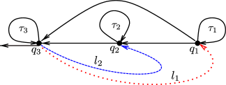
Figure 5: A pictorial representation of a production line, adapted from [1, §9.6.1], [20, §7.2]. The nodes $q_{1}$-$q_{3}$ denote machines and are associated with durations $\tau_{1}$-$\tau_{3}$ representing processing/recycling times. The two modes of operation can be distinguished by differently coloured arcs: i) Mode $l_{1}$ as red dotted line ($\cdots$), and ii) Mode $l_{2}$ with blue dashed line (- - -).

The network consists of nodes $q_{1}$, $q_{2}$, and $q_{3}$ where activities are performed with processing times $\tau_{1},\tau_{2},\tau_{3}\in\mathbb{N}$, respectively. The buffers between each pair of nodes have zero holding times and are all assumed to have a single product initially. The buffer before $q_{3}$ can store at most two incoming products. The other buffers are constrained to hold at most one product at a time. The node $q_{1}$ transfers product simultaneously to the buffers before $q_{2}$ and $q_{3}$. The earliest product arriving at $q_{3}$ is processed first.

The product exits node $q_{3}$ and then a new cycle is started. This is modelled as a feedback-loop from node $q_{3}$ to node $q_{1}$. In addition, we introduce a second mode of operation where the product from node $q_{3}$ is routed to node $q_{2}$ for reprocessing. This is distinguished by differently coloured arcs in Fig 5.

The state $x_{i}(k)\in\overline{\mathbb{R}}_{\varepsilon}$, for $i\in\{1,2,3\}$ and $k\in\mathbb{N}$, denotes the time when node $q_{i}$ finishes an activity for the $k$-th time. The convention is $x_{i}(k)=+\infty$ if no activity is performed at $q_{i}$ for the $k$-th time. It is assumed that all buffers contain a product initially. The dynamics of the production line can be expressed algebraically (as in (4)) as follows for mode $\ell(\cdot)=l_{1}$:

$$x_{1}(k+1) =\max\left(x_{1}(k)+\tau_{1},x_{2}(k),x_{3}(k)+\tau_{3}\right)$$ (25)

$$x_{2}(k+1) =\max\left(x_{1}(k)+\tau_{1},x_{2}(k)+\tau_{2}\right)$$

$$x_{3}(k+1) =\begin{aligned} \max(&x_{1}(k)+\tau_{1},x_{2}(k)+\tau_{2},x_{3}(k)+2\tau_{3},\\ &\min(x_{1}(k)+\tau_{1}+\tau_{3},x_{2}(k)+\tau_{2}+\tau_{3})).\end{aligned}$$

For the system dynamics in mode $\ell(\cdot)=l_{2}$, we have:

$$x_{1}(k+1) =\max\left(x_{1}(k)+\tau_{1},x_{2}(k)\right)$$ (26)

$$x_{2}(k+1) =\max\left(x_{1}(k)+\tau_{1},x_{2}(k)+\tau_{2},x_{3}(k)+\tau_{3}\right),$$

and the evolution of $x_{3}$ follows the same equation as of mode $l_{1}$. The initial state and output matrices ($y=C\otimes x$) are chosen as follows:

$$x(0) =\begin{pmatrix}0&0&\varepsilon\end{pmatrix}^{\top},\quad C=\begin{pmatrix}\varepsilon&\varepsilon&0\end{pmatrix}.$$ (27)

The dynamics can be represented in the min-max-plus conjunctive normal form (17), for $L=2$ and $M=1$, by replacing the expression of $x_{3}(\cdot)$ in (25) with

$$x_{3}(k+1)=\begin{aligned} \min\{&\begin{aligned} \max(x_{1}(k)+\tau_{1}+\tau_{3},x_{2}&(k)+\tau_{2},\\ &x_{3}(k)+2\tau_{3}),\end{aligned}\\ &\begin{aligned} \max(x_{1}(k)+\tau_{1},x_{2}(k)+&\tau_{2}+\tau_{3},\\ &x_{3}(k)+2\tau_{3})\}.\end{aligned}\end{aligned}$$ (28)

There are no continuous-valued inputs to the system. The discrete input $w(\cdot)\in\mathbb{V}\triangleq\{l_{1},l_{2}\}$ determines the mode as follows (see (4)):

$$\phi(\cdot,x,w)=\bigg{\{}i\in\{1,2\}\;\biggl{|}\;\min_{j\in\underline{L}}A^{(i,j)}\otimes x\in\overline{\mathbb{R}}^{n}_{\varepsilon}\setminus \{\varepsilon,\top\}^{n},$$ (29)

$$w=l_{i}\bigg{\}}.$$

The discrete-event system of the production network under consideration can therefore be expressed as a max-algebraic hybrid automaton as depicted in Fig. 3 with continuous-valued dynamics of the form (17).

As the system dynamics (25)-(26) satisfy Assumption 2, a finite-state discrete abstraction of the max-algebraic hybrid automaton can be obtained using Proposition 4. The necessity of the restriction of the state space $\mathbb{X}$ is reflected in the definition of the switching function $\phi(\cdot)$ in (29). The resulting one-step state transition graphs of the two modes are depicted in Fig. 6. Moreover, the reset relation does not entail transitions in continuous-valued state. Then the language of the max-algebraic hybrid automaton model of the production network is contained in the language of the obtained finite automaton.

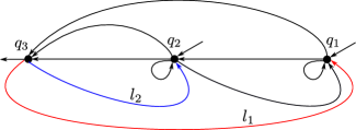
Figure 6: The one-step state transition graphs associated to the production network in Fig. 5. The finite automaton can be obtained by duplication of the nodes $q_{1}-q_{3}$ for the two modes $l_{1}$ and $l_{2}$. The black arcs are common to both the modes. The blue arc (—) belongs to mode $l_{2}$ and the red arcs (—) belong to mode $l_{1}$. The input and output arrows symbolise the initial and final states of the finite automaton.

This completes the illustration.

7 Conclusions

In this article, we have proposed a unifying max-algebraic hybrid automata framework for discrete-event systems in max-plus algebra. In this context, we identify the hybrid phenomena due to the interaction of continuous-valued max-plus dynamics and discrete-valued switching dynamics in switching max-plus linear and max-plus automata models. We have formally established the relationship between these two models and their relationships with the proposed max-algebraic hybrid automata framework utilising the notions of behavioural equivalence and bisimilarity. This is achieved in a behavioural framework where the models are seen as a collection of input-state-output trajectories. As a max-algebraic hybrid automaton and a max-plus automaton are defined on different state space, we have also studied their relationship by embedding them into their respective finite-state discrete abstractions.

In the future, we would like to identify the subclass of max-algebraic hybrid automata that can be simulated by a max-plus automaton. We would also like to address the relationships among timed Petri nets, extensions of max-plus automata and max-algebraic hybrid automata.

References

- [1] F. Baccelli, G. Cohen, G. J. Olsder, and J.-P. Quadrat. Synchronization and Linearity: An Algebra for Discrete Event Systems. John Wiley & Sons, 1992.
- [2] C. G. Cassandras and S. Lafortune. Introduction to Discrete Event Systems. Springer Science & Business Media, 2009.
- [3] G. Cohen, S. Gaubert, and J.-P. Quadrat. Algebraic system analysis of timed Petri nets. In Idempotency, pages 145–170. Cambridge University Press, 1997.
- [4] G. Cohen, S. Gaubert, and J.-P. Quadrat. Max-plus algebra and system theory: Where we are and where to go now. Annual Reviews in Control, 23:207–219, Jan. 1999.
- [5] B. De Schutter and T. J. van den Boom. Model predictive control for max-plus-linear discrete event systems. Automatica, 37(7):1049–1056, July 2001.
- [6] B. De Schutter and T. J. van den Boom. MPC for continuous piecewise-affine systems. Systems and Control Letters, 52(3-4):179–192, July 2004.
- [7] S. Gaubert. Performance evaluation of (max,+) automata. IEEE Transactions on Automatic Control, 40(12):2014–2025, 1995.
- [8] S. Gaubert and J. Mairesse. Modeling and analysis of timed Petri nets using heaps of pieces. IEEE Transactions on Automatic Control, 44(4):683–697, 1999.
- [9] J. Gunawardena. Min-max functions. Discrete Event Dynamic Systems: Theory and Applications, 4(4):377–407, 1994.
- [10] W. P. M. H. Heemels, B. De Schutter, and A. Bemporad. Equivalence of hybrid dynamical models. Automatica, 37(7):1085–1091, July 2001.
- [11] B. Heidergott, G. J. Olsder, and J. van der Woude. Max Plus at Work: Modeling and Analysis of Synchronized Systems: A Course on Max-Plus Algebra and its Applications. Princeton University Press, 2014.
- [12] A. A. Julius and A. J. van der Schaft. Bisimulation as congruence in the behavioral setting. In Proceedings of the 44th IEEE Conference on Decision and Control, pages 814–819, 2005.
- [13] J. Komenda, S. Lahaye, J. L. Boimond, and T. J. van den Boom. Max-plus algebra in the history of discrete event systems. Annual Reviews in Control, 45:240–249, Jan. 2018.
- [14] S. Lahaye, J.-L. Boimond, and J.-L. Ferrier. Just-in-time control of time-varying discrete event dynamic systems in (max,+) algebra. International Journal of Production Research, 46(19):5337–5348, 2008.
- [15] J. Lygeros, D. N. Godbole, and S. Sastry. Verified hybrid controllers for automated vehicles. IEEE Transactions on Automatic Control, 43(4):522–539, 1998.
- [16] J. Lygeros, G. Pappas, and S. Sastry. An introduction to hybrid system modeling, analysis, and control. In Preprints of the First Nonlinear Control Network Pedagogical School, pages 1–14, 1999.
- [17] J. Lygeros, C. Tomlin, and S. Sastry. Controllers for reachability specifications for hybrid systems. Automatica, 35(3):349–370, Mar. 1999.
- [18] C. A. Maia, L. Hardouin, R. Santos-Mendes, and B. Cottenceau. Optimal closed-loop control of timed event graphs in dioids. IEEE Transactions on Automatic Control, 48(12):2284–2287, Dec. 2003.
- [19] G. J. Olsder. Eigenvalues of dynamic max-min systems. Discrete Event Dynamic Systems: Theory and Applications, 1(2):177–207, Sept. 1991.
- [20] G. Soto Y Koelemeijer. On the Behaviour of Classes of Min-Max-Plus Systems. PhD thesis, Delft University of Technology, 2003.
- [21] F. D. Torrisi and A. Bemporad. HYSDEL - A tool for generating computational hybrid models for analysis and synthesis problems. IEEE Transactions on Control Systems Technology, 12(2):235–249, Mar. 2004.
- [22] T. J. van den Boom and B. De Schutter. Properties of MPC for max-plus-linear systems. European Journal of Control, 8(5):453–462, Jan. 2002.
- [23] T. J. van den Boom and B. De Schutter. Modelling and control of discrete event systems using switching max-plus-linear systems. Control Engineering Practice, 14(10):1199–1211, Oct. 2006.
- [24] T. J. van den Boom and B. De Schutter. Modeling and control of switching max-plus-linear systems with random and deterministic switching. Discrete Event Dynamic Systems: Theory and Applications, 22(3):293–332, Sept. 2012.
- [25] T. J. van den Boom, M. van den Muijsenberg, and B. De Schutter. Model predictive scheduling of semi-cyclic discrete-event systems using switching max-plus linear models and dynamic graphs. Discrete Event Dynamic Systems, 30(4):1–35, 2020.
- [26] A. J. van der Schaft. Equivalence of dynamical systems by bisimulation. IEEE Transactions on Automatic Control, 49d(12):2160–2172, Dec. 2004.
- [27] J. C. Willems and J. W. Polderman. Introduction to Mathematical Systems Theory: A Behavioral Approach. Springer-Verlag, New York, 1998.