Confinement and collective escape of active particles

Abstract

Active matter broadly covers the dynamics of self-propelled particles. While the onset of collective behavior in homogenous active systems is relatively well understood, the effect of inhomogeneities such as obstacles and traps lacks overall clarity. Here, we study how interacting self-propelled particles become trapped and released from a trap. We have found that captured particles aggregate into an orbiting condensate with a crystalline structure. As more particles are added, the trapped condensate escape as a whole. Our results shed light on the effects of confinement and quenched disorder in active matter.

Assemblies of interacting self-propelled particles, broadly defined as active matter, continue attracting significant attention Bechinger et al. (2016); Aranson (2013); Gompper et al. (2020). In the last ten years, notable progress was achieved in the understanding of the onset of collective behavior Chaté (2020); Peshkov et al. (2012); Patelli et al. (2019) and characterization of some collective states Solon et al. (2015); Alert et al. (2020). Spatial inhomogeneities, surface roughness, or quenched disorder play a significant role in active systems Peruani and Aranson (2018); Duan et al. (2021); Ro et al. (2021); Olsen et al. (2021). Quenched disorder, for example, may lead to the onset of trapped states, anomalous diffusion, and breakdown of ergodicity.

The motion of self-propelled particles on a disordered substrate is relevant in the context of the “active conductivity”. This situation is realized, for example, when motile bacteria propagate through a porous environment Waisbord et al. (2021). It is an analog of the equilibrium problem of electrons migration in random media. If the substrate is approximated as an array of well-separated traps (impurities), then the process can be viewed as a sequence of escapes and re-trappings of particles. In the context of electrons trapped by impurities, a non-zero conductance is due to the overlap of wave-functions of electrons at individual impurities (Dykhne theorem Bychkov and Dykhne (1971)). However, no such general result is known for active particles.

In this Letter, we study how self-propelled particles are captured and released by an isolated trap modeled as a potential well. We start with non-interacting particles and show that an individual particle typically exhibits chaotic scattering by a trap. Then we introduce interactions. A Lennard-Jones potential organizes particles into an orbiting condensate with the hexatic crystalline order. An alignment coupling brings dissipation and synchronization in the dynamics, and results in a perpetual capture of active particles: a trap becomes an analog of a “black hole”. “Bombardment” by active particles results in particle absorption, condensate melting, and recrystallization. Above a certain threshold number of captured particles, the trap storing capacity is exceeded, and the condensate escapes as a whole.

Active particles in a harmonic trap have been studied both experimentally Dauchot and Démery (2019); Schmidt et al. (2021); Takatori et al. (2016) and theoretically Pototsky and Stark (2012); Hennes et al. (2014); Wexler et al. (2020); Das et al. (2018); Jahanshahi et al. (2017). The main focus was on the steady-state distributions or escape of individual particles due to the combined effect of self-propulsion and thermal fluctuations. In this Letter, we consider purely deterministic effects of propulsion and interactions; this aspect of our model manifests a crucial difference not explored in other publications.

We consider a self-propelled particle moving in two dimensions with a constant velocity $V$, while a force $\mathbf{f}$ acting on the particle only rotates its direction of motion:

$$\frac{d{\bf r}}{dt}=\tilde{V}{\bf n}\;,\qquad\frac{d{\bf n}}{dt}=\mathbf{f}-({\bf n}\cdot\mathbf{f}){\bf n}\;.$$ (1)

Here ${\bf n}=(\cos\theta,\sin\theta)$ is the unit vector in the direction of motion. The equation for $\bf n$ ensures that $|{\bf n}|^{2}=1$. Thus, only the velocity direction changes and obeys $\dot{\theta}=f_{y}\cos\theta-f_{x}\sin\theta$. Physically, velocity aligns with the potential gradient. This situation can be realized, for example, for magnetic particles in a magnetic trap. Models of this type were also discussed in the context of artificial chemotaxis Liebchen et al. (2016); Liebchen and Löwen (2018); Stark (2018).

Below we consider different types of forces, but we start with a motion in an external potential field ${U}(x,y)$, so that $\mathbf{f}_{\rm pot}=-\nabla U$. If we renormalize variables so that the width and the depth of the potential are one, the only remaining relevant parameter is the dimensionless velocity $V$. The limit of strong potential is that of $V\to 0$. The corresponding equations can be written as

$$\frac{d{\bf r}}{dt} = V{\bf n}\;,$$ (2)

$$\frac{d\theta}{dt} = -\partial_{y}U\cos\theta+\partial_{x}U\sin\theta\;.$$ (3)

Equations (2), (3) possess the Hamiltonian

$$H({\bf r},{\bf p})=V|{\bf p}|-\exp\left[-\frac{U({\bf r})}{V}\right]=0\;.$$ (4)

Because of the energy conservation, the relation $|{\bf p}|=V^{-1}\exp[-U({\bf r})V^{-1}]$ holds. A substitution ${\bf p}=V^{-1}\exp[-U({\bf r})V^{-1}]{\bf n}$ reduces the Hamiltonian dynamics to Eqs. (2,3). The Hamiltonian (4) coincides with that describing ray propagation in geometrical optics, with the refraction index $\sim\exp[-U({\bf r})V^{-1}]$ Kravtsov and Orlov (1990).

In the small velocity limit, $V\ll 1$, one can separate slow migration of the particle (Eq. (2)) and its fast alignment with the gradient of the potential (Eq. (3)). The orientation angle $\theta$ in Eq. (3) adjusts to the gradient angle $\alpha=\arctan(\partial_{y}U/\partial_{x}U)$ as $\dot{\theta}=|\nabla U|\sin(\alpha-\theta)$. This fast adjustment of the direction of motion toward the minimum of the potential is followed by a slow drift (2). Once the vicinity of the potential minimum is reached, i.e., $|\nabla U|\approx 0$, the scale separation breaks down, and one has to consider the full Eqs. (2),(3).

In the vicinity of a minimum, a generic potential is approximated by an asymmetric parabolic well, $U_{\rm pb}=(x^{2}+b^{2}y^{2})/2$. Since the depth of this harmonic potential is not defined, one can set by virtue of a renormalization, parameter $V$ in Eqs. (2),(3) to one. Then the only parameter left is the potential asymmetry $b$. Since the dynamics is Hamiltonian, the type of motion depends on initial conditions.

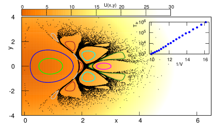
Figure 1: Poincaré map for a parabolic potential $b^{2}=\sqrt{5}-1$ (color background). Black dots: a chaotic trajectory starting at large $|x|,|y|$. The chaotic dynamics is not ergodic as it contains voids with closed curves - images of quasiperiodic trapped motion. Inset: Trapping time $T_{\rm tr}\sim\exp(1/V)$ in a Gaussian potential well vs velocity $V$, $b=(\sqrt{5}-1)/2$.

Figure 1 illustrates the dynamics for $b^{2}=\sqrt{5}-1$ (other values of $b$ give qualitatively the same picture). The three-dimensional phase space is reduced to a two-dimensional Poncaré map (we chose the section $\cos\theta=0$, $\frac{d}{dt}(\cos\theta)<0$). One sees a large chaotic domain (black dots) (video 1 in sup ) and regular islands filled with quasiperiodic trajectories. This Poincaré map is unusual for the Hamiltonian dynamics: the distribution is very inhomogeneous – density of points at small $\mathbf{r}$ values is much larger than at large ones. That happens because the “natural” coordinates $({\bf r},\theta)$ are not the canonical ones. One estimates the density on the plane $(x,y)$ by assuming a fully developed chaos where the angle $\theta$ is random and uniformly distributed. Then integration of a microcanonical distribution density for the Hamiltonian (4) $w({\bf r},{\bf p})\sim\delta\left(V|{\bf p}|-\exp\left[-\frac{U({\bf r})}{V}\right]\right)$ over the angle $\theta$ yields $W({\bf r})\sim\exp\left[-U({\bf r})/{V}\right]$. This resembles the Gibbs-Boltzmann distribution, with the velocity $V$ playing a role of the temperature. This result implies that the chaotic motion in Fig. 1 spreads to arbitrarily large values of the potential, although it is rather improbable to reach these heights. We conclude that although a slow particle arrives at the minimum of the potential and moves chaotically there, after a long time, it returns to the high values of the potential where it started. Such a return must happen according to the recurrence of the Hamiltonian trajectories. In addition to a chaotic region in Fig. 1, there are domains of quasi-periodic dynamics concentrated close to the potential minimum. This motion can occur for particles starting close to the minimum.

The Hamiltonian structure of Eqs. (2),(3) implies that capture of particles falling in a finite-depth potential well is impossible. Only temporary trapping occurs that can be interpreted as a chaotic scattering: a particle falls into the well, goes to its minimum, and moves there chaotically like in Fig. 1, but eventually rises high and escapes (video 2 in sup ). Furthermore, because of the exponential density $W\sim\exp[-U/V]$, the characteristic trapping time obeys a Kramers-like law $T_{\rm tr}\sim\exp[-1/V]$. This is confirmed in Fig. 1(inset) where the mean trapping time on a Gaussian potential well $U(x,y)=-\exp(-x^{2}-b^{2}y^{2})$ is shown.

We consider two types of interactions between particles below: (i) interaction by a potential force; (ii) an alignment to an average (over a neighborhood) orientation of neighboring particles; this latter interaction is of the Vicsek (or Kuramoto) type Vicsek et al. (1995); Chaté (2020).

Figure 2: Trajectories of three coupled particles in $(x,y)$ plane, for the LJ potential, for $V=0.1$ (a) and $V=0.2$ (b). Circles show positions of particles at time $t=100$, squares at time $t=500$. In panel (b) one sees the breakdown of the bounded state into a couple of particles moving to the left, and a particle moving to the right. (c) Average lifetime of a crystal of $N$ particles vs inverse velocity $1/V$. The dissociation time is defined as an event when one particle leaves.

We start with the interaction via a conservative pair-wise force that depends on the distance between the particles. This case, like the motion in the external potential above, is Hamiltonian. We explore below the Lennard-Jones (LJ) potential $U_{\rm LJ}({\bf r}_{1},{\bf r}_{2})=4(\rho^{-12}-\rho^{-6})$, where $\rho^{2}=|{\bf r}_{1}-{\bf r}_{2}|^{2}$. Several particles having a small velocity $V$ placed close to each other, form a bounded state due to the LJ-coupling. For two particles, the bounded state is quasiperiodic, while for $N\geq 3$ it is typically chaotic. Several particles form a chaotically vibrating “crystalline molecule” with a hexatic order. The center of mass (c.o.m.) performs a diffusive motion in the plane $(x,y)$, and the particles from time to time rearrange their positions, see Fig. 2(a,b) and Video 4 in sup . Because the LJ potential is finite, there is a non-zero probability for a particle to escape. Such an event is shown in Fig. 2(b). Figure 2(c) shows that the lifetime $T_{\rm LJ}$ of a “shaking crystal” without confining potential has the same Kramers-type dependence on the velocity $T_{\rm LJ}\propto\exp[V^{-1}]$, as the lifetime of a particle in a potential well (cf. Fig. 1(inset)). A crystalline molecule has a significant lifetime only for particles with $V\lesssim 0.5$.

The aligning force $\mathbf{F}_{k}$ acts in the direction of the weighted average of the velocities of other particles in a neighborhood of $k$-th particle:

$$\mathbf{F}_{k}=\epsilon\sum_{j}S(|\mathbf{r}_{j}-\mathbf{r}_{k}|)\mathbf{n}_{j}\;.$$ (5)

The distance-dependent factor (we assume it to be Gaussian $S(r)=\exp(-r^{2}/r_{0}^{2})$) defines the range $r_{0}$ of the force. Parameter $\epsilon$ determines the strengths of the alignment. The alignment force is velocity-dependent and dissipative. In terms of the velocity direction $\theta$ it has the form of Kuramoto-type coupling $\dot{\theta}_{k}\sim\sin(\theta_{j}-\theta_{k})$.

We examine next a combination of the alignment and the conservative forces due to a confining potential or an LJ interaction (for a pure alignment see Kruk et al. (2018)).

We start with a set of chaotic particles in a harmonic trap (Fig. 1), described by Eqs. (2),(3) with additional alignment (5). The main observation is that for large values of $\epsilon$ and large ranges of coupling $r_{0}$, particles always synchronize: after some transient time, all the coordinates and angles coincide, and the particles form a synchronous point cluster ${\bf r}_{1}=\ldots={\bf r}_{N}$, $\theta_{1}=\ldots=\theta_{N}$ (video 3 in sup ). This synchronization is possible because the aligning force is dissipative Peruani and Aranson (2018). In the final synchronous state dissipation disappears (the force $\sim\sin(\theta_{j}-\theta_{k})$ vanishes), and the trajectory of the cluster is described again by the Hamiltonian dynamics (2),(3). However, in the course of alignment, particles leave the chaotic domain, and the final dynamics is quasiperiodic (cf. Fig. 1). Thus, strong alignment synchronizes particles and regularizes their motion. For lower alignment rates $\epsilon$ and especially for small ranges $r_{0}$, multiple states with several clusters are observed up to large times. If the alignment coupling radius $r_{0}$ is small enough, several regular clusters may effectively stop to interact; then they constitute an “attractor”. Noteworthy, standard methods of the synchronization theory, like the master stability function method Pecora and Carroll (1998), are not applicable here because the type of motion (from chaos to quasiperiodicity) changes over time. In Fig. 3(a) we illustrate the rate of synchronization in dependence on the parameters $\epsilon$ and $r_{0}$. At large $r_{0}$ there is an “optimal” coupling strength. We attribute this to the fact that, for large $r_{0}$, the alignment coupling is a global one. Because the velocities of distant particles are effectively “de-aligned” by different potential forces they experience at different positions in the harmonic trap, the alignment slows down. At small values of $r_{0}$, only neighboring particles interact, and they are much more “synchronizable” because their trajectories in the potential may easily adjust as well.

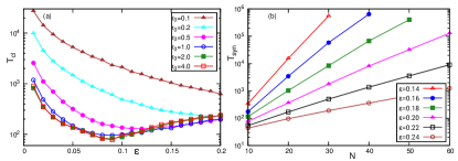
Figure 3: (a) The average time at which 20 initially randomly distributed particles in a harmonic potential form 10 clusters due to alignment. For small $r_{0}$ this time monotonously decreases with coupling strength $\epsilon$, while large ranges of $r_{0}\gtrsim 0.5$ there is an optimal coupling strength. (b) Average time to synchronization for chaotic crystals composed of $N$ particles, for $V=0.1$ and different strengths of alignment forces $\epsilon$.

In the case of alignment of particles trapped by a finite-depth potential well, two time scales compete: the trapping time $T_{\rm tr}$ determined by the velocity $V$ (cf. Fig. 1(inset)); the synchronization time $T_{\rm s}$ (e.g., one can take the clustering time of Fig. 3(a)). If $T_{\rm s}\gg T_{\rm tr}$, almost all the particles escape from the well and spread. In the opposite limit, $T_{\rm s}\ll T_{\rm e}$, a complete self-trapping due to alignment occurs: a cluster of synchronous trapped quasiperiodically moving particles appears. Thus, the potential well becomes an effective “black hole”: particles are trapped perpetually due to dissipative alignment. In an intermediate case $T_{\rm s}\sim T_{\rm tr}$, some particles escape while others form a perpetually trapped cluster.

A combination of the LJ and the alignment interactions allows for synchronization of the crystal. Point clusters cannot be formed because particles cannot come close to each other due to the LJ repulsion at small distances. Thus, only orientations $\theta_{k}$ can synchronize. Here again, a relation between the synchronization time and the lifetime due to potential forces is crucial.

We describe the combined action of the LJ and alignment interactions for particles in the finite-well potential, because, for small enough velocities, the particles are practically trapped forever. We chose the width of the well to be approximately ten times larger than the characteristic spatial scale of the LJ potential so that only a few particles fit into the well.

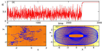
Figure 4: Seven particles with a LJ potential and alignment in a potential well (color coding). Panel (a): the order parameter $R$ vs time. Panels (b,c): trajectories of the c.o.m on the $(x,y)$ plane in the disordered $t<2300$ (b) and in the ordered $t>3000$ (c) domains.

Figure 4 illustrates the dynamics of seven particles. Initially, they form a shaking crystal with a random motion (reminiscent of a confined random walk) of the c.o.m, Fig. 4(b). The orientational order is characterized by the Kuramoto order parameter $R=|\langle e^{i\theta}\rangle|$, Fig. 4(a). In the disordered state, the order parameter fluctuates around $R\approx 0.4$. At $t\approx 2500$, an abrupt transition to synchrony in the directions of motion is observed, beyond this transition $R\approx 1$. The crystal becomes ordered, and the c.o.m. performs a quasiperiodic motion in the well, Fig.  4(c), and all the particles become perpetually trapped (video 5 in sup ).

The abrupt transition to synchrony from a chaotic crystal should be contrasted to the clustering transition without the LJ coupling. In the latter case, the order parameter grows gradually as the particles continuously come closer and merge. In contradistinction, the process depicted in Fig.  4(a) is characterized as transient chaos that abruptly ends in an absorbing synchronized state (see a general exposition of transient chaos Lai and Tél (2011), and a case of chiral active particles in Pikovsky (2021)).

To examine the dependence of the synchronization time on the size of the crystal, we consider a set of $N$ active particles. We take the LJ interaction and additional alignment coupling with $r_{0}=1$ (i.e., the same range as the LJ potential) but without a confining external potential. To ensure that the lifetime of the crystal is larger than a characteristic synchronization time (cf. Fig. 2(c)), we considered particles with small velocity $V=0.1$. Figure 3(b) shows that the dependence of the synchronization time on the size of the crystal is exponential $T_{\rm syn}\sim g(\epsilon)\exp[h(\epsilon)N]$, with $\epsilon$-dependent factors $g,h$. That implies that here a super transient behavior Lai and Tél (2011); Pikovsky (2021) is observed, for which a characteristic time exponentially grows with the system size.

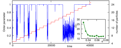
Figure 5: An example of trapping dynamics for $\epsilon=0.04$ and $V=0.15$ (a particle is added every 2000 time units). Blue line: evolution of the order parameter (left axis) showing domains of disorder and synchrony ($R\approx 1$). Red curve: number of particles (right axis). Inset: the average size of the escaped cluster vs $\epsilon$. The time interval is proportional to the size of the cluster because a particle is added every 2000 time units.

Finally, we studied how many particles can be trapped in a potential well in the process illustrated in Fig. 4. We assume for simplicity that $r_{0}=\infty$, i.e., all particles in the well equally contribute to the alignment. The particles from outside “bombard” the trap one-by-one at regular time intervals. They form a crystal, the dynamics of which is followed using the alignment order parameter $R$, see Fig. 5. One sees that in some cases adding a particle melts the crystal. In other cases, a particle is absorbed into the existing order. Finally, the crystal as a whole escapes the potential well because an incoming particle “kicks” it from a trapped quasiperiodic regime into an escaping trajectory. We observed that only a synchronized crystal can escape (video 6 in sup ). Fig. 5(inset) depicts the average size of the escaping crystal $\langle S\rangle$ vs $\epsilon$. It shows a significant increase of a typical escaping crystal size for low alignment rates $\epsilon$. That occurs because for global coupling, the alignment rate is proportional to the number of particles. Therefore, for small $\epsilon$, a sufficient number of interacting particles is required to form a synchronous crystal.

In conclusion, we investigated the trapping of individual and interacting active particles. The problem is nontrivial for slow particles (deep potentials), that spend a long time close to the bottom. We have found that non-interacting particles can be trapped only for a finite time due to the Hamiltonian structure of the equations of motion. In turn, an alignment of particles brings dissipation and establishes a time arrow. So, the potential well becomes a “black hole” with perpetually captured particles on quasiperiodic trajectories. The particles form either a cluster or a coherent crystal if additional LJ coupling is taken into account. With the particle bombardment, we observe a highly nontrivial trapping behavior: melting and re-synchronization of crystals, and eventually a coherent escape of the entire assembly.

The problem we have studied is relevant for the understanding of active matter subject to quenched environmental disorder. For the media, which can be interpreted as an array of randomly positioned traps, the process can be represented as a sequence of the described above trapping events. Our study also shows that the disorder may have a finite trapping capacity. Once the traps are filled up, the further bombardment may lead to the spontaneous avalanche-like release of many particles. While this phenomenon is reminiscent of self-organized criticality (SOC) Bak et al. (1988), there are many fundamental differences: the trapped states are highly dynamic and form chaotically or coherently moving crystals. Likely, this will result in a different distribution for the avalanche sizes and other statistical characteristics.