Impact of spatial coarsening on Parareal convergence

Abstract

We study the impact of spatial coarsening on the convergence of the Parareal algorithm, both theoretically and numerically. For initial value problems with a normal system matrix, we prove a lower bound for the Euclidean norm of the iteration matrix. When there is no physical or numerical diffusion, an immediate consequence is that the norm of the iteration matrix cannot be smaller than unoty as soon as the coarse problem has fewer degrees-of-freedom than the fine. This prevents a theoretical guarantee for monotonic convergence, which is necessary to obtain meaningful speedups. For diffusive problems, in the worst-case where the iteration error contracts only as fast as the powers of the iteration matrix norm, making Parareal as accurate as the fine method will take about as many iterations as there are processors, making meaningful speedup impossible. Numerical examples with a non-normal system matrix show that for diffusive problems good speedup is possible, but that for non-diffusive problems the negative impact of spatial coarsening on convergence is big.

68Q25, 68R10, 68U05

1 Introduction

To unlock the performance of future high-performance computing systems with their rapidly increasing number of compute cores, parallelisable numerical algorithms are needed. For the solution of time-dependent partial differential equations (PDEs), parallel-in-time methods are considered a promising way to provide more concurrency [3]. The most widely studied algorithm of this type is Parareal [24]. Other popular “parallel-across-the-steps” methods in the terminology of Gear [14] are MGRIT [7] or PFASST [6]. Surveys of the field have been provided by Gander [11] and Ong and Schroder [26].

These “parallel-across-the-steps” methods solve initial value problems in a way that allows to compute the solution on multiple time steps in parallel. To achieve this, they use a hierarchy of levels, similar to multi-grid methods, where the unavoidable serial dependency in time is shifted to the coarsest, computationally cheapest level. While this still leaves a serial bottleneck, it frees up the computationally costly computations on the fine levels for concurrency. Multiple studies have shown that parallel-in-time integration in combination with spatial parallelism can provide more speedup than parallelising in space alone [7, 25, 31].

The key to good performance in these methods is to build a computationally cheap coarse level to minimise the serial bottleneck without compromising rapid convergence. When solving PDEs, an attractive option is to coarsen the resolution of the spatial discretisation: in three dimensions, coarsening spatial resolution by half will reduce cost by a factor of $2^{3}=8$ in contrast to coarsening in time which will only deliver a factor of two. For Parareal, this strategy seems to have first been studied by Fischer et al. [8]. They use a finite element based discretisation of the Navier-Stokes equations and find that Parareal can converge reasonably fast if $l_{2}$-projection is used to transfer between coarse and fine mesh. Simple interpolation is found to cause stability issues. Later, a short numerical investigation of spatial coarsening for Parareal showed that interpolation for simple problems can work but that performance depends on spatial resolution and the used interpolation order [27]. Some theory for Parareal with spatial coarsening for the linear advection equation in one dimension with an upwind discretisation is developed by Gander [10]. A detailed analysis of convergence bounds for both Parareal and MGRIT is provided by Southworth [30]. While their approach allows to consider spatial coarsening, its effect is not analysed in detail. Howse at al. present a heuristic adaptive strategy for spatial coarsening in MGRIT and demonstrate in numerical examples that their approach can resolve shock formation in Burgers’ equation [22]. An investigation into the impact of spatial coarsening on MGRIT performance is in progress but has not yet been published [29].

Besides these papers, there seems to have been little systematic analysis of what the impact of spatial coarsening on convergence of Parareal is. There is a number of papers that analyse Parareal based on Dahlquist’s test equation or variants thereof [12, 13, 28, 2]. While the test equation can produce reliable results for general linear value problems by means of diagonalisation, spatial coarsening means that dimensions of the the coarse and fine level problems are different and it is unclear how to apply the approach in this case.

This paper will investigate the impact of spatial coarsening on the convergence of Parareal both theoretically via the norm of the error propagation and by numerical experiments. For linear initial value problems with a normal system matrix, we prove a lower bound for the error propagation matrix $l_{2}$-norm when coarsening is used. The bound is independent of the specifics of the coarse propagator and only depends on the fine propagator, the number of degrees-of-freedom on the coarse mesh and the eigenvalues of the system matrix. We discuss implications of this results and show numerical examples that illustrate the impact of spatial coarsening on Parareal convergence for problems with both normal and non-normal system matrices. Although the norm of the iteration matrix provides only an upper bound for convergence, showing that is is smaller than unity would give a theoretical guarantee for monotonic convergence. This would rule out the error growth often observed in particular for hyperbolic problems [12], which makes obtaining speedup nearly impossible. Our result suggests that in particular for non-diffusive problems, finding such a bound will be very challenging when any form of spatial coarsening is used and that other theoretical tools may be needed.

2 Parareal with spatial coarsening for linear problems

Consider a linear initial value problem

(1) $$\partial_{t}y(t)=Ay(t),\ y(0)=b,\ t\in[0,T],$$

with $A\in\mathbb{C}^{n\times n}$, $b\in\mathbb{C}^{n}$. We will typically think of (1) as arising from the semi-discretisation of a partial differential equation, but this need not be the case. We decompose the time interval $[0,T]$ into $P$ so-called time-slices so that

(2) $$[0,T]=[0,t_{1}]\cup[t_{2},t_{3}]\cup\ldots[t_{P-1},t_{P}]$$

with $t_{P}=T$. Let $\mathcal{F}_{\delta t}$ and $\mathcal{G}_{\Delta t}$ be one-step numerical timestepping methods. Parareal computes an approximate solution to (1) via the iteration

(3) $$y^{k+1}_{j+1}=\mathcal{G}_{\Delta t}(y^{k+1}_{j})+\mathcal{F}_{\delta t}(y^{k}_{j})-\mathcal{G}(y^{k}_{j})$$

for $j=0,\ldots,P-1$. As the iteration converges, it will reproduce the solution

(4) $$y_{j+1}=\mathcal{F}_{\delta t}(y_{j})$$

provided by running $\mathcal{F}_{\delta t}$ in the typical step-by-step fashion.

Note that since the values $y^{k}_{j}$ are known from the previous iteration, the computation of $\mathcal{F}_{\delta t}(y^{k}_{j})$ in (3) can be parallelised across $P$ processing units. By contrast, $\mathcal{G}_{\Delta t}(y^{k+1}_{j})$ must be computed serially step-by-step. Therefore, $\mathcal{F}_{\delta t}$ should be accurate but can be computationally expensive and is thus called the fine propagator. By contrast, since $\mathcal{G}_{\Delta t}$ runs serially, it must be computationally cheap but can be inaccurate and is thus called the coarse propagator.

Spatial coarsening

An effective way to reduce computational cost of the coarse method is to use a coarser spatial discretisation. In that case, a differential equation

(5) $$\partial_{t}\tilde{y}(t)=\tilde{A}\tilde{y}(t)$$

with $\tilde{A}\in\mathbb{C}^{m\times m}$, $\tilde{y}(t)\in\mathbb{C}^{m}$ and $m<n$ is solved numerically on the coarse level. A restriction operator $R\in\mathbb{C}^{m\times n}$ transfers the solution from the fine to the coarse level and an interpolation operator $I\in\mathbb{C}^{n\times m}$ from the coarse to the fine [8]. One application of the coarse method in Parareal then becomes

(6) $$\mathcal{G}_{\Delta t}=I\tilde{\mathcal{G}}_{\Delta t}(Ry)$$

where $\tilde{\mathcal{G}}_{\Delta t}$ is the coarse method applied to (5).

2.1 Parareal for linear problems as a stationary iteration

For the linear problem (1) and one-step methods as propagators we can write

(7) $$\mathcal{F}_{\delta t}(y)=R_{f}(\delta tA)^{N_{f}}y=:Fy$$

and

(8) $$\mathcal{G}_{\Delta t}(y)=IR_{g}(\Delta t\tilde{A})^{N_{g}}Ry=:I\tilde{G}Ry=:Gy,$$

where $R_{f}(z)$ and $R_{g}(z)$ are the stability functions, and $N_{f},N_{g}$ are the number of time steps per time slice for fine and coarse propagator, respectively. That is, the action of both propagators can be expressed as multiplication with matrices $F\in\mathbb{C}^{n\times n}$ and $G\in\mathbb{C}^{n\times n}$. In this case, it is straightforward to interpret Parareal as a stationary fixed point iteration [1]. Application of the fine propagator directly via (4) can be written as

(9) $$\mathbf{M}_{f}\mathbf{y}_{f}:=\begin{pmatrix}1\\ -F&1\\ &\ddots&\ddots\\ &&-F&1\end{pmatrix}\begin{pmatrix}y_{0}\\ y_{1}\\ \vdots\\ y_{P}\end{pmatrix}=\begin{pmatrix}b\\ 0\\ \vdots\\ 0\end{pmatrix}$$

where $1$, in a slight abuse of notation, denotes the $n\times n$ identity matrix. The Parareal iteration (3) reads

(10) $$y^{k+1}_{j+1}=Gy^{k+1}_{j}+Fy^{k}_{j}-Gy^{k}_{j}$$

for $j=0,\ldots,P-1$ with $y^{k}_{0}=0$ and can be written

(11) $$\mathbf{M}_{g}\mathbf{y}^{k+1}=\left(\mathbf{M}_{g}-\mathbf{M}_{f}\right)\mathbf{y}^{k}+\mathbf{b}$$

with $\mathbf{M}_{g}$ defined analogously to $\mathbf{M}_{f}$ in (9) and

(12) $$\mathbf{b}=\begin{pmatrix}b\\ 0\\ \vdots\\ 0\end{pmatrix}.$$

Let $\mathbf{y}_{f}$ be the serial fine solution of (9). Then, the iteration error $\mathbf{e}^{k}:=\mathbf{y}_{f}-\mathbf{y}^{k}$ is given by

(13) $$\mathbf{e}^{k}=\mathbf{E}\mathbf{e}^{k-1}=\mathbf{E}^{k}\mathbf{e}_{0}$$

with $\mathbf{E}=\mathbf{M}_{g}^{-1}\left(\mathbf{M}_{g}-\mathbf{M}_{f}\right)$.

Lemma 2.1.

The error propagation matrix is given by

(14) $$\mathbf{E}=\begin{pmatrix}0&\\ B_{0}&0\\ B_{1}&B_{0}&0\\ &\ddots&\ddots&\ddots\\ B_{P-1}&\ldots&B_{1}&B_{0}&0\end{pmatrix}$$

with

(15) $$B_{k}=G^{k}\left(F-G\right).$$

Proof 2.2.

First, it is easy to confirm that

(16) $$\mathbf{M}_{g}^{-1}=\begin{pmatrix}1\\ G&1\\ G^{2}&G&1\\ \vdots&&\ddots&\ddots\\ G^{P-1}&\ldots&G^{2}&G&1\end{pmatrix}.$$

Then, some matrix algebra shows that

(17) $$\mathbf{E}=\begin{pmatrix}1\\ G&1\\ G^{2}&G&1\\ \vdots&&\ddots&\ddots\\ G^{P-1}&\ldots&G^{2}&G&1\end{pmatrix}\begin{pmatrix}0&\\ F-G&0\\ &F-G&0\\ &&\ddots&\ddots\\ &&&F-G&0\end{pmatrix}$$

has the form shown above.

2.2 Increment and error

Since the error requires knowledge of the fine solution which is normally not available, a commonly used approach is to monitor converge of Parareal via the difference between two iterates

(18) $$\Delta^{k}_{j}:=y^{k+1}_{j}-y^{k}_{j}$$

for $j=1,\ldots,P$. Although the connection between defect and iteration error shown below is straightforward, it does not appear to have been documented in the literature so far and the issue of how good a predictor the defect is for the error seems to not have been considered at all.

Lemma 2.3.

For the Parareal iteration (3) applied to a linear problem (1) where both propagators are one-step methods, the increment between two iterations

(19) $$\mathbf{\Delta}^{k}=\mathbf{y}^{k+1}-\mathbf{y}^{k}.$$

is given by

(20) $$\mathbf{\Delta}^{k}=\mathbf{e}^{k+1}-\mathbf{e}^{k}=\mathbf{E}^{k}\left(\mathbf{E}-1\right)\mathbf{e}_{0}.$$

Proof 2.4.

Using (13) we have

(21) $$\mathbf{\Delta}^{k}=\mathbf{y}^{k+1}-\mathbf{y}_{f}+\mathbf{y}^{f}-\mathbf{y}^{k}=\mathbf{e}^{k+1}-\mathbf{e}^{k}=\mathbf{E}^{k}\left(\mathbf{E}-1\right)\mathbf{e}_{0}.$$

This implies that if $\left\|\mathbf{E}\right\|<1$ the defect and error contract at the same rate since

(22) $$\left\|\mathbf{\Delta}^{k}\right\|\leq C\left\|\mathbf{E}\right\|^{k}$$

and

(23) $$\left\|\mathbf{e}^{k}\right\|\leq\tilde{C}\left\|\mathbf{E}\right\|^{k}$$

for some constants $C$, $\tilde{C}$. However, it also means that if the error for some time slice does not change in an iteration, the corresponding defect will be zero. This raises the possibility that there might be scenarios where checking the defect for convergence will give a “false positive” result where the defect is small and the iteration stops although the error is actually large. Investigating this is left for future work.

2.3 Norm of $\mathbf{e}^{k}$ versus norm of $\mathbf{E}^{k}$ versus $\left\|\mathbf{E}\right\|_{2}^{k}$

From (13), we can bound the Parareal error as

(24) $$\left\|\mathbf{e}^{k}\right\|_{2}=\left\|\mathbf{E}^{k}\mathbf{e}^{0}\right\|_{2}\leq\left\|\mathbf{E}^{k}\right\|_{2}\left\|\mathbf{e}^{0}\right\|_{2}\leq\left\|\mathbf{E}\right\|_{2}^{k}\left\|\mathbf{e}^{0}\right\|_{2}.$$

Remember that $\mathbf{E}$ is nil-potent. Therefore, its spectral radius is zero and the error always goes to zero asymptotically. However, for Parareal to provide speedup, we need the error to contract fast and in particular we want it to decrease monotonically.

This can be guaranteed theoretically if $\left\|\mathbf{E}\right\|_{2}<1$. However, even if $\left\|\mathbf{E}\right\|_{2}>1$, it is possible for the norm of $\mathbf{E}^{k}$ to decrease monotonically, also leading to error contraction although whether this happens or not will depend on the specific setup. Interestingly, the results below show that depending on the initial value, we can also have scenarios where $\left\|\mathbf{E}^{k}\right\|_{2}$ grows but $\left\|\mathbf{e}^{k}\right\|_{2}$ decays.

2.4 Numerical and physical diffusion

We assume that no eigenvalue of $A$ in (1) has positive real part, otherwise the problem is not well-posed. If the initial value problem (1) is advanced in time exactly, we get

(25) $$y(t_{j+1})=\exp(A\delta t)y(t_{j}).$$

Eigenvalues with negative real part give rise to exponentially decaying solutions. If this is a property of the problem like in the heat equation, we call this effect physical diffusion. If the original problem is non-diffusive and the negative real parts come from the employed spatial discretisation, we refer to this as spatial numerical diffusion. Here, diffusion is purely an artifact of the numerics and will vanish as the spatial resolution is refined. An example would be an upwind finite difference discretisation of the linear advection equation $u_{t}+u_{x}=0$ with periodic boundary conditions [4, Eq. (3.35)], see Figure 1 (left). The PDE is non-diffusive but the eigenvalues of $A$ have negative real-part. Consequently, the eigenvalues of $\exp(A\delta t)$ lie inside the unit circle, which will result in amplitudes going to zero as $t\to\infty$. By contrast, the non-diffusive centered finite difference approximation [4, (Eq. (3.28)] means that all eigenvalues of $A$ lie on the imaginary axis and thus the eigenvalues of $\exp(A\delta t)$ are on the unit circle so that amplitudes are preserved, see Figure 1 (right).

Numerical diffusion can also be introduced by the time stepping scheme. The fully discrete solution does not evolve according to (25) but

(26) $$y_{j+1}=R(A\delta t)y_{j},$$

where $R$ is the stability function of the used one-step method and $y_{j}\approx y(t_{j})$ is the resulting numerical approximation. Even when there is no physical or spatial numerical diffusion and all eigenvalues of $A$ have real part equal to zero, $R(A\delta t)$ might have eigenvalues with negative real part. In that case, the numerical solution will also decay exponentially as $t\to 0$. We call this temporal numerical diffusion and it will vanish in the limit $\delta t\to 0$. Trefethen discusses these effects in more detail [32].

Figure 1: Eigenvalues of $A$ for a first order upwind (left) or second order centered (right) finite difference discretisation of the linear advection equation.

3 Lower bound for the Parareal iteration matrix norm

The main theoretical result of this paper is the following theorem. Its implications are discussed in Subsection 3.1 and the proof is given in Subsection 3.2.

Theorem 3.1.

Consider a linear initial value problem (1) with a normal matrix $A$ with eigenvalues $\lambda_{1},\ldots,\lambda_{n}$ ordered by decreasing absolute value, that is $|\lambda_{1}|\geq|\lambda_{2}|\geq\ldots|\lambda_{n}|$. Let $\mathcal{F}_{\delta t}$ and $\mathcal{G}_{\Delta t}$ be one-step methods with rational stability functions $R_{f}(z)$ and $R_{g}(z)$ and let the fine method be stable, so that $\left|R_{f}(\lambda_{j}\delta t)\right|\leq 1$ for $j=1,\ldots,n$. Assume that the coarse propagator $\mathcal{G}_{\Delta t}$ is solving a coarsened linear initial value problem (5) with dimension $m<n$ and that interpolation and restriction operators $I\in\mathbb{C}^{n\times m}$ and $R\in\mathbb{C}^{m\times n}$ are used. Then, the $l_{2}$-norm of Parareal’s error propagation matrix is bounded from below by

(27) $$\left\|\mathbf{E}\right\|_{2}\geq\sqrt{\sum_{j=m+1}^{n}\left|R_{f}(\lambda_{j}\delta t)^{N_{f}}\right|^{2}}\geq\left|R_{f}(\lambda_{m+1}\delta t)^{N_{f}}\right|.$$

Remark 3.2.

The bound in Theorem 3.1 is independent of the choice of coarse method, coarse time step or interpolation or restriction operator, that is, independent of $R_{g}$, $\Delta t$, $I$ and $R$.

Remark 3.3.

Standard finite difference discretisation on equidistant meshes with periodic boundary conditions, for example, give rise to a matrix $A$ that is circulant and thus normal. Furthermore, symmetric/Hermitian and skew-symmetric/skew-Hermitian matrices are normal. For a comprehensive characterisation of normal matrices see e.g. the book by Horn and Johnson [21, Sec. 2.5] and the paper by Grone et al. [17].

3.1 Implications of Theorem 3.1

The matrix $\mathbf{E}$ is nil-potent with $\mathbf{E}^{P}=0$, reflecting the well-known fact that Parareal always converges when the number of iterations is equal to the number of time slices. Therefore, even if the norm of the error matrix is large, Parareal will still converge for any initial guess. This is, however, not enough to make it useful: since $\mathbf{M}_{f}$ has a lower diagonal block-structure, problem (9) can easily be solved by forward substitution, which corresponds to running the fine method in serial. Speedup from Parareal after $K$ iterations on $P$ time slices/processors is bounded by

(28) $$S(P)\leq\min\left\{\frac{P}{K},\frac{\text{Runtime of }\mathcal{F}_{\delta t}}{\text{Runtime of }\mathcal{G}_{\Delta t}}\right\}.$$

Spatial coarsening can significantly reduce the computational cost of the coarse propagator and thus improve the second bound. However, it increase the number of iterations required for convergence and reduce the first bound. For Parareal to deliver speedup, it needs to converge in a number of iterations that is much smaller than the number of time slices or $K\ll P$. This can be guaranteed theoretically if

(29) $$\left\|\mathbf{E}\right\|\ll 1$$

in a suitable norm, see also the discussion by Buvoli and Minion [2]. Therefore, a result that proofs that $\left\|\mathbf{E}\right\|<1$ holds under certain conditions would be very desirable. Theorem 3.1 shows that if spatial coarsening is used, such a guarantee will be difficult to find for non-diffusive problems. Note, however, that $\left\|\mathbf{E}\right\|<1$ is only a sufficient condition for the iteration to converge, not a necessary one [23, Corollary 1.2.1]. This means that we may see the iteration converge despite the norm being larger than one. Our numerical examples in Section 4.1 show that actual convergence is often monotonic, even when the norm of $\mathbf{E}$ is larger than one and would permit non-monotonic convergence. However, we also see that convergence is typically very slow in these cases and that the impact of spatial coarsening on convergence speed can be substantial.

Remark 3.4.

We can make Parareal converge arbitrarily fast by changing the norm. Since the spectral radius of $\mathbf{E}$ is zero, for any $\varepsilon>0$ there exists a norm on $\mathbb{C}^{n}$ with

(30) $$\left\|\mathbf{E}\right\|\leq\varepsilon$$

in the associated matrix norm [23, Theorem 1.3.1]. But having to cherry-pick the norm and thus the way to measure errors only to make Parareal converge is hardly a satisfactory solution.

Corollary 3.5.

For a fine method of order $p$ we have

(31) $$\left\|\mathbf{E}\right\|_{2}\geq\left|\exp(\lambda_{m+1}\Delta t)\right|+\mathcal{O}(\delta t^{p+1})$$

as $\delta t\to 0$.

Proof 3.6.

It holds that

(32) $$R_{f}(z)=\exp(z)+\mathcal{O}(|z|^{p+1})\ \text{as}\ |z|\to 0$$

where $p$ is its order of consistency [18, p. 42]. Therefore, with $z=\lambda_{m+1}\delta t$ and $\Delta t=\delta tN_{f}$,

(33a) $$\left\|\mathbf{E}\right\|_{2} \geq\left|R_{f}(\lambda_{m+1}\delta t)\right|^{N_{f}}$$

(33b) $$=\left|\exp(\lambda_{m+1}\delta t)+\mathcal{O}(|\lambda_{m+1}\delta t|^{p+1})\right|^{N_{f}}$$

(33c) $$=\left|\exp(\lambda_{m+1}\delta t)^{N_{f}}\right|+\mathcal{O}(|\lambda_{m+1}|^{p+1}\delta t^{p+1})$$

(33d) $$=\left|\exp(\lambda_{m+1}\Delta t)\right|+\mathcal{O}(\delta t^{p+1}).$$

Remark 3.7.

For problems without physical or spatial numerical diffusion, this means that using spatial coarsening eliminates any chance for a theoretical guarantee for good convergence: if all $\lambda_{n}$ are purely imaginary, Corollary 3.5 implies

(34) $$\left\|\mathbf{E}\right\|_{2}=1+\mathcal{O}(\delta t^{p+1})$$

as $\delta t\to 0$.

Remark 3.8.

When there is physical or spatial numerical diffusion present, the case is less clear. If $\text{Re}(\lambda_{m+1})\Delta t\ll 0$, bound (27) allows $\left\|\mathbf{E}\right\|_{2}\ll 1$. However, with $A=U\Sigma U^{*}$, note that the exact solution of (1) is

(35) $$y_{\text{exact}}=U\exp(\Sigma T)U^{*}y_{0},$$

so that

(36a) $$\left\|y_{\text{exact}}\right\|^{2}_{2} =\sum_{j=1}^{n}\left(\exp(\lambda_{j}T)y_{0}^{(j)}\right)^{2}$$

(36b) $$=\sum_{j=1}^{m}\left(\exp(\lambda_{j}T)y_{0}^{(j)}\right)^{2}+\sum_{j=m+1}^{n}\left(\exp(\lambda_{j}T)y_{0}^{(j)}\right)^{2}.$$

Here, the terms in the second sum correspond to the modes that are not represented on the coarse mesh. If the iteration error is

(37) $$\left\|\mathbf{e}^{k}\right\|_{2}\approx\left\|\mathbf{E}\right\|_{2}^{k}\approx\exp(\lambda_{m+1}\delta t)^{N_{f}k}=\left|\exp(\lambda_{m+1}\Delta tk)\right|,$$

the terms in the second sum in (36b) are of the order or smaller than the iteration error. In that case, although the modes associated with $\lambda_{m+1},\ldots,\lambda_{n}$ are represented on the fine mesh, they may not actually contribute to the solution provided by Parareal. This makes it critically important to carefully investigate whether (i) Parareal and the fine serial propagator really deliver results of comparable accuracy and (ii) the spatial resolution on the fine mesh is really needed - otherwise, reported speedups might be largely meaningless [16]. This problem is illustrated for a toy example in Subsection 3.5.

3.2 Proof of Theorem 3.1

Proof 3.9.

Because $A$ is normal, it is unitarily diagonalisable [21, Theorem 2.5.3], so that

(38) $$A=U\Sigma U^{*},$$

where $U^{-1}=U^{*}$ and $\Sigma=\text{diag}(\lambda_{1},\ldots,\lambda_{n})$ is a diagonal matrix. Since we assume stability of the fine method, all eigenvalues of $A$ must be located away from the singularities of $R_{f}$ and thus [20, Theorem 6.2.9]

(39) $$R_{f}(A\delta t)=R_{f}(U\Sigma\delta tU^{*})=UR_{f}(\Sigma\delta t)U^{*}.$$

With this, the fine propagator becomes

(40) $$F=R_{f}(A\delta t)^{N_{f}}=\left(UR_{f}(\Sigma\delta t)U^{*}\right)^{N_{f}}=UR_{f}(\Sigma\delta t)^{N_{f}}U^{*}.$$

Therefore, $F$ is also unitarily diagonalisable with eigenvalues

(41) $$\mu_{k}=R_{f}(\lambda_{k}\delta t)^{N_{f}}.$$

Since $B_{0}=F-G$ is a sub-matrix of $\mathbf{E}$, it holds that

(42) $$\left\|\mathbf{E}\right\|_{2}\geq\left\|B_{0}\right\|_{2}=\left\|F-G\right\|_{2}.$$

Because $\tilde{G}\in\mathbb{C}^{m\times m}$, we know that

(43) $$\text{rank}(\tilde{G})\leq m.$$

Since $\text{rank}(AB)\leq\min\left\{\text{rank}(A),\text{rank}(B)\right\}$ holds for any matrices $A$, $B$, we have

(44) $$\text{rank}(G)=\text{rank}(I\tilde{G}R)\leq m.$$

Therefore, $G$ is a low-rank approximation of $F$ and by Eckart-Young-Mirsky theorem

(45) $$\left\|F-G\right\|_{2}\geq\sqrt{\sum_{j=m+1}^{n}\sigma_{j}^{2}}\geq\sigma_{m+1}$$

where $\sigma_{1}\geq\ldots\geq\sigma_{n}\geq 0$ are the singular values of $F$ [5, 21]. Because $F$ is unitarily diagonalisable it must also be normal [21, Theorem 2.5.3]. Therefore, its singular values are the absolute values of its eigenvalues [20, p. 157] so that

(46) $$\left\|\mathbf{E}\right\|_{2}\geq\left\|F-G\right\|_{2}\geq\sqrt{\sum_{j=m+1}^{n}\sigma_{j}^{2}}=\sqrt{\sum_{j=m+1}^{n}\left|R_{f}(\lambda_{j}\delta t)^{N_{f}}\right|^{2}}$$

and in particular

(47) $$\left\|\mathbf{E}\right\|_{2}\geq\left\|F-G\right\|_{2}\geq\sigma_{m+1}=\left|\mu_{m+1}\right|=\left|R_{f}(\lambda_{m+1}\delta t)^{N_{f}}\right|.$$

Remark 3.10.

There is the more general lower bound [20, Eq. (3.5.32)]

(48) $$\left\|F-G\right\|_{2}\geq\max_{i=1,\ldots,n}\left|\sigma_{i}(F)-\sigma_{i}(G)\right|$$

for the low rank approximation. Since $G$ has rank $m$, we have $\sigma_{m+1}(G)=\ldots=\sigma_{n}(G)=0$. Therefore,

(49) $$\left\|F-G\right\|_{2}\geq\max_{i=1,\ldots,m}\left|R_{f}(\lambda_{i}\delta t)^{N_{f}}-R_{g}(\lambda_{i}\Delta t)^{N_{c}}\right|,$$

This might give a sharper lower bound but the other bound has the advantage of depending only on $m$.

3.3 Using the infinity norm instead

Error bounds for low-rank approximations in the infinite norm seem to be scarce [15]. For this reason, a best-case bound for $\left\|\mathbf{E}\right\|_{\infty}$ might be much harder to obtain. Our numerical examples in Section 4.1, however, show that convergence in the Euclidean and Infinity norm are not significantly different.

3.4 Systems with non-normal matrix

The proof of Theorem 3.1 relies heavily on the assumption that the matrix $A$ in (1) is normal. We will show numerical examples with non-normal matrices in Section 4.1 where convergence is inhibited by spatial coarsening in a similar way as the theorem shows for normal matrices. However, there are some specific setups where Parareal can converge for hyperbolic PDEs even with spatial coarsening. Using techniques other than the iteration matrix norm, Gander [10] shows that when applying Parareal to

(50) $$u_{t}+au_{x} =f$$ in

(51) $$u(x,0) =u^{0}(x)$$ in

(52) $$u(0,t) =g(t) t\in(0,T)$$

using an upwind discretisation, it converges linearly even when spatial coarsening is used. This case is not covered by our theorem since the finite difference matrix for non-periodic boundary conditions

(53) $$A=\frac{1}{\Delta x}\begin{pmatrix}1\\ -1&1\\ &\ddots&\ddots\\ &&-1&1\end{pmatrix}$$

has a highly non-normal structure.

3.5 Demonstration for a toy problem

Consider the linear advection-diffusion equation

(54) $$u_{t}+u_{x}=\nu u_{xx}$$

with initial value

(55) $$u_{0}(x)=\exp(ix)+\varepsilon\exp(iLx)$$

for some $L\gg 1$, a diffusivity parameter $\nu\geq 0$ and $x\in[0,2\pi]$. We use a spectral ansatz

(56) $$u(x,t)=\sum_{l=0}^{n}u^{(l)}(t)\exp(ilx)$$

in space, which, for this setup, is exact and leads to the semi-discrete initial value problem

(57) $$\begin{pmatrix}u^{(1)}(t)\\ u^{(L)}(t)\end{pmatrix}_{t}=\underbrace{\begin{pmatrix}-i-\nu&0\\ 0&-iL-\nu L^{2}\end{pmatrix}}_{=A}\begin{pmatrix}u^{(1)}(t)\\ u^{(L)}(t)\end{pmatrix}=\underbrace{\begin{pmatrix}\lambda_{1}&0\\ 0&\lambda_{2}\end{pmatrix}}_{=\Sigma}\begin{pmatrix}u^{(1)}(t)\\ u^{(L)}(t)\end{pmatrix}$$

with initial value $y_{0}=(1,\varepsilon)^{\rm T}$. As coarse initial value problem we consider

(58) $$u^{(1)}(t)^{\prime}=\underbrace{-(i+\nu)}_{\tilde{A}}u_{1}(t).$$

with

(59) $$R=\begin{pmatrix}1&0\end{pmatrix},\ \text{and}\ I=\begin{pmatrix}1\\ 0\end{pmatrix}.$$

The fine propagator matrix is

(60) $$F=\exp(A\delta t)^{N_{f}}=\begin{pmatrix}R_{f}(\lambda_{1}\delta t)^{N_{f}}&0\\ 0&R_{f}(\lambda_{2}\delta t)^{N_{f}}\end{pmatrix}.$$

We assume that the coarse and fine propagator are identical and $N_{c}=N_{f}$ and $\delta t=\Delta t$, except for the coarsened spatial resolution, so that

(61) $$G=IR_{f}(\lambda_{1}\delta t)^{N_{f}}R=\begin{pmatrix}R_{f}(\lambda_{1}\delta t)^{N_{f}}&0\\ 0&0\end{pmatrix}.$$

Then, the entries of the error propagation matrix are

(62) $$B_{0}=F-G=\begin{pmatrix}0&0\\ 0&R_{f}(\lambda_{2}\delta t)^{N_{f}}\end{pmatrix}$$

and

(63) $$B_{k}=G^{k}(F-G)=\begin{pmatrix}R_{f}(\lambda_{1}\delta t)^{N_{f}}&0\\ 0&0\end{pmatrix}\begin{pmatrix}0&0\\ 0&R_{f}(\lambda_{2}\delta t)^{N_{f}}\end{pmatrix}=0.$$

If we consider a setup with $P=3$ time slices, we have

(64) $$\mathbf{E}=\begin{pmatrix}0&0&0&0\\ B_{0}&0&0&0\\ 0&B_{0}&0&0\\ 0&0&B_{0}&0\end{pmatrix}.$$

The initial value is $\mathbf{b}=(1,\varepsilon,0,0,0,0,0,0)$. The fine solution is

(65) $$\mathbf{y}_{f}=\begin{pmatrix}y_{0}\\ Fy_{0}\\ F^{2}y_{0}\\ F^{3}y_{0}\end{pmatrix}$$

(note that $\mathbf{M}_{f}^{-1}$ has the same form as $\mathbf{M}_{g}^{-1}$ in the proof of Lemma 2.1). An initial run of the coarse method produces

(66) $$\mathbf{y}^{0}=\begin{pmatrix}y_{0}\\ Gy_{0}\\ G^{2}y_{0}\\ G^{3}y_{0}\end{pmatrix}$$

so that

(67) $$\mathbf{e}^{0}=\begin{pmatrix}0\\ (F-G)y_{0}\\ (F^{2}-G^{2})y_{0}\\ (F^{3}-G^{3})y_{0}\end{pmatrix}.$$

From that, we get

(68) $$\mathbf{e}^{1}=\mathbf{E}\mathbf{e}^{0}=\begin{pmatrix}0\\ 0\\ B_{0}(F-G)y_{0}\\ B_{0}(F^{2}-G^{2})y_{0}\end{pmatrix}$$

and

(69) $$\mathbf{e}^{2}=\begin{pmatrix}0\\ 0\\ 0\\ B_{0}^{2}(F-G)y_{0}\end{pmatrix}$$

Using that for $P=3$ time slices we have $3\Delta t=T$,

(70) $$B_{0}^{2}\left(F-G\right)y_{0}=B_{0}^{3}y_{0}=\begin{pmatrix}0&0\\ 0&R_{f}(\lambda_{2}\delta t)^{3N_{f}}\end{pmatrix}\begin{pmatrix}1\\ \varepsilon\end{pmatrix}$$

Thus, after $k=2$ iterations, the iteration error is

(71) $$\left\|\mathbf{e}^{2}\right\|_{2}=\varepsilon\left|R_{f}(\lambda_{2}\delta t)^{3N_{f}}\right|.$$

If $\lambda_{2}$ is imaginary and the discretisation non-diffusive,

(72) $$\left\|\mathbf{e}^{2}\right\|_{2}=\varepsilon,$$

and the iteration error is the same size as the initial amplitude of the second mode. If this iteration error is deemed acceptable, the second mode need not be considered and the fine propagator over-resolved the problem. Otherwise, convergence will only be achieved in the next iteration when $k=P$ and Parareal will provide no speedup.

If $\lambda_{2}$ has a negative real part, let $\varepsilon=1$ for simplicity and consider that the temporal discretisation error of the fine propagator is

(73) $$\begin{pmatrix}R_{f}(\lambda_{1}\delta t)^{3N_{f}}-\exp(\lambda_{1}\delta t)^{3N_{f}}\\ R_{f}(\lambda_{2}\delta t)^{3N_{f}}-\exp(\lambda_{2}\delta t)^{3N_{f}}\end{pmatrix}=:\begin{pmatrix}\varepsilon^{(1)}\\ \varepsilon^{(L)}\end{pmatrix}=:\mathbf{e}_{\text{disc}}.$$

Therefore,

$$\left\|\mathbf{e}^{2}\right\|_{2}=\left|R_{f}(\lambda_{2}\delta t)^{3N_{f}}\right|=\left|\varepsilon^{(1)}+\exp(\lambda_{2}T)\right|$$

so that

(74) $$\frac{\left\|\mathbf{e}^{2}\right\|_{2}}{\left\|\mathbf{e}_{\text{disc}}\right\|_{2}}=\frac{\left|\varepsilon^{(1)}+\exp(\lambda_{2}T)\right|}{\sqrt{(\varepsilon^{(1)})^{2}+(\varepsilon^{(L)})^{2}}}.$$

This ratio must be smaller than one for the iteration error to be smaller than the discretisation error. For this, we need $\exp(\lambda_{2}T)\leq\varepsilon^{(L)}$, meaning that the amplitude of the second mode at the end of the solution must be smaller than the corresponding temporal discretisation error. Again, this is indicative of a setup where the second mode is not meaningfully contributing to the numerical solution and the fine propagator is merely over-resolving.

4 Numerical Examples

Figure 2: Norm of $\mathbf{E}$ depending on $\delta t$ for a diffusive upwind (left) and non-diffusive centered (right) finite difference discretisation of the linear advection equation. Coarse and fine propagator are identical except for the number of finite difference points. Note that for $m=64$, coarse and fine propagator are identical and $\mathbf{E}$ is the zero matrix (black line).

Figure 2 shows $\left\|\mathbf{E}\right\|_{2}$ for a diffusive upwind / implicit Euler (left) and a non-diffusive centered / trapezoidal rule (right) finite difference discretisation of the linear advection equation. We set $T=1$, $P=10$ and use implicit Euler as both fine and coarse propagator. The fine propagator uses $64$ finite difference points and $N_{f}=1,2,4,6,8,10,20$ steps per time slice. The coarse propagator uses the same time step as the fine propagator, so that both are identical except for the number of finite difference points, where the coarse propagator uses $m=32,48,63$. For $m=64$, both are identical and $\mathbf{E}=0$, this case is shown as reference. Linear interpolation is used to transfer between fine and coarse spatial mesh.

We can see that for the centered scheme with no diffusion, even removing a single finite difference node on the coarse mesh already results in $\left\|\mathbf{E}\right\|_{2}\geq 1$, in line with Remark 3.7. For $m=48$ and $m=32$ we can clearly see how the norm increases as $\delta t$ gets smaller. When there is numerical diffusion from the upwind / implicit Euler discretisation (right), $\left\|\mathbf{E}\right\|_{2}$ can be smaller than one. However, note that is is only the case when $m=63$ nodes are used on the coarse mesh - even a relatively modest coarsening from $n=64$ on the fine to $m=48$ on the coarse level already produces $\left\|\mathbf{E}\right\|_{2}\geq 1$. When coarsening from $n=64$ to $m=32$, as would typically be done in practice, the norm of $\mathbf{E}$ is much larger than one and we can see again clearly how the norm increases as temporal resolution is refined.

Figure 3 shows, for $N_{f}=N_{g}=10$, both the norms of powers of the iteration matrix(left) and the norm of the actual iteration error for an initial value

(75) $$u(x,0)=\exp\left(-\frac{(x-1)^{2}}{0.25^{2}}\right)$$

on a domain $[0,2]$ (right). For the diffusive case (upper two figures), both norms contract more or less in sync. While for $m=63$ this is expected since $\left\|\mathbf{E}\right\|_{2}<1$, for both $m=48$ and $m=32$ the norm of $\mathbf{E}$ is larger than one. For the non-diffusive discretisation (lower two figures), we see the expected non-mononotic behaviour suggested by $\left\|\mathbf{E}\right\|_{2}\geq 1$ except for $m=63$. There, although $\left\|\mathbf{E}^{k}\right\|_{2}$ fails to contract, we still see a reasonably rapid decrease in the actual iteration error $\left\|\mathbf{e}^{k}\right\|$.

Figure 3: Norm of $\mathbf{E}^{k}$ (left) versus norm of the error $\mathbf{e}^{k}$ (right) for a diffusive upwind / implicit Euler discretisation (upper) and a non-diffusive centered / trapezoidal rule discretisation (lower). The dashed lines show the slope predicted by $\left\|\mathbf{E}\right\|^{k}$.

This is, however, because of the rapid decay of the Gaussian initial values towards the boundaries of the interval. If we use the initial value

(76) $$u(x,0)=\sin(\pi x)+\sin(24\pi x)$$

instead, we get convergence shown in Figure 4 (left). Now, all three cases fail to converge. This illustrates that the initial value is an important factor in determining whether the poor convergence allowed by $\left\|\mathbf{E}\right\|_{2}\geq 1$ is realised in a specific setup.

Figure 4: Norm of $\mathbf{e}^{k}$ for the non-diffusive centered / trapezoidal rule discretisation for the linear advection equation with initial value (76).

Finally, Figure 5 shows $\left\|\mathbf{E}\right\|_{2}$ again for the heat equation discretised with centered finite difference and trapezoidal rule. As before, fine and coarse propagator are identical except for the number of spatial points. For the two cases with reasonable coarsening, the bound is around unity or larger, even though the lower bound $\exp(\lambda_{m+1}\Delta)$ would allow for smaller values. Onlz for $m=63$, that is when the coarse mesh has only one degree-of-freedom less than the fine grid, does the norm become small but even then only as $\Delta t\to 0$.

Figure 5: Norm of $\mathbf{E}$ depending on $\delta t$ for a non-diffusive centered / trapezoidal rule finite difference discretisation of the diffusive heat equation – that is, there is only physical but no numerical diffusion. Coarse and fine propagator are identical except for the number of finite difference points. For $m=64$, coarse and fine propagator are identical and $\mathbf{E}$ becomes the zero matrix (black line).

Figure 6 shows the norm of $\mathbf{E}^{k}$ (left) and the norm of the iteration error (right) for the heat equation with non-diffusive discretisation. The absolute $l_{2}$ error against the analytical solution of the PDE is about $6\times 10^{-5}$. Although convergence looks reasonable at first glance, the iteration error drops below the discretisation error after $K=9$ iterations. Since there are only $P=10$ parallel time slices, even in ideal circumstances speedup will be limited to a disappointing maximum of $1.11$. On a real HPC system with inevitable overheads, it is very likely that Parareal will be slower than the fine propagator run in serial. This is in line with the observations for the toy example in Section 3.5, illustrating again that even seemingly good convergence might not be enough to obtain meaningful speedup.

Figure 6: Norm of $\mathbf{E}^{k}$ (left) and $\mathbf{e}^{k}$ (right) for the heat equation with initial value (76) and a non-diffusive centered finite difference / trapezoidal rule finite difference discretisation, meaning the problem only has physical diffusion.

4.1 Numerical examples with non-normal system matrix

Here, we explore numerically the impact of spatial coarsening for cases where the matrix $A$ is not normal and Theorem 3.1 does not apply. While for diffusive problems convergence is rapid enough to allow for speedup, for problems with no or weak diffusion, we again find that the number of iterations required to reach the accuracy of the. fine method allows only for very limited speedup.

4.2 Linear advection equation

Consider the linear advection equation

(77) $$u_{t}+u_{x}=0$$

with initial value

(78) $$u(x,0)=\sin(2\pi x)$$

for $x\in[-2,2]$, $t\in[0,1]$ and periodic boundary conditions. We use a Discontinuous Galerkin method combined with a two-stage strong stability-preserving (SSP) Runge Kutta method in an implementation by Vater et al. [34]. In contrast to the example above, we do spatial coarsening by choosing a lower polynomial degree for the coarse propagator while keeping the mesh the same. Except for the polynomial degrees of $p_{f}=3$ on the fine and $p_{g}=2$ on the coarse level, fine and coarse propagator are identical with a spatial resolution of $4/20=0.2$ and a very small time step of $1/48000$, to make sure the discretisation error is actually controlled by the DG discretisation. We divide the time interval into $P=40$ time slices and set the stopping criterion for Parareal to $||\mathbf{\Delta}^{k}||_{\infty}<10^{-6}$.

Figure 7 shows the norm of the iteration error (left) and the norm of the defect (right). In line with Lemma 2.3, error and defect show very similar behaviour. Both the increment $\mathbf{\Delta}^{k}$ and the iteration error $\mathbf{e}^{k}$ show strong non-mononotic behaviour, increasing by two orders of magnitude before contracting. Parareal reaches the discretisation error only after 21 iterations, so that theoretically possible speedup is less than $1.4$ on $P=30$ processors. Taking fewer time slices eventually makes the non-monotonic convergence disappear, but then Parareal converges only after $K=P$ many iterations, leaving no possibility for speedup. Note that the solution here is a simple sine wave which the coarse propagator has no problem resolving correctly, so this is not an issue of the coarse propagator missing important features of the solution.

Figure 7: Norm of $\mathbf{e}^{k}$ (left) and $\mathbf{\Delta^{k}}$ (right) for the linear advection equation with initial value (78) solved with a two-stage SSP-RK / discontinuous Galerkin method. Coarse and fine propagator are identical except for the polynomial degree of the ansatz spaces which is $p_{F}=3$ for the fine and $p_{G}=2$ for the coarse method. The discretisation error is indicated by the horizontal line.

4.3 Advection diffusion equation

To study the effeect of physical diffusion, consider the advection diffusion equation

(79) $$u_{t}+u_{x}-Du_{xx}=0$$

for a diffusion constant $D\in\mathbb{R}$ with initial value

(80) $$u(x,0)=\sum_{k=1}^{8}\frac{1}{k^{2}}\sin(k\pi x)$$

for $x\in[-2,2]$, $t\in[0,1]$ and periodic boundary conditions. We use the same numerical method as for the linear advection equation, with polynomial degrees $p_{f}=3$ and $p_{g}=2$ and spatial resolution of $0.2$. However, we can use a much larger time step of $1/160$ here while still having the spatial discretisation error dominate.

Figure 8 shows the iteration error $\mathbf{e}^{k}$ for different values of the diffusion coefficient $D$. For $D=0.01$ and $D=0$ (that is, linear advection equation but now with initial value (80)), we see non-mononotic and slow convergence. In both cases, the discretisation error is only reached after 24 iterations, limiting speedup to a maximum of 1.25. For the more diffusive cases with $D=0.1$ and $D=1$, however, the picture is very different, also compared to the diffusive problem with normal system matrix studied above. Not only is Parareal convergence quick and monotonic, we also reach the discretisation error in only $K=2$ iterations, leaving room for significant speedup.

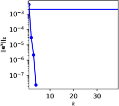
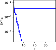
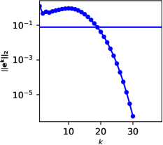
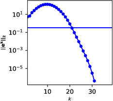
Figure 8: Norm of $\mathbf{e}^{k}$ for the linear advection-diffusion equation with initial value (80) depending on strength of diffusion: $D=1$ (upper left), $D=0.1$ (upper right), $D=0.01$ (lower left) and $D=0$ (lower right). Again the coarse and fine propagator are identical except for the polynomial degree, which is $p=3$ for the fine and $p=2$ for the coarse method. The number of time slices is $P=40$.

5 Conclusions

The paper studies convergence of the parallel-in-time Parareal algorithm for linear initial value problems when spatial coarsening is used. First, the matrix that governs error propagation in the iteration is derived and, assuming the system matrix of the linear initial value problem is normal, a lower bound for the $l_{2}$-norm of the error matrix is derived. Implications of the bound are discussed. In particular, we show how for problems without diffusion the norm of the error matrix must be larger than one when even minimal spatial coarsening is used. While this does not necessarily imply non-convergence in practice, it prevents a theoretical guarantee for monotonic convergence. Furthermore, numerical examples demonstrates that spatial coarsening has a substantial negative impact on convergence for non-diffusive problems. For diffusive problems, the bound is more forgiving and can be smaller than one even when spatial coarsening is used. However, we show in a theoretical toy example and numerical examples that unless convergence is much better than the norm suggests, reaching the discretisation error of the fine method can often take too many iterations to achieve meaningful speedup.

There are two main conclusions that can be drawn. First, care must be taken when reporting speedups for Parareal when spatial coarsening is used. The iteration error can contract more or less at the same rate as the amplitude of the solution due to diffusion (and not at all if there is no diffusion). This means that it is easy to run into situations where reported speedups may be largely because of an unfair comparison [16]. Either the truncated modes on the coarse grid do not contribute to the accuracy of the numerical solution and could have been omitted on the fine mesh as well or the Parareal iteration was stopped too early and the parallel solution is less accurate than the fine reference. Second, the norm of the Parareal error propagation matrix is not necessarily an accurate predictor of actual convergence behaviour, which is a well documented issue for non-normal matrices [19]. For setups where the norm is larger than one, Parareal still often converges even though convergence is mostly poor. Despite these shortcomings, the norm of $\mathbf{E}$ has been used with some success in the analysis of Parareal applied to variations of Dahlquist’s test equation [2, 28]. But the results in this paper suggest that this is unlikely a viable approach to produce a deeper understanding of Parareal in a genuine PDE context where in almost all scenarios some form of spatial coarsening will be needed for good performance. Pseudo-spectra, developed by Trefethen and co-workers [33], might be a useful alternative. An investigation whether the pseudo-spectrum of $\mathbf{E}$ can provide better predictions of Parareal convergence is work in progress. Finally, the derivation of the lower bound strongly relies on the fact that the used interpolation and restriction are linear operators. Machine learning techniques like super-resolution [9] could be used to provide nonlinear transfer operators that might deliver better performance.

References

- [1] P. Amodio and L. Brugnano, Parallel solution in time of ODEs: some achievements and perspectives, Applied Numerical Mathematics, 59 (2009), pp. 424–435, https://doi.org/10.1016/j.apnum.2008.03.024, http://dx.doi.org/10.1016/j.apnum.2008.03.024.
- [2] T. Buvoli and M. L. Minion, Imex parareal integrators. 2020, http://arxiv.org/abs/2011.01604v1.
- [3] J. Dongarra and al., Applied Mathematics Research for Exascale Computing, Tech. Report LLNL-TR-651000, Lawrence Livermore National Laboratory, 2014, {http://science.energy.gov/~/media/ascr/pdf/research/am/docs/EMWGreport.pdf}.
- [4] D. R. Durran, Numerical Methods for Fluid Dynamics, vol. 32 of Texts in Applied Mathematics, Springer-Verlag New York, 2010, http://dx.doi.org/10.1007/978-1-4419-6412-0.
- [5] C. Eckart and G. Young, The approximation of one matrix by another of lower rank, Psychometrika, 1 (1936), pp. 211–218, https://doi.org/10.1007/BF02288367, https://doi.org/10.1007/BF02288367.
- [6] M. Emmett and M. L. Minion, Toward an Efficient Parallel in Time Method for Partial Differential Equations, Communications in Applied Mathematics and Computational Science, 7 (2012), pp. 105–132, https://doi.org/10.2140/camcos.2012.7.105, http://dx.doi.org/10.2140/camcos.2012.7.105.
- [7] R. D. Falgout, S. Friedhoff, T. V. Kolev, S. P. MacLachlan, and J. B. Schroder, Parallel time integration with multigrid, SIAM Journal on Scientific Computing, 36 (2014), pp. C635–C661, https://doi.org/10.1137/130944230, http://dx.doi.org/10.1137/130944230.
- [8] P. F. Fischer, F. Hecht, and Y. Maday, A parareal in time semi-implicit approximation of the Navier-Stokes equations, in Domain Decomposition Methods in Science and Engineering, R. Kornhuber and et al., eds., vol. 40 of Lecture Notes in Computational Science and Engineering, Berlin, 2005, Springer, pp. 433–440, https://doi.org/10.1007/3-540-26825-1_44, http://dx.doi.org/10.1007/3-540-26825-1_44.
- [9] K. Fukami, K. Fukagata, and K. Taira, Machine-learning-based spatio-temporal super resolution reconstruction of turbulent flows, Journal of Fluid Mechanics, 909 (2021), p. A9, https://doi.org/10.1017/jfm.2020.948.
- [10] M. J. Gander, Analysis of the Parareal Algorithm Applied to Hyperbolic Problems using Characteristics, Bol. Soc. Esp. Mat. Apl., 42 (2008), pp. 21–35.
- [11] M. J. Gander, 50 years of Time Parallel Time Integration, in Multiple Shooting and Time Domain Decomposition, Springer, 2015, https://doi.org/10.1007/978-3-319-23321-5_3, http://dx.doi.org/10.1007/978-3-319-23321-5_3.
- [12] M. J. Gander and S. Vandewalle, Analysis of the Parareal Time-Parallel Time-Integration Method, SIAM Journal on Scientific Computing, 29 (2007), pp. 556–578, https://doi.org/10.1137/05064607X, http://dx.doi.org/10.1137/05064607X.
- [13] M. J. Gander and S. Vandewalle, On the Superlinear and Linear Convergence of the Parareal Algorithm, in Domain Decomposition Methods in Science and Engineering, O. B. Widlund and D. E. Keyes, eds., vol. 55 of Lecture Notes in Computational Science and Engineering, Springer Berlin Heidelberg, 2007, pp. 291–298, https://doi.org/10.1007/978-3-540-34469-8_34, http://dx.doi.org/10.1007/978-3-540-34469-8_34.
- [14] C. W. Gear, Parallel methods for ordinary differential equations, CALCOLO, 25 (1988), pp. 1–20, https://doi.org/10.1007/BF02575744, http://dx.doi.org/10.1007/BF02575744.
- [15] N. Gillis and Y. Shitov, Low-rank matrix approximation in the infinity norm, Linear Algebra and its Applications, 581 (2019), pp. 367–382, https://doi.org/10.1016/j.laa.2019.07.017, https://doi.org/10.1016/j.laa.2019.07.017.
- [16] S. Götschel, M. Minion, D. Ruprecht, and R. Speck, Twelve ways to fool the masses when giving parallel-in-time results, in Parallel-in-Time Integration Methods, B. Ong, J. Schroder, J. Shipton, and S. Friedhoff, eds., Cham, 2021, Springer International Publishing, pp. 81–94.
- [17] R. Grone, C. R. Johnson, E. M. Sa, and H. Wolkowicz, Normal matrices, Linear Algebra and its Applications, 87 (1987), pp. 213–225, https://doi.org/10.1016/0024-3795(87)90168-6, https://doi.org/10.1016/0024-3795(87)90168-6.
- [18] E. Hairer and G. Wanner, Solving Ordinary Differential Equations II: Stiff problems, Springer-Verlag Berlin Heidelberg, 1996, http://dx.doi.org/10.1007/978-3-642-05221-7.
- [19] D. J. Higham and L. N. Trefethen, Stiffness of ODEs, BIT Numerical Mathematics, 33 (1993), pp. 285–303, https://doi.org/10.1007/BF01989751, https://doi.org/10.1007/BF01989751.
- [20] R. A. Horn and C. R. Johnson, Topics in Matrix Analysis, Cambridge University Press, 1991.
- [21] R. A. Horn and C. R. Johnson, Matrix Analysis, Cambridge University Press, 2012.
- [22] A. Howse, H. Sterck, R. Falgout, S. MacLachlan, and J. Schroder, Parallel-in-time multigrid with adaptive spatial coarsening for the linear advection and inviscid burgers equations, SIAM Journal on Scientific Computing, 41 (2019), pp. A538–A565, https://doi.org/10.1137/17M1144982, https://dx.doi.org/10.1137/17M1144982.
- [23] C. T. Kelley, Iterative methods for linear and nonlinear equations, Society for Industrial and Applied Mathematics, 1995.
- [24] J.-L. Lions, Y. Maday, and G. Turinici, A ”parareal” in time discretization of PDE’s, Comptes Rendus de l’Académie des Sciences - Series I - Mathematics, 332 (2001), pp. 661–668, https://doi.org/10.1016/S0764-4442(00)01793-6, http://dx.doi.org/10.1016/S0764-4442(00)01793-6.
- [25] A. S. Nielsen, G. Brunner, and J. S. Hesthaven, Communication-aware adaptive parareal with application to a nonlinear hyperbolic system of partial differential equations, Journal of Computational Physics, (2018), https://doi.org/10.1016/j.jcp.2018.04.056, https://doi.org/10.1016/j.jcp.2018.04.056.
- [26] B. W. Ong and J. B. Schroder, Applications of time parallelization, Computing and Visualization in Science, 23 (2020), https://doi.org/10.1007/s00791-020-00331-4, https://doi.org/10.1007/s00791-020-00331-4.
- [27] D. Ruprecht, Convergence of Parareal with spatial coarsening, PAMM, 14 (2014), pp. 1031–1034, https://doi.org/10.1002/pamm.201410490, http://dx.doi.org/10.1002/pamm.201410490.
- [28] D. Ruprecht, Wave propagation characteristics of parareal, Computing and Visualization in Science, 19 (2018), pp. 1–17, https://doi.org/10.1007/s00791-018-0296-z, https://doi.org/10.1007/s00791-018-0296-z.
- [29] J. Schroder, T. Kolev, and V. Dobrev, Multigrid-reduction-in-time with spatial coarsening: A practical and theoretical examination. In preparation, 2021.
- [30] B. S. Southworth, Necessary Conditions and Tight Two-level Convergence Bounds for Parareal and Multigrid Reduction in Time, SIAM J. Matrix Anal. Appl., 40 (2019), pp. 564–608, https://doi.org/https://doi.org/10.1137/18M1226208.
- [31] R. Speck, D. Ruprecht, R. Krause, M. Emmett, M. L. Minion, M. Winkel, and P. Gibbon, A massively space-time parallel N-body solver, in Proceedings of the International Conference on High Performance Computing, Networking, Storage and Analysis, SC ’12, Los Alamitos, CA, USA, 2012, IEEE Computer Society Press, pp. 92:1–92:11, https://doi.org/10.1109/SC.2012.6, http://dx.doi.org/10.1109/SC.2012.6.
- [32] L. N. Trefethen, Finite difference and spectral methods for ordinary and partial differential equations, 1996, http://people.maths.ox.ac.uk/trefethen/pdetext.html. Unpublished text.
- [33] L. N. Trefethen and M. Embree, Spectra and Pseudospectra: The Behavior of Nonnormal Matrices and Operators, Princeton University Press, Princeton and Oxford, 2005.
- [34] S. Vater, N. Beisiegel, and J. Behrens, A limiter-based well-balanced discontinuous galerkin method for shallow-water flows with wetting and drying: One-dimensional case, Advances in Water Resources, 85 (2015), pp. 1–13, https://doi.org/https://doi.org/10.1016/j.advwatres.2015.08.008, https://www.sciencedirect.com/science/article/pii/S0309170815001943.