No detection of SO₂, H₂S, or OCS in the atmosphere of Mars from the first two Martian years of observations from TGO/ACS

Abstract

Context. The detection of sulphur species in the Martian atmosphere would be a strong indicator of volcanic outgassing from the surface of Mars.

Aims. We wish to establish the presence of SO₂, H₂S, or OCS in the Martian atmosphere or determine upper limits on their concentration in the absence of a detection.

Methods. We perform a comprehensive analysis of solar occultation data from the mid-infrared channel of the Atmospheric Chemistry Suite instrument, on board the ExoMars Trace Gas Orbiter, obtained during Martian years 34 and 35.

Results. For the most optimal sensitivity conditions, we determine 1$\sigma$ upper limits of SO₂ at 20 ppbv, H₂S at 15 ppbv, and OCS at 0.4 ppbv; the last value is lower than any previous upper limits imposed on OCS in the literature. We find no evidence of any of these species above a 3$\sigma$ confidence threshold. We therefore infer that passive volcanic outgassing of SO₂ must be below 2 ktons/day.

1 Introduction

Multiple pieces of evidence point to the presence of substantial past volcanic activity on Mars. This activity may in fact have been key in maintaining a sufficiently warm, dense, and moist palaeoclimate through greenhouse gas emission, thus allowing for a stable presence of surface liquid water (e.g. Craddock & Greeley, 2009). While this past activity is partly reflected in gaseous isotope ratios that are found in the present-day Martian atmosphere (Jakosky & Phillips, 2001; Craddock & Greeley, 2009), more obvious evidence is provided by the numerous large volcanic structures and lava flows present over much of the surface of Mars that have been studied since the first spacecraft observations made by the Mariner 9 orbiter in the 1970s (Masursky, 1973). Evidence of present-day outgassing activity on Mars, however, remains more elusive. While no signs of thermal hotspots were found by the Mars Odyssey/Thermal Emission Imaging System (THEMIS) instrument (Christensen et al., 2003), evidence from the Mars Express/High Resolution Stereo Camera (HRSC) showed signs of very intermittent activity from volcanoes that erupt between periods of dormancy that last for hundreds of millions of years around the Tharsis and Elysium regions (Neukum et al., 2004), with the most recent activity in some cases dating from only a few million years ago. More recently, the InSight Lander found that seismic activity was generally lower than expected on Mars; however, the two largest marsquakes it managed to detect were in the Cerberus Fossae region (Giardini et al., 2020). This was later accompanied by evidence from the Mars Reconnaissance Orbiter/High Resolution Imaging Experiment (HIRISE) of extremely recent volcanic activity in the same region dating back only around 100,000 years (Horvath et al., 2021).This gives further credence to the possibility of residual volcanic activity continuing to the present day, perhaps from localised thermal vents.

On Earth, sulphur dioxide (SO₂) tends to be by far the most abundant compound emitted through passive volcanic degassing after CO₂ and water vapour; it is detected together with smaller amounts of hydrogen sulphide (H₂S) and occasionally carbonyl sulphide (OCS), although the exact ratios of these compounds usually depend on the volcano and the type of eruption or outgassing in question (Symonds et al., 1994). Gaillard & Scaillet (2009) used constraints on the composition of Martian basalts, together with thermochemical constraints on the composition of the Martian mantle, to estimate a sulphur content of potential Martian volcanic emission, especially from volcanoes that formed later in Mars’ history, such as those in the Tharsis range, which is 10 - 100 times higher than equivalent sulphur emission from Earth volcanoes. Since these sulphurous gases have stabilities in the Martian atmosphere of the order of only days to a few years (Nair et al., 1994; Krasnopolsky, 1995; Wong et al., 2003, 2005), their detection in the Martian atmosphere would be a strong indicator of residual present-day volcanic activity on Mars. Alternatively, it could be a sign of a coupling between the atmosphere and sulphur-containing regoliths (Farquhar et al., 2000) or sulphate deposits that are present in multiple regions of Mars (Bibring et al., 2005; Langevin et al., 2005). This would be an indirect sign of past volcanic activity but one that would nonetheless shed light on a previously unknown sulphur cycle in the Martian atmosphere.

Recent detections of other new trace gases in the atmosphere of Mars from remote sensing provide a tantalising glimpse of fascinating new Martian surface and atmospheric chemistry that until now had remained unknown to science. Examples include the independent detections of hydrogen peroxide by Clancy et al. (2004) and Encrenaz et al. (2004), a photochemical product that acts as a possible sink for organic compounds in the atmosphere; and the independent detections of hydrogen chloride (HCl) reported by Korablev et al. (2021), Olsen et al. (2021c), and Aoki et al. (2021), a possible tracer of the interaction of dust with the atmosphere. HCl in particular was historically assumed to be a tracer of volcanic outgassing and was hypothesised to be responsible for the observed geographical distribution of elemental chlorine (Keller et al., 2006) and perchlorates (Hecht et al., 2009; Catling et al., 2010). While the seasonality of observed HCl detections in the Martian atmosphere has made a volcanic origin less likely, more recent anomalous detections of HCl in aphelion reported by Olsen et al. (2021c) have not entirely ruled it out. We should of course also note various disputed detections of methane (e.g. Formisano et al., 2004; Krasnopolsky et al., 2004; Mumma et al., 2009; Webster et al., 2015), whose ultimate provenance remains subject to debate and could be a result of a number of different processes, including volcanic outgassing (Oehler & Etiope 2017; and references therein), but whose legitimacy has been seriously questioned by recent satellite measurements (Korablev et al., 2019; Montmessin et al., 2021).

Despite this, all attempts to constrain the presence of sulphurous gases in the Martian atmosphere, and in particular SO₂, have failed to confirm any statistically significant positive detections. Although comprehensive searches for trace gases in the Martian atmosphere have been ongoing since the Mariner 9 era (Maguire, 1977), most of the earliest attempts were hampered by the lack of spectral sensitivity and low spectral resolution: the resolving power in the mid-infrared where many of the required spectral signatures are located generally needs to be greater than 10,000 in order to resolve them from neighbouring CO₂ and H₂O absorption lines. More recent literature concerning upper limits relied on ground-based observations that were made at much higher spectral resolutions, with SO₂ and H₂S spectral data obtained in the sub-millimetre (e.g. Nakagawa et al., 2009; Encrenaz et al., 2011) and the thermal infrared (Krasnopolsky, 2005, 2012) wavenumber ranges, and corresponding OCS spectral data around an absorption band in the mid-infrared (Khayat et al., 2017). However, ground-based observations still have a number of drawbacks. Firstly, they are hindered by a lack of temporal coverage. Secondly, the presence of telluric absorption in ground-based observations also obscures gas absorption signatures of Martian provenance, removal of which requires correction for Doppler shift (cited by Zahnle et al. 2011 as a possible source of false detections of methane) as well as a complex radiative transfer model that decouples the contribution from Earth and Mars. Finally, they can often lack the spatial resolution necessary to resolve local sources of emission. By contrast, observations from probes in orbit suffer less from these issues and have more localised spatial coverage, which enabled the recent detection of HCl in orbit despite numerous recent failed attempts to detect it from the ground, even with instruments of similar spectral resolution (e.g. Krasnopolsky et al., 1997; Hartogh et al., 2010; Villanueva et al., 2013).

In this work we present upper detection limits on SO₂, H₂S, and OCS based on spectral data from the first two Martian years of observations from the mid-infrared channel of the Atmospheric Chemistry Suite instrument (ACS MIR; Korablev et al., 2018) on board the ExoMars Trace Gas Orbiter (TGO; Vago et al., 2015). In Sect. 2 we introduce the ACS MIR data and summarise the data calibration process, and in Sect. 3 we present the two methods used to establish detection limits on each of the given compounds. In Sect. 4 we present the retrieved upper limits for each of the sulphur trace species in turn. Discussion and conclusions are reserved for Sect. 5.

2 Data and calibration

TGO has been in orbit around Mars since October 2016 and has operated continuously since the start of its nominal science phase in April 2018, providing a wealth of data covering one and a half Martian years as of writing (from L_s= 163° in MY 34 to L_s= 352° in MY 35). On board are two sets of infrared spectrometers designed to perform limb, nadir, and solar occultation observations of the atmosphere: the ACS (Korablev et al., 2018) and the Nadir and Occultation for Mars Discovery (NOMAD; Vandaele et al., 2018) instruments. In this work, we focus on the ACS MIR instrument (Trokhimovskiy et al., 2015), which observes Mars purely through solar occultation viewing geometry with the line of sight parallel to the surface, obtaining a set of transmission spectra of the Martian atmosphere at individual tangent heights separated at approximately 2 km intervals from well below the surface of Mars up to the top of the atmosphere during a single measurement sequence. The closer the tangent height of observation to the surface, the greater the molecular number density of the absorbing species and hence the greater the optical depth integrated along the line of sight. This allows for higher sensitivities to very small abundances of trace gases, in theory down to single parts per trillion for some species (Korablev et al., 2018; Toon et al., 2019), than can be achieved from ground-based observations where the path length through the atmosphere is much shorter. In practice, however, the sensitivity is limited by instrumental noise and artefacts, and the signal-to-noise ratio (S/N) usually decreases at lower altitudes due to the attenuation of the solar signal by the presence of dust, cloud and gas absorption. The best upper limits for trace gas species are therefore usually obtained as close to the surface as possible under very clear atmospheric conditions, which occur especially near the winter poles, during aphelion and excluding global dust storm periods.

ACS MIR is a cross-dispersion echelle spectrometer that covers a spectral range of 2400-4500 cm^-1 with a spectral resolving power of up to 30,000 (Trokhimovskiy et al., 2020). The instrument makes use of a steerable secondary reflecting grating that then disperses the incoming radiation and separates it into named diffraction orders that encompass smaller wavenumber subdivisions. The group of diffraction orders that is selected depends on the position of the secondary grating. In this work we analyse observations obtained using three grating positions: position 9, which covers the main SO₂ absorption bands; position 11, which covers the strongest OCS absorption bands; and position 5, which covers H₂S. Respectively, these grating positions cover wavenumber ranges of 2380 - 2560 cm^-1 (diffraction orders 142 - 152), 2680 - 2950 cm^-1 (160 - 175), and 3780 - 4000 cm^-1 (226 - 237). In each case, only one grating position is used per measurement sequence and the spatial distribution of these measurements over the time period covered in this analysis is shown in Fig. 1. The end product is a 2D spectral image from each tangent height projected onto a detector, which consists of wavenumbers dispersed in the x axis and diffraction orders separated along the y axis (the reader is directed to Korablev et al. (2018); Trokhimovskiy et al. (2020); Olsen et al. (2021a); Montmessin et al. (2021) for diagrams and further discussion). This image contains approximately 20 - 40 pixel rows per diffraction order depending on the grating position in question, corresponding to an increment of around 200 - 300 m in tangent height per row. The intensity distribution of incoming radiation is distributed asymmetrically over each diffraction order, with the row of maximum intensity, and hence maximum S/N, usually located somewhere between the geometric centre of the diffraction order and the edge of the slit that is over the solar disc.

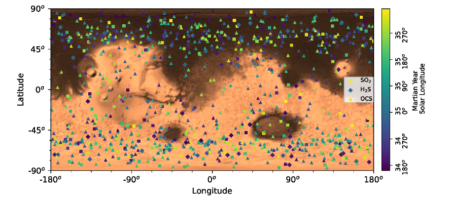
Figure 1: Spatial and temporal distribution of all the ACS MIR observations covered in this analysis. Squares represent observations made by ACS using grating position 9 (sensitive to SO₂), diamonds using grating position 5 (H₂S), and triangles using grating position 11 (OCS). The colour of each symbol represents the time, in units of solar longitude ($L_{s}$) over Martian years (MY) 34 and 35, at which the observation was obtained. The relative concentration of observations made closer to the poles is due to the TGO orbital geometry. Latitude values are planetocentric. The background image of Mars is based on topography data from the Mars Orbiter Laser Altimeter (MOLA) instrument on board Mars Global Surveyor (Smith et al., 2001).

We should also note the presence of ‘doubling’, an artefact of unknown origin that causes two images per tangent height, offset horizontally and vertically by a few pixels, to be projected onto the detector surface, resulting in transmission spectra in which each absorption line appears to be divided into two separate local minima (Alday et al., 2019; Olsen et al., 2021a). This doubling effect tends to be strongest in the centre of the illuminated portion of the slit where the signal strength is highest, and its profile changes across each row of a given diffraction order in ways that are still under investigation as of writing. In practice it also acts to reduce the effective spectral resolution of ACS MIR spectra from the nominal value (Olsen et al., 2021c) and hence proves a major source of error in the determination of upper limit values.

Calibration was performed according to the procedure detailed in Trokhimovskiy et al. (2020) and Olsen et al. (2021a). Observations in the measurement sequence when the field-of-view is fully obscured by Mars were used to estimate dark current and thermal background. At the other end of the measurement sequence, observations in the very high atmosphere were used to estimate the solar spectrum, taking account the drift of the image on the detector over time induced by the thermal background. Stray light was estimated from the signal level between adjacent diffraction orders. A first guess of the pixel-to-wavenumber registration was made by comparing the measured solar spectrum with reference solar lines (Hase et al., 2010), which was then further refined as part of the retrieval process as will be described in Sect. 3.1. The tangent height of each observation at the edges of the slit was estimated using the TGO SPICE kernels (Trokhimovskiy et al., 2020), where the row positions of the top and bottom of each slit were established using reference ‘sun-crossing’ measurement sequences in which the slit passes across the Sun perpendicularly to the incident solar radiation path above the top of the atmosphere. Nonetheless, there is still some uncertainty on the tangent height registration as a) although we assume a linear distribution, the change in tangent height over each intermediate slit row is not well constrained and b) the pixel offset between the two doubled images can make it difficult to identify the exact locations of the slit edges on the detector array. This uncertainty is usually of the order of around 0.5 - 1.0 km.

3 Analysis

3.1 RISOTTO forward model

Upper limits are obtained using the RISOTTO radiative transfer and retrieval pipeline (Braude et al., 2021). RISOTTO relies on Bayesian optimal estimation, starting from a prior state vector of parameters relating both to the atmospheric quantities that we wish to retrieve from the data (in this case, vertical gas abundance profiles quantified in units of volume mixing ratio, hereon abbreviated to VMR) and a number of instrumental parameters intended to reduce systematic errors due to noise, uncertainties in instrumental calibration or the presence of aerosol. We model three of these instrumental parameters specifically: first, a polynomial law that relates the first guess of the pixel-to-wavenumber registration to a more accurate registration; second, an instrument line shape model akin to that described by Alday et al. (2019) that approximates the doubling artefact observed in spectra from ACS MIR; and third, the transmission baseline as a function of wavenumber that takes into account broad variations in the shape of the spectrum while simultaneously avoiding problems of so-called overfitting, where any narrow residuals due to individual noise features or poorly modelled gas absorption lines are compensated for by changing the baseline in an unphysical manner. The algorithm then computes a forward model based on these parameters and then iteratively finds the optimal values of both the scientific quantities and the instrumental parameters simultaneously that best fit the observed transmission spectra, together with their associated uncertainties. In order to model gas absorption along the line of sight both accurately and in a manner that is computationally efficient, spectral absorption cross-section lookup tables are calculated from the HITRAN 2016 database (Gordon et al., 2017) over a number of sample pressure and temperature values that reflect the range of values typically found in the Martian atmosphere, and then a quartic function is derived through regression to compute the cross-sections at any given intermediate pressure and temperature value as explained further in Braude et al. (2021). Examples of these computed cross-sections for each of the three molecules studied in this article are shown in Fig. 2a-c, with the corresponding wavenumber selections for the retrievals set to favour stronger molecular lines while avoiding lines that overlap too greatly with lines of other known molecules present in the region. As an illustration of how these species may appear in real ACS MIR spectra given predicted abundances, Fig. 2d-i show equivalent approximate simulated transmissions for the major species in the spectral ranges present in the three orders, with conditions equivalent to those near the south pole at aphelion around 10 km of altitude, and convolved with a Gaussian instrument line shape function of R $\sim$ 20,000 to roughly reflect the reduction in spectral resolution due to doubling. For both figures we assume an atmosphere of 95.5% CO₂, 100 ppmv H₂O, 10 ppbv of SO₂ and H₂S, and 1 ppbv of HCl and OCS, corresponding either to simulated detection limits in optimal dust conditions (Korablev et al., 2018) or existing measurements of known species (eg. Fedorova et al. 2020; Korablev et al. 2021). We can see that the regions in which the strongest SO₂ and H₂S lines are located are dominated by much stronger lines of CO₂ and H₂O. By contrast, the spectral region in which OCS is found is usually much clearer, with HCl absorption lines easily resolvable and only found during certain seasons.

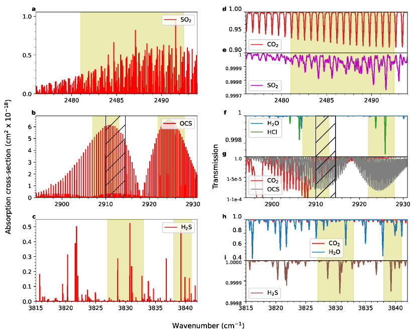
Figure 2: Computed cross-section values and simulated transmission spectra, for illustrative reference pressure and temperature values of 1 mbar and 200 K, respectively. Displayed wavenumber ranges reflect the coverage of the analysed diffraction orders, with the light yellow highlighted regions showing the spectral intervals over which detection limit retrievals were conducted, maximising absorption from the trace species in question while minimising overlapping absorptions from other known species. Panels a-c: Cross-section values for (a) SO₂ in diffraction order 148, (b) OCS in diffraction orders 173 and 174, and (c) H₂S in diffraction order 228. The grey cross-hatched regions in panels (b), (f), and (g) show the wavenumber range overlap between diffraction order 173 on the left and diffraction order 174 on the right. Panels d-i: Estimated transmission spectra given the aforementioned pressure and temperature conditions, convolved with a Gaussian instrument function of resolution R $\sim$ 20,000. For each diffraction order, we plot the contributions of the trace species to the total transmission separately from the other interfering species, for which the contribution is several orders of magnitude larger.

At the wavenumber ranges studied in this analysis, the CO₂ absorption lines are not usually strong enough to independently constrain gaseous abundances, temperature and pressure all simultaneously. This can be even further exacerbated by uncertainties induced by systematic errors in the instrument line shape due to doubling (e.g. Alday et al., in review). Nonetheless, retrieved gas abundances are heavily degenerate with temperature and pressure and so completely arbitrary values cannot be chosen. A priori temperature and pressure data are therefore usually sourced from fitting stronger CO₂ bands in the near-infrared (NIR) channel of ACS data obtained during the same measurement sequence (Fedorova et al., 2020). For occasional ACS measurement sequences, however, these observations are not available, in which case we use estimates from the Laboratoire de Météorologie Dynamique general circulation model (LMD GCM) solar occultation database (Forget et al., 1999; Millour et al., 2018; Forget et al., 2021), which computes vertical profiles of a number of atmospheric parameters for the given time and location of an ACS measurement sequence using a GCM. For retrievals where no CO₂ bands are to be fitted, such as with OCS, it is usually adequate to leave the temperature-pressure profile fixed in the retrieval. For retrievals of SO₂ and H₂S where they are to be fitted, the LMD GCM estimates are not always close enough to the true value to provide a good fit to the CO₂ absorption bands, and so minor adjustments in the temperature-pressure profile do have to be made in the retrieval. To decouple the effects of temperature and pressure, we keep a reference pressure value at a given altitude fixed to that from the LMD solar occultation database, then use the CO₂ bands to retrieve a vertical temperature profile directly from the data and thereby derive a vertical pressure profile by assuming hydrostatic equilibrium (e.g. Quémerais et al., 2006; Alday et al., 2019, 2021; Montmessin et al., 2021).

3.2 Retrieval procedure

3.2.1 H₂S and OCS

A number of approaches can be used to derive the upper limit of detection of a given species, each with their advantages and disadvantages. The most common approach is to define the upper limit as the estimate of the uncertainty on a retrieved VMR given a true VMR equal to 0; if the retrieved VMR was greater than this uncertainty value, it would be deemed a detection as opposed to an upper limit. This uncertainty can be estimated either by quantifying each of the sources of error in turn (e.g. Aoki et al., 2018) or by deriving a first estimate of the uncertainty from a retrieval code and then adjusting the uncertainties post hoc according to statistical criteria (e.g. Montmessin et al., 2021; Knutsen et al., 2021). This method is expanded on by Olsen et al. (2021b) by performing an independent retrieval of the vertical gas profiles using multiple pixel rows on the ACS MIR detector array, and then calculating an upper limit value from the standard error on the weighted average of the vertical profiles from each of these retrievals combined. This has the added benefit of increasing the statistical significance of a measurement through repeated observation and thereby deriving lower upper limits.

For retrievals of upper limits of OCS and H₂S, we use a modified version of the Olsen et al. (2021b) method, but with some further amendments to minimise uncertainties in the estimated spectral noise level, as well as to reduce sensitivity due to intrinsic biases imposed either by the prior state vector or by local artefacts in the spectrum. The sigma detection value at each altitude is determined by the ratio of the weighted mean abundance value $\mu_{j}^{*}$ to the weighted standard deviation $\varsigma_{j}^{*}$ as found by the procedure detailed in Appendix A, that is to say, where $\mu_{j}^{*}/\varsigma_{j}^{*}=1$ indicates a positive 1$\sigma$ detection. Usually, a 1$\sigma$ or 2$\sigma$ detection indicates overfitting of local artefacts or noise features as opposed to a genuine positive detection. We therefore treat anything below a 3$\sigma$ detection as insignificant and define our upper limit at each altitude by adding total sources of both systematic and random error in quadrature, that is to say, the upper limit is equal to $\sqrt{\mu_{j}^{*2}+\varsigma_{j}^{*2}}$ smoothed using a narrow Gaussian filter with respect to altitude, as shown in Fig. 3.

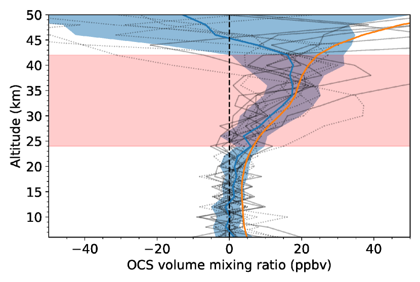
Figure 3: Illustrative example of the upper limit derivation methodology for OCS and H₂S. Grey lines indicate the individual $2N$ vertical profiles of OCS retrieved according to (solid) step 3 and (dotted) step 4, for each row on the detector array. The solid blue line shows the weighted mean abundance profile, $\mu_{j}^{*}$, derived from the individual retrievals, with the standard deviation, $\varsigma_{j}^{*}$, shown in the shaded blue region. The solid orange line shows the profile of $\sqrt{\mu_{j}^{*}+\varsigma_{j}^{*}}$ smoothed over altitude. The red shaded region shows the altitude range for which a 1$\sigma$ detection was determined, i.e. where the value of $\varsigma_{j}^{*}$ is lower than the value of $\mu_{j}^{*}$.

3.2.2 SO₂

Retrievals of SO₂ are complicated by the fact that SO₂ has a dense line structure that is difficult to fully resolve at the given spectral resolution, and so retrievals of SO₂ are somewhat difficult to decouple from uncertainties in the baseline level induced by noise, calibration errors, and aerosol extinction. Failure to take into account uncertainties in the baseline level will therefore result in upper limits of SO₂ that are too low. While RISOTTO should ordinarily be able to handle some degeneracy with low frequency baseline variations (Braude et al., 2021) that would save having to perform a more complicated fitting procedure as in Belyaev et al. (2008, 2012) to fully separate out the contribution of aerosol and SO₂ to the continuum absorption, the situation is made complicated by the presence of artefacts near the edge of the detector where the degeneracy between low-frequency baseline variations and SO₂ absorption can most easily be broken due to the presence of prominent SO₂ lines. The retrieval code therefore has the propensity of overfitting artefacts, resulting in false detections of highly negative abundances of SO₂.

One method is to start with a forward model where the species is absent, and gradually inject incrementally large quantities of the species into the forward model until the change in the spectral fit is deemed to increase above a given threshold (eg. Teanby et al., 2009; Korablev et al., 2021). In practice this can become slow and unwieldy in the case of solar occultations where there are multiple spectra to be fit simultaneously, each with their own independent noise profile and sensitivity to the given species. In addition, it also begs the question as to how the threshold should be defined quantitatively, especially if the S/N is uncertain.

Teanby et al. (2009) assessed the significance of a detection according to the mean squared difference between the observed spectrum $y_{obs}(\nu)$ as a function of wavenumber, $\nu$, and the modelled spectrum $y_{mod}(\nu,x)$ given an ‘injected’ gas volume mixing ratio, $x$, weighted according to the spectral uncertainty $\sigma(\nu)$:

$$\Delta\chi^{2} =\chi^{2}(x)-\chi^{2}(0)$$ (1)

$$=\sum_{i}^{N_{\nu}}\left(\left(\frac{y_{obs}(\nu_{i})-y_{mod}(\nu_{i},x)}{\sigma(\nu_{i})}\right)^{2}-\left(\frac{y_{obs}(\nu_{i})-y_{mod}(\nu_{i},0)}{\sigma(\nu_{i})}\right)^{2}\right),$$ (2)

where $N_{\nu}$ is the number of individual spectral points in a given observation. The residual errors on the fit to the spectrum are assumed to follow a double exponential distribution (Press et al., 1992), neglecting systematic errors:

$$P(y_{obs}(\nu_{i})-y_{mod}(\nu_{i},0))\sim\exp\left(\;\;\left|\frac{y_{obs}(\nu_{i})-y_{mod}(\nu_{i},0)}{\sigma(\nu_{i})}\right|\;\;\right).$$ (3)

Teanby et al. (2009, 2019) then defined upper limits according to the confidence interval around the mean of the probability distribution described by Eq. 3, so that values of gas abundance $x$ that give a value of $\Delta\chi^{2}=n^{2}$ should represent an n-sigma upper limit, while a gas abundance that results in $\Delta\chi^{2}=-n^{2}$ should analogously represent a positive n-sigma detection. However, this method was used for single isolated lines where the detection limit is more or less independent of the size of the spectral window. This is not the case for SO₂, which has a dense line structure that affects the shape of the baseline, and where there is substantial uncertainty on the values of $\sigma(\nu_{i})$ induced by various sources of systematic error, notably from the doubled instrument line shape. We find in our own data that values of $\Delta\chi^{2}=1$ give detection limits that are far too optimistic even when correcting for spectral sampling as in Teanby et al. (2019). Instead, we find that taking the standard deviation of the double exponential distribution provides more realistic detection limits, which would therefore correspond to n-sigma upper limits and detections of, respectively, $\Delta\chi^{2}=\pm\sqrt{2N_{\nu}}n^{2}$. Depending on the occultation in question, $\sqrt{2N_{\nu}}$ is usually equal to around 25 for the wavenumber range taken into account in the retrieval.

We first performed an initial retrieval where SO₂ is not present in the forward model, only retrieving the temperature profile and the three instrumental parameters as previously described, to give a spectral fit $y_{mod}(\nu,0)$. The values of $\sigma(\nu)$ are then estimated by taking a moving average of the difference between $y_{obs}(\nu)$ and $y_{mod}(\nu,0)$, thereby providing a first guess of spectral uncertainties due to systematics in the spectra and forward modelling error, and hence allowing a preliminary value of $\chi^{2}(0)$ to be calculated. Fixed vertical profiles of SO₂ abundance $x$ were then added to the forward model, and a new retrieval performed where the baseline is allowed to vary but the remaining parameters of the state vector are fixed to those retrieved from $y_{mod}(\nu,0)$. If this results in a value of $\Delta\chi^{2}$ at a given tangent height that is negative, the values of $\sigma(\nu)$ are further refined by taking a moving average of the difference between $y_{obs}(\nu)$ and $y_{mod}(\nu,x)$, so that the contribution of forward modelling error to the spectral uncertainty is minimised. Once enough different vertical profiles of SO₂ were modelled to sufficiently sample the $\Delta\chi^{2}$ parameter space, the approximate 1$\sigma$ level at each altitude was found through progressive quadratic interpolation to a volume mixing ratio profile where $\Delta\chi^{2}$ is as close to $\sqrt{2N_{\nu}}$ as possible for each altitude, or conversely where $\Delta\chi^{2}$ is as low as possible. Due to the presence of systematic errors, we do not attempt to reduce upper limits by adding the contribution of multiple rows of each diffraction order as with H₂S or OCS, instead only analysing a single row close to the centre of the diffraction order that receives the most input radiance and hence has the highest S/N.

4 Results

4.1 SO₂

Given that volcanic emissions of SO₂ are predicted to dwarf those of any other sulphur species and have the longest photochemical lifetime, SO₂ is the tracer that has attracted the most attention in the literature out of all the three gases analysed here. Ground-based observations of SO₂ in the past have focussed on two main spectral regions. In the sub-millimetre there is a single line present at 346 GHz, from which disc-integrated upper limits of 2 ppbv were derived by Nakagawa et al. (2009) and upper limits of just over 1 ppbv by Khayat et al. (2015, 2017). A number of rotational-vibrational lines are also present in the thermal infrared between 1350 - 1375 cm^-1 (Encrenaz et al., 2004, 2011; Krasnopolsky, 2005, 2012), with upper limits of 0.3 ppbv independently confirmed by both Encrenaz et al. (2011) and Krasnopolsky (2012). By contrast, the strongest SO₂ absorption band in the ACS MIR wavenumber range, centred around 2500 cm^-1, is still weaker than the absorption bands found in these two regions. In addition, the SO₂ absorption band has a very dense line structure, which at ACS MIR resolution results in only a small number of isolated lines that are sufficiently prominent to decouple the contributions of SO₂ absorption to the spectrum from the uncertainty in the transmission baseline. This is also further complicated by the fact that several lines overlap strongly with the absorption bands of three separate isotopes of CO₂, several of which are also difficult to resolve from one another and contribute to the baseline uncertainty. The SO₂ line that is best resolved from the baseline and CO₂ absorption is present at 2491.5 cm^-1, but this is also located close to the edge of the diffraction order where the S/N starts to decrease.

We performed retrievals on a relatively broad spectral range of 2481 - 2492 cm^-1, which allowed the strongest lines of ¹²C¹⁶O¹⁸O to be fit in order to constrain both the vertical temperature profile and the doubling line shape, as well as minimising the probability of local noise features at 2491.5 cm^-1 being overfit with SO₂ absorption, while avoiding lower wavenumbers where the contribution of ¹²C¹⁶O¹⁶O and ¹²C¹⁶O¹⁷O to the uncertainty in the transmission baseline starts to become significant. In addition, we also only fit spectra up to a tangent height of 50 km above the Martian geoid (usually referred to as the ‘areoid’) as noise features start to dominate in spectra above this level, which can occasionally be confused with genuine SO₂ absorption by the retrieval code. This is justified as SO₂ emitted from the surface would only be detectable at very high abundances above 50 km as we show later in this section.

We retrieved estimates of upper limits of SO₂ from all measurement sequences obtained using grating position 9 for which the observed altitude of aerosol saturation was below 50 km, according to the procedure previously outlined in Sect. 3.2.2. 190 occultations in total satisfied this criterion, covering a time period of L_s = 165 - 280° of MY 34 and L_s = 140 - 350° of MY 35, in both cases equivalent to the time around perihelion and approaching early aphelion. Occasionally, vertical correlations between spectra, together with the breakdown in the approximation of a quadratic relationship between volume mixing ratio and $\Delta\chi^{2}$ due to baseline degeneracy, can result in failure to converge to a $\Delta\chi^{2}\approx\sqrt{2N_{\nu}}$ solution for certain tangent heights. The altitude ranges at which these poor $\Delta\chi^{2}$ solutions are found are therefore removed from the upper limit profiles before they are smoothed. In Fig. 4, we plot the smoothed vertical upper limit profiles retrieved from all 190 occultations as a function of altitude. We find in most cases that we can derive upper limits down to around 30 - 40 ppbv, usually around 20 km above the areoid, with the sensitivity decreasing exponentially with altitude until only measurements of the order of 1 ppmv of SO₂ are retrievable in the lower mesosphere. Below the 20 km level, the presence of aerosols usually lowers the S/N to the point where the CO₂ lines become heavily distorted, particularly below around 10 - 15 km, which makes accurate fitting of SO₂ very difficult even when taking temperature variations and spectral doubling into account. We find no significant detections of SO₂ to greater than 1$\sigma$ confidence.

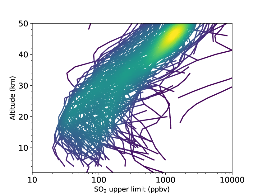
Figure 4: 1$\sigma$ upper limit values of SO₂ obtained as a function of altitude for each position 9 measurement sequence. Yellower colours indicate greater densities of upper limit values for a given altitude.

In Fig. 5 we plot the lowest upper limits retrieved per occultation as a function of altitude and latitude. For reference, we mark periods of increased dust storm activity during perihelion, which usually consists of a large dust storm event that affects the general latitude range between 60° S and 40° N and peaking around $L_{s}=220\text{\textdegree}-240\text{\textdegree}$ , followed by a dip in dust activity just after solstice and a smaller regional dust storm event around $L_{s}=320\text{\textdegree}$ that mostly affects southern mid-latitudes (Wang & Richardson, 2015; Montabone et al., 2015). Dust activity was particularly intense in MY 34 compared with MY 35 (Montabone et al., 2020; Olsen et al., 2021c), and although the poles remained relatively clear of dust even during the MY 34 global dust storm event we were only able to get upper limits down to around 50 ppbv in northern polar regions. By contrast, outside the perihelion dust storm events, the atmosphere could be probed deep enough to attain sufficient sensitivity to regularly attain 1$\sigma$ upper limits of 20 ppbv down at around 10 km above the areoid, close to both the northern and southern polar regions.

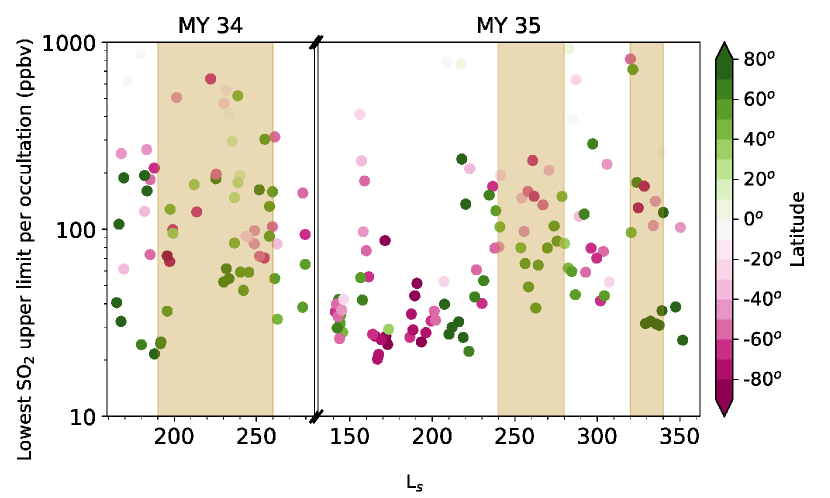
Figure 5: Change in the distribution of the lowest SO₂ upper limit values derived from each ACS occultation sequence as a function of season, with the colour of each circle representing the approximate latitude value where the measurement was obtained. Brown shaded regions indicate major dust storm events (Montabone et al., 2020; Olsen et al., 2021c).

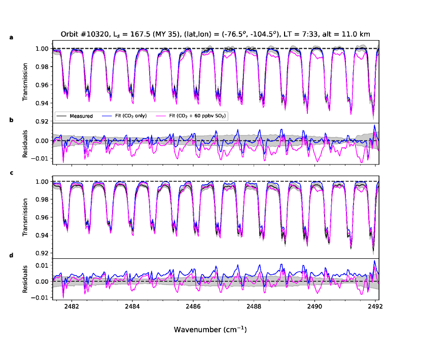
Figure 6: Example fit to a position 9 spectrum for which the lowest upper limits were retrieved from the entire position 9 dataset. In blue is shown the fit to the measured spectrum taking only CO₂ absorption and instrumental parameters into account, with the synthetic spectrum showing the additional contribution of 60 ppbv of SO₂, corresponding to the perceived 3$\sigma$ level, superimposed in magenta. Estimated spectral uncertainty is shaded in grey. All spectra are normalised to the retrieved transmission baseline at unity for clarity. Panels a-b: Spectral fit when the transmission baseline is retrieved only for the initial fitting of the CO₂ lines with zero SO₂ abundance. Panels c-d: Spectral fit when the transmission baseline is re-retrieved following the addition of 60 ppbv of SO₂ into the forward model.

The spectrum where we were able to find the best upper limit value of 20 ppbv is shown in Fig. 6, where we compare the fit using a fixed abundance of SO₂ in the forward model that is equal to 3 times the derived 1 sigma upper limit, to the corresponding fit where no SO₂ is taken into account in the forward model. The change in the aforementioned doubling effect over the breadth of the diffraction order is clearly seen in Fig. 6, with each CO₂ absorption line exhibiting two local absorption minima where the right minimum progressively dominates more over the left minimum as one moves towards the right edge of the detector. The uncertainty induced by this doubling effect on the transmission baseline ensures that the transmission baseline is difficult to derive a priori without knowledge of SO₂ abundance, and this is shown clearly in Panel a of Fig. 6 where fixing the baseline ensures that given abundances of SO₂ result in SO₂ absorption lines that penetrate further out of the noise level than if the baseline is allowed to vary as in Panel c, and hence results in deceptively low SO₂ upper limits. A better-constrained transmission baseline would result in upper limits that are approximately halved, which is also reflected in quoted theoretical upper limits in the literature of 7 ppbv assuming low dust conditions (Korablev et al., 2018). These are still far higher than the aforementioned upper limits of 0.3 - 2 ppbv retrieved from stronger absorption bands in the thermal infrared and the sub-millimetre. Since the uncertainties in the retrievals of SO₂ are so heavily dominated by sources of systematic error, we cannot analyse multiple rows of the detector array in order to reduce these values further. SO₂ is predicted to be well mixed in the atmosphere below 30 - 50 km altitude after approximately six months, depending on the volume of outgassing (Krasnopolsky, 1993, 1995; Wong et al., 2003), well below the predicted photochemical lifetime of 2 years (Nair et al., 1994; Krasnopolsky, 1995). We therefore find that we can still probe to deep enough altitudes for any large surface eruption of SO₂ to be monitored from ACS MIR data within months of its occurrence and be able to track its origin.

4.2 H₂S

Despite lower predicted outgassing rates of H₂S compared with SO₂, and hence a lower likelihood of detectability, the concurrent detection of H₂S is important for three main reasons. Firstly it is a superior tracer of the location of outgassing from the surface due to its shorter photochemical lifetime, with quoted values ranging from of the order of a week (Wong et al., 2003, 2005) to 3 months (Summers et al., 2002), well below the timescales for global mixing in the atmosphere of Mars. Secondly, the H₂S/SO₂ ratio provides additional information on the temperature and water content of an outgassing event, as it is governed by a redox reaction in which a lower temperature and higher water content favours the production of H₂S from SO₂ (Oppenheimer et al. 2011; and references therein). Finally, H₂S is, in itself, a gas that is produced biotically on Earth through the metabolism of sulphate ions in acidic environments (Bertaux et al., 2007), which could hypothetically be produced by micro-organisms living in sulphate deposits on Mars.

Even the strongest H₂S lines in the ACS MIR wavenumber range are relatively weak, with maximum HITRAN 2016 line strengths of $\sim$1.6 x 10^-21cm^-1/(molecule cm^-2) at 296 K, compared with equivalent lines found in the thermal infrared at 1293 cm^-1($\sim$3.3 x 10^-20 cm^-1/(molecule cm^-2); Maguire, 1977; Encrenaz et al., 2004) and especially with lines in the sub-millimetre ($\sim$4.6x 10^-20 cm² GHz; Pickett et al. 1998; Encrenaz et al. 1991; Khayat et al. 2015). In addition, the spectral region in which most H₂S absorption lines are found is dominated by the absorption of several different isotopologues of CO₂ and H₂O (Alday et al., 2019), with especially strong absorption by H₂¹⁶O. We focus here on one particular spectral region between 3827 - 3833 cm^-1 around some of the strongest H₂S bands in the ACS MIR wavenumber range, located in diffraction order 228 of grating position 5, as well as an additional spectral window around a single strong line at 3839.2 cm^-1 located near the edge of the diffraction order where the S/N is lowest. Temporal coverage for this spectral range is restricted to a relatively small number of observations during the middle (L_s = 164 - 218°) and end (L_s = 315 - 354°) of MY 34, the former providing reasonable spatial and temporal overlap with concurrent observations of SO₂.

In Fig. 7 we show the retrieved H₂S upper limit profiles from all 86 processed position 5 observations. Although the sample size is small, we clearly see that upper limit values down to at least 30 ppbv can be achieved relatively consistently around 20 km altitude. In the best case we were able to achieve an upper limit down to 15 ppbv at 4 km altitude, which we show in Fig. 8. From our spectral fits it is clear that such an upper limit is mostly imposed by the 3830.7 cm^-1 and 3831 cm^-1 H₂S absorption lines, the latter of which is the only one fully resolvable from neighbouring CO₂ and H₂O lines and less affected by the uncertainty on the ACS MIR doubling instrument function. While this 15 ppbv value is in line with expected values from Korablev et al. (2018), who quote predicted upper limits of 17 ppbv for ACS MIR in low dust conditions, it is still far higher than the 1.5 ppbv obtained by Khayat et al. (2015) in the sub-millimetre. Experimental evidence from the Curiosity rover found that heating samples of regolith to very high temperatures would result in the emission of both SO₂ and H₂S at an H₂S/SO₂ ratio of approximately 1 in 200 (Leshin et al., 2013). This indicates that, given our constraints on SO₂ abundance, passive outgassing is unlikely to lead to volume mixing ratios of H₂S in the troposphere above around 0.4 ppbv, far below the detection capabilities of ACS MIR.

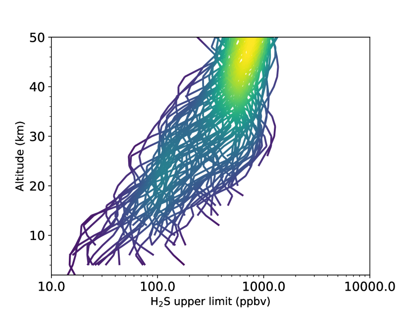
Figure 7: Retrieved 1$\sigma$ upper limits of H₂S from the position 5 dataset as a function of altitude. Colours indicate the density of retrieved values at each altitude.

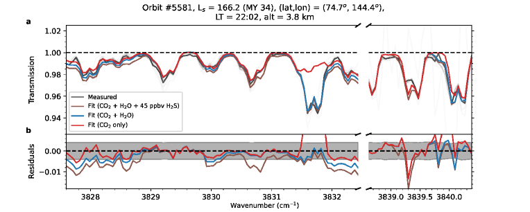
Figure 8: Upper limit of H₂S from position 5 spectra. Panel a: Fit to the spectrum with the lowest retrieved H₂S upper limit in the position 5 dataset, with a 3$\sigma$ value equivalent to 45 ppbv. In grey are the observed spectra at each row of the detector array normalised to the retrieved unity baseline (black, dashed): the darker the grey colour, the greater the weighting used for the calculation of $\mu^{*}$ and $\varsigma^{*}$. The red and blue lines respectively show the contributions of each of the interfering gas species (in this case, CO₂ and H₂O) to the fit to the row of the detector array with the greatest S/N, while the brown line shows the synthetic spectrum following the addition of 3$\sigma$ of H₂S. Panel b: Residuals of each of the gas contributions compared with the observed spectrum with the greatest S/N, where the shaded grey region represents the estimated noise level.

4.3 OCS

Although predicted outgassing of OCS is much lower than for SO₂ and H₂S, with the OCS/SO₂ ratio from terrestrial volcanic emission observed to be of the order of 10^-4 - 10^-2 (e.g. Sawyer et al., 2008; Oppenheimer & Kyle, 2008), it could nonetheless be produced indirectly from volcanic SO₂ in the high atmosphere through reaction with carbon monoxide (Hong & Fegley, 1997). Older systematic searches for OCS from Mariner 9 data (Maguire, 1977) and ground-based millimetre observations (Encrenaz et al., 1991) established upper limits in the Martian atmosphere of 70 ppbv. More recently, Khayat et al. (2017) stated upper limits of 1.1 ppbv from ground-based observations of a mid-infrared band centred at 2925 cm^-1, which was partially obscured by telluric absorption. This band is also the strongest of two OCS absorption bands that is covered by ACS MIR, specifically by grating position 11 (the other, centred around 3460 - 3500 cm^-1 and covered by grating position 3, is weaker and contaminated by strong CO₂ absorption). It also has by far the best spatial and temporal coverage out of all the three grating positions shown here, providing almost continuous coverage from the start of the ACS science phase in April 2018 (MY 34, L_s = 163°) to January 2021 (MY 35, L_s = 355°). Unlike with SO₂ and H₂S there is a relative lack of other gases that absorb in this region and would further complicate the retrieval of OCS, with the exception of HCl, which is present only during certain seasons and which is easily isolated from the OCS absorption lines. On the flip side, the lack of gases that absorb in this region can also make it difficult to fit the instrument line shape associated with spectral doubling, especially for occultations where there is an absence of HCl. This can also occasionally result in overfitting of OCS to local noise features present in the spectrum, resulting in spurious detections usually of the order of 2$\sigma$. We show this in figure 9, where the retrieved ratios of $\mu^{*}/\varsigma^{*}$ for all position 11 measurement sequences and altitudes should statistically approximate a Gaussian distribution centred around $\mu^{*}/\varsigma^{*}\approx 0$ and with a standard deviation equivalent to $\mu^{*}/\varsigma^{*}$, but we instead find some positive kurtosis due to the presence of false 2$\sigma$ detections. Nonetheless, the effect of overfitting noise is somewhat mitigated through averaging over adjacent rows on the detector array, and we find no evidence of OCS in our observations above a 3$\sigma$ confidence level.

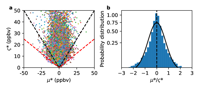
Figure 9: Statistical distribution of the retrieved values of $\mu^{*}$ and $\varsigma^{*}$ for OCS from all position 11 spectra in the analysed dataset. Panel a: Scatter plot of $\mu^{*}$ against $\varsigma^{*}$, with the dashed black line showing the 1$\sigma$ detection threshold and the dashed red line showing the 2$\sigma$ detection threshold. Panel b: Normalised probability distribution of derived $\sigma$ detection values, with the solid black line showing the Gaussian best fit to the probability distribution. While we find little skew in our upper limit retrievals, there is some kurtosis due to occasional overfitting of fixed pattern noise.

As with SO₂, the greatest density of retrieved upper limits can be found around 20 km of altitude as shown in Fig. 10, where values of 2-3 ppbv can regularly be sought even in regions of high dust concentration. Unlike with SO₂, however, observations at lower altitudes are much less limited by the presence of systematic uncertainties or aerosols, which allows for smaller upper limit values to be sought much closer to the surface. In Fig. 11 we show that the lowest upper limits can be obtained at the winter poles down to 0.4 ppbv, where the atmosphere can be probed by ACS MIR down to around 2 km above the areoid, and especially the southern hemisphere during winter solstice where global or regional dust activity is minimal, for which the best example is shown in Fig. 12. By contrast, the perihelion dust season usually limits detections to above 1 ppbv, in line with previous upper limit estimates from Khayat et al. (2017) that were obtained through co-adding of both aphelion and perihelion observations. This is also an improvement on theoretical upper limit estimates previously predicted for ACS MIR by Korablev et al. (2018), where the expected performance of the instrument only predicted values down to 2 ppbv even in clear atmospheric conditions. Nonetheless, if we were to attempt to search for real OCS outgassing given an upper limit constraint of 20 ppbv provided by our SO₂ retrievals, together with the constraints on the OCS/SO₂ provided by terrestrial volcanoes, even if we were to assume a very high ratio of OCS/SO₂= 10^-2 we would realistically require sensitivity to OCS below at least 0.2 ppbv. This is also complicated by the fact that OCS is difficult to form at low temperatures according to the Hong & Fegley (1997) reaction mechanism and would require very hot sub-surface temperatures to be present on Mars. Oppenheimer et al. (2011) quote OCS/SO₂ ratios for the Antarctic volcano Erebus of $7\times 10^{-3}$, equivalent to a maximum of 0.15 ppbv of OCS given detected SO₂ values on Mars. All these criteria make it very unlikely that ACS MIR would be able to find OCS in the Martian atmosphere in sufficiently high quantities to be detected.

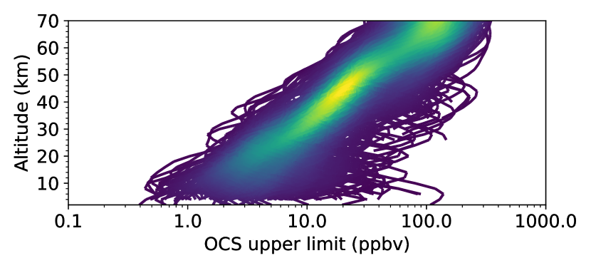
Figure 10: Retrieved 1$\sigma$ upper limit values of OCS from all position 11 measurement sequences analysed in the dataset. Colours indicate the density of upper limit values as in Figs. 4 and 7.

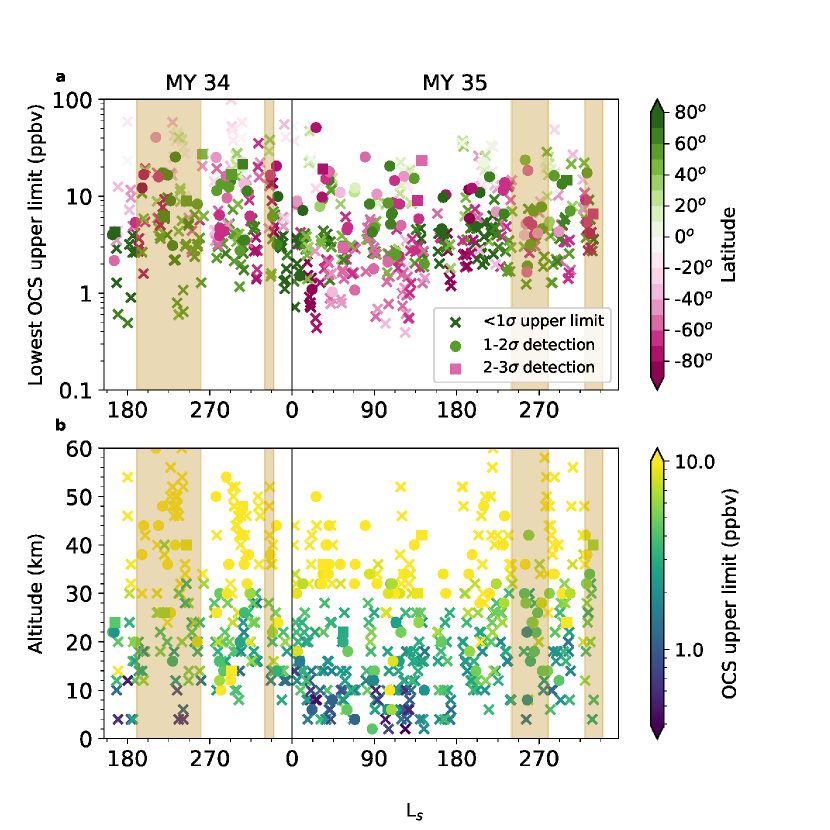
Figure 11: Seasonal distribution of lowest OCS upper limit values from each position 11 measurement sequence, as a function of latitude (Panel a) and altitude (Panel b). Crosses denote upper limits of below 1$\sigma$ significance, circles denote detections of between 1$\sigma$ and 2$\sigma$, and squares denote detections of between 2$\sigma$ and 3$\sigma.$ Brown shaded regions indicate major dust storm events, as in Fig. 5. No positive detections of OCS above 3$\sigma$ were found in the data.

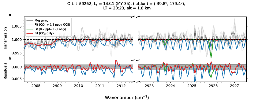
Figure 12: Upper limit of OCS from position 11 spectra. Panel a: Fit to the spectrum with the lowest retrieved OCS upper limit in the position 11 dataset, with a 3$\sigma$ value equivalent to 1.2 ppbv. As in Fig. 8, the grey lines represent each of the spectra on the detector array used to estimate the OCS detection limit, where the darker the grey colour, the higher the S/N. On the left we show the fit to the spectrum in diffraction order 173, and to the right we show the simultaneous fit to order 174. For reference, we also plot the approximate 3$\sigma$ upper limit of HCl in green, equivalent to 0.2 ppbv, as well as the contribution of CO₂ to the fit. Panel b: Residuals of the spectral fit.

5 Discussion and conclusion

In this analysis we present the results of a systematic study of multiple solar occultation observations of Mars during Martian years 34 and 35 using ACS MIR, with the aim of either detecting or establishing upper limits on the presence of three major signatures of volcanic outgassing. For SO₂, we constrain gas abundances to below 20 ppbv. Assuming that SO₂ is well mixed in the atmosphere following an eruption that happened more than six months prior, and assuming a total mass of the atmosphere of approximately $2.5\times 10^{16}$ kg, this translates to a total maximum limit of approximately 750 ktons of SO₂ in the atmosphere, averaging an outgassing rate of less than 2 ktons a day if we assume that SO₂ has a lifetime in the Martian atmosphere of approximately 2 years. For comparison, the most active volcanoes on Earth – Etna in Sicily and Kilauea in Hawaii – have passive outgassing rates of SO₂ of approximately 5.5 ktons/day and 0.98 ktons/day, respectively (Oppenheimer et al. 2011; and references therein), while a single eruption of a Volcanic Explosivity Index (VEI) of 3, equivalent to a small eruption that is expected to occur approximately once every few months on Earth, can be expected to emit around 700 ktons of SO₂ into the atmosphere (Graf et al., 1997). This appears to reinforce the prevailing view that residual present-day volcanic activity on Mars can only exist at an extremely low level, if at all. In addition, we derive H₂S upper limits down to 16 ppbv and OCS upper limits down to 0.4 ppbv in the best cases, the latter value being lower than any values previously published. However, these are unlikely to be of sufficient sensitivity for ACS MIR to detect passive outgassing from the surface of Mars. For all three molecules, no positive detections beyond 3$\sigma$ were found to be present in the ACS MIR data.

The lack of sulphur compounds detected in the Martian atmosphere has implications for the origin of two other molecules that have been detected in recent years. Halogen halides (HF, HCl, HBr, and HI) are known to be emitted by terrestrial volcanoes, and only one, HCl, has so far been confirmed to exist in the Martian atmosphere. HCl was seen to peak in abundances of the order of a few ppbv in the second half of both MY 34 and MY35, between the global and regional dust storm periods (Korablev et al., 2021; Olsen et al., 2021c). The HCl/SO₂ mass ratio in gases emitted from terrestrial volcanoes is variable but usually lies between around 0.1 - 0.9 (Pyle & Mather, 2009). This would be just compatible with the SO₂ upper limits found in this work, although seasonal trends in HCl concentration appear not to favour a primarily volcanic origin. With regards to the origin of methane, the ratio of CH₄/SO₂ emitted by terrestrial volcanoes is 1.53 at the most, and usually much smaller (Nakagawa et al. 2009; and references therein). The recent 20 ppbv and 45 ppbv methane spikes claimed by Moores et al. (2019) and Mumma et al. (2009) would therefore only be partially justifiable as being of volcanic origin, assuming they are confirmed to be genuine.

ACS MIR observations of SO₂ and H₂S have so far been hampered by a lack of spatial and temporal coverage, as well as an instrument line shape function that as yet remains incompletely characterised. Additional measurements in the future could allow us to probe deeper into the atmosphere and drive down upper limits on SO₂ and H₂S even further to definitively constrain the amount of outgassing from the surface of Mars, especially around regions near the tropics such as Cerberus Fossae, where signs of intermittent volcanism are the most promising.

Appendix A Detailed procedure of upper limit derivation for H₂S and OCS

We assume that in the case where the trace gas cannot be identified from the spectra, the volume mixing ratio of the trace gas measured at each altitude follows a Gaussian distribution centred at a zero abundance value, with a standard deviation corresponding to the uncertainty in the retrieved profile due to both spectral noise and sources of systematic error as per Montmessin et al. (2021) and Knutsen et al. (2021). This means that we want to ensure that there is as little prior constraint on the vertical profile as possible, and ensure that vertical correlations are sufficiently small to induce oscillations in the retrieved profiles that approximately reflect the sigma uncertainty level at each altitude. The six-step procedure is summarised as follows.

Step 1: We estimated the S/N from random noise by measuring the degree of fluctuation around local maxima present in each transmission spectrum (method 3 in Braude et al. 2021).

Step 2: We performed a preliminary retrieval of the trace species abundance in question, together with any other instrumental and atmospheric parameters, allowing as much variability as possible.

Step 3: In order to estimate the contribution of spectral uncertainty from sources of systematic error that are difficult to quantify (such as forward modelling error or local calibration artefacts), we divided the S/N estimated in step 1 at each tangent height by the square root of the reduced $\chi^{2}$ value obtained at each tangent height, analogously to Montmessin et al. (2021).

Step 4: In order to further reduce biases from the prior and errors in convergence due to ill conditioning, we performed a final retrieval with the prior trace gas profile being the retrieved profile from step 3 multiplied by -1, and with the prior errors on the trace gas profile reduced by an order of magnitude. This also allows a detection to be more easily distinguished from a non-detection.

Step 5: We repeated steps 1 - 4 for approximately seven rows on the detector array for a given diffraction order, with the rows chosen to sample the change in the S/N over the detector array.

Step 6: The detection limit at each altitude, $j$, was then the weighted mean, $\mu_{j}^{*}$, plus the weighted standard deviation, $\varsigma_{j}^{*}$, of the trace gas abundance values, $x_{ijk}$, retrieved from each row, i, of the detector array, with $k=1$ corresponding to the value retrieved from step 3 and $k=2$ corresponding to that retrieved from step 4 (with a posteriori variance $\Delta_{ijk}$ on the value of $x_{ijk}$ determined through propagation of errors in each retrieval):

$$\mu_{j}^{*}=\frac{\sum_{k=1}^{2}\sum_{i=1}^{N}\frac{x_{ijk}}{\Delta_{ijk}}}{\sum_{k=1}^{2}\sum_{i=1}^{N}\frac{1}{\Delta_{ijk}}}$$ (4)

$$\varsigma_{j}^{*}=\sqrt{\frac{\sum_{k=1}^{2}\sum_{i=1}^{N}\frac{(x_{ijk}-\mu_{j}^{*})^{2}}{\Delta_{ijk}}}{\left(\sum_{k=1}^{2}\sum_{i=1}^{N}\frac{1}{\Delta_{ijk}}\right)-\frac{\left(\sum_{k=1}^{2}\sum_{i=1}^{N}\frac{1}{\Delta_{ijk}}^{2}\right)}{\left(\sum_{k=1}^{2}\sum_{i=1}^{N}\frac{1}{\Delta_{ijk}}\right)}}},$$ (5)

where N is the number of detector rows sampled in the diffraction order. The weighting factor $\frac{1}{\Delta_{ijk}}$implicitly takes into account the fact that the noise profile, S/N and the quality of the spectral fit vary from row to row, and acts to maximise the contribution of rows where the fit is optimal and noise is reduced. Hence the parameter $\varsigma_{j}^{*}$ can be thought of as the total uncertainty on the retrieved gas profile due to random noise, while the parameter $\mu_{j}^{*}$ represents total systematic offsets in the retrieved gas profile that are either due to genuine absorption lines or due to systematic uncertainties such as calibration artefacts or forward modelling error.