The Application of Zig-Zag Sampler in Sequential Markov Chain Monte Carlo

Abstract

Particle filtering methods are widely applied in sequential state estimation within nonlinear non-Gaussian state space model. However, the traditional particle filtering methods suffer the weight degeneracy in the high-dimensional state space model. Currently, there are many methods to improve the performance of particle filtering in high-dimensional state space model. Among these, the more advanced method is to construct the Sequential Markov chain Monte Carlo (SMCMC) framework by implementing the Composite Metropolis-Hasting (MH) Kernel. In this paper, we proposed to discretize the Zig-Zag Sampler and apply the Zig-Zag Sampler in the refinement stage of the Composite MH Kernel within the SMCMC framework which is implemented the invertible particle flow in the joint draw stage. We evaluate the performance of proposed method through numerical experiments of the challenging complex high-dimensional filtering examples. Numerical experiments show that in high-dimensional state estimation examples, the proposed method improves estimation accuracy and increases the acceptance ratio compared with state-of-the-art filtering methods.

I Introduction

Estimating signal from a series of noisy observations is an crucial assignment in many applications, especially in the weather fields and multi-target tracking [1] [2] [3]. Nonlinear non-Gaussian state space model is widely used in these applications and Sequential Monte Carlo (SMC) [4] methods are employed to deal with the inference problem of state space model. However, SMC are inefficient in the high-dimensional state sapce model because SMC use the importance sampling method as the bias correction. Importance sampling could lead to high variance of estimation result. Therefore, in the high-dimensional situation, the weight of large number of particles is almost zero and this phenomenon is called weight degeneracy. Although the variance could be minimized by using optimal importance distribution, it is difficult to sample from optimal importance distribution [4]. As a further matter, the performance of SMC also depends on the design of importance distribution which need to be designed according to different model [5]. This undoubtedly increases the difficulty of solving the filtering problem by implementing the SMC methods.

In the past few decades, several methods for improving the performance of particle filtering have been developed. The first kind of methods are auxiliary particle filtering (APF) [6], unscented particle filtering [7], and RaoBlackwellised particle filtering [8]. These methods aim to approximate the optimal importance distribution by designing proposal distribution. APF methods improve the sampling efficiency by way of introducing new auxiliary variable. Unscented particle filtering methods use the unscented transformation to approximate the optimal importance distribution. RaoBlackwellised particle filtering methods combine Kalman filter [9] and particle filtering to improve the performance. These methods can only perform well in some specific situations and state estimation in the high-dimensional situation is still a challenging mission. The second kind of methods are extended Kalman filter (EKF) [10], unscented Kalman filter (UKF) [11], and the ensemble Kalman filter (EnKF) [12]. These methods rely on local linearization medium and crude functional approximation method. EnKF and EKF can perform well with the state space model which have Gaussian error and UKF can perform well with the state space model which have non-Gaussian error. These methods also cannot be completely applied in the nonlinear non-Gaussian state space model. The third kind of methods are multiple particle filtering [13], block particle filtering [14], and space-time particle filtering [15]. Their core approach is decomposition or partition of state space and transforming a high-dimensional problem into a low-dimensional problem. But these methods cannot completely solve the problem of “dimension curse” caused by weight degeneracy.

Compared with SMC, Sequential Markov Chain Monte Carlo (SMCMC) [16] are another methods to solve the filtering problem and successfully applied within the nonlinear non-Gaussian high-dimensional state space model. The main idea of SMCMC is to construct a Markov chain which stationary distribution is empirical approximation of posterior distribution and sample particles from the transition kernel. SMCMC combines the recursive nature of SMC and the high performance of Markov Chain Monte Carlo (MCMC) methods. Besides, SMCMC uses the rejection-acception sampling mechanism as the bias correction. Therefore, the first advantage of SMCMC is that we do not care about the weight degeneracy in the SMCMC framework. The performance of SMCMC depends on the transition kernel. Thus, exploring an efficient transition kernel is an important mission. Luckily, SMCMC could use all MCMC kernel [17] which is another advantage of SMCMC. There are mainly four types of transition kernel of SMCMC in [18]: Optimal Independent Metropolis-Hasting (MH) Kernel, Approximation of the Optimal Independent MH Kernel, Independent MH Kernel Based on Prior as Proposal, and Composite MH Kernel. Optimal Independent MH Kernel is difficult to design under normal circumstances. Compared with Approximation of the Optimal Independent MH Kernel and Independent MH Kernel Based on Prior as Proposal, Composite MH Kernel performs well in the high-dimensional situation because Composite MH Kernel could gradually collect information of the target distribution, this means, Composite MH Kernel could explore the neighborhood of the current value of Markov chain [18].

Although Composite MH Kernel is more efficient than other SMCMC kernels, there are some methods to further improve the performance of Composite MH Kernel. The Metropolis Adjusted Langevin Algorithm (MALA) [19] [20] [21] and Hamiltonian Monte Carlo (HMC) [22] which based on Riemannian manifold are proposed as the refinement step in the Composite MH kernel. After combining with Composite MH Kernel, MALA and HMC can have better performance in the high-dimensional state space model. Reference [18] showed that the sequential manifold HMC (SmHMC) method performs better than sequential MALA (SMALA) method. On the other hand, the SmHMC method also has a limitation that target distribution needs to satisfy the log-concave condition. Although there are ways to solve this problem, the expected values of negative Hessian and some hyperparameters are still required.

Recently, a novel class of methods called invertible particle flow [23] is proposed to implement and construct the first proposal distribution in the Composite MH Kernel. Invertible particle flow can guide particles from prior to posterior distribution, that means it could approximate the true posterior density from the handleable prior density through the intermediate density. Therefore, invertible particle flow can be used to construct a proposal distribution which closes to the posterior distribution in the join draw step of Composite MH Kernel. There are two advantages of implementing invertible particle flow in the Composite MH Kernel. This combination could better close the Optimal Independent MH Kernel and improve the sampling efficient in the joint draw step. Exact Daum-Huang (EDH) method and local Exact Daum-Huang (LEDH) [24] method are one of the invertible particle flow methods and further improves the performance of Composite MH Kernel.

In recently past, research in non-reversible piecewise deterministic MCMC (PD-MCMC) [25] [26] field has made great progress. The key idea of PD-MCMC is to use the non-reversible piecewise deterministic Markov process (PDMP) [27] [28] to sample from the target distribution which as its invariant distribution. On one hand, non-reversible PDMP have better mix properties compared to reversible Markov process. Thus, PD-MCMC could yield estimation values with low variance. On the other hand, PD-MCMC methods are rejection-free methods, this means, every data sampled would not be dropped. Therefore, it could explore the target distribution more efficiently, especially in the case of high-dimensional and Big-Data. Classical examples of PDMP are Bouncy Particle Sampler (BPS) [29] and Zig-Zag Sampler [30].

Even though there are many advantages of PD-MCMC, it cannot be directly used in the SMCMC framework. First, if we want to construct the PDMP, we need to simulate the inhomogeneous Poisson process. In complicated situation, inhomogeneous Poisson process is simulated by the Poisson thinning method. Thus, it requires to know the local upper bound of the derivative of the log posterior distribution. However, local upper bound is difficult to obtain. Second, the PDMP methods mentioned above are all based on continuous conditions. However, discrete condition need to be satisfied in the SMCMC framework. Therefore, Discrete Bouncy Particle Sampler (DBPS) is proposed in [29]. DBPS is discrete version of BPS and can be implemented without simulating inhomogeneous Poisson process. Reference [31] proposed that implementing DBPS as refinement step in the Composite MH Kernel of SMCMC framework and DBPS could further improve the acceptance ratio compared with other MCMC methods. But like BPS, DBPS still has a phenomenon called reducible. Adding the velocity refresh step in the DBPS can solve reducible problem. Reference [29] proposes three speed refresh methods: Full refresh, Ornstein-Uhlenbeck refresh, and Brownian motion on the unit sphere refresh. However, there is no general method to determine the velocity refresh. We need to choose different velocity method that is suitable for the situation. Moreover, improper velocity refresh method will greatly reduce the efficiency of the DBPS [32].

In this paper, we propose to discretize the Zig-Zag Sampler and combine it with the SMCMC framework as the individual refinement step. In addition, we still employ the EDH method to construct the first proposal distribution in the Composite MH Kernel of SMCMC framework. Compared with the advanced methods in this field, our main contributions include: 1) we exploit the mild ergodic condition of Zig-Zag Sampler to avoid choosing suitable velocity refresh method in the SMCMC framework; 2) we employ the better mix properties of Zig-Zag Sampler which can provide higher particle diversity and improve the acceptance ratio comparing with traditional SmHMC and MALA methods in the SMCMC framework; 3) we exhibit the effiency of the proposed method in the complex inference scheme with the high-dimensional state space model.

We organize the rest of the paper as below. In Section II, we perform the problem statement. In Section III, we present a brief review of SMCMC, Composite MH Kernel, EDH, and LEDH. In Section IV, we describe the proposed method which combining discretized Zig-Zag Sampler and EDH in the SMCMC framework. In Section V, we describe the numerical experiments and exhibit the results. In Section VI, we outline the contributions and results.

II Problem Statement

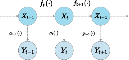
Figure 1: Graphical representation of state space model.

In the nonlinear non-Gaussian state space model inference problem, we interested in obtaining the marginal posterior probability density $p(x_{t}|y_{1:t})$. $x_{t}$ is the state of the dynamic system at time $t$ and $y_{1:t}=\{y_{1},...,y_{t}\}$ is a sequence collection of observations up to time $t$. We can consider to model the state equation and observation equation by the following state sapce model:

$$x_{0} \sim\mu_{0}(x)$$ (1)

$$x_{t} =f_{t}\left(x_{t-1},v_{t}\right)\quad\text{ for }t\geq 1,$$ (2)

$$y_{t} =g_{t}\left(x_{t},w_{t}\right)\quad\quad\text{ for }t\geq 1.$$ (3)

Here $\mu_{0}(x)$ is the initial probability density function of the initial state $x_{0}$ which means the time step before any observations arrives. The function $f_{t}:\mathbb{R}^{d}\times\mathbb{R}^{d^{\prime}}\rightarrow\mathbb{R}^{d}$ is the state equation which describes the dynamic of the unknown state $x_{t}\in\mathbb{R}^{d}$ and the system noise $v_{t}\in\mathbb{R}^{d^{\prime}}$. Observation $y_{t}$ is generated by the $g_{t}:\mathbb{R}^{d}\times\mathbb{R}^{C^{\prime}}\rightarrow\mathbb{R}^{C}$ which is the observation equation and describes the relationship between observation $y_{t}$, state $x_{t}$, and the observation noise $w_{t}\in\mathbb{R}^{d^{\prime}}$. We assume that $f_{t}(\cdot,0)$ is bounded, and $g_{t}(\cdot,0)$ is a $C_{1}$ function, i.e.,$g_{t}(\cdot,0)$ is differentiable everywhere and its derivatives are continuous.

III Background Material

III-A Sequential Markov Chain Monte Carlo Methods

SMCMC methods are proposed as efficient tool to solve the state estimation task of high-dimensional state space model. The key idea of SMCMC methods is to implement the MH accept-reject way and use the proposal distribution by which current states are sampled. Then, after obtaining samples, the target distribution is approximated by them. At time step $t$, we interested in sampling state from the target distribution:

$$\pi_{t}\left(x_{1:t}\right) =p\left(x_{1:t}\mid y_{1:t}\right)$$

$$=p\left(x_{1:t-1}\mid y_{1:t-1}\right)\frac{p\left(x_{t}\mid x_{t-1}\right)p\left(y_{t}\mid x_{t}\right)}{p\left(y_{t}\mid y_{1:t-1}\right)}$$

$$\propto p\left(x_{t}\mid x_{t-1}\right)p\left(y_{t}\mid x_{t}\right)p\left(x_{1:t-1}\mid y_{1:t-1}\right)$$

$$\propto p\left(x_{t}\mid x_{t-1}\right)p\left(y_{t}\mid x_{t}\right)\pi_{t-1}\left(x_{1:t-1}\right)$$ (4)

Unfortunately, it is very difficult to sample from the $\pi_{t-1}\left(x_{1:t-1}\right)$ which is analytically intractable in the general nonlinear non-Gaussian state space model. Therefore, the empirical approximation distribution is proposed to replace $\pi_{t-1}\left(x_{1:t-1}\right)$. The empirical approximation distribution could be obtained after the previous recursion and defined as:

$$\widehat{\pi}_{t-1}\left(dx_{1:t-1}\right)=\frac{1}{N}\sum_{m=N_{b}+1}^{N+N_{b}}\delta_{X_{t-1,1:t-1}^{m}}\left(dx_{1:t-1}\right)$$ (5)

then we replace the distribution of interest with the following equation (6) [18]:

$$\breve{\pi}_{t}\left(x_{1:t}\right)\propto p\left(y_{t}\mid x_{t}\right)p\left(x_{t}\mid x_{t-1}\right)\widehat{\pi}_{t-1}\left(x_{1:t-1}\right)$$ (6)

Here $N_{b}$ is the number of burn-in samples and $N$ is the number of reserved samples, $\delta$ is the Dirac delta function. $\left\{X_{t-1,1:t-1}^{m}\right\}_{m=N_{b}+1}^{N_{b}+N}$ are the $N$ samples obtained from the Markov chain at time $t-1$, whose stationary distribution is $\breve{\pi}_{t-1}\left(x_{1:{t-1}}\right)$ and $\mathcal{K}_{t}$ is an MCMC kernel of invariant distribution $\breve{\pi}_{t}\left(x_{1:t}\right)$. Finally, at the time $t$, we obtain the approximation of marginal posterior distribution by the following equation:

$$p\left(x_{t}\mid y_{1:t}\right)\approx\frac{1}{N}\sum_{m=N_{b}+1}^{N+N_{b}}\delta_{X^{m}_{t,1:t}}\left(dx_{t}\right)$$ (7)

In Algorithm 1 [18], we summarized the general framework of the SMCMC.

Algorithm 1 Generic SMCMC framework

1:if time $t=1$ then

2:     for $j=1,...,N+N_{b}$ do

3:         Sample $X_{1,1}^{j}\sim\mathcal{K}_{1}(X^{j-1}_{1,1},\cdot)$ with $\mathcal{K}_{1}$ an MCMC kernel of invariant distribution $\pi_{1}(x_{1})\propto g_{1}(y_{1}\mid x_{1})\mu(x_{1})$

4:     end for

5:else if time $t\geq 2$ then

6:     for $j=1,...,N+N_{b}$ do

7:         Refine empirical approximation of previous posterior distribution.

8:         Sample $X_{t,1:t}^{j}\sim\mathcal{K}_{t}(X^{j-1}_{t,1:t},\cdot)$ with $\mathcal{K}_{1}$ an MCMC kernel of invariant distribution $\breve{\pi}_{t}\left(x_{1:t}\right)$ defined in (6)

9:     end for

10:end if

11:Approximation of the smoothing distribution with the following empirical measure:

$$\pi\left(x_{1:t}\right)\approx\frac{1}{N}\sum_{j=N_{b}+1}^{N+N_{b}}\delta_{X_{t,1:t}^{j}}\left(dx_{1:t}\right)$$

III-B Composite MH Kernel

The performance of SMCMC is heavily dependent on MCMC kernel. A properly designed transition kernel can greatly improve the performance of SMCMC in the high-dimensional situation. Some different SMCMC kernels are introduced in [18] [33]. The optimal choice of transition kernel is the Optimal Independent MH Kernel in which the proposal distribution is independent of the current value. However, the proposal distribution is constructed by the target distribution in the framework of Optimal Independent MH Kernel. Therefore, it is difficult to adopt this scheme in most cases.

Subsequently, Approximation of the Optimal Independent MH Kernel and Independent MH Kernel Based on Prior as Proposal are proposed to approximate the Optimal Independent MH Kernel by using Laplace approximation or local linearization techniques. But it cannot be easy to approximate accurately and acceptance ratio could be very little in the complex or high-dimensional situation.

Composite MH Kernel uses local proposal instead of global proposal, so it will reduce the dependence on the target distribution, and thus be more efficient. The Composite MH Kernel method is summarized in Algorithm 2.

Algorithm 2 Composite MH Kernel in a unifying framework of SMCMC [18]

1:$x^{j-1}_{t,0:t}$

2:$x^{j}_{t,0:t}$

3:$Joint~{}Draw$

4:Propose $x_{t,0:t}^{*}\sim q_{t,1}(x_{0:t}\mid x_{t,0:t}^{j-1})$;

5:Compute the MH acceptance ratio

6:$\rho_{1}=\min(1,\frac{\breve{\pi}_{t}(x_{t,0:t}^{*})}{q_{t,1}(x_{t,0:t}^{*}\mid x_{t,0:t}^{j-1})}\frac{q_{t,1}(x_{t,0:t}^{j-1}\mid x_{t,0:t}^{*})}{\breve{\pi}_{t}(x_{t,0:t}^{j-1})})$;

7:Accept $x_{t,0:t}^{j}=x^{*}_{t,0:t}$ with probability $\rho_{1}$, otherwise set $x_{t,0:t}^{j}=x^{j-1}_{t,0:t}$;

8:$Individuate~{}refinement~{}of~{}x_{t,0:t-1}^{j}$;

9:Propose $x_{t,0:t-1}^{*}\sim q_{t,2}(x_{0:t-1}\mid x_{t,0:t}^{j})$;

10:Compute the MH acceptance ratio

11:$\rho_{2}=\min(1,\frac{\breve{\pi}_{t}(x_{t,0:t-1}^{*},x_{t,t}^{j})}{q_{t,2}(x_{t,0:t-1}^{*}\mid x_{t,0:t}^{j})}\frac{q_{t,2}(x_{t,0:t-1}^{j}\mid x_{t,0:t-1}^{*},x_{t,t}^{j})}{\breve{\pi}_{t}(x_{t,0:t}^{j})})$;

12:Accept $x_{t,0:t-1}^{j}=x^{*}_{t,0:t-1}$ with probability $\rho_{2}$, otherwise set $x_{t,0:t-1}^{j}=x^{j-1}_{t,0:t-1}$;

13:$Individual~{}refinement~{}of~{}x^{j}_{t,t}$

14:Propose $x_{t,t}^{*}\sim q_{t,3}(x_{t}\mid x_{t,0:t}^{j})$

15:Compute the MH acceptance ratio

16:$\rho_{3}=\min(1,\frac{\breve{\pi}_{t}(x_{t,0:t-1}^{j},x_{t,t}^{*})}{q_{t,3}(x_{t,t}^{*}\mid x_{t,0:t}^{j})}\frac{q_{t,3}(x_{t,t}^{j}\mid x_{t,0:t-1}^{j},x_{t,t}^{*})}{\breve{\pi}_{t}(x_{t,0:t}^{j})})$;

17:Accept $x_{t,t}^{j}=x^{*}_{t,t}$ with probability $\rho_{3}$, otherwise set $x_{t,t}^{j}=x^{j-1}_{t,t}$;

Reference [18] proposed to use Composite MH Kernel which composed of joint draw step and refinement step. It performs more efficient in the high-dimensional situation. Here, $q_{t,1}(\cdot)$ is the first proposal distribution, $q_{t,2}(\cdot)$ is the second proposal distribution, and $q_{t,3}(\cdot)$ is the third proposal distribution. All path of states are updated by using MH sampler in the joint draw step. In the refinement step, previous obtained $x_{1:t-1}$ and current $x_{t}$ are updated in order. In addition, any MCMC kernel could be employed in the Composite MH Kernel. Therefore, Independent MH Kernel Based on Prior as Proposal usually is implemented in the joint draw step as the first proposal distribution and $\widehat{\pi}_{t-1}$ is implemented in the individual refinement step as the second proposal distribution $q_{t,2}(\cdot)$. However, the block MH-within Gibbs sampling is employed as the refinement step in the traditional Composite MH Kernel and it will result in extremely low sampling rate. In order to improve the efficient, HMC and DBPS [31] is proposed as the refinement step to construct $q_{t,3}(\cdot)$ in the Composite MH Kernel and these methods are become one class of the most effective methods.

III-C Invertible Particle Flow

Recently, a new class of Monte Carlo-based filtering called invertible particle flow [34] is proposed and perform well in the high-dimensional state space model. Assume that $N$ particles $\{x^{j}_{t-1}\}^{N}_{j=1}$ are obtained at time step $t-1$. $\{x^{j}_{t-1}\}^{N}_{j=1}$ are employed to approximate the target distribution. After implanting by the state equation at time $t$, we obtain $\{\tilde{x}_{t}^{j}\}_{j=1}^{N}$ which means the predictive target distribution at time step $t$. Then, particle flow could migrate the particles and lead the particles approximate the posterior distribution well.

Invertible particle flow could be implemented as a background stochastic process $\eta_{\lambda}$ in a pseudo time interval $\lambda\in[0,1]$. Under normal circumstances, we assume that $\{\tilde{x}_{t}^{j}\}_{j=1}^{N}$ is replaced by $\{\eta_{0}^{j}\}_{j=1}^{N}$. After the whole dynamic stochastic process is completed, we obtain $\{\eta_{1}^{j}\}_{j=1}^{N}$ which is regarded as the particles that approximate the target distribution.

In [35] [36], the invertible particle flow $\{\eta_{0}^{j}\}_{j=1}^{N}$, follows equation (8):

$$\frac{d\eta_{\lambda}^{j}}{d\lambda}=\zeta(\eta_{\lambda}^{j},\lambda)$$ (8)

where $\zeta$ is constrained by the Fokker-Planck equation with zero diffusion:

$$\frac{\partial p(\eta_{\lambda}^{j},\lambda)}{\partial\lambda}= -p(\eta_{\lambda}^{j},\lambda)\operatorname{div}(\zeta(\eta_{\lambda}^{j},\lambda))$$

$$-\frac{\partial p(\eta_{\lambda}^{j},\lambda)}{\partial\eta_{\lambda}^{j}}\zeta(\eta_{\lambda}^{j},\lambda)$$ (9)

where $p$ is the probability density of $\eta_{\lambda}$. In this paper, we mainly introduced two invertible particle flow methods: Exact Daum and Huang Filter (EDH) method and local Exact Daum and Huang Filter (LEDH) method.

III-C1 The Exact Daum and Huang Filter with SMCMC

The particles flow trajectory of $\eta_{\lambda}$ in the exact Daum and Huang Filter [37] [38] follows this equation:

$$\zeta(\eta_{\lambda}^{j},\lambda)=A(\lambda)\eta_{\lambda}^{j}+b(\lambda)$$ (10)

Here, $A(\lambda)$ and $b(\lambda)$ is presented in [39]:

$$A(\lambda) =-\frac{1}{2}PH(\lambda)^{T}\left(\lambda H(\lambda)PH(\lambda)^{T}+R\right)^{-1}H(\lambda)$$

$$b(\lambda) =(I+2\lambda A(\lambda))\left[(I+\lambda A(\lambda))PH(\lambda)^{T}R^{-1}q(\lambda)\right]$$

$$q(\lambda) =(y-e(\lambda))+A(\lambda)\bar{\eta}_{0}$$

$$e(\lambda) =h\left(\bar{\eta}_{\lambda},0\right)-H(\lambda)\bar{\eta}_{\lambda}$$

Here $P$ is the covariance matrix of system noise error in the state equation, $y$ is still the observation, $H$ is the observation matrix and $R$ is the covariance matrix of the observation noise. For nonlinear observation equation, $H$ requires to be constructed by the linearization technique which is employed at the mean of particles $\eta_{\lambda}$ and following the equation (11):

$$H(\lambda)=\left.\frac{\partial h(\eta,0)}{\partial\eta}\right|_{\eta=\bar{\eta}_{\lambda}}$$ (11)

Numerical integration is employed to approximate the solution of equation (8) when implementing the exact flow algorithm. Assume that we obtain a set which includes the different time step point. These time step point are $\lambda_{0},\lambda_{1},..,\lambda_{N_{\lambda}}$ and they satisfy the condition which is $0=\lambda_{0}<\lambda_{1}<\ldots<\lambda_{N_{\lambda}}=1$. The time interval $\varepsilon_{m}=\lambda_{m}-\lambda_{m-1}$ and the sum of total time interval is $1$, i.g., $\sum_{i=1}^{N_{\lambda}}\varepsilon_{i}=1$. Therefore, the integral between two adjacent of EDH follows this equation:

$$\eta_{\lambda_{m}}^{j} =f_{\lambda_{m}}(\eta_{\lambda_{m-1}}^{j})$$

$$=\eta_{\lambda_{m-1}}^{j}+\epsilon_{m}(A(\lambda_{m})\eta_{\lambda_{m-1}}^{j}+b(\lambda_{m}))$$

Thus, by using the Euler update rule [40],

$$\begin{split}\eta_{1}^{j}&=f_{\lambda_{N_{\lambda}}}\left(f_{\lambda_{N-1}}\left(\ldots f_{\lambda_{1}}\left(\eta_{0}^{j}\right)\right)\right.\\ &=\left(I+\epsilon_{N_{\lambda}}A\left(\lambda_{N_{\lambda}}\right)\right)\eta_{\lambda_{N_{\lambda}-1}}^{j}+\epsilon_{N_{\lambda}}b\left(\lambda_{N_{\lambda}}\right)\\ &=C\eta_{0}^{j}+D\end{split}$$ (12)

where,

$$C =\prod_{m=1}^{N_{\lambda}}\left(I+\epsilon_{N_{\lambda}+1-m}A\left(\lambda_{N_{\lambda}+1-m}\right)\right)$$

$$D =\epsilon_{N_{\lambda}}b(\lambda_{N_{\lambda}})$$

$$+\sum_{l=1}^{N_{\lambda}-1}([\prod_{m=1}^{N_{\lambda}-l}(I+\epsilon_{N_{\lambda}+1-m}A(\lambda_{N_{\lambda}+1-m}))]\epsilon_{m}b(\lambda_{m}))$$

Reference [40] proposes to employ invertible particle flow methods to construct the first proposal distribution in the Composite MH Kernel and gave two conclusions: 1) the mapping involving $\eta_{0}^{i}$ and $\eta_{1}^{i}$ is invertible mapping; 2) $C$ is invertible and the determinant of $C$ is not zero. Thus, the first proposal distribution $q_{t,1}(\cdot)$ could be constructed by invertible particle flow mapping and follows equation (13):

$$q(\eta_{1}^{j}\mid x_{t-1}^{j},z_{t})=\frac{p(\eta_{0}^{j}\mid x_{t-1}^{j})}{|\operatorname{det}(C)|}$$ (13)

The algorithm of applying EDH in Composite MH Kernel is summarized in Algorithm 4. In the Algorithm 4, we do not need to update $C$ and $D$ at every iteration and we only need to calculate once before every time step iteration. We draw the particles from the empirical distribution which is obtained from the previous time iteration. Then, after calculating the mean of particles, we calculate the auxiliary state $\overline{\eta}_{0}$ and employ the $\overline{\eta}_{0}$ in the $T$ function. Finally, we obtain the parameters $C$, $D$ and apply them in the SMCMC iterations with every particle at current time. About $T$ function, it is summarized in the Algorithm 3. For applying EDH to construct the first proposal distribution in the Composite MH Kernel, the first acceptance ratio is calculated by equation (14):

$$\rho_{1}=\min(1,\frac{p(x_{t,t}^{*(j)}\mid x_{t,t-1}^{*(j)})p(z_{t}\mid x_{t,t}^{*(j)})p(\eta_{0}^{j-1}\mid x_{t,t-1}^{j-1})}{p(\eta_{0}^{*(j)}\mid x_{t,t-1}^{*(j)})p(x_{t,t}^{j-1}\mid x_{t,t-1}^{j-1})p(z_{t}\mid x_{t,t}^{j-1})})$$ (14)

Algorithm 3 $T$ Function: $T(\overline{\eta})=(C,D)$

1:$\overline{\eta}$

2:$C~{}D$

3:Initialize $C=I,D=0$

4:for $m=1,...,N_{\lambda}$ do

5:     Set $\lambda_{m}=\lambda_{m-1}+\varepsilon_{m}$;

6:     Caculation $A(\lambda_{m})b(\lambda_{m})$

7:     Migrate: $\overline{\eta}:\overline{\eta}=\overline{\eta}+\varepsilon_{m}(A(\lambda_{m})\overline{\eta}+b(\lambda_{m}))$

8:     Set $C=(I+\varepsilon_{m}A(\lambda_{m}))C$;

9:     Set $D=(I+\varepsilon_{m}A(\lambda_{m}))D+\varepsilon_{j}(\lambda_{m})$;

10:end for

Algorithm 4 Composite MH Kernel with the EDH Particle Flow [40]

1:$x_{t,0:t}^{j-1},\eta^{j-1}_{0},C,D$

2:$x_{t,0:t}^{j},\eta^{j}_{0}$

3:$Joint~{}Draw~{}of~{}x_{t,0:t}^{j}$

4:Draw $x_{t,0:t-1}^{*(j)}\sim\widehat{\pi}_{t-1}\left(x_{0:t-1}\right)$

5:Sample $\eta_{0}^{*(j)}=g_{t}(x_{t,t-1}^{*(j)},v_{t})$

6:Calculate $x_{t,t}^{*(j)}=C\eta_{0}^{*(j)}+D$

7:Compute the first MH acceptance ratio $\rho_{1}=$

$$\min(1,\frac{p(x_{t,t}^{*(j)}\mid x_{t,t-1}^{*(j)})p(z_{t}\mid x_{t,t}^{*(j)})p(\eta_{0}^{j-1}\mid x_{t,t-1}^{j-1})}{p(\eta_{0}^{*(j)}\mid x_{t,t-1}^{*(j)})p(x_{t,t}^{j-1}\mid x_{t,t-1}^{j-1})p(z_{t}\mid x_{t,t}^{j-1})})$$

8:Accept $x^{j}_{t,0:t}=x_{t,0:t-1}^{*(j)},\eta^{j}_{0}=\eta_{0}^{*(j)}$ otherwise set $x^{j}_{t,0:t}=x_{t,0:t}^{j-1},\eta^{j}_{0}=\eta_{0}^{j-1}$

9:$Individuate~{}refinement~{}of~{}x_{t,0:t-1}^{j}$;

10:Propose $x_{t,0:t-1}^{*}\sim\widehat{\pi}_{t-1}(x_{0:t-1})$;

11:Compute the second MH acceptance ratio $\rho_{2}=$

$$\min(1,\frac{\breve{\pi}_{t}(x_{t,0:t-1}^{*},x_{t,t}^{j})}{q_{t,2}(x_{t,0:t-1}^{*}\mid x_{t,0:t}^{j})}\frac{q_{t,2}(x_{t,0:t-1}^{j}\mid x_{t,0:t-1}^{*},x_{t,t}^{j})}{\breve{\pi}_{t}(x_{t,0:t}^{j})})$$

12:Accept $x_{t,0:t-1}^{j}=x^{*}_{t,0:t-1}$ with probability $\rho_{2}$, otherwise set $x_{t,0:t-1}^{j}=x^{j-1}_{t,0:t-1}$;

13:$Individual~{}refinement~{}of~{}x^{j}_{t,t}$

14:Propose $x_{t,t}^{*}\sim q_{t,3}(x_{t}\mid x_{t,0:t}^{j})$

15:Compute the third MH acceptance ratio $\rho_{3}=$

$$\min(1,\frac{\breve{\pi}_{t}(x_{t,0:t-1}^{j},x_{t,t}^{*})}{q_{t,3}(x_{t,t}^{*}\mid x_{t,0:t}^{j})}\frac{q_{t,3}(x_{t,t}^{j}\mid x_{t,0:t-1}^{j},x_{t,t}^{*})}{\breve{\pi}_{t}(x_{t,0:t}^{j})})$$

16:Accept $x_{t,t}^{j}=x^{*}_{t,t}$ with probability $\rho_{3}$, otherwise set $x_{t,t}^{j}=x^{j-1}_{t,t}$;

17:Calculate $\eta^{j}_{0}=C^{-1}(x_{t,t}^{j}-D)$;

III-C2 The Local Exact Daum and Huang Filter with SMCMC

Comparing with the EDH, the system is linearized and the drift term is updated for each individual particle in the LEDH [24]. Therefore, the trajectory of every particles follows:

$$\zeta\left(\eta_{\lambda}^{j},\lambda\right)=A^{j}(\lambda)\eta_{\lambda}^{j}+b^{j}(\lambda)$$ (15)

where

$$A^{j}(\lambda) =-\frac{1}{2}PH^{j}(\lambda)^{T}\left(\lambda H^{j}(\lambda)PH^{j}(\lambda)^{T}+R\right)^{-1}H^{j}(\lambda)$$

$$b^{j}(\lambda) =\left(I+2\lambda A^{j}(\lambda)\right)\left[\left(I+\lambda A^{j}(\lambda)\right)PH^{j}(\lambda)^{T}\right.$$

$$\left.\times R^{-1}\left(y-e^{j}(\lambda)\right)+A^{j}(\lambda)\bar{\eta}_{0}\right]$$

The integral between two adjacent of LEDH follows this equation:

$$\eta_{\lambda_{m}}^{j} =f_{\lambda_{m}}^{j}(\eta_{\lambda_{m-1}}^{j})$$

$$=\eta_{\lambda_{m-1}}^{j}+\epsilon_{m}(A^{j}(\lambda_{m})\eta_{\lambda_{m-1}}^{j}+b^{j}(\lambda_{m}))$$ (16)

The algorithm of combining LEDH with Composite MH Kernel is summarized in Algorithm 5.

IV Proposal Method

The Zig-Zag Sampler [30] [41] in the continuous time situation can be seen as a discrete set of velocity [42]. When the state space is the $d$-dimensional, from a physical point of view, the velocity $v$ follows:

$$v=\sum_{i=1}^{d}v_{i}\textbf{e}_{i}$$

Here $\{\textbf{e}_{1},\textbf{e}_{2},…,\textbf{e}_{d}\}$ is a set of orthongal base vectors in the state space of $\mathbb{R}^{d}$. From a probabilistic point of view, the Zig-Zag Sampler can be considered as constructing by $d$-distinct different event type which have their own different event rate and simulate their different Possion process independently. We denote that the event rate of type $i$ is $\lambda_{i}(\textbf{x},\textbf{v})$ and thus the general event rate formulation of the Zig-Zag Sampler is

$$\lambda(\textbf{x},\textbf{v})=\sum_{i=1}^{d}\lambda_{i}(\textbf{x},\textbf{v})$$ (17)

Therefore, after simulating the next event time in every direction by using $\lambda_{i}(\textbf{x},\textbf{v})$ in equation (18),

$$\mathbb{P}(\tau_{i}\geq t)=\exp(-\int_{0}^{t}\lambda_{i}(x(s),v)ds)$$ (18)

we pick the smallest event time $\tau_{i_{0}}$ with the direction as the next event time

$$i_{0}:=\operatorname{argmin}_{i\in\{1,\ldots,d\}}\tau_{i}$$

and flip the velocity in this direction with the probability $\lambda_{i}(\textbf{x},\textbf{v})/\lambda(\textbf{x},\textbf{v})$. We denote that the flip function is $F_{i}[v]$. It means that flipping the $i$-th dimension of $v$, and follows:

$$\left(F_{i}[v]\right)_{j}=\left\{\begin{array}[]{ll}v_{j}&\text{ if }i\neq j\\ -v_{j}&\text{ if }i=j\end{array}\right.$$

In the most case, one of the important property of Zig-Zag Sampler is that the event rate could construct the relationship with the invariant distribution $\Phi(x)$ and it satisfies the following equation (19):

$$\lambda_{i}(x)={max(0,v_{i}\partial_{i}\Phi(x))}_{+}$$ (19)

Therefore, we can use equation (19) to simulate the Possion process by target distribution in the every direction.

However, we cannot directly apply traditional Zig-Zag Sampler in the SMCMC framework because it needs satisfy the discrete condition. Thus, inspired by the Zig-Zag Sampler method and in order to be able to be applied in the SMCMC framework, we used the idea of DBPS for reference and proposed to discretize the Zig-Zag Sampler. We call it the discretized Zig-Zag Sampler (DZZ).

Comparing with the troditional Zig-Zag Sampler, in the DZZ method, when the sample is rejected, we can think the event has happend at a certain direction. Thus, we calculate the dot product with every direction, like in the Zig-Zag Sampler. Becasue we want to avoid to simulate the inhomogenous Possion process, we directly obtain these dot product values as the weight of $d$-distint directions. The greater the weight, the more likely it is that the event will occur in this direction. Based on this set of weight, we randomly sample a direction index in all directions as the direction to flip the $i$-th dimension velocity $v_{i}$ of the velocity $v$. $v_{i}$ is the component of $v$ in that direction. Thus, we can implement this idea as the DZZ to construct the transition kernel.

Algorithm 5 Composite MH Kernel with the LEDH Particle Flow [40]

1:$x_{t,0:t}^{j-1},\eta^{j-1}_{0},C^{j-1},D^{j-1}$

2:$x_{t,0:t}^{j},\eta^{j}_{0},C^{j},D^{j}$

3:$Joint~{}Draw~{}of~{}x_{t,0:t}^{j}$

4:Draw $x_{t,0:t-1}^{*(j)}\sim\widehat{\pi}_{t-1}(x_{0:t-1})$

5:Sample $\eta_{0}^{*(j)}=g_{t}(x_{t,t-1}^{*(j)},v_{t})$

6:Calculate $\overline{\eta}_{0}^{*(j)}=g_{t}(x_{t,t-1}^{*(j)},0)$

7:Perform $T$ function

$$T(\overline{\eta}_{0}^{*(j)})=(C^{*(j)},D^{*(j)})$$

8:Calculate $x_{t,t}^{*(j)}=C^{*(j)}\eta_{0}^{*(j)}+D^{*(j)}$

9:Compute the first MH acceptancce ratio $\rho_{1}=$

10:$\min(1,\frac{p(x_{t,t}^{*(j)}\mid x_{t,t-1}^{*(j)})p(z_{t}\mid x_{t,t}^{*(j)})|\operatorname{det}(C^{*(j)})|p(\eta_{0}^{j-1}\mid x_{t,t-1}^{j-1})}{p(\eta_{0}^{*(j)}\mid x_{t,t-1}^{*(j)})p(x_{t,t}^{j-1}\mid x_{t,t-1}^{j-1})p(z_{t}\mid x_{t,t}^{j-1})|\operatorname{det}(C^{j-1})|})$;

11:Accept $x^{j}_{t,0:t}=x_{t,0:t-1}^{*(j)},\eta^{j}_{0}=\eta_{0}^{*(j)},C^{j}=C^{*(j)},D^{j}=D^{*(j)}$ otherwise set $x^{j}_{t,0:t}=x_{t,0:t}^{j-1},\eta^{j}_{0}=\eta_{0}^{j-1},C^{j}=C^{j-1},D^{j}=D^{j-1}$

12:$Individuate~{}refinement~{}of~{}x_{t,0:t-1}^{j}$;

13:Propose $x_{t,0:t-1}^{*}\sim\widehat{\pi}_{t-1}(x_{0:t-1})$;

14:Compute the second MH acceptance ratio

15:$\rho_{2}\!=\!\min(1,\frac{\breve{\pi}_{t}(x_{t,0:t-1}^{*},x_{t,t}^{j})}{q_{t,2}(x_{t,0:t-1}^{*}\mid x_{t,0:t}^{j})}\frac{q_{t,2}(x_{t,0:t-1}^{j}\mid x_{t,0:t-1}^{*},x_{t,t}^{j})}{\breve{\pi}_{t}(x_{t,0:t}^{j})})$;

16:Accept $x_{t,0:t-1}^{j}=x^{*}_{t,0:t-1}$ with probability $\rho_{2}$, otherwise set $x_{t,0:t-1}^{j}=x^{j-1}_{t,0:t-1}$;

17:$Individual~{}refinement~{}of~{}x^{j}_{t,t}$

18:Propose $x_{t,t}^{*}\sim q_{t,3}(x_{t}\mid x_{t,0:t}^{j})$

19:Compute the third MH acceptance ratio

20:$\rho_{3}=\min(1,\frac{\breve{\pi}_{t}(x_{t,0:t-1}^{j},x_{t,t}^{*})}{q_{t,3}(x_{t,t}^{*}\mid x_{t,0:t}^{j})}\frac{q_{t,3}(x_{t,t}^{j}\mid x_{t,0:t-1}^{j},x_{t,t}^{*})}{\breve{\pi}_{t}(x_{t,0:t}^{j})})$;

21:Accept $x_{t,t}^{j}=x^{*}_{t,t}$ with probability $\rho_{3}$, otherwise set $x_{t,t}^{j}=x^{j-1}_{t,t}$;

22:Calculate $\eta^{j}_{0}=(C^{j})^{-1}(x_{t,t}^{j}-D^{j})$;

The Metropolis within Gibbs method is implemented to sample a candidate state value from proposal distribution in the individual refinement step of Composite MH Kernel. We proposed to use the DZZ algorithm to replace the Metropolis within Gibbs method and constrcut the the third proposal distribution $q_{t,3}(\cdot)$ of $x_{t,t}^{j}$ in Composite MH Kernel. Liking the DBPS algorithm [31], the DZZ algorithm is implemented by $N_{thinning}$ iterations. At the beginning, we set the initialized recursion value $x_{t}^{(0)}=x_{t,t}^{j}$ and finally we obtain the $x_{t}^{(N_{thinning})}$ as the refinement value of $x_{t,t}^{j}$ after $N_{thinning}$ iterations. Pseudocode is summarized in Algorithm 6.

The delayed rejection and random walk are employed in the Algorithm 6. In the every iteration of DZZ, auxiliary state is sampled from the joint distribution $p{(x_{t},v)}$ in the two dimensional space and the interested posterior distribution $\Phi(x_{t})$ is the marginal distribution of $p{(x_{t},v)}$. The velocity $v$ is used to explore the state space as an auxiliary variable by regional movement. Its marginal has a spherical symmetric feature.

Before implementing $j$-th iteration of the DZZ, the preconditioning matrix $M$ needs to be obtained and it could improve efficiency of auxiliary velocity. Especially, the target distribution has obviously different scales in various dimensions. After multiplying the $M^{(-1)}$, it is not necessary that finding the more appropriate size of step to decide next regional movement location. At the same time, it cannot affect the better performance of the DZZ method. Like in [31], We employ $\Gamma$ to obtain the $M$. $\Gamma$ follows the equation (20)

$$\Gamma\approx-\left.\mathbb{E}_{z_{t}\mid x_{t}}\left[\nabla^{2}\ln\phi\left(x_{t}\right)\right]\right|_{x_{t}=x_{t}^{(0)}}$$ (20)

here, $\phi\left(x_{t}\right)$ is the target distribution and follows the equation (21)

$$\phi\left(x_{t}\right) =\breve{\pi}(x_{t,0:t-1}^{j},x_{t})$$

$$\propto p(x_{t}\mid x_{t,t-1}^{j})p\left(z_{t}\mid x_{t}\right)$$ (21)

Next, at the beginning of each iteration, a movement is firstly proposed from the previous location and velocity $(x_{t}^{(i-1)},v^{(i-1)})$ to the current location and velocity $(x_{t}^{(i-1)}+v^{(i-1)},-v^{(i-1)})$. It is reversible with the location and velocity. MH acceptance is employed to decide whether accept this sample. Regardless of whether the move is accepted or rejected, the flip movement of the direction with $v$ is always followed. Finally, the two reversible movements construct an non-reversible Markov process, in which state variable moves in the same direction until a rejection occurs.

If the first proposal of location and velocity is rejected, we need to calculate the gradient at the rejection point and then calculate the $m(t)$ by equation (22):

$$m(t)=<v^{\prime(i)},\nabla\ln\phi(x_{t}^{\prime(i)})>$$ (22)

Here, $<>$ is the dot product and the every dimension of $m(t)$ is $m_{[k]}(t),k=1,\cdots,d$, which is the dot product between $\nabla\ln\phi(x_{t}^{\prime(i)})_{[k]}$ and $v^{\prime(i)}_{[k]}$. $\nabla\ln\phi(x_{t}^{\prime(i)})_{[k]}$ is the $k$-th dimension of the gradient and $v^{\prime(i)}_{[k]}$ is the $k$-th dimenison of the velocity $v^{\prime(i)}$.

After obtaining the $m(t)$, we sample a number $\mathcal{I}$ from the set $W=\{1,2,\cdots,d\}$ which including all dimensions. $max(0,m(t))$ as the sample weight of each dimension. $\mathcal{I}$ is used to decide the dimension of flipping velocity. Thus, we flip the $\mathcal{I}$-th dimension of the $v^{\prime(i)}$ and let it as the $v^{\prime\prime(i)}$. After the delayed rejection, the acceptance probability of the second proposal maintains a detailed balance with the target distribution. Finally, we obtain iteration value $x^{(N_{thinning})}_{t}$ as the state value $x_{t,t}^{j}$. This is the implementation process of the DZZ.

The method of combining EDH and DZZ in the Composite MH Kernel of SMCMC framework is called DZZ (EDH) and the method of combining LEDH and DZZ in the Composite MH Kernel of SMCMC framework is called DZZ (LEDH).

Algorithm 6 Individual Refinement step by implementing DZZ

1:$x_{t,t}^{j},N_{thinning}$

2:$refinement~{}of~{}x_{t,t}^{j}$

3:$x_{t}^{(0)}=x_{t,t}^{j}$

4:Compute $\Gamma$

5:Apply the Cholesky decomposition of $\Gamma$ to calculate Compute matrix $M$: $M=\Gamma\Gamma^{T}$

6:Sample the initial auxiliary velocity $v_{aux}^{(0)}$ from the uniform distribution

7:Compute $v^{(0)}=M^{-1}v_{aux}^{(0)}$

8:for $i=1~{}to~{}N_{thinning}$ do

9:     First Propose

$$(x_{t}^{\prime(i)},v^{\prime(i)})=(x_{t}^{(i-1)}+v^{(i-1)},-v^{(i-1)})$$

10:     Compute the first acceptance ratio

$$\rho_{1}(x_{t}^{(i-1)},x_{t}^{\prime(i)})=\min(1,\frac{\phi(x_{t}^{\prime(i)})}{\phi(x_{t}^{(i-1)})})$$

11:     Accept the first proposal and go to the Update step, if reject, go to the second proposal step.

12:     Second Propose $(x_{t}^{\prime\prime(i)},v^{\prime\prime(i)})$ where

$$v^{\prime\prime(i)}=(F_{\mathcal{I}}[v^{\prime(i)}])_{k}$$

$$x_{t}^{\prime\prime(i)}=x_{t}^{(i-1)}+v^{(i-1)}-v^{\prime\prime(i)}$$

13:     Compute second acceptance ratio

$$\rho_{2}=\min(1,\frac{(1-\rho_{1}(x_{t}^{\prime\prime(i)},x_{t}^{\prime(i)}))}{(1-\rho_{1}(x_{t}^{(i-1)},x_{t}^{\prime(i)}))}\frac{\phi(x_{t}^{\prime\prime(i)})}{\phi(x_{t}^{(i-1)})})$$

14:     Accept the second proposal, otherwise set $(x_{t}^{(i)},v^{(i)})\leftarrow(x_{t}^{(i-1)},v^{(i-1)})$

15:     Update $(x_{t}^{(i)},v^{(i)})\leftarrow(x_{t}^{(i)},-v^{(i)})$

16:end for

17:$x_{t,t}^{j}=x_{t}^{(N_{thinning})}$

V Numerical Experiments and Results

In this section, we conduct two numerical simulation experiments to evaluate the performance of the proposed method. The first numerical experiment is the simplest special model of a dynamic process, dynamic Gaussian process with Gaussian likelihood. The second numerical experiment is the high-dimensional inference problem in which the state equation is the multivariate Generalized Hyperbolic (GH) skewed-$t$ distribution and the observation equation is the Poisson distribution. Especially, we contrast the efficiency of the proposed method and the optimal Kalman filter in the first numerical simulation experiment.

V-A Dynamic Gaussian Process With Gaussian Observations

V-A1 Simulation Setup

TABLE I: MSE, Acceptance Ratio, and execution time per step (Average over 120 trials) in the linear Gaussian example of Large spatial sensor networks example with different observation noise level and dimension

$\sigma^{2}_{y}$	$d$	Algorithm	Particles	MSE	Acceptance Ratio			Time(s)
					$\rho_{1}$	$\rho_{2}$	$\rho_{3}$
1	64	SmHMC	200	0.22	0.0033	0.0064	0.88	0.07
		SmHMC(EDH)	200	0.21	0.0024	0.0088	0.88	0.11
		DBPS(EDH)	30000	0.2	0.0001	0.003	0.86	22
		DZZ(EDH)	30000	0.19	0.0001	0.0001	0.96	23
		DZZ(LEDH)	5000	0.2	0.0001	0.0013	0.96	9.7
		PF	10000	0.5	NA	NA	NA	0.09
		KF	NA	0.1	NA	NA	NA	0.001
	144	SmHMC	200	0.21	0.0029	0.0077	0.81	0.21
		SmHMC(EDH)	200	0.2	0.0024	0.0095	0.81	0.35
		DBPS(EDH)	30000	0.23	0.0001	0.0021	0.89	73
		DZZ(EDH)	30000	0.19	0.0001	0.0001	0.99	72
		DZZ(LEDH)	5000	0.2	0.0001	0.0012	0.99	51
		PF	10000	1.05	NA	NA	NA	0.19
		KF	NA	0.17	NA	NA	NA	0.0023
2	64	SmHMC	200	0.39	0.0038	0.0066	0.87	0.07
		SmHMC(EDH)	200	0.39	0.0023	0.0086	0.88	0.11
		DBPS(EDH)	30000	0.37	0.0001	0.0032	0.86	28
		DZZ(EDH)	30000	0.36	0.0001	0.0001	0.92	28
		DZZ(LEDH)	5000	4.38	0.001	0.0019	0.92	9.6
		PF	10000	0.59	NA	NA	NA	0.08
		KF	NA	0.32	NA	NA	NA	0.0018
	144	SmHMC	200	0.35	0.0027	0.0076	0.81	0.21
		SmHMC(EDH)	200	0.35	0.0022	0.009	0.82	0.36
		DBPS(EDH)	30000	0.38	0.0001	0.0023	0.88	74
		DZZ(EDH)	30000	0.33	0.0001	0.0001	0.97	74
		DZZ(LEDH)	5000	13	0.0001	0.0019	0.97	51
		PF	10000	1.15	NA	NA	NA	0.19
		KF	NA	0.29	NA	NA	NA	0.0024

In the first numerical simulation experiment, we explore the performance of proposed method with simplest examination of linear Gaussian model which is implemented in the large special sensor networks which is proposed in the [18]. $d$ sensors are uniformly arranged on the plane of a two-dimensional grid. $\{1,2,...,\sqrt{d}\}\times\{1,2,...,\sqrt{d}\}$ is the size of two-dimensional grid. Each sensor independently collects noisy observation about the phenomenon of interest in its particular location. We define $x_{t}^{i}\in\mathbb{R}$ is the state value of $i$-th sensor at time $t$ and thus $y_{t}^{i}\in\mathbb{R}$ is the observation value of $i$-th sensor at time $t$.

State equation and observation equation of this linear Gaussian model are, respectively:

$$x_{t} =\alpha x_{t-1}+v_{t},$$ (23)

$$y_{t} =x_{t}+w_{t}$$ (24)

where $\alpha=0.9$, and $w_{t}\in\mathbb{R}^{d}$ follows the Gauss distribution with the mean ${\mu}_{w_{t}}=0$, covariance ${\Sigma}_{y}=\sigma_{y}^{2}\textbf{I}_{d\times d}$. $v_{t}\in\mathbb{R}^{d}$ follows the Gauss distribution with the mean ${\mu}_{v_{t}}=0$, covariance ${\Sigma}$. The disperson matrix $\Sigma$ is denoted by eqation (25):

$$[\Sigma]_{ij}=\alpha_{0}\exp(-\frac{\left\|\mathcal{S}_{i}-\mathcal{S}_{j}\right\|_{2}^{2}}{\beta})+\alpha_{1}\delta_{ij}$$ (25)

where ${\|\cdot\|}_{2}$ is the $L_{2}$ norm, the coordinate of the $i$-th sensor is $\mathcal{S}_{i}\in\mathbb{R}^{2}$, $\delta_{i,j}$ is the Kronecker delta symbol function. This equation means that when the value of spatial distance with two sensors declines, the noise dependence increases. Like in [18], we set $\alpha_{0}=3,\alpha_{1}=0.01,\beta=20$ and the initial value $x_{0}^{i}=0$, for $i=1,2,...,d$.

V-A2 Parameter Values for the Filtering Algorithms

We compared the proposed method with the SmHMC, SmHMC(EDH), DBPS(EDH), Particle filtering (PF), and Kalman filter (KF). For the SmHMC(EDH), the metric is set by equation (26):

$$G(x_{n})=\Sigma_{y}^{-1}+\Sigma^{-1}$$ (26)

We conduct the numerical simualtion with different observation noise level, time step, and the dimension of state. Because the premise of the Kalman filter is the linear Gaussian model, we set the estimated result of Kalman filter as the optimal result and standard. The parameters of SmHMC follow [18], the parameters of SmHMC(EDH) follow [40] ,and the parameters of DBPS follow [31]. The target of this numerical simulation experiment is to compare the performance of proposed method with other methods which could provide the optimal result or near-optimal performance.

V-A3 Experimental Results

We report the average mean square error (MSE), acceptance ratio (if applicable) over $120$ simulation trials and execution time per step in Table I. Besides, the $\sigma^{2}_{y}$ is set to $1$, $2$, respectivly.

For this linear Gaussian model, the Kalman filter achieves the minimum error in state estimation. Because the linear Gaussian model follows the assumptions of Kalman filter, this result is expected. Proposed DZZ(EDH) method can perform better than the other methods except Kalman Filter method. At the same time, DZZ(EDH) could provide the higher acceptance ratio than the other SMCMC methods, which means the combination of non-reversible Markov process and invertible particle flow implements more initializations, better mixing and particle diversity.

However, we observed that another proposed DZZ(LEDH) method only perform well in the case of $\sigma^{2}_{y}=1$. In the remaining cases, DZZ(LEDH) performs very poorly comparing with other methods. Therefore, we can obtain this conclusion that implementing particle flow methods with every particle provides additional error in DZZ method with linear Gaussian model. In addition, particle filtering method suffered weight degeneracy problem and perform also poorly. By combining the partcile flow, the SmHMC(EDH) performs better than the vanilla SmHMC because particle could provide more suitable initialization particles. Because DBPS(EDH) is based on the non-reversible Markov process, DBPS(EDH) achieves smaller MSE than the SmHMC(EDH) which is based on the reversible Markov process in the most case. Besides, a suitable velocity refresh method in the DBPS(EDH) is difficult to find and inappropriate velocity refresh method can influence the performance of DBPS(EDH). Thus, DBPS(EDH) performance is not as good as DZZ(EDH).

V-B Dynamic Skewed-$t$ Process With Poisson Observations

V-B1 Simulation Setup

In this section, we explore the performance of proposed method in the high-dimensinal complex numerical simulation experiment. The dynamic model is the non-linear non-Gaussian model. The state equation (27) follows the multivariate Generalised hyperbolic distribution and it is a heavy-tailed distribution. It is normally applied in the environmental monitoring, weather forecast, and healthy care fields.

$$p\left(x_{t}\mid x_{t-1}\right)\propto K_{\lambda-d/2}\left(\sqrt{\left(\chi+Q\left(x_{t}\right)\right)\left(\psi+\gamma^{T}\Sigma^{-1}\gamma\right)}\right)$$

$$\times\frac{e^{\left(x_{t}-\mu_{t}\right)^{T}\Sigma^{-1}\gamma}}{\sqrt{\left(\chi+Q\left(x_{t}\right)\right)\left(\psi+\gamma^{T}\Sigma^{-1}\gamma\right)}^{\frac{d}{2}-\lambda}}$$ (27)

The observation equation follows the multivariate Poisson distribution (28) and every observation is independent.

$$p\left(y_{t}\mid x_{t}\right)=\prod_{k=1}^{d}\mathcal{P}_{o}\left(y_{t}(k);m_{1}\exp\left(m_{2}x_{t}(k)\right)\right)$$ (28)

Here, $\mu_{t}=\alpha x_{t-1}$, $\alpha$ is a scalar, $K_{\lambda-d/2}$ is the second kind modefied Bessel function and the order is $\lambda-d/2$, $Q\left(x_{t}\right)=\left(x_{t}-\mu_{t}\right)^{T}\Sigma^{-1}\left(x_{t}-\mu_{t}\right)$, $\Sigma$ is as same as like in equation (25), $\gamma$ and $\nu$ are shape parameters which determine the shape of GH distribution. We set $\alpha=0.9$, $\nu=7$, $\gamma={[0.3,...,0.3]}_{1\times d}$, $m_{1}=1$, $m_{2}=\frac{1}{3}$. $d$ is set by $144$ and $400$, respectively, to explore the estimation performance of various method in different dimension. The number of experiment is 120 times and the time step is $10$.

V-B2 Parameter Values for the Filtering Algorithms

In this numerical experiment, proposed method is compared with SmHMC(EDH), DBPS(EDH), particle flow particle filters (PFPF(EDH), PFPF(LEDH)) [24], and different Kalman filter. SmHMC(EDH) is showed the smallest MSE in the [18] and the DBPS(EDH) exhibts the higher accptance ratio in [31]. Especially in the SmHMC(EDH) method, the metric follows:

$$G\left(x_{n}\right)=\Lambda\left(x_{n}\right)+\widetilde{\Sigma}^{-1}$$ (29)

where $\Lambda\left(x_{n}\right)$ is a matrix with the diagonal elements:

$$[\Lambda\left(x_{n}\right)]_{k}=m_{1}m_{2}^{2}exp(m_{2}x_{n}(k))$$ (30)

and the covariance is given by

$$\widetilde{\Sigma} =\operatorname{Var}_{p}\left(X_{t}\mid X_{t,t-1}^{j}\right)$$

$$=\frac{\nu}{\nu-2}\Sigma+\frac{\nu^{2}}{(2\nu-8)\left(\frac{\nu}{2}-1\right)^{2}}\gamma\gamma^{T}$$ (31)

The performance of DZZ(EDH) and DZZ(LEDH) is evaluated by using $10000$ particle numbers and $300$ particle numbers, respectively, because DZZ(LEDH) is much more computationally demanding. Because the observation noise is related to state value, we need to update the observation covariance $R$ in EDH and LEDH part. Besides, in UPF method, we set $2d+1$ sigma points for every paticles. Every initial state value is set by $0$ with all dimension of state in every filter method. Specificlly, in the DZZ(EDH), SmHMC(EDH), PFPF(EDH), and DBPS(EDH) Algorithms, we employ the $\bar{\eta}$ to update the matrix $R$. Besides, $\bar{\eta}^{i}$ is used with every particles in the DZZ(LEDH) and PFPF(LEDH) methods.

V-B3 Experimental Results

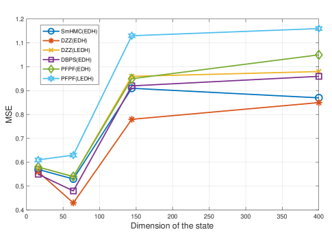
Figure 2: MSE for the different methods as the dimension of the state increases.

TABLE II: MSE, Acceptance Ratio, and execution time per step (Average over 120 trials) with Generalised hyperbolic state distribution and Poisson Observations in the Large spatial sensor networks simulation

$d$	Algorithm	Particles	MSE	Acceptance			Time(s)
				$\rho_{1}$	$\rho_{2}$	$\rho_{3}$
144	SmHMC(EDH)	300	0.91	0.05	0.006	0.73	4.3
	DBPS(EDH)	10000	0.92	0.02	0.001	0.91	4.6
	DZZ(EDH)	10000	0.78	0.06	0.001	0.78	5
	DZZ(LEDH)	300	0.96	0.12	0.015	0.57	4.9
	PFPF(EDH)	10000	0.95	NA	NA	NA	0.3
	PFPF(LEDH)	300	1.13	NA	NA	NA	40
	BPF	100000	2.02	NA	NA	NA	0.4
	UKF	NA	2.2	NA	NA	NA	0.0056
	EKF	NA	2.52	NA	NA	NA	0.0007
400	SmHMC(EDH)	300	0.87	0.02	0.0121	0.57	60
	DBPS(EDH)	10000	0.96	0.01	0.0001	0.93	67
	DZZ(EDH)	10000	0.85	0.03	0.0014	0.69	61
	DZZ(LEDH)	300	0.98	0.06	0.0176	0.65	120
	PFPF(EDH)	10000	1.05	NA	NA	NA	2.18
	PFPF(LEDH)	300	1.16	NA	NA	NA	103
	BPF	100000	2.91	NA	NA	NA	1.84
	UKF	NA	2.26	NA	NA	NA	0.09
	EKF	NA	1.96	NA	NA	NA	0.02

Fig. 2 shows the MSE of different methods with different dimension. We can find that almost DZZ(EDH) could achieve the smaller MSE with the different dimension. We visualize the true state and estimation state of different methods by Fig. 3.

Table II detailedly reports the MSE, acceptance ratio, and execution time over $120$ simulation trials. Since computational burden of different method is completely different from each other, particle numbers are adjusted to balance the accuracy and computation time. Then, we evaluate all methods. We observed that in the proposed DZZ(EDH) method, the average MSE is reduced compared with other methods. Comparing with the SmHMC(EDH), because the propeties of non-reversible Markov process and the acceptance ratio of second refinement step increases which means particles can still keep diversity after the second refinement stage, MSE of DZZ(EDH) is reduced. Comparing with the DBPS(EDH), the reason of average MSE decreased is that the mild ergodic condition of Zig-Zag method. It means we do not to set a suitable velocity refresh in the DZZ(EDH) method. DZZ(LEDH) has worse performance than DZZ(EDH). Therefore, we can indicate a conclusion. It brings additional gain in the DZZ method that we employ independently particle flow methods with every particle. Therefore, comparing with DZZ(LEDH), the DZZ(EDH) method is adopted in this situation for the reason that it is computationally much more efficient and acheives smaller average MSE than the DZZ(LEDH) method.

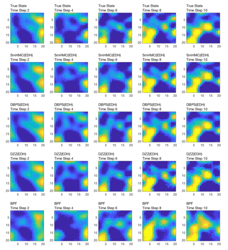
Figure 3: Illustration of the approximation result at different time steps for several Algorithms ($d=400$)

PFPF(EDH) and PFPF(LEDH) perform worse than DZZ(EDH) in the setting with same particle numbers because importance sampling is employed to close the target posterior distribution in the PFPF methods. EDH flow and LEDH flow can move particles to a special locality. In this locality, the values of target distribution are comparatively huge. However, weight degeneracy problem still disturbs the achievement of PFPF(EDH) and PFPF(LEDH) in high-dimensional situation. The MSE of bootstrap particle filtering (BPF) methods is huge even we use $1$ million particles. Besides, the condition of UKF and EKF is not be satisfied by this experiment. Therefore, their performance is not good either.

VI Conclusion

We have adopt the key idea of Zig-Zag Sampler and implemented DZZ method as the second refinement step of the Composite MH Kernel which is employed to construct the SMCMC framework. The combination of EDH and DZZ in SMCMC framework provides the minimal MSE. At the same time, compared with the state-of-the-art methods, proposed method can greatly increase acceptance ratio in the second refinement stage which means the DZZ(EDH) based SMCMC framework could explore the high-dimensional state space more efficiently.

We evaluate the proposed method in two simulation examples. In the first numerical experiment, DZZ(EDH) method can achieve the smallest MSE. However, DZZ(EDH) needs more computation time in this setting with large amount of information when the dimension is set by $64$ or $144$ among all particle filtering methods. At the same time, the proposed DZZ(EDH) method performs the most higher acceptance ratio in the refinement step which means it can keep the particles diversity. In the second numerical experiment, when the calculation time is almost the same, the proposed DZZ(EDH) method performs the smallest MSE comparing other SMCMC and SMC methods. Moreover, the acceptance ratio in the refinement step of DZZ(EDH) is still higher than that of SmHMC(EDH).

In recent years, in addition to Zig-Zag Sampler method, PDMP methods have new developments, such as Boomerange Sampler method [43]. Therefore, considering the application of the Boomerange Sampler method in the SMCMC framework is a future important research direction. Besides, we need to do more comprehensive evaluation with the numerical experiments of DZZ(EDH) method and DZZ(LEDH) method in the future. These experiments should research the influence of changes in the initial state value, variance of the state noise and observation noise, and other parameters. These experiments can further detect the robustness of the algorithm and expose the shortcomings to promote us to further improve the performance of the algorithm.

References

- [1] R. Martinez-Cantin, N. De Freitas, E. Brochu, J. Castellanos, and A. Doucet, “A Bayesian exploration-exploitation approach for optimal online sensing and planning with a visually guided mobile robot,” Autonomous Robots, vol. 27, no. 2, pp. 93–103, 2009.
- [2] D. D. Creal and R. S. Tsay, “High dimensional dynamic stochastic copula models,” Journal of Econometrics, vol. 189, no. 2, pp. 335–345, 2015.
- [3] P. J. Van Leeuwen, “Nonlinear data assimilation for high-dimensional systems,” in Nonlinear data assimilation. Springer, 2015, pp. 1–73.
- [4] M. Speekenbrink, “A tutorial on particle filters,” Journal of Mathematical Psychology, vol. 73, pp. 140–152, 2016.
- [5] M. S. Arulampalam, S. Maskell, N. Gordon, and T. Clapp, “A tutorial on particle filters for online nonlinear/non-Gaussian Bayesian tracking,” IEEE Transactions on signal processing, vol. 50, no. 2, pp. 174–188, 2002.
- [6] M. K. Pitt and N. Shephard, “Filtering via simulation: Auxiliary particle filters,” Journal of the American statistical association, vol. 94, no. 446, pp. 590–599, 1999.
- [7] R. Van Der Merwe, A. Doucet, N. De Freitas, and E. Wan, “The unscented particle filter,” Advances in neural information processing systems, vol. 13, pp. 584–590, 2000.
- [8] S. Särkkä, A. Vehtari, and J. Lampinen, “Rao-Blackwellized particle filter for multiple target tracking,” Information Fusion, vol. 8, no. 1, pp. 2–15, 2007.
- [9] M. S. Grewal, A. P. Andrews, and C. G. Bartone, “Kalman filtering,” 2020.
- [10] E. A. Wan and A. T. Nelson, “Dual extended Kalman filter methods,” Kalman filtering and neural networks, vol. 123, 2001.
- [11] E. A. Wan, R. Van Der Merwe, and S. Haykin, “The unscented Kalman filter,” Kalman filtering and neural networks, vol. 5, no. 2007, pp. 221–280, 2001.
- [12] G. Evensen, “The ensemble Kalman filter: Theoretical formulation and practical implementation,” Ocean dynamics, vol. 53, no. 4, pp. 343–367, 2003.
- [13] P. M. Djuric, T. Lu, and M. F. Bugallo, “Multiple particle filtering,” in 2007 IEEE International Conference on Acoustics, Speech and Signal Processing-ICASSP’07, vol. 3. IEEE, 2007, pp. III–1181.
- [14] A. Doucet, A. M. Johansen et al., “A tutorial on particle filtering and smoothing: Fifteen years later,” Handbook of nonlinear filtering, vol. 12, no. 656-704, p. 3, 2009.
- [15] A. Beskos, D. Crisan, A. Jasra, K. Kamatani, and Y. Zhou, “A stable particle filter for a class of high-dimensional state-space models,” Advances in Applied Probability, vol. 49, no. 1, pp. 24–48, 2017.
- [16] R. Lamberti, F. Septier, N. Salman, and L. Mihaylova, “Gradient-Based Sequential Markov Chain Monte Carlo for Multitarget Tracking With Correlated Measurements,” IEEE Transactions on Signal and Information Processing over Networks, vol. 4, no. 3, pp. 510–518, 2017.
- [17] C. Andrieu, N. De Freitas, A. Doucet, and M. I. Jordan, “An introduction to MCMC for machine learning,” Machine learning, vol. 50, no. 1, pp. 5–43, 2003.
- [18] F. Septier and G. W. Peters, “Langevin and Hamiltonian based sequential MCMC for efficient Bayesian filtering in high-dimensional spaces,” IEEE Journal of selected topics in signal processing, vol. 10, no. 2, pp. 312–327, 2015.
- [19] M. Girolami and B. Calderhead, “Riemann manifold Langevin and Hamiltonian Monte Carlo methods,” Journal of the Royal Statistical Society: Series B (Statistical Methodology), vol. 73, no. 2, pp. 123–214, 2011.
- [20] T. Xifara, C. Sherlock, S. Livingstone, S. Byrne, and M. Girolami, “Langevin diffusions and the Metropolis-adjusted Langevin algorithm,” Statistics & Probability Letters, vol. 91, pp. 14–19, 2014.
- [21] S. Livingstone and M. Girolami, “Information-geometric Markov chain Monte Carlo methods using diffusions,” Entropy, vol. 16, no. 6, pp. 3074–3102, 2014.
- [22] M. Betancourt, S. Byrne, S. Livingstone, and M. Girolami, “The geometric foundations of Hamiltonian Monte Carlo,” Bernoulli, vol. 23, no. 4A, pp. 2257–2298, 2017.
- [23] Y. Li and M. Coates, “Sequential MCMC with invertible particle flow,” in 2017 IEEE International Conference on Acoustics, Speech and Signal Processing (ICASSP). IEEE, 2017, pp. 3844–3848.
- [24] ——, “Particle filtering with invertible particle flow,” IEEE Transactions on Signal Processing, vol. 65, no. 15, pp. 4102–4116, 2017.
- [25] P. Vanetti, A. Bouchard-Côté, G. Deligiannidis, and A. Doucet, “Piecewise-deterministic Markov chain Monte Carlo,” arXiv preprint arXiv:1707.05296, 2017.
- [26] C. Sherlock and A. H. Thiery, “A discrete bouncy particle sampler,” arXiv preprint arXiv:1707.05200, 2017.
- [27] P. Fearnhead, J. Bierkens, M. Pollock, and G. O. Roberts, “Piecewise deterministic Markov processes for continuous-time Monte Carlo,” Statistical Science, vol. 33, no. 3, pp. 386–412, 2018.
- [28] J. Bierkens, A. Bouchard-Côté, A. Doucet, A. B. Duncan, P. Fearnhead, T. Lienart, G. Roberts, and S. J. Vollmer, “Piecewise deterministic Markov processes for scalable Monte Carlo on restricted domains,” Statistics & Probability Letters, vol. 136, pp. 148–154, 2018.
- [29] A. Bouchard-Côté, S. J. Vollmer, and A. Doucet, “The bouncy particle sampler: A nonreversible rejection-free Markov chain Monte Carlo method,” Journal of the American Statistical Association, vol. 113, no. 522, pp. 855–867, 2018.
- [30] J. Bierkens, P. Fearnhead, and G. Roberts, “The zig-zag process and super-efficient sampling for Bayesian analysis of big data,” The Annals of Statistics, vol. 47, no. 3, pp. 1288–1320, 2019.
- [31] S. Pal and M. Coates, “Sequential MCMC with the discrete bouncy particle sampler,” in 2018 IEEE Statistical Signal Processing Workshop (SSP). IEEE, 2018, pp. 663–667.
- [32] Y. Han and K. Nakamura, “The Influence of Velocity Refresh in Sequential MCMC with the Invertible Particle Flow and Discrete Bouncy Particle Sampler,” unpublished.
- [33] F. Septier, S. K. Pang, A. Carmi, and S. Godsill, “On MCMC-based particle methods for Bayesian filtering: Application to multitarget tracking,” in 2009 3rd IEEE International Workshop on Computational Advances in Multi-Sensor Adaptive Processing (CAMSAP). IEEE, 2009, pp. 360–363.
- [34] F. Daum and J. Huang, “Particle flow for nonlinear filters with log-homotopy,” in Signal and Data Processing of Small Targets 2008, vol. 6969. International Society for Optics and Photonics, 2008, p. 696918.
- [35] ——, “Nonlinear filters with log-homotopy,” in Signal and Data Processing of Small Targets 2007, vol. 6699. International Society for Optics and Photonics, 2007, p. 669918.
- [36] F. Daum, J. Huang, A. Noushin, and M. Krichman, “Gradient estimation for particle flow induced by log-homotopy for nonlinear filters,” in Signal Processing, Sensor Fusion, and Target Recognition XVIII, vol. 7336. International Society for Optics and Photonics, 2009, p. 733602.
- [37] F. Daum, J. Huang, and A. Noushin, “Exact particle flow for nonlinear filters,” in Signal processing, sensor fusion, and target recognition XIX, vol. 7697. International society for optics and photonics, 2010, p. 769704.
- [38] F. Daum and J. Huang, “Exact particle flow for nonlinear filters: seventeen dubious solutions to a first order linear underdetermined PDE,” in 2010 Conference Record of the Forty Fourth Asilomar Conference on Signals, Systems and Computers. IEEE, 2010, pp. 64–71.
- [39] T. Ding and M. J. Coates, “Implementation of the Daum-Huang exact-flow particle filter,” in 2012 IEEE Statistical Signal Processing Workshop (SSP). IEEE, 2012, pp. 257–260.
- [40] Y. Li, S. Pal, and M. J. Coates, “Invertible particle-flow-based sequential MCMC with extension to Gaussian mixture noise models,” IEEE Transactions on Signal Processing, vol. 67, no. 9, pp. 2499–2512, 2019.
- [41] J. Bierkens, P. Nyquist, and M. C. Schlottke, “Large deviations for the empirical measure of the zig-zag process,” arXiv preprint arXiv:1912.06635, 2019.
- [42] J. Bierkens and A. Duncan, “Limit theorems for the zig-zag process,” Advances in Applied Probability, vol. 49, no. 3, pp. 791–825, 2017.
- [43] J. Bierkens, S. Grazzi, K. Kamatani, and G. Roberts, “The boomerang sampler,” in International conference on machine learning. PMLR, 2020, pp. 908–918.