Subspace Graph Physics: Real-Time Rigid Body-Driven Granular Flow Simulation

Abstract

An important challenge in robotics is understanding the interactions between robots and deformable terrains that consist of granular material. Granular flows and their interactions with rigid bodies still pose several open questions. A promising direction for accurate, yet efficient, modeling is using continuum methods. Also, a new direction for real-time physics modeling is the use of deep learning. This research advances machine learning methods for modeling rigid body-driven granular flows, for application to terrestrial industrial machines as well as space robotics (where the effect of gravity is an important factor). In particular, this research considers the development of a subspace machine learning simulation approach. To generate training datasets, we utilize our high-fidelity continuum method, material point method (MPM). Principal component analysis (PCA) is used to reduce the dimensionality of data. We show that the first few principal components of our high-dimensional data keep almost the entire variance in data. A graph network simulator (GNS) is trained to learn the underlying subspace dynamics. The learned GNS is then able to predict particle positions and interaction forces with good accuracy. More importantly, PCA significantly enhances the time and memory efficiency of GNS in both training and rollout. This enables GNS to be trained using a single desktop GPU with moderate VRAM. This also makes the GNS real-time on large-scale 3D physics configurations (700x faster than our continuum method).

1 Introduction

Granular flows and their interactions with rigid bodies still pose several open questions. Their modeling is complex as they can experience various solid-like, fluid-like and gas-like deformations in time. Engineering applications of machine-terrain interactions include earthwork using industrial excavators, bulldozers, etc. as well as agricultural vehicles. Accurately modeling how these machines interact with granular materials can lead to the development of better training simulators and to the automation of tasks. Robot-terrain interactions are also very important in space exploration, where rovers drive over granular regolith in the reduced-gravity environments of Mars and the Moon. The entrapment of the Mars Exploration Rover Spirit in soft regolith and the tears and punctures in the Mars Science Laboratory Curiosity rover’s wheels demonstrate some of the current challenges of such reduced-gravity granular terrains. Therefore, a real-time and accurate simulation method is essential for robot mobility control, training operators, or for eventually automating aspects of these operations in the construction and space industries.

Current robot-terrain interaction models have very high computational complexity, depend on many difficult to measure parameters, and/or have insufficient predictive power. In terms of high accuracy, one current direction of research is the discrete element method (DEM), which demonstrates promise in modeling granular flows. But it is so computationally intensive as to be infeasible for online applications (comp13), and for large physical domains can be untenably expensive even in offline applications (DunDemExpK). On the other end of the complexity spectrum, several researchers today highlight the insufficient predictive power of classical terramechanics models (comp14; comp15), and their limitations to specific flow geometries (Hae20isarc), though they can be real-time. Even modern continuum methods such as material point method (MPM), that simultaneously achieve accuracy and relative efficiency, still may not be real-time for 3D configurations with existing computer processors, especially in hardware-constrained applications like planetary rovers Hae21eas.

However, data-driven methods have begun to be applied to similar (especially fluid) simulations. Some researchers (pcamg; subs1; subs2; subs3; subs4) are applying dimensionality reduction methods, such as principal component analysis (PCA) (pcaref2), to get a lower-dimensional representation of the physics data. Others (gns; mitgraph) are using graph neural networks (GNNs) (gnn0; gnn; gnn1; gnn2), such as graph networks (GNs) (gn), to learn the underlying physical dynamics more accurately. Metrics of success for these methods have to date focused on qualitative visual appearance. In the following, three important aspects of such approaches are reviewed: data, reduced data, and learning.

Data: Since machine learning physics simulation methods require hours of data at various initial and boundary conditions, numerical methods will be needed to complement and may even outweigh the use of experiments. To generate fluid simulations as training data, several lines of work have utilized smoothed particle hydrodynamics (SPH (Mon92sph)) (gns), fluid implicit particle (FLIP (Bri15flip)) (Kim19cnn; Um18ff), finite volume method (FVM) (Thu20ae), or finite difference method (FDM) (Ozb19pde). Also, some general methods such as position based dynamics (PBD (Mac14flex)) (pcamg; mitgraph), and projective dynamics (PD (Bou14pd)) (Nar16pduse; Wei16pduse) can be used for different types of material simulation (e.g. sand, snow, jelly). However, the continuum hybrid (i.e. particle and mesh-based) force-based material point method (MPM) with an accurate material model (e.g. nonlocal granular fluidity, NGF (UnsNonK)), is as one of the most accurate and efficient methods for our purpose of granular flow modeling. MPM (mpmHu) has also been recently used to produce sand simulations for the purpose of training a simulator (gns).

Reduced Data: In physics simulations, model reduction methods are utilized to capture the effective degrees of freedom of a physics system (subs1; subs2; subs3; subs4). This is with the hope to reduce both processing time and memory space usage corresponding to the system. Some work has also applied subspace methods to the equations of motion in FEM solvers (subsfem1; subsfem2). However, it is difficult to handle collisions in such approaches, and further modifications (subscol) significantly reduce its efficiency. Recent literature (pcamg) has shown that principal component analysis (PCA) could be an effective choice to capture the primary modes of elastic object deformations.

Learning: Machine learning methods have been recently shown as real-time alternatives to traditional numerical methods to learn from data. One crucial challenge here is to properly learn the underlying dynamics principles in the physical systems automatically. Some methods have been applied to differential equations such as Poisson equation (Ozb19pde). Several recent methods have also been utilized for fluid simulations, including: regression forest (Lad17regFor; Lad15regFor), multi layer perceptron (MLP) (Wie19ff; Um18ff), autoencoder (AE) (Thu20ae; Wan19ae; Mor18ae) convolutional neural network (CNN) (Kim19cnn; Tom17cnn), continuous convolution (CConv) (Umm20cc), generative adversarial network (GAN) (Xie18gan), and loss function-based method (Pra20lf). These methods are useful for a specific state of materials (gas-like, solid-like, or specifically fluid-like). They would likely need modifications to the architecture itself (not to mention additional data as well, of course) to make them work in the other states. However, graph networks (GN) (gn), a type of graph neural network (gnn), have been shown to be capable of simulating different states of materials while being simple to implement. Dynamic interaction network (mitgraph), as a GN variant, has been proposed for general simulations including elastic and rigid objects. But, it also requires additional computations and data to simulate elasto-plastic materials. In fact, the current position and velocity are no longer sufficient as inputs; additionally, the resting position and an extra network type (hierarchical modeling) are required. Recent state-of-the-art research has developed graph network simulator (GNS) (gns), which has outperformed some other recent methods (mitgraph; Umm20cc) in terms of accuracy and ease of implementation.

This research achieves accurate real-time engineering simulations of large-scale rigid body-driven granular flows. The metrics for accuracy include the positions of granular particles as well as the reaction forces on the rigid body. This is accomplished by integrating a high-accuracy machine learning approach, graph network simulator (GNS), with principal component analysis (PCA) into a subspace graph network simulator. GNS was customized to deal with subspace physics, to use a single fully-connected message passing step, and to predict interaction forces. The system is trainable via a single desktop GPU with moderate VRAM. There are two distinct contributions here: (1) extensive training data generated via an accurate MPM verified by experimental data (Hae20isarc; Hae21aero), and (2) significantly reducing the training and rollout runtime and memory usage of GNs by learning the subspace dynamics (i.e. subspace learning (SINDy)) using the reduced data obtained by applying PCA to high-dimensional physics data.

This paper is organized in the following manner: we will first provide a background on graph neural networks (GNN). Then, it will develop various modules in the training phase of the subspace graph network simulator (GNS). The paper will end by providing quantitative and qualitative rollout results compared with the ground truth MPM results. The source code of the developed algorithm is available on GitHub as referred in the context.

2 Graph Neural Networks

This section provides a background on graph neural networks (GNNs). We introduce graph machine learning, and explain the GNNs (under the field of graph machine learning) and their necessity. Furthermore, we discuss the expressive power of GNNs and introduce graph network as generalized GNNs. We also explain one limitation of GNNs and why a non-learning model reduction method can help.

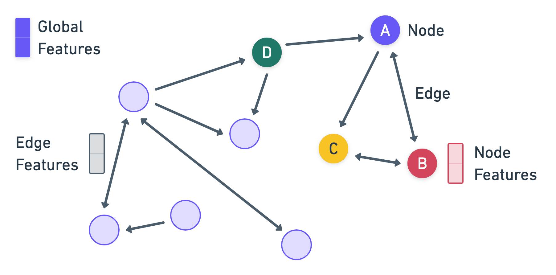
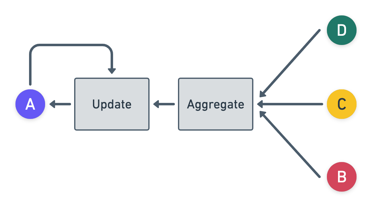
Figure 1: Left: A sample graph with nodes, directed edges, and features. Right: Illustration of one-step computational graph of node A in graph shown in Figure 1.

Graphs are general data structures for describing complex systems. Graphs are composed of entities (also known as nodes) and pairwise interactions (edges). In many cases, graph objects can have attribute (feature) information differentiating them from each other. A sample graph is shown in Figure 1(Left). Machine learning with graphs enables us to do different node-, edge-, and graph-level tasks on graph data. These include, but are not limited to, node classification (alphafold2), relation prediction (Ying_2018; bty294), graph generation (Konaklieva14Mol; StokesS20), and graph evolution (gns). Traditional machine learning pipelines require hand-engineered features extracted based on manually computed graph statistics and kernels (e.g. node degree, neighborhood overlap). These hand-engineered features are non-adaptive through a learning process, and time-consuming to process (gnnbook). Graph representation learning is an alternative approach to learning over graphs. In this approach, the aim is to automatically learn the features from encoded graph structural information.

Graph neural networks (GNNs), in their basic form, are the generalization of convolutional neural network (CNN) beyond structured grid and sequence data to non-Euclidean data (Bruna2014SpectralNA). In fact, GNNs can handle data with arbitrary size and complex topological structure, varying node ordering, and often dynamic features. In a deep message-passing framework, GNNs determine a node’s computational graph and propagate information through the graph. Below, we summarize how to propagate information across a graph to compute node features using a neural network.

2.1 Message-Passing Framework

In this framework, a graph is defined as $\lx@glossaries@gls@link{symbols}{G}{\leavevmode G}=(\lx@glossaries@gls@link{symbols}{E}{\leavevmode E},\lx@glossaries@gls@link{symbols}{V}{\leavevmode V},\lx@glossaries@gls@link{symbols}{u}{\leavevmode u})$. The $u$ is a global feature. The $\lx@glossaries@gls@link{symbols}{V}{\leavevmode V}=\{\lx@glossaries@gls@link{symbols}{v}{\leavevmode v}_{i}\}_{i=1:N^{v}}$ is a set of nodes where $\lx@glossaries@gls@link{symbols}{v}{\leavevmode v}_{i}$ are node features. The $\lx@glossaries@gls@link{symbols}{E}{\leavevmode E}=\{(\lx@glossaries@gls@link{symbols}{e}{\leavevmode e}_{i},\lx@glossaries@gls@link{symbols}{ri}{\leavevmode r_{i}},\lx@glossaries@gls@link{symbols}{si}{\leavevmode s_{i}})\}_{i=1:N^{e}}$ is a set of edges where $\lx@glossaries@gls@link{symbols}{e}{\leavevmode e}_{i}$ are edge features, ri is the index of receiver node, and si is the index of sender node. Also, $N^{e}$ and $N^{v}$ are the number of edges and nodes, respectively. Here the global, node and edge feature embeddings are $\lx@glossaries@gls@link{symbols}{hu}{\leavevmode h_{u}}=f_{u}(\lx@glossaries@gls@link{symbols}{u}{\leavevmode u})$, ${\lx@glossaries@gls@link{symbols}{hv}{\leavevmode h_{v}}}_{i}=f_{v}(\lx@glossaries@gls@link{symbols}{v}{\leavevmode v}_{i})$ and ${\lx@glossaries@gls@link{symbols}{he}{\leavevmode h_{e}}}_{i}=f_{e}(\lx@glossaries@gls@link{symbols}{e}{\leavevmode e}_{i})$, respectively, where $f(.)$’s are arbitrary functions. Note that the global and edge embeddings are only used in the graph network as a generalized message-passing framework.

Every node has its own computational graph based on its local neighbourhood. The computational graph forms a tree structure by unfolding the neighborhood around the target node (gnnbook). It can have arbitrary depth (i.e. message-passing steps). A one-step computational graph for a single node is shown in Figure 1(Right). The message-passing framework is defined upon the computational graph. A basic framework consists of arbitrary differentiable node Update and Aggregate functions as follows

$${\lx@glossaries@gls@link{symbols}{hv}{\leavevmode h_{v}}}_{i}^{(k+1)}=\text{Update}^{(k)}\left({\lx@glossaries@gls@link{symbols}{hv}{\leavevmode h_{v}}_{i}}^{(k)},\text{message}_{\lx@glossaries@gls@link{symbols}{N}{\leavevmode N}(\lx@glossaries@gls@link{symbols}{v}{\leavevmode v}_{i})}^{(k)}\right)$$ (1)

for

$$\text{message}_{\lx@glossaries@gls@link{symbols}{N}{\leavevmode N}(\lx@glossaries@gls@link{symbols}{v}{\leavevmode v}_{i})}^{(k)}=\text{Aggregate}^{(k)}\left(\{{\lx@glossaries@gls@link{symbols}{hv}{\leavevmode h_{v}}}_{j}^{(k)}|\forall\lx@glossaries@gls@link{symbols}{v}{\leavevmode v}_{j}\in\lx@glossaries@gls@link{symbols}{N}{\leavevmode N}(\lx@glossaries@gls@link{symbols}{v}{\leavevmode v}_{i})\}\right)$$ (2)

where $\text{message}_{\lx@glossaries@gls@link{symbols}{N}{\leavevmode N}(\lx@glossaries@gls@link{symbols}{v}{\leavevmode v}_{i})}^{(k)}$ is the message that is aggregated from node $\lx@glossaries@gls@link{symbols}{v}{\leavevmode v}_{i}$’s graph neighborhood, $\lx@glossaries@gls@link{symbols}{N}{\leavevmode N}(\lx@glossaries@gls@link{symbols}{v}{\leavevmode v}_{i})$, at message-passing step $k$. Also, the Update function combines the aggregated message with the previous target node embeddings.

The Update and Aggregate functions are applied per node. The Update function can be defined via a neural network (with nonlinear activation(s) to add expressiveness) in the GNN message-passing framework. There are different ways to aggregate the features, such as mean pooling in graph convolutional network (GCN) (gcn), and max pooling in GraphSage (gsage). Also, since the Aggregate function takes a set as input, the framework is permutation equivariant by design. This means that the Aggregate function output is permuted in a consistent way in response to permutations of the input (gnnbook). The expressiveness power of the Update function and the choice of the Aggregate function will be discussed later in the current section.

In this framework GNN is inductive: (1) the parameters are shared, (2) the number of parameters is sublinear within the size of graph (e.g. node features size, $|\lx@glossaries@gls@link{symbols}{V}{\leavevmode V}|$), and (3) it can be generalized to unseen nodes. Specifically, GNNs are a certain class of general neural architectures. It means that graph structure is the input to the neural architecture (instead of being part of it), and the model parameters are shared to respect the invariance properties of the input graph (pmlr-v119-you20b). GNN examples include GCN, GraphSage, and Graph Attention Network (GAT) (gat) with different message-passing architectures.

2.2 Expressiveness (Theory)

It is desirable for GNNs to have a high level of expressiveness. The expressive power of GNNs is specified as the ability to distinguish different computational graphs (i.e. graph structures). Isomorphic nodes are defined as the nodes that have the same computational graphs (i.e. same features and neighbourhood structure). GNNs are unable to distinguish two isomorphic nodes since they consider node features, not node IDs/indexes. Also, an injective function maps every unique input to a different output. The most expressive GNN maps every computational graph into different node embeddings, injectively.

Hence, the Aggregate function should be injective. That is, the expressiveness of GNNs can be characterized by the expressiveness of the Aggregate function over multisets (i.e. sets with repeating elements). For instance, GCN and GraphSage are not maximally powerful GNNs as they use non-injective mean and max pooling functions for aggregation, respectively. On the other hand, Theorem 1 recently proposed by gin indicates that a sum pooling operation is an injective function over multisets.

Theorem 1

Assume $\mathcal{X}$ is countable. There exists a function $f:\mathcal{X}\to\mathbb{R}^{n}$ so that $h(X)=\sum_{x\in X}f(x)$ is unique for each multiset $X\subset\mathcal{X}$ of bounded size. Moreover, any multiset function $g$ can be decomposed as $g(X)=\Phi\left(\sum_{x\in X}f(x)\right)$ for some function $\Phi$.

Also, the universal approximation theorem (univApprox) states that a multi-layer perceptron (MLP) with sufficiently large hidden dimensionality (i.e. from 100 to 500 nodes) and appropriate non-linearity (e.g. ReLU activation) can approximate any continuous function with an arbitrary accuracy. The Graph Isomorphism Network (GIN), developed based on the aforementioned theorems (gin), is one of the most expressive GNNs in the class of message-passing GNNs, where its expressiveness is upper bounded by Weisfeiler-Lehman Isomorphism Test. It has the following relation:

$${\lx@glossaries@gls@link{symbols}{hv}{\leavevmode h_{v}}}_{i}^{(k+1)}=\text{MLP}^{(k)}\bigg{(}{\lx@glossaries@gls@link{symbols}{hv}{\leavevmode h_{v}}}_{i}^{(k)},\text{Sum}^{(k)}\left(\{{\lx@glossaries@gls@link{symbols}{hv}{\leavevmode h_{v}}}_{j}^{(k)}|\forall\lx@glossaries@gls@link{symbols}{v}{\leavevmode v}_{j}\in\lx@glossaries@gls@link{symbols}{N}{\leavevmode N}(\lx@glossaries@gls@link{symbols}{v}{\leavevmode v}_{i})\}\right)\bigg{)}$$ (3)

Therefore, sum pooling (Sum) and MLP will be used in a generalized message-passing framework. Note that we can also add rich node features to improve the expressiveness of the GNNs.

2.3 Graph Networks

A generalized message-passing framework is known as a graph network (GN) (gn). The important aspect in graph networks is that, during message passing, in addition to node embeddings ${\lx@glossaries@gls@link{symbols}{hv}{\leavevmode h_{v}}}_{i}$, we generate the edge embeddings ${\lx@glossaries@gls@link{symbols}{he}{\leavevmode h_{e}}}_{i}$, as well as a global embedding $h_{u}$ corresponding to the entire graph. This allows the framework to easily integrate edge- and graph-level features. Also, recent work (Barcel2020TheLE) has shown GN to have benefits in terms of expressiveness compared to a standard GNN. Generating edge and global embeddings during message-passing also makes it trivial to define loss functions based on graph or edge-level classification tasks (gnnbook).

As already discussed, multi-layer perceptrons (MLPs) and element-wise sum pooling (Sum) are selected as the Update and Aggregate functions for maximal expressiveness. The message-passing neural network (MPNN, also called interaction network) architecture (Gilmer2017NeuralMP), a simplified version of the full GN architecture, will be used for the physics simulator explained in §LABEL:subsec:learning.

2.4 Limitation and Proposed Approach

GNNs might be infeasible for large-scale applications on a GPU with mid-level limits on memory (i.e. VRAM of 10-20GB). Aside from mini-batch, one solution to this is to consider linear activation functions in GNNs. This has worked well for node classification benchmark (wu2019simplifying). Using this, one can pre-process graph features on a CPU (with large memory capability) offline.

However, this will limit the expressive power of GNNs due to the lack of non-linearity in generating the embeddings. In this research, we propose applying a non-learning, CPU-runnable dimensionality reduction method, PCA, to physics graph data in order to:

1. Significantly reduce the size of graph data,

2. Reduce the required message-passing steps to only one, and

3. Eliminate the need for computationally expensive edge construction algorithms.

3 Subspace Graph Network Simulator

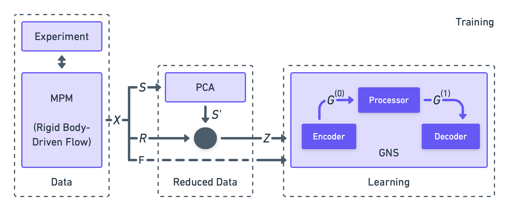
Figure 2: Training in subspace GNS. Data $X$ includes time series of flow states $S$, rigid states $R$, and interaction forces $F$. Also, $S^{\prime}$ and $Z$ are reduced flow states and reduced system states. Here, states are particle positions.

For engineering applications, the underlying physics govern the system response. A learning physics simulation can be discussed and assessed in terms of the following factors:

1. Accuracy: An accurate method ideally learns from clean and accurate datasets (§3.1).

2. Speed: A fast method can be achieved via reduced, memory-efficient data and/or by using reusable modules that can be run on modern accelerator hardware such as GPU (§3.2).

3. Generalization: Strong generalization is achievable by imposing relational inductive bias on the learning model. Models with strong inductive biases are more data efficient and can generalize much better to unseen scenarios (§LABEL:subsec:learning).

4. Differentiability: Differentiable models such as neural networks are appropriate for inverse problems (e.g. control systems).

In this section, we develop a real-time learning simulation approach for modeling rigid body-driven elasto-viscoplastic (and sometimes stress-free) granular flows. Focus on this application does not limit its potential applicability to other materials, not considered here. The approach will benefit from material point method (MPM), principal component analysis (PCA), and graph network simulator (GNS), and is decomposed to a training phase and a rollout phase. Such an approach has not been developed for granular flows before.

The training phase is illustrated in Figure 2. First, we generate training datasets via material point method (MPM) verified by experiments. Then, we apply PCA to the full data in a pre-processing step (on CPU). As a result, depending on the application, a desired quality (i.e. considering both accuracy and memory-efficiency) can determine the number of PCA modes. Finally, we train GNS (a GN model with Encoder-Processor-Decoder scheme on GPU) using data representing subspace elasto-viscoplastic granular flow. The modules shown in the figure including Data (§3.1), Reduced Data (§3.2), and Learning (§LABEL:subsec:learning) will be elaborated in the following sections.

In the rollout phase, depicted in Figure 3, we use the learned subspace model to compute the granular flow-rigid body interaction forces (on CPU). Also, the fullspace granular flows are computed in a post-processing step (on GPU) which is useful for visualization purposes. The rollout phase will be explained in §LABEL:subsec:rollout.

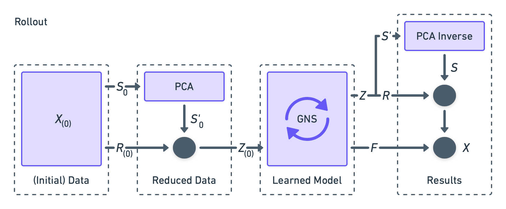
Figure 3: Rollout in subspace GNS. Initial Data $\lx@glossaries@gls@link{symbols}{X}{\leavevmode X}_{(0)}$ includes initial flow states $\lx@glossaries@gls@link{symbols}{S}{\leavevmode S}_{0}$ and (initial) rigid states $\lx@glossaries@gls@link{symbols}{R}{\leavevmode R}_{(0)}$. Also, $\lx@glossaries@gls@link{symbols}{Sp}{\leavevmode S^{\prime}}_{0}$ and $\lx@glossaries@gls@link{symbols}{Z}{\leavevmode Z}_{(0)}$ are reduced initial flow states and reduced (initial) system states. In the end, results $X$ include time series of flow states $S$, rigid states $R$, and interaction forces $F$. Also, $S^{\prime}$ and $Z$ are reduced flow states and reduced system states. Here, states are particle positions.

3.1 Data

Material point method (MPM) has been shown to provide good matching with experimental results (Hae20isarc; Hae21aero) with runtime on the order of 10 to hundreds of times real-time. Therefore, hundreds of numerical simulations can be produced for the proposed machine learning approach. Here, we generate two datasets: Excavation and Wheel. Each dataset has $\sim 75000$ data frames gathered with 60 Hz of data acquisition rate (as temporal discretization is not constrained by stability conditions, in data-driven methods). The Excavation dataset contains 250 examples with a single soil type and a blade cutting at various depths, speeds, rake angles (i.e. relative to vertical), and motion types. The Wheel dataset is slightly more complex. This includes 243 examples with soils having different internal friction angles, and wheels with various diameters operating at various normal load and slip (percentage of the wheel’s rotary motion not translating to forward linear motion). There are also multiple gravity conditions representing the Moon, Mars, and Earth. These variables are summarized in Table 1. Moreover, some examples are shown in Figure 4.

Table 1: Datasets specifications. Motion types include (1) a discrete ramp-horizontal-ramp motion, and (2) a continuous curved motion. Also, Grav., Fric., and Dia. stand for gravity, soil internal friction angle, and wheel diameter.

Dataset	Variables
Excavation	Angle [deg]	Depth [cm]	Speed [cm/s]	Motion
	{0,4,10,31,45}	{2,4,5,8,10}	{1,4,8,10,15}	{1,2}
Wheel	Grav. [$\text{m}/\text{s}^{2}$]	Fric. [deg]	Load [N]	Dia. [cm]	Slip [%]
	{1.62,3.72,9.81}	{30,37,43}	{100,164,225}	{5,15,30}	{20,40,70}

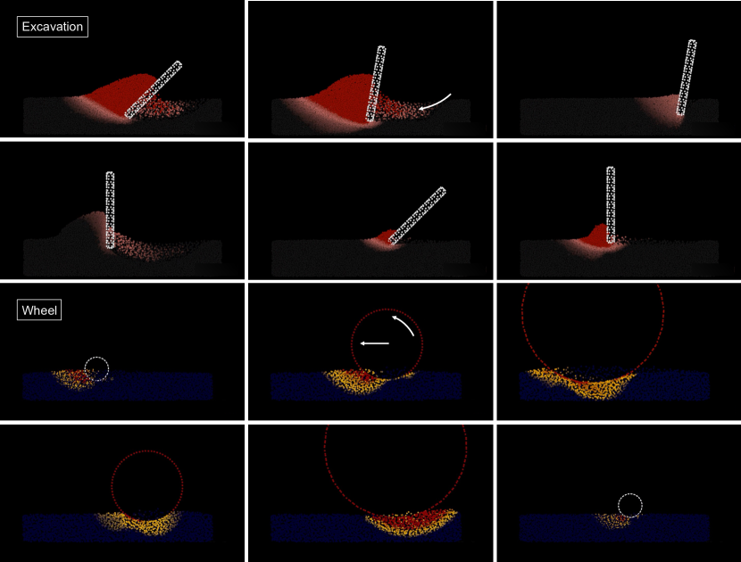
Figure 4: Side view (cross-section) of some Excavation and Wheel training examples with various initial and boundary conditions generated via MPM.

A dataset $\lx@glossaries@gls@link{symbols}{X}{\leavevmode X}=\{\lx@glossaries@gls@link{symbols}{X}{\leavevmode X}_{i}\}_{i=1:\lx@glossaries@gls@link{symbols}{c}{\leavevmode c}}$ includes $c$ examples of $\lx@glossaries@gls@link{symbols}{X}{\leavevmode X}_{i}=\{\lx@glossaries@gls@link{symbols}{S}{\leavevmode S}_{i},\lx@glossaries@gls@link{symbols}{R}{\leavevmode R}_{i},\lx@glossaries@gls@link{symbols}{F}{\leavevmode F}_{i}\}$ consisting of a time series of the positions of granular flow $\lx@glossaries@gls@link{symbols}{S}{\leavevmode S}_{i}$ and the rigid body $\lx@glossaries@gls@link{symbols}{R}{\leavevmode R}_{i}$ interacting with it, and a time series of the total interaction forces $\lx@glossaries@gls@link{symbols}{F}{\leavevmode F}_{i}$ (applied to the center of mass of the rigid body), where

$$\lx@glossaries@gls@link{symbols}{S}{\leavevmode S}_{i}=\begin{bmatrix}x_{1}^{1}&y_{1}^{1}&z_{1}^{1}&\ldots&x_{1}^{m}&y_{1}^{m}&z_{1}^{m}\\ x_{2}^{1}&y_{2}^{1}&z_{2}^{1}&\ldots&x_{2}^{m}&y_{2}^{m}&z_{2}^{m}\\ &\vdots&&\ddots&&\vdots\\ x_{n}^{1}&y_{n}^{1}&z_{n}^{1}&\ldots&x_{n}^{m}&y_{n}^{m}&z_{n}^{m}\\ \end{bmatrix}^{T}_{3\lx@glossaries@gls@link{symbols}{m}{\leavevmode m}\times\lx@glossaries@gls@link{symbols}{n}{\leavevmode n}}$$ (4)

with $m$ and $n$ as the numbers of timesteps (frames) and flow particles, respectively. In fact, each column in $\lx@glossaries@gls@link{symbols}{S}{\leavevmode S}_{i}$ represents a time series of particle positions in 3D. The $\lx@glossaries@gls@link{symbols}{R}{\leavevmode R}_{i}$ has also a similar structure. Moreover, the interaction forces $\lx@glossaries@gls@link{symbols}{F}{\leavevmode F}_{i}$ are given by

$$\lx@glossaries@gls@link{symbols}{F}{\leavevmode F}_{i}=\begin{bmatrix}F_{x}^{1}&F_{x}^{2}&\ldots&F_{x}^{m}\\ F_{y}^{1}&F_{y}^{2}&\ldots&F_{y}^{m}\\ F_{z}^{1}&F_{z}^{2}&\ldots&F_{z}^{m}\end{bmatrix}^{T}_{\lx@glossaries@gls@link{symbols}{m}{\leavevmode m}\times 3}.$$ (5)

We divide the dataset into two subsets: the training split including 90% and test split including 10% of the examples. We work with the training split in the training phase, and with the test split in the rollout phase. Also, a validation split is not required as we will use the model hyperparameters already tuned.

Note that as we separately construct the $\lx@glossaries@gls@link{symbols}{S}{\leavevmode S}_{i}$ and $\lx@glossaries@gls@link{symbols}{R}{\leavevmode R}_{i}$ data matrices, the particle types (i.e. flow, rigid/boundary, etc.) are recognizable. They are used as node features in the graph network explained in §LABEL:subsec:learning.

3.2 Reduced Data

Physical systems in MPM can be described by particles each with three coordinates (degrees of freedom) in 3D. The minimum number of particles are subject to stability conditions. Thus, such systems are often high-dimensional for large scale prolems. Note, to conserve the particle coordinates, we define the dimensions by the particles rather than the system’s degrees of freedom. However, the effective dimensions of a physical system can be far smaller than the system dimensionality.

Principal Component Analysis (PCA) is a non-parametric linear dimensionality reduction method (pcaref1; pcaref2). It provides a data-driven, hierarchical coordinate system to re-express high-dimensional correlated data. The resulting coordinate system geometry is determined by principal components. These are sometimes called bases, modes or latent variables of the data. These modes are uncorrelated (orthogonal) to each other, but have maximal correlation with the observations (pcabook). Particularly, the goal of this method is to compute a subset of ranked principal components to summarize the high-dimensional data while retaining trends and patterns. PCA, as a model reduction method, can capture the effective dimensions of the physicals system. In fact, PCA enables us to calculate the complexity of the system. It should be noted that both the strength and weakness of PCA is that it is a non-parametric method. In cases where standard PCA fails due to the existence of non-linearly in data, kernel PCA (kernelpca) can be used. Compared to an autoencoder neural network, kernel PCA still does not require learning/optimization and prior specification of size of the latent space.

Reduced Data Computation: We aim to apply PCA to the granular flow data, and pass the rigid body as is ((pcamg)). Therefore, we compute the PCA transformation matrix $\lx@glossaries@gls@link{symbols}{U}{\leavevmode U}_{\lx@glossaries@gls@link{symbols}{n}{\leavevmode n}\times\lx@glossaries@gls@link{symbols}{r}{\leavevmode r}}$ where $r$ is the number of modes we select, and the data matrix is $\lx@glossaries@gls@link{symbols}{S}{\leavevmode S}_{\text{train}}$ including the flow states of each example in the training split as follows

$$\text{<span title="" class="ltx\_glossaryref ltx\_font\_italic">S</span>}{}_{\text{train}}=[\begin{array}{cc}\text{<span title="" class="ltx\_glossaryref ltx\_font\_italic">S</span>}{}_1& \text{<span title="" class="ltx\_glossaryref"><span class="ltx\_text ltx\_glossary\_name"><xmath xmlns="http://dlmf.nist.gov/LaTeXML" id="S3.E6.m1.1.1.1.1.1.1.2.1.1d" xref="S3.E6.m1.1.1.2.cmml"><xmtok role="UNKNOWN" font="italic" id="S3.E6.m1.1.1.1.1.1.1.2.1.1e" xref="S3.E6.m1.1.1.2.1.cmml">S</xmtok></xmath></span></span>}\end{array}$$ (6)