1 A Direct FPT Approach

In this section, we give direct FPT streaming algorithms for for the same cases as Theorem LABEL:TheoremPiFree. This is motivated by the fact that Chitnis and Cormode [ChitnisTheory] found a direct FPT algorithm for Vertex Cover using $\O(2^{k})$ passes and only $\Ot(k)$ space in contrast to the kernel of Chitnis et al. [ChitnisEsfandiariSampling] using one pass and $\Ot(k^{2})$ space. Therefore, we aim to explore the pass/memory trade-off for as well.

1.1 $P_{3}$-free DeletionP3-free Deletion

We start with the scenario where $\Pi=\{P_{3}\}$, which means we consider the problem Cluster Vertex Deletion [VC]. The general idea of the algorithm is to branch on what part of the given vertex cover should be in the solution. For managing the branching correctly, we use a black box enumeration technique also used by Chitnis and Cormode [ChitnisTheory].

Definition 1.1.

([ChitnisTheory, Definition 9]) Let $U=\{u_{1},u_{2},\ldots,u_{n}\}$ and $k\leq n$. Let $\U_{\leq k}$ denote the set of all $\sum_{i=0}^{k}{|U|\choose i}$ subsets of $U$ which have at most $k$ elements, and let $\textsc{Dict}_{\U_{\leq k}}$ be the dictionary ordering on $\U_{\leq k}$. Given a subset $X\in\U_{\leq k}$, let $\textsc{Dict}_{\U_{\leq k}}(\textsc{Next}(X))$ denote the subset that comes immediately after $X$ in the ordering $\textsc{Dict}_{\U_{\leq k}}$. We denote the last subset in the dictionary order of $\U_{\leq k}$ by $\textsc{Last}(\U_{\leq k})$, and similarly the first subset as $\textsc{First}(\U_{\leq k})$, and use the notation that $\textsc{Dict}_{\U_{\leq k}}(\textsc{Next}(\textsc{Last}(\U_{\leq k})))=\spadesuit$. Similarly, we define $\U_{k}$ as the set of all ${|U|\choose k}$ subsets of $U$ with exactly $k$ elements, and analogously define the dictionary ordering on this set.

In a branch, we first check whether the ‘deletion-free’ part of the vertex cover ($Y$) contains a $P_{3}$, which invalidates a branch. Otherwise, what remains is some case analysis where either one or two vertices of a $P_{3}$ lie outside the vertex cover, for which we deterministically know which vertices have to be removed to make the graph $P_{3}$-free. We illustrate this step in Figure 1. Case 1 and 2 have only one option for removal of a vertex. After Case 1 and 2 no longer occur, we can find Case 3 occurrences and show that we can delete all but one of the vertices in such an occurrence. So, if this process can be executed in a limited number of passes, the algorithm works correctly.

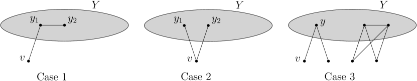
Figure 1: The different cases how a $P_{3}$ can exists with respect to $Y$, part of the vertex cover. Notice that the case where the entire $P_{3}$ is contained in $Y$ is not included here. Case 3 assumes there are no Case 1 or Case 2 $P_{3}$’s in the graph anymore.

We give the full algorithm in Algorithm 1.

[ht] $P_{3}$-free Deletion(Graph $G=(V,E)$ given as a stream in the AL model, integer $\ell$, Vertex Cover $X\subseteq V(G)$) [1] $S\leftarrow\textsc{First}(\X_{\leq\ell})$ $S\in\X_{\leq\ell},S\neq\spadesuit$ $Y\leftarrow X\setminus S$ $Y$ is the part of the vertex cover not in the solution $S$ $S^{\prime}\leftarrow S$ If $S^{\prime}$ ever exceeds size $\ell$, move to the next $S$ $P\leftarrow\textsc{First}(\Y_{2})$ $P=(y_{1},y_{2})\in\Y_{2},P\neq\spadesuit$ We enumerate all pairs in $Y$ Vertex $v\in Y\setminus P$ If $v$ and $P$ form a $P_{3}$, $Y$ is invalid, move to the next $S$ Requires a pass$P\leftarrow\textsc{Dict}_{\Y_{2}}(\textsc{Next}(P))$ $P\leftarrow\textsc{First}(\Y_{2})$ $P=(y_{1},y_{2})\in\Y_{2},P\neq\spadesuit$ We enumerate all pairs in $Y$ $y_{1}y_{2}$ is an edge Vertex $v\in V\setminus(X\cup S^{\prime})$ in the stream Either $vy_{1}$ or $vy_{2}$ is present and the other is not $S^{\prime}\leftarrow S^{\prime}\cup\{v\}$Vertex $v\in V\setminus(X\cup S^{\prime})$ in the stream Both $vy_{1}$ and $vy_{2}$ are present $S^{\prime}\leftarrow S^{\prime}\cup\{v\}$ $P\leftarrow\textsc{Dict}_{\Y_{2}}(\textsc{Next}(P))$ $y\in Y$ $b\leftarrow False$ Vertex $v\in V\setminus(X\cup S^{\prime})$ in the stream The edge $vy$ is present and $b=False$ $b\leftarrow True$ The edge $vy$ is present $S^{\prime}\leftarrow S^{\prime}\cup\{v\}$ $|S^{\prime}|\leq\ell$ $S^{\prime}$ $S\leftarrow\textsc{Dict}_{\X_{\leq\ell}}(\textsc{Next}(S))$ NO No branch resulted in a solution

To limit the number of passes, the use of the AL model is crucial. Notice that for every pair of vertices $y_{1},y_{2}$ in the vertex cover, we can identify a Case 1 or 2 $P_{3}$ of Figure 1, or these cases but with $v$ in the vertex cover as well, in a constant number of passes. This is because we can first use a pass to check the presence of an edge between $y_{1}$ and $y_{2}$, and afterwards use a pass to check the edges of every other vertex towards $y_{1}$ and $y_{2}$ (which are given together because of the AL model). This means we can find $P_{3}$’s contained in the vertex cover or corresponding to Case 1 or 2 $P_{3}$’s in $\O(K^{2})$ passes total. The remaining Case 3 can be handled in $\O(K)$ passes from the viewpoint of each $y\in Y$. So this algorithm takes $\O(2^{K}K^{2})$ passes (including branching).

Theorem 1.2.

We can solve Cluster Vertex Deletion [VC] in the AL streaming model using $\O(2^{K}K^{2})$ passes and $\O(K\log n)$ space.

Proof 1.3.

We claim that Algorithm 1 does exactly this.

Let us first reason that the number of passes and memory use are as stated. Let $X$ be the provided vertex cover, and let $|X|=K$. The number of different sets $S$ can take is bounded by $2^{K}$. The first and second loop enumerate all pairs of vertices in the vertex cover, and use a single pass per pair to detect a $P_{3}$, which gives us at most $K^{2}$ passes. The last loop enumerates all $K$ vertices in the vertex cover and uses one pass per iteration. Therefore, the total number of passes is bounded by $\O(2^{K}K^{2})$.

No set in memory exceeds $\O(K\log n)$ bits, so the stated memory complexity is correct.

Let us now show the correctness of the algorithm. The main idea of the algorithm is to branch on what part of the vertex cover is contained in the solution $S^{\prime}$. This is modelled through the use of the sets $Y$ and $S$, where in each branch, we cannot add vertices in $Y$ to $S^{\prime}$. Therefore, we first check whether $Y$ fully contains a $P_{3}$, and if one is found we stop, as we may not delete any vertex of this $P_{3}$ in this branch. For a fixed pair $(v,w)$ in the vertex cover, checking for a $P_{3}$ that contains $v$ and $w$ only takes one pass because the only necessary information is the adjacencies of $v$ and $w$ towards another vertex, which is provided in the stream local to that vertex (see also Case 1 and Case 2 in the following analysis).

What remains is a careful analysis of the different cases of the structure of $P_{3}$’s with respect to $Y$. An illustration is given in Figure 1. The loop of line 1.1 considers all pairs of vertices in $Y$. There are two cases we are interested in: Case 1 and Case 2 in Figure 1. If we look at a single pair of vertices $y_{1}$ and $y_{2}$ either there is an edge between them (Case 1) or a non-edge (Case 2). These two vertices can then form a $P_{3}$ with any vertex outside $Y$ in a very specific manner, which the algorithm looks for. It is then trivial that the one vertex outside $Y$ has to be removed to make the graph $P_{3}$ free if a $P_{3}$ is found.

If there are no Case 1 or Case 2 $P_{3}$’s in the graph any more, we move on to Case 3. Note that this is the only remaining way a $P_{3}$ can be in the graph at all, because $Y\subseteq X$ is (part of) a vertex cover. In Case 3 at first it seems undecided which of the two vertices outside $Y$ to remove, as one might lead to a solution and the other not. Let $y_{1},v,w$ form a Case 3 $P_{3}$, where $y_{1}\in Y$. Let us consider the scenario where $v$ has another adjacency $y_{2}\in Y$. Because there are no Case 2 $P_{3}$’s, $y_{1}$ and $y_{2}$ must be adjacent. Because there are no Case 1 $P_{3}$’s, $w$ must now also be adjacent to $y_{2}$. This means the structure extends as illustrated on the right in Case 3 in Figure 1. We can observe that we need to delete all but one of the vertices attached to $y$, which is what the algorithm does. It does not matter which vertex we do not delete, as this vertex forms triangles if it has multiple adjacencies. Therefore, after these cases have all been handled, no induced $P_{3}$’s remain in the graph. If during the process $S^{\prime}$ never exceeded size $\ell$, this means we have found a solution; otherwise, we move on to the next branch.

By the above reasoning, if there exists a solution of size at most $\ell$ for the Cluster Vertex Deletion [VC] problem, then this solution contains some subset of the vertex cover $X$, which corresponds to some branch in the algorithm. As the removal of vertices is deterministic in each branch (as in, the solution must contain these vertices), and there exists a solution, the algorithm must find a solution too in that branch. If there exists no solution of size at most $\ell$, then there exists no subset of vertices $S^{\prime}$ such that $G\setminus S^{\prime}$ is induced $P_{3}$ free, and so in each branch of the algorithm $S^{\prime}$ will exceed size $\ell$ at some point, which results in the algorithm returning NO.

Let us stress some details. The use of the AL model is crucial, as it allows us to locally inspect the neighbourhood of a vertex when it appears in the stream. The same approach would require more memory or more passes in other models to accomplish this result. Also note that we could implement this algorithm in a normal setting (the graph is in memory, and not a stream) to get an algorithm for Cluster Vertex Deletion [VC] with a running time of $\O(2^{K}\cdot K^{2}\cdot(n+m))$.

1.2 $H$-free DeletionH-free Deletion

We now consider a more generalized form of , where $\Pi=\{H\}$, a single graph. Unfortunately, the approach when $H=P_{3}$ does not seem to carry over to this case, because the structure of a $P_{3}$ is simple and local.

Theorem 1.4.

We can solve $H$-free Deletion [VC] in $2^{O(K^{2})}\,\mathrm{poly}(n,|V(H)|)$ time, where $H$ contains at least one edge and $K$ is the size of the vertex cover.

Proof 1.5.

Let $X$ be a vertex cover of $G=(V,E)$ of size $K$. Then $G[V\setminus X]$ has no edges and thus does not contain an occurrence of $H$. It follows that there is a solution of size at most $K$. Now call two vertices of $V\setminus X$ equivalent if their neighborhood in $X$ is the same. This yields $2^{K}$ equivalence classes. Observe that vertices in an equivalence class are interchangeable with respect to a solution for $H$-free Deletion [VC]: one can be exchanged for another without changing the validity of the solution. Hence, we may select the vertices of a solution from the first $K$ vertices of an equivalence class. This means that there is a set of at most $(2^{K}+1)K$ vertices in $G$ that form a superset of some solution. Then we can enumerate all possible such solutions, which have size at most $K$, in $2^{O(K^{2})}$ time. The validity of a solution can be checked in $2^{O(K\log K)}\mathrm{poly}(n,|V(H)|)$ time through the algorithm of Abu-Khzam [Abu-Khzam14].

In order to analyze the complexity with respect to $H$ more precisely and to obtain a streaming algorithm, we present a different algorithm that works off a simple idea. We branch on the vertex cover, and then try to find occurrences of $H$ of which we have to remove a vertex outside the vertex cover. We branch on these removals as well, and repeat this find-and-branch procedure. In an attempt to keep the second branching complexity low, we start by searching for occurrences of $H$ such that only one vertex lies outside the vertex cover, and increase this number as we find no occurrences. For clarity, we present the occurrence detection part of the algorithm first, a procedure we call FindH. Note that this is not (yet) a streaming algorithm.

[tb] The procedure FindH. [1] FindHsolution set $S$, forbidden set $Y\subseteq X$, integer $i$ Set $O$ of $i$ vertices of $H$ that can be outside $X$ Check non-edges Denote $H^{\prime}=H\setminus O$ Occurrence of $H^{\prime}$ in $Y$ Check $\O({|X|\choose|H|-i}(|H|-i)!)$ options $S^{\prime}\leftarrow\emptyset$, $O^{\prime}\leftarrow O$ Vertex $v\in V\setminus(S\cup X)$ Check the edges/non-edges towards $H^{\prime}\in Y$ $v$ is equivalent to some $w\in O^{\prime}$ for $H^{\prime}$ $S^{\prime}\leftarrow S^{\prime}\cup\{v\}$, $O^{\prime}\leftarrow O^{\prime}\setminus\{w\}$ $O^{\prime}=\emptyset$ $S^{\prime}$ We found an occurrence of $H$ $\emptyset$ No occurrence of $H$ found

Lemma 1.6.

Given a graph $G$ with vertex cover $X$, graph $H$ with at least one edge, and sets $S$, $Y\subseteq X$, and integer $i$, Algorithm 1.5 finds an occurrence of $H$ in $G$ that contains no vertices in $S$ and $X\setminus Y$ and contains $|V(H)|-i$ vertices in $Y$. It runs in $\O\left({h\choose i}[i^{2}+{K\choose h-i}(h-i)!((h-i)^{2}+Kn+(h-i)in)]\right)$ time, where $|V(H)|=h$ and $|X|=K$.

Proof 1.7.

The correctness of the algorithm follows from the enumeration of all possibilities.

Let us analyse the running time. Checking all possible sets $O$ takes $\O({h\choose i}i^{2})$ time resulting in at most $\O({h\choose i})$ options for $O$. There are at most $\O({K\choose h-i}(h-i)!)$ options for $H^{\prime}$ in $Y$: checking all of them costs $\O({K\choose(h-i)}(h-i)!(h-i)^{2})$ time. Then we take $\O((K+(h-i)i)n)$ time to, for each vertex, save adjacencies to $H^{\prime}$, and check whether it matches on of those in $O$. The $(h-i)$ factor is for checking adjacencies towards $H^{\prime}$. Therefore, the running time of FindH is $\O\left({h\choose i}[i^{2}+{K\choose h-i}(h-i)!((h-i)^{2}+Kn+(h-i)in)]\right)$.

Now let us give the complete FPT algorithm for $H$-free Deletion [VC] (not in the streaming setting), see Algorithm 1.7.

[!htp] $H$-free Deletion FPT(Graph $G=(V,E)$, integer $\ell$, Vertex Cover $X\subseteq V(G)$) [1] Partition of $X$ into $S,Y$ where $|S|\leq\ell$ $H$ is not contained in $Y$ Check all $\O({|X|\choose|H|}|H|!)$ options Branch$S$, $Y$, $1$ YES If any returns YES, we also return YESNO

Branchsolution set $S$, forbidden set $Y\subseteq X$, integer $i$ $B\leftarrow$ FindH$S$, $Y$, $i$ Try to find an $H$ with $i$ vertices outside $Y$ $B=\emptyset$ and $i=|H|$ YES $B=\emptyset$ Branch$S$, $Y$, $i+1$ No $H$ found $|S|=\ell$ NO Found an $H$ but cannot remove it $v\in B$ Branch$S\cup\{v\}$, $Y$, $i$ YES

Together with Lemma 1.6 we can analyse the performance of Algorithm 1.7 in its entirety.

Theorem 1.8.

Algorithm 1.7 is an FPT algorithm for $H$-free Deletion [VC] using $\O(2^{K}h^{K}K^{h+1}h!h^{2}n)$ time or alternatively $\O(2^{K}h^{K}K!Kh!h^{2}n)$ time, where $|V(H)|=h$ and $H$ contains at least one edge.

Proof 1.9.

Let us first go into detail on the correctness of the algorithm. Assume the algorithm returns YES for some instance $G,H,\ell,X$ where $|X|=K$ and $|V(H)|=h$. The only way the algorithm returns YES, is if in some partition of $X$ into $S$ and $Y$ the Branch function returns YES. The Branch function only returns YES if any recursive call returns YES, or when $B=\emptyset$ and $i=h$. As the latter is the only base case, this must have occurred for this instance. As $i$ starts at $1$ and is only ever incremented, we can conclude that for every $i$ at some point $B=\emptyset$ while $|S|\leq\ell$. The algorithm calls on FindH for every $i$ to find if there is an occurrence of $H$ with $i$ vertices outside of $Y\cup S$ and $|V(H)|-i$ vertices in $Y$. By Lemma 1.6, FindH correctly finds occurrences of $H$ where $i$ vertices are outside $Y$. As the algorithm returned YES, FindH must have returned an empty set for each $i$ at some point, and so no occurrences of $H$ are present in the graph $G[V\setminus S]$ (otherwise, such an occurrence must have $i$ vertices outside $Y\cup S$ for some $i$). This means that the algorithm is correct in returning YES.

For the other direction, assume that for an instance $G,H,\ell,X$ where $|X|=K$ there exists a smallest set $S_{opt}$ such that $G[V\setminus S_{opt}]$ is $H$-free and $|S_{opt}|\leq\ell$. Then $S_{opt}$ must contain some part of the vertex cover $X$, and as we enumerate all possibilities, the algorithm considers this option. As $G[V\setminus S_{opt}]$ is $H$-free, clearly, for every set $B$ the function FindH finds, at least one vertex in $B$ is also in $S_{opt}$. As we branch on each possibility of the vertices in $B$, the algorithm also considers exactly the option where the set $S$ in the algorithm is a subset of $S_{opt}$. This means there is a branch where the algorithm terminates with $S=S_{opt}$, which means it returns YES as $G[V\setminus S_{opt}]$ is $H$-free. We conclude that the algorithm solves $H$-free Deletion correctly.

Let us analyse the running time of the algorithm. There are $\O(2^{K})$ possible partitions of $X$ into $S$ and $Y$. Checking whether $H$ is contained in $Y$ takes $\O({K\choose h}h!h^{2})$ time. Because $H$ contains at least one edge, we can assume that $\ell\leq K$, as otherwise $X$ is a trivial solution. The function Branch is called in worst case $\O(h^{\ell})=\O(h^{K})$ times (branching on at most $h$ vertices each time). FindH is called at most once for every $i$ in every branch. By Lemma 1.6, FindH runs in $\O\left({h\choose i}[i^{2}+{K\choose h-i}(h-i)!((h-i)^{2}+Kn+(h-i)in)]\right)$ time. Here is where there is some variance in how we round these complexities, namely when concerning e.g. ${K\choose h}$. This is because we can both say ${K\choose h}=\O(K^{h})$, and ${K\choose h}=\O(K!)$. Which of these is a tighter bound comes down to the value of $h$ in comparison to $K$. The total complexity of the algorithm comes down to

$${\textstyle\O\left(2^{K}\left({K\choose h}h!h^{2}+h^{K}\sum_{i=1}^{h}{h\choose i}[i^{2}+{K\choose h-i}(h-i)!((h-i)^{2}+Kn+(h-i)in)]\right)\right)}$$

time, which we can shorten to either $\O(2^{K}h^{K}K^{h+1}h!h^{2}n)$ or $\O(2^{K}h^{K}K!Kh!h^{2}n)$ time.

Before we go into the translation of Algorithm 1.7 to the streaming model, let us discuss one of its shortcomings. A large part of the complexity of the algorithm comes from the twofold branching (on the vertex cover and on the possible deletions), but next to this, the function FindH largely contributes to the complexity. We can ask ourselves whether or not this function can be made more efficient. This means we are interested in more efficient induced subgraph finding, which is also called induced subgraph isomorphism. This problem has been studied in the literature, with varying degrees of success. There are a couple of main issues with regard to applying such results to this algorithm. For one, many results focus on specific graph structures, e.g. finding $r$-regular induced subgraphs [RegularSubgraphFind]. These results do not help us as we are interested in general structures. Another problematic factor is the common approach of using matrix multiplication. The issue with matrix multiplication is that it does not translate well to the streaming model, as often matrices require at least super-linear memory. An example of such an algorithm can be found in [FindCountSmallSubgraphsEfficiently].

FindH is adaptable to the streaming setting, as is the complete algorithm, see Algorithm 1.9. All the actions FindH takes are local inspection of edges, and many enumeration actions, which lend itself well to usage of the AL streaming model. The number of passes of the streaming version is closely related to the running time of the non-streaming algorithm. This then leads to the full find-and-branch procedure.

It should be clear that the functionality of Algorithm 1.9 is the same as that of Algorithm 1.7, but translated to the streaming model using as little memory as possible. Once again we make use of dictionary orderings, see Definition 1.1 for the formal definition.

[!htp] $H$-free Deletion Stream(Graph $G=(V,E)$ in the AL model, integer $\ell$, Vertex Cover $X\subseteq V(G)$) [1] $S\leftarrow\textsc{First}(\X_{\leq\ell})$ $S\in\X_{\leq\ell},S\neq\spadesuit$ $Y\leftarrow X\setminus S$ $S^{\prime}\leftarrow S$ $\neg$ Check$H$,$Y$ Branch$S^{\prime}$, $Y$, $1$ YES If any returns YES, we also return YES$S\leftarrow\textsc{Dict}_{\X_{\leq\ell}}(\textsc{Next}(S))$ NO

Checkset to find $H$, search space $Y$ $P\leftarrow\textsc{First}(\Y_{|H|})$ $P\in\Y_{|H|},P\neq\spadesuit$ Permutation $p$ of the vertices of $H$ Use a pass to check if $p$ matches $P$ Go to the next $p$ if some edges do not match $p$ matches $P$ YES $P\leftarrow\textsc{Dict}_{\Y_{|H|}}(\textsc{Next}(P))$ NO

Branchsolution set $S$, forbidden set $Y\subseteq X$, integer $i$ $B\leftarrow$ FindH$S$, $Y$, $i$ Try to find an $H$ with $i$ vertices outside $Y$ $B=\emptyset$ and $i=|H|$ YES $B=\emptyset$ Branch$S$, $Y$, $i+1$ No $H$ found $|S|=\ell$ NO Found an $H$ but cannot remove it $v\in B$ Branch$S\cup\{v\}$, $Y$, $i$ YES

FindHsolution set $S$, forbidden set $Y\subseteq X$, integer $i$ Set $O$ of $i$ vertices of $H$ that can be outside $Y$ Check non-edges in $H$ Denote $H^{\prime}=H\setminus O$ $P\leftarrow\textsc{First}(\Y_{|H^{\prime}|})$ $P\in\Y_{|H^{\prime}|},P\neq\spadesuit$ Permutation $p$ of the vertices of $H^{\prime}$ Use a pass to check if $p$ matches $P$ $p$ matches $P$ $S^{\prime}\leftarrow\emptyset$, $O^{\prime}\leftarrow O$ Vertex $v\in V\setminus(S\cup Y)$ Check the edges/non-edges towards $H^{\prime}\in Y$ $v$ is equivalent to some $w\in O^{\prime}$ for $H^{\prime}$ $S^{\prime}\leftarrow S^{\prime}\cup\{v\}$, $O^{\prime}\leftarrow O^{\prime}\setminus\{w\}$ $O^{\prime}=\emptyset$ $S^{\prime}$ We found an $H$ occurrence $P\leftarrow\textsc{Dict}_{\Y_{|H^{\prime}|}}(\textsc{Next}(P))$ $\emptyset$ No occurrence of $H$ found

Theorem 1.10.

We can solve $H$-free Deletion [VC] in the AL model, where $H$ contains at least one edge, using $\O(2^{K}h^{K+2}K^{h}h!)$ or alternatively $\O(2^{K}h^{K+2}K!h!)$ passes and $\O((K+h^{2})\log n)$ space, where $|V(H)|=h$.

Proof 1.11.

The algorithm in question is Algorithm 1.9.

Let it be clear from the algorithm that the approach to solving $H$-free Deletion has not changed from Algorithm 1.7. Therefore, if the graph stream is handled correctly, we can conclude that $H$-free Deletion is solved correctly. As we have $H$ in memory, we only require to use passes of the stream to determine (parts of) $X$ and $G$. The dictionary orderings require no passes because we have the vertices of $X$ in memory. The only places where we require passes of the stream thus are when concerning edges of the vertex cover, and edges/vertices in the rest of the graph ($V\setminus X$). Notice that at such points in Algorithm 1.9 we correctly mention the use of a pass. The loop over all vertices in $V\setminus(S\cup Y)$ only requires one pass because of the use of the AL model. Therefore, the algorithm is a correct adaptation of Algorithm 1.7 to the streaming model.

What remains is to analyse the number of passes and memory use. Let us analyse the memory use per function. The entire algorithm keeps track of the vertex cover $X$, and the forbidden graph $H$. Denote $|X|=K$ and $|V(H)|=h$. The vertex cover uses $\Ot(K)$ bits, and because we save the entirety of $H$ we use $\Ot(h^{2})$ bits. The main function uses the set $S$ of at most $\ell$ elements of $X$, likewise $S^{\prime}$, and the set $Y$ of size $\O(K)$. The function Check uses a set $P$ of $h$ elements, a permutation $p$ of $h$ elements, and $\O(1)$ bits to check if $p$ matches $P$, as it can stop when it does not match. The function Branch uses a set $B$ of at most $h$ elements and increases the size of the set $S$, but only when it does not exceed $\ell$ elements. The function FindH uses sets $O$, $H^{\prime}$, $P$, $O^{\prime}$, $p$, all of at most $h$ vertices. It also uses $\O(1)$ bits to check if $p$ matches $P$, and $\O(h)$ bits to save the adjacencies to $H^{\prime}$ to check if some vertex matches one in $O^{\prime}$. $S^{\prime}$ can only contain an element for each element in $O^{\prime}$. Therefore, $S^{\prime}$ contains at most $h$ elements.

We can conclude the memory use of a single branch is bounded by $\O((K+h^{2})\log n)$ bits. However, in this algorithm we branch on $h$ options, which is not a constant. Therefore, to be able to return out of recursion when branching and continue where we left off, we need to save the set $B$, or recompute it when we return. Saving the sets $B$ takes $\Ot(hK)$ bits because we have at most $K$ active instances. Alternatively, recomputing $B$ adds a factor $h$ to the number of passes. Seeing as we aim to be memory efficient, we opt for this second option here.

The number of passes used by the algorithm is closely aligned with the running time of Algorithm 1.7. There are only three places in which we use a pass of the stream, namely, line 14 in the function Check, and line 32 and line 35 in the function FindH. The loop of line 35 requires only one pass because the stream is given in the Adjacency List model. The number of passes is clearly dominated by the number of times the passes in line 32/35 are used. Now we can use the same analysis as for Algorithm 1.7, but make some nuances in the running time, as we have to distinguish running time which leads to more passes and running time which will be ‘hidden’ in the allowed unbounded computation. Consider the running time of FindH, as given by Lemma 1.6, $\O\left({h\choose i}[i^{2}+{K\choose h-i}(h-i)!((h-i)^{2}+(h-i)in)]\right)$. The running time factors $i^{2}$ and $(h-i)^{2}$ are checks over some amount of edges, which will be hidden by the unbounded computation. The factor $(h-i)in$ comes from the finding of vertices that fit the current form of $H$, and can be done in one pass, which means this factor falls away as well. We now have that the FindH function costs us $\O\left({h\choose i}{K\choose h-i}(h-i)!\right)$ passes. This can be shortened to $\O(K^{h}h!)$ by expanding the ${h\choose i}$ factor, and bounding ${K\choose h-i}=\O(K^{h})$. We can also bound this by $\O(K!h!)$ as discussed before. As FindH is called for every $1\leq i\leq h$ in every branch, we get an extra $h$ factor in the total number of passes. Another factor $h$ is added for recomputing $B$ when returning out of recursion at every step. This means the total number of passes comes down to either $\O(2^{K}h^{K+2}K^{h}h!)$ or $\O(2^{K}h^{K+2}K!h!)$.

1.3 Towards $\Pi$-free DeletionTowards Pi-free Deletion

An issue with extending the previous approach to the general $\Pi$-free Deletion problem is the dependence on the maximum size $h$ of the graphs $H\in\Pi$. Without further analysis, we have no bound on $h$. However, we can look to the preconditions used by Fomin et al. [jansenPaper] on $\Pi$ in e.g. Theorem LABEL:TheoremPiFree to remove this dependence.

The first precondition is that the set $\Pi^{\prime}\subseteq\Pi$ of graphs that are vertex-minimal with respect to $\Pi$ have size bounded by a function in $K$, the size of the vertex cover. That is, for these graphs $H\in\Pi^{\prime}$ we have that $|V(H)|\leq p(K)$, where $p(K)$ is some function. We can prove that it suffices to only remove vertex-minimal elements of $\Pi$ to solve $\Pi$-free Deletion, see Lemma 1.12. Note that Fomin et al. [jansenPaper] require that this is a polynomial, we have no need to demand this.

Lemma 1.12.

Let $\Pi$ be some graph property, and denote the set of vertex-minimal graphs in $\Pi$ with $\Pi^{\prime}$. Let $G$ be some graph and $S\subseteq V(G)$ some vertex set. Then $G[V(G)\setminus S]$ is $\Pi$-free if and only if $G[V(G)\setminus S]$ is $\Pi^{\prime}$-free.

Proof 1.13.

Assume the preconditions in the lemma, and assume that $G[V(G)\setminus S]$ is not $\Pi^{\prime}$-free. As $\Pi^{\prime}\subseteq\Pi$, clearly, $G[V(G)\setminus S]$ is not $\Pi$-free.

Now assume that $G[V(G)\setminus S]$ is $\Pi^{\prime}$-free. Assume there is some $H\in\Pi$ such that $H\in G[V(G)\setminus S]$ (that is, $H$ is isomorphic to an induced subgraph of $G[V(G)\setminus S]$). As the graph is $\Pi^{\prime}$-free, $H$ is a non-vertex-minimal graph with respect to $\Pi$. By definition of vertex-minimal, removal of a specific set of one or more vertices of $H$ results in a vertex-minimal graph $I\in\Pi^{\prime}$. But if we ignore the same set of vertices in $H\in G[V(G)\setminus S]$, clearly, $I\in G[V(G)\setminus S]$. This contradicts our assumption that $G[V(G)\setminus S]$ is $\Pi^{\prime}$-free. Therefore, there cannot be a $H\in\Pi$ such that $H\in G[V(G)\setminus S]$, which means that $G[V(G)\setminus S]$ is $\Pi$-free.

If we also assume that we know the set $\Pi^{\prime}$, we obtain the following result.

Theorem 1.14.

If $\Pi$ is a graph property such that:

1. [noitemsep,label=()]

2. we have explicit knowledge of $\Pi^{\prime}\subseteq\Pi$, which is the subset of $q$ graphs that are vertex-minimal with respect to $\Pi$, and

3. there is a non-decreasing function $p:\N\rightarrow\N$ such that all graphs $G\in\Pi^{\prime}$ satisfy $|V(G)|\leq p(K)$, and

4. every graph in $\Pi$ contains at least one edge,

then can be solved using $\O(q\cdot 2^{K}\cdot p(K)^{K}\cdot K!\cdot K\cdot p(K)!\cdot p(K)^{2}\cdot n)$ time.

Proof 1.15.

This result can be achieved by adjusting Algorithm 1.7 to search for each of the $q$ graphs in $\Pi^{\prime}$ instead of only $H$. This increases the complexity by a factor $q$ as we search for more graphs than just one. Then, using Theorem 1.8 and Lemma 1.12, the theorem follows.

Note that we require explicit knowledge of $\Pi^{\prime}$ and $p(K)$ to achieve Theorem 1.14. Also note that we chose to write the $K!$ alternative here, as likely $K^{p(K)}>K!$ (i.e. for $p(K)=K$, a linear function, we have that $K^{p(K)}=K^{K}>K!$).

We argue this algorithm is essentially tight, under the Exponential Time Hypothesis (ETH) [ImpagliazzoP01], by augmenting a reduction by Abu-Khzam et al. [Abu-KhzamBS17]. Recall that the problem is defined as follows: given two graphs $G_{1}$ (the host) and $G_{2}$ (the pattern), does $G_{1}$ contain an induced subgraph that is isomorphic to $G_{2}$. Abu-Khzam et al. [Abu-KhzamBS17] proved that [VC] has no $2^{o(K\log K)}\mathrm{poly}(|G_{1}|,|G_{2}|)$ time algorithm unless ETH fails, where $K$ is the sum of the vertex cover numbers of $G_{1}$ and $G_{2}$. We strengthen their reduction to yield the following result.

Theorem 1.16.

There is a graph property $\Pi$ for which we cannot solve in $2^{o(K\log K)}\mathrm{poly}(n)$ time, unless ETH fails, where $K$ is the vertex cover number of $G$, even if each graph that has property $\Pi$ has size quadratic in its vertex cover number.

Proof 1.17.

We augment the reduction by Abu-Khzam et al. [Abu-KhzamBS17]. Their reduction is from the problem. In this problem, the input is a graph $G=(V,E)$ on the vertex set $V=[k]\times[k]$ and the question is whether it has a clique that contains exactly one vertex from each row and column. That is, whether there exists a set $C\subseteq[k]\times[k]$ such that for each distinct $(i,j),(i^{\prime},j^{\prime})\in C$, it holds that $i\not=i^{\prime}$, $j\not=j^{\prime}$, and $ij,i^{\prime}j^{\prime}\in E$. Then we say that $G$ has a permutation clique of size $k$. Lokshtanov et al. [LokshtanovMS18] proved that this problem has no $2^{o(k\log k)}$ time algorithm, unless ETH fails.

Abu-Khzam et al. show that, given an instance of $(G,k)$ of , in polynomial time an equivalent instance of [VC] can be constructed with host graph $G_{1}$ and pattern graph $G_{2}$ that both have a vertex cover of size $K=O(k)$. By inspection of their reduction, we observe that $G_{2}$ has size quadratic in $k$. Moreover, both $G_{1}$ and $G_{2}$ have a unique clique (called $D_{r}$ and $\tilde{D_{r}}$ respectively) of size $6$ with designated vertex $r$ and $\tilde{r}$ respectively that is the only vertex that has edges to vertices outside the clique. The isomorphism in the proof of equivalence maps $\tilde{D_{r}}$ to $D_{r}$ and $\tilde{r}$ to $r$.

We augment the construction of $G_{1}$ and $G_{2}$ as follows. Add a clique of size $7$ to $G_{1}$ and $G_{2}$ (called $A$ and $\tilde{A}$ respectively), with a designated vertex (called $a$ and $\tilde{a}$) respectively. Then add a path $P$ ($\tilde{P}$) of length $k$ from $a$ ($\tilde{a}$) to a designated vertex $d\not=r$ ($\tilde{d}\not=\tilde{r}$). Since $A$ ($\tilde{A}$) is the unique clique of size $7$ in $G_{1}$ ($G_{2}$), any isomorphism from the augmented versions of $G_{2}$ to $G_{1}$ will map $\tilde{A}$ to $A$. Since $a$ is the only vertex of $A$ of degree $7$, $\tilde{a}$ will be mapped to $a$. Repeating such arguments, $\tilde{P}$ will be mapped to $P$, $\tilde{d}$ to $d$, $\tilde{D_{r}}$ to $D_{r}$, and $\tilde{r}$ to $r$. Then the remainder of the proof of Abu-Khzam et al. carries over without further modification, and we again obtain an instance of [VC] that is equivalent to the original instance of .

By inspecting the reduction of Abu-Khzam et al. and the above augmentation, we note that the construction of the pattern graph $G_{2}$ is actually independent of $G$, and only depends on $k$. So denote by $G_{2}^{\ell}$ the pattern graph constructed when $k=\ell$. Moreover, we note that the above isomorphism between $\tilde{P}$ and $P$ can only occur when their length is the same. Hence, an induced subgraph of $G_{1}$ is isomorphic to $G_{2}^{\ell}$ only if $\ell=k$. Now let $\Pi$ be the set of graphs isomorphic to $G_{2}^{\ell}$ for any $\ell\geq 1$.

To complete the argument, consider any algorithm for running in time $2^{o(K\log K)}\mathrm{poly}(n)$. Let $(G,k)$ be any instance of . Apply the reduction of Abu-Khzam et al. to $G$ with the above augmentation to obtain the host graph $G_{1}$. As argued above, $G_{1}$ contains an induced subgraph isomorphic to $G_{2}^{\ell}$ for any $\ell$ if and only if $G$ has a permutation clique of size $k$. Hence, the instance of for the constructed property $\Pi$ with input graph $G_{1}$ has solution size at least $1$ if and only if $G_{1}$ contains an induced subgraph isomorphic to $G_{2}^{\ell}$ for any $\ell$, if and only if $G$ has a permutation clique of size $k$. Hence, using this transformation on an instance of and then applying the assumed algorithm for , we obtain an algorithm for with running time $2^{o(k\log k)}\mathrm{poly}(n)$. Such an algorithm cannot exist unless ETH fails.

Next, we look to further improve the bound of Theorem 1.14. Note that so far, we have made no use at all of the characterization by few adjacencies of $\Pi$, as in Theorem LABEL:TheoremPiFree. We now argue that there may be graphs in $\Pi$ that cannot occur in $G$ simply because it would not fit with the vertex cover.

Lemma 1.18.

If $\Pi$ is a graph property such that

1. [noitemsep,label=()]

2. every graph in $\Pi$ is connected and contains at least one edge, and

3. $\Pi$ is characterized by $c_{\Pi}$ adjacencies,

and $G$ is some graph with vertex cover $X$, $|X|=K$, and $S\subseteq V(G)$ some vertex set. Then $G[V(G)\setminus S]$ is $\Pi$-free if and only if $G[V(G)\setminus S]$ is $\Pi^{\prime}$-free, where $\Pi^{\prime}\subseteq\Pi$ contains only those graphs in $\Pi$ with $\leq(c_{\Pi}+1)K$ vertices.

Proof 1.19.

Assume the preconditions in the lemma. When $G[V(G)\setminus S]$ is $\Pi$-free, it must also be $\Pi^{\prime}$-free, as $\Pi^{\prime}\subseteq\Pi$ by definition.

Now assume that $G[V(G)\setminus S]$ is not $\Pi$-free, let us say some $H\in\Pi$ occurs in the graph. Consider a vertex $v$ of the graph $H$. Because $\Pi$ is characterized by $c_{\Pi}$ adjacencies, there exists a set $D\subseteq V(H)$ with $|D|\leq c_{\Pi}$ such that changing the adjacencies between $v$ and $V(H)\setminus D$ does not change the presence of $H\in\Pi$. Remove all adjacencies existing between $v$ and $V(H)\setminus D$. Then $\deg(v)\leq c_{\Pi}$. Our new version of $H$ is still contained in $\Pi$, so we can repeat this process for every vertex in $H$. But then every vertex $v$ in $H$ has $\deg(v)\leq c_{\Pi}$. Given that $H$ can contain at most $K$ vertices of the vertex cover in $G$, each with degree at most $c_{\Pi}$, we know that this edited version of $H$ can have at most $(c_{\Pi}+1)K$ vertices. Although this version of $H$ is still in $\Pi$, it might not exactly be in $G$, as we might have deleted essential adjacencies. However, changing all the adjacencies did not increase or decrease the number of vertices, as every graph in $\Pi$ is connected and $H$ remains in $\Pi$ at every step. Therefore, every $H$ occurring in $G[V(G)\setminus S]$ is in $\Pi^{\prime}$, and so the graph is not $\Pi^{\prime}$-free either.

The precondition that every graph in $\Pi$ is connected is necessary to obtain this result. If not every graph in $\Pi$ is connected, the removal of adjacencies might leave a vertex without edges, but then this vertex might still be required for the presence in $\Pi$, which is problematic. Seeing that we want to bound the size of possible graphs in $\Pi$, to be able to bound the size of graphs we need that the vertex cover together with $c_{\Pi}$ gives us information on the size of the graph, which is not the case for a disjoint union of graphs.

We can use Lemma 1.18 in combination with Theorem 1.14 to obtain a new result. Alternatively, using a streaming version of the algorithm instead of the non-streaming one, immediately also provides a streaming result.

Theorem 1.20.

Given a graph $G$ with vertex cover $X$, $|X|=K$, if $\Pi$ is a graph property such that

1. [noitemsep,label=()]

2. every graph in $\Pi$ is connected and contains at least one edge, and

3. $\Pi$ is characterized by $c_{\Pi}$ adjacencies, and

4. we have explicit knowledge of $\Pi^{\prime}\subseteq\Pi$, which is the subset of $q$ graphs of at most size $(c_{\Pi}+1)K$ that are vertex-minimal with respect to $\Pi$,

then can be solved using $\O(q\cdot 2^{K}\cdot((c_{\Pi}+1)K)^{K}\cdot K!\cdot K\cdot((c_{\Pi}+1)K)!\cdot((c_{\Pi}+1)K)^{2}\cdot n)$ time. Assuming $c_{\Pi}\geq 1$ this can be simplified to $\O(q\cdot 2^{K}\cdot{c_{\Pi}}^{K}\cdot K^{K+3}\cdot K!\cdot(c_{\Pi}K)!\cdot n)$ time. In the streaming setting, can be solved using $\O(q\cdot 2^{K}\cdot c_{\Pi}^{K}\cdot K^{K+2}\cdot K!\cdot(c_{\Pi}K)!)$ passes in the AL streaming model, using $\Ot(q\cdot(c_{\Pi}\cdot K)^{2})$ space.

Proof 1.21.

Given some $\Pi$ characterized by $c_{\Pi}$ adjacencies, where every graph in $\Pi$ is connected, we can see that through Lemma 1.18 we only need to consider those graphs with size $\leq(c_{\Pi}+1)K$ in $\Pi$, and with this subset, using Theorem 1.14 where $p(K)=(c_{\Pi}+1)K$, the fpt part of the theorem follows.

For the streaming part, instead of applying Algorithm 1.7 we apply Algorithm 1.9. The main factor $q\cdot(c_{\Pi}\cdot K)^{2}$ of the memory usage comes from the fact that we need to explicitly store $\Pi^{\prime}$.

The required explicit knowledge of $\Pi^{\prime}$ might give memory problems. That is, we have to store $\Pi^{\prime}$ somewhere to make this algorithm work, which takes $\Ot(q\cdot(c_{\Pi}+K)^{2})$ space. Note that $q$ can range up to $K^{\O(K)}$. We adapt the streaming algorithm to the case when we have oracle access to $\Pi$ in Section 1.4.

1.4 $\Pi$-free Deletion without explicit $\Pi$Pi-free Deletion without explicit Pi

One of the issues in Section 1 is that having the graph property $\Pi$ explicitly saved might cost us a lot of memory. To circumvent this, we can assume to be working with some oracle, which we can call to learn something about $\Pi$. In general, if we have an oracle algorithm $\A$, let us assume that it takes a graph $G$ as input as a stream. We then denote $P_{\A}(n),M_{\A}(n)$ as respectively the number of passes and the memory use of the oracle algorithm $\A$ when called on a streamed (sub)graph $G$ with $n$ vertices. In this section, we will discuss two different oracles and their use for . We also assume that the graphs in $\Pi$ have a maximum size $\nu$, and that $\nu$ is known.

As the oracle algorithms take a stream as an input, but we usually might want to pass a subgraph of $G$, we require a full pass over the stream for each call to an oracle algorithm. This way, we can select exactly the sub-stream that corresponds to the graph we wish to pass to the oracle algorithm while being memory-less (for each edge we only need to decide whether or not it should appear in the oracle input, and pass it to it if is). Actually, if the oracle algorithm uses multiple passes over its input, we need to generate this stream every time it does so.

The first oracle model is where our oracle algorithm $\A_{1}$, when called on a graph $G$, returns whether or not $G\in\Pi$. Our approach then has to be different from Algorithm 1.9, as in Algorithm 1.9 we rely on knowing whether a part of the vertex cover is contained in some $H\in\Pi$. This is not information the oracle can give us. The general idea is the following: we still branch on what part of the vertex cover is in the solution, and consider every subset of (the remaining part of) the vertex cover in each branch. To avoid having to test every combination of vertices outside the vertex cover together with this subset, we consider the notion of twin vertices. Two vertices $u,v\notin X$, where $X$ is a vertex cover, are called twins when $N(u)=N(v)\subseteq X$, their neighbourhoods are equal. If $EC$ is a set of vertices where each pair $u,v$ are twins, and $EC$ is maximal under this property, we call $EC$ an equivalence class. When trying to test which graphs might be in $\Pi$, we can ignore twin vertices if we have tested one of them before. Also, if we delete a vertex from an equivalence class, we may need to delete the entire equivalence class. We can identify twins easily in the AL streaming model. The issue here is that saving the equivalence classes is not memory efficient. Nonetheless, we use this idea here in Algorithm 1.4.

In Algorithm 1.4, the set $EC$ saves the sizes of each equivalence class, and can be seen as a set of key-value pairs $(key,val)$, where $key$ is a $K$-bit string representing the adjacencies towards the vertex cover, and $val$ is the number of vertices in this equivalence class. Notice that we can find the set $EC$ using a single pass over the stream. This can be done by, for each vertex, locally saving its adjacencies as a $K$-bit string, and then finding and incrementing the correct counter in $EC$. We only need one pass to find $EC$ in its entirety.

With slight abuse of notation, we write $\textsc{Dict}_{EC_{\leq k}}$ to denote a dictionary ordering on choosing $\leq k$ ‘vertices’ out of the $2^{K}$ equivalence classes such that if an equivalence class $key$ is chosen twice, then $val$ is at least 2. This is essentially enumerating picking $\leq k$ vertices out of $V\setminus X$ except that we do not pick vertices explicitly, but we pick the equivalence classes they are from. An entry of this ordering is a set of key-value pairs $(key,count)$, such that $key$ corresponds to some equivalence class, and $count$ is the number of vertices we pick out of this equivalence class.

[!ht] $\Pi$-free Deletion with $\A_{1}$(Graph $G=(V,E)$ in the AL model, integer $\ell$, integer $\nu$, Vertex Cover $X\subseteq V(G)$) [1] $S\leftarrow\textsc{First}(\X_{\leq\ell})$ $S\in\X_{\leq\ell},S\neq\spadesuit$ $Y\leftarrow X\setminus S$ $S^{\prime}\leftarrow S$ $\forall Y^{\prime}\subseteq Y:$ $\A_{1}$$Y^{\prime}$ = false Test if $Y$ is $\Pi$-free $EC\leftarrow$ Count the sizes of the equivalence classes of vertices in $V\setminus X$ with their adjacencies towards $Y$ Use a pass for this Search$S^{\prime}$, $Y$, $EC$ YES $S\leftarrow\textsc{Dict}_{\X_{\leq\ell}}(\textsc{Next}(S))$ NO

Searchsolution set $S$, forbidden set $Y\subseteq X$, equivalence class sizes $EC$ $J\leftarrow\textsc{First}(\Y_{\leq\nu})$ $I\leftarrow\textsc{First}(EC_{\leq(\nu-|J|)})$ $J\in\Y_{\leq\nu},J\neq\spadesuit$ $I\in EC_{\leq(\nu-|J|)},I\neq\spadesuit$

$\A_{1}$$I,J$ $I\cup J\in\Pi$ $|S|\geq\ell$ NO No budget to branch $(k,count)\in I$ Update $EC$ such that $(k,val)\leftarrow(k,count-1)$ Remove all but $count-1$ vertices from class $k$ $|S|+val-(count-1)>\ell$ NO $VS\leftarrow$ Find $val-(count-1)$ vertices that belong to class $k$ Uses a pass Search$S\cup VS$, $Y$, $EC$ YES Branch$I\leftarrow\textsc{Dict}_{EC_{\leq(\nu-|J|)}}(\textsc{Next}(I))$ $J\leftarrow\textsc{Dict}_{Y_{\leq\nu}}(\textsc{Next}(J))$ $I\leftarrow\textsc{First}(EC_{\leq(\nu-|J|)})$ YES

Theorem 1.22.

If $\Pi$ is a graph property such that the maximum size of graphs in $\Pi$ is $\nu$, and $\A_{1}$ is an oracle algorithm that, when given subgraph $H$ on $h$ vertices, decides whether or not $H$ is in $\Pi$ using $P_{\A_{1}}(h)$ passes and $M_{\A_{1}}(h)$ bits of memory, then Algorithm 1.4 solves on a graph $G$ on $n$ vertices given as an AL stream with a vertex cover of size $K$ using $\O(3^{K}\nu^{K+1}2^{\nu K}[1+P_{\A_{1}}(\nu)])$ passes and $\O(2^{K}(K+\log n)+\nu\log n+M_{\A_{1}}(\nu))$ bits of memory.

Proof 1.23.

Let us argue on the correctness of Algorithm 1.4. In essence, the algorithm tries every option of how an occurrence of a graph in $\Pi$ can occur in $G$, by enumerating all subsets of the vertex cover ($J$) combined with vertices from outside the vertex cover ($I$). This process is optimized by use of the equivalence classes, removing multiple equivalent vertices at once to eliminate such an occurrence. If the algorithm returns YES, then for every combination of $I$ and $J$, no occurrence of a graph in $\Pi$ was found or branching happened on any such occurrence. Each branch eliminates the found occurrence of a graph in $\Pi$, as enough vertices are removed from an equivalence class to make the same occurrence impossible. As removing vertices from the graph cannot create new occurrences of graphs in $\Pi$, this means that every occurrence found was removed, and no new occurrences were created. But then there is no occurrence of a graph in $\Pi$, as every combination of such a graph occurring was tried. So the graph is $\Pi$-free. If the algorithm returns NO, then in every branch at some point we needed to delete vertices to remove an occurrence of a graph in $\Pi$ but had not enough budget left. Removing any less than $val-(count-1)$ vertices in line 1.4 results in at least $count$ vertices of that equivalence class remaining, which means the same occurrence of a graph in $\Pi$ persists. Therefore, the conclusion that we do not have enough budget is correct, and so there is no solution to the instance. We can conclude that the algorithm works correctly.

Let us analyse the space usage. Almost all sets used are bounded by $K$ entries. The exceptions are the sets $EC$, $I$, and $J$. $J$ contains at most $\nu$ vertices, and so uses at most $\O(\nu\log n)$ bits of space. $EC$ contains at most $2^{K}$ key-value pairs, each using $K+\log n$ bits, so $EC$ uses $\O(2^{K}(K+\log n))$ bits. The set $I$ contains only subsets of $EC$. The oracle algorithm $\A_{1}$ uses at most $M_{\A_{1}}(\nu)$ bits. Therefore, the memory usage of this algorithm is $\O(2^{K}(K+\log n)+\nu\log n+M_{\A_{1}}(\nu))$ bits of space. Note that we branch on at most $\nu$ options together spanning at most $\nu$ vertices, which is a constant factor in the memory use (for remembering what we branch on when returning out of recursion). The algorithm also repeats the process for each $I$ and $J$ in each branch to avoid having to keep track of these sets in memory when returning from recursion.

It remains to show the number of passes used by the algorithm. Let it be clear that the number of passes made by the algorithm is dominated by the number of calls made to $\A_{1}$, which requires at least one pass. The number of calls made is heavily dependent on the total number of branches in the algorithm, together with how many options the sets $I$ and $J$ can span. This total can be concluded to be $\O(3^{K}\nu^{K+1}2^{\nu K})$. Let us elaborate on this. The factor $3^{K}$ comes from the fact that any vertex in the vertex cover is either in $J$, in $S$, or in $Y$ (and not in $J$). The factor $\nu^{K}$ comes from the worst case branching process, as we branch on at most $\nu$ different deletions, and we branch at most $\ell\leq K$ times. The remaining factor is the number of options we have for the set $I$, which picks, for each size $i$ between $1$ and $\nu$, $i$ times between at most $2^{K}$ options (the equivalence classes). This number of options is bounded by $\O(\nu 2^{\nu K})$. This means the total number of passes is bounded by $\O(3^{K}\nu^{K+1}2^{\nu K}[1+P_{\A_{1}}(\nu)])$.

Next, we look at a different oracle model, as the memory complexity of $\O(2^{K}K)$ is not ideal.

The second oracle model is where our oracle algorithm $\A_{2}$, when called on a graph $G$, returns whether or not $G$ is induced $\Pi$-free (that is, it returns YES when it is induced $\Pi$-free, and NO if there is an occurrence of a graph in $\Pi$ in $G$). The advantage of this model is that we can be less exact in our calls, namely by always passing the entire vertex cover (that is, the part that is not in the solution) together with some set of vertices. The idea for the algorithm with this oracle is the following: we call on the oracle with small to increasingly large sets, such that whenever we get returned that this set is not $\Pi$-free, we can delete a single vertex to make it $\Pi$-free. This can be done by first calling the oracle on the vertex cover itself, and then on the vertex cover together with a single vertex for every vertex outside the vertex cover, then with two, etc.. The problem with this method is the complexity in $n$ that will be present, but as we know the maximum size of graphs in $\Pi$, $\nu$, this is still a bounded polynomial.

We give the algorithm here as Algorithm 1.23, and we note that it is similar to the $\Pi$-free Modification algorithm of Cai [CaiModification].

[!ht] $\Pi$-free Deletion with $\A_{2}$(Graph $G=(V,E)$ in the streaming model, integer $\ell$, integer $\nu$, Vertex Cover $X\subseteq V(G)$) [1] $S\leftarrow\textsc{First}(\X_{\leq\ell})$ $S\in\X_{\leq\ell},S\neq\spadesuit$ $Y\leftarrow X\setminus S$ $S^{\prime}\leftarrow S$ $\A_{2}$$Y$ Search$S^{\prime}$, $Y$, $\emptyset$ YES $S\leftarrow\textsc{Dict}_{\X_{\leq\ell}}(\textsc{Next}(S))$ NO

Searchsolution set $S$, forbidden set $Y\subseteq X$, set $I$ $I=\emptyset$ $I\leftarrow\textsc{First}((V\setminus X)_{\leq\nu})$ $I\leftarrow\textsc{Dict}_{(V\setminus X)_{\leq\nu}}(\textsc{Next}(I))$$I=\spadesuit$ YES $I\cap S\neq\emptyset$ Search$S$, $Y$, $I$ This $I$ is invalid $\A_{2}$$Y\cup I$ Search$S$, $Y$, $I$ $Y\cup I$ is $\Pi$-free $|S|=\ell$ NO No budget to branch $v\in I$ Search$S\cup\{v\}$, $Y$, $I$ YES Branch, this makes $Y\cup I$ $\Pi$-freeNO

We are now ready to prove the complexity of Algorithm 1.23. Notice that we do not explicitly state what streaming model we use, as this is dependent on the type of stream the oracle algorithm accepts. So if the oracle algorithm works on a streaming model $X$, then so does Algorithm 1.23.

Theorem 1.24.

If $\Pi$ is a graph property such that the maximum size of graphs in $\Pi$ is $\nu$, and $\A_{2}$ is an oracle algorithm that, when given subgraph $H$ on $h$ vertices, decides whether or not $H$ is $\Pi$-free using $P_{\A_{2}}(h)$ passes and $M_{\A_{2}}(h)$ bits of memory, then Algorithm 1.23 solves on a graph $G$ on $n$ vertices given as a stream with a vertex cover of size $K$ using $\O(2^{K}\nu^{K+1}n^{\nu}[1+P_{\A_{2}}(K+\nu)])$ passes and $\O(\nu K\cdot\log n+M_{\A_{2}}(K+\nu))$ bits of memory.

Proof 1.25.

The correctness of the algorithm can be seen as follows. Whenever the algorithm finds a subset of the graph which is not induced $\Pi$-free, it branches on one of the possible vertex deletions. This always makes this subset $\Pi$-free, as in previous iterations every subset with one vertex less was tried, to which the oracle told us that it was $\Pi$-free (otherwise, we would have branched there already, and this subset could not occur in the current iteration). Therefore, the branching process removes the found occurrences of induced $\Pi$ graphs. The algorithm only returns YES when all subsets of at most $\nu$ vertices have been tried as $I$, and as every graph in $\Pi$ has at most $\nu$ vertices, this includes every possibility of a graph in $\Pi$ appearing in $G$. Therefore, if at this point we have a set $S$ of at most $\ell$ vertices, then $G[V\setminus S]$ must be $\Pi$-free, and so $S$ is a solution to . If the algorithm returns NO, then for every possible subset of the vertex cover contained in $S$, there is not enough budget to remove all occurrences of induced $\Pi$ graphs, and therefore there is no solution to . We can conclude the algorithm works correctly.

Let us analyse the space usage. The algorithm requires space for the sets $S$, $S^{\prime}$, $Y$, $X$, $I$, and for the oracle algorithm $\A_{2}$. The size of each of the sets $S$, $S^{\prime}$, $Y$, and $X$ is bounded by $K$ entries, so we use $\O(K\log n)$ bits memory for them. The set $I$ contains at most $\nu$ entries, and therefore requires at most $\O(\nu\log n)$ bits of space. The oracle algorithm is called on graphs of at most $K+\nu$ vertices, and so requires $M_{\A_{2}}(K+\nu)$ bits of memory. To handle branching correctly, we need to save the set $I$ and all vertices we branch on every time we branch. These sets have a maximum size of $\nu$, and the search tree has a maximum depth of $K$, so this takes $\O(\nu K\log n)$ bits of memory. Therefore, the total memory usage comes down to $\O(\nu K\cdot\log n+M_{\A_{2}}(K+\nu))$ bits. Seeing as $\nu$ is a constant, we could further simplify this, but we choose to be more explicit here.

As mentioned, we require a pass over the stream to call on the oracle. Therefore, the number of passes on the stream is dependent on the number of calls to the oracle algorithm $\A_{2}$. In the worst case, we call on $\A_{2}$ in every branch for every set $I$. The number of branches is bounded by $\O(2^{K}\nu^{K})$, as this encompasses every subset of the vertex cover and every deletion branch is on at most $\nu$ vertices. There are $\sum_{i=1}^{\nu}{n\choose i}=\O(\nu n^{\nu})$ different subsets $I$. This means the total number of calls to $\A_{2}$ is bounded by $\O(2^{K}\nu^{K+1}n^{\nu})$, which means the total number of passes is bounded by $\O(2^{K}\nu^{K+1}n^{\nu}[1+P_{\A_{2}}(K+\nu)])$.

Algorithm 1.23 can also be executed using oracle algorithm $\A_{1}$, but instead of passing the entire vertex cover each time, we would need to do this for every subset of the vertex cover. This would make the $2^{K}$ factor in the number of passes a $3^{K}$ factor (a vertex in the vertex cover can either not be in $Y$, or be in $Y$ and not passed, or in $Y$ and passed to $\A_{1}$). Let us shortly formalize this in a theorem.

Theorem 1.26.

If $\Pi$ is a graph property such that the maximum size of graphs in $\Pi$ is $\nu$, and $\A_{1}$ is an oracle algorithm that, when given subgraph $H$ on $h$ vertices, decides whether or not $H$ is in $\Pi$ using $P_{\A_{1}}(h)$ passes and $M_{\A_{1}}(h)$ bits of memory, then Algorithm 1.23 can be adapted to solve on a graph $G$ on $n$ vertices given as a stream with a vertex cover of size $K$ using $\O(3^{K}\nu^{K+1}n^{\nu}[1+P_{\A_{1}}(\nu)])$ passes and $\O(\nu K\cdot\log n+M_{\A_{1}}(\nu))$ bits of memory.

Proof 1.27.

The only difference between oracle algorithm $\A_{1}$ and $\A_{2}$ is that $\A_{1}$ requires an exact occurrence to be input, while for oracle $\A_{2}$ a larger set can suffice. As Algorithm 1.23 already enumerates all of the possibilities for vertices outside the vertex cover, only refinement is necessary for how the vertex cover itself is passed to the oracle. At each location where a call happens to $\A_{2}$ in Algorithm 1.23, we actually want to replace this by an enumeration of calls for each subset of the vertex cover, similar to how Algorithm 1.4 has a combination of sets $I$ and $J$. By the correctness of Algorithm 1.23, this approach also leads to a correct solution. The number of calls to $\A_{1}$ does increase in comparison to $\A_{2}$, however. We can include the increase in complexity in the already existing branching complexity on the vertex cover. In any branch, any vertex in the vertex cover is either in $S$, or in $Y$ and passed to $\A_{1}$, or in $Y$ and not passed. This means that the number of calls to $\A_{1}$ is bounded by $\O(3^{K}\nu^{K+1}n^{\nu})$, and therefore the total number of passes is bounded by $\O(3^{K}\nu^{K+1}n^{\nu}[1+P_{\A_{1}}(\nu)])$. The memory usage of the algorithm is asymptotically the same as that of Algorithm 1.23, with $\A_{2}$ replaced by $\A_{1}$.

Another approach in which we do not demand $\nu$ is known comes from the algorithm that Theorem 1.4 proposes. We work with oracle model $\A_{2}$, which can check whether a given stream is $\Pi$-free. We can enumerate the $(2^{K}+1)\cdot K$ possible solutions by saving $\O(K^{2})$ bits corresponding to the deletion of $\O(K)$ vertices of equivalence classes, which each require $\O(K)$ bits to represent. We can enumerate all these $(2^{K}+1)\cdot K$ options by using Dictionary Orderings. This immediately provides an algorithm, as for each possible solution, for each pass the oracle requires, we make a pass over the AL stream and pass on to $\A_{2}$ only the vertices from an equivalence class when the first $i$ have been skipped (where $i$ corresponds to the number of deletions in this equivalence class according to the current proposed solution). The correctness of this process follows from Theorem 1.4, and the number of passes comes down to $\O(2^{O(K^{2})}\cdot P_{\A_{2}}(n))$, with a memory usage of $\O(K^{2}+M_{\A_{2}}(n))$ bits.

We have now seen some algorithms for using an oracle to obtain information about $\Pi$ instead of explicitly saving it. This way, we have gotten closer to a memory-optimal algorithm, but the number of passes over the stream has increased significantly in comparison to algorithms from Section 1.