Scalings of scale-by-scale turbulence energy in non-homogeneous turbulence

Abstract

A theory of non-homogeneous turbulence is developed and is applied to boundary-free shear flows. The theory introduces assumptions of inner and outer similarity for the non-homogeneity of two-point statistics and predicts power law scalings of second order structure functions which have some similarities with but also some differences from Kolmogorov scalings. These scalings arise as a consequence of these assumptions, of the general inter-scale and inter-space energy balance and of an inner-outer equivalence hypothesis for turbulence dissipation. They reduce to usual Kolmogorov scalings in stationary homogeneous turbulence. Comparisons with structure function data from three qualitatively different turbulent wakes provide support for the theory’s predictions but also raise new questions for future research.

1 Introduction

Eighty years ago, Kolmogorov (1941a, b) and Obukhov (1941) introduced the theory of homogeneous equilibrium turbulence which became very influential after Batchelor’s (1953) monograph on this theory was published twelve years later. A further fifteen to twenty years down the line, this theory became a theoretical pillar of one-point two-equation models (such as the very widely used $k-\varepsilon$ model) and of two-point subgrid turbulence modelling for Large Eddy Simulations (e.g. see Pope, 2000). These one-point and two-point modelling approaches are used for a wide range of turbulent flows, well beyond homogeneous equilibrium turbulence which is in fact of very limited practical interest itself given that turbulent flows in nature and engineering are typically non-homogeneous and out of Kolmogorov equilibrium.

The Kolmogorov-Obukhov theory predicts that, in the inertial range, the turbulence energy spectrum is proportional to the $-5/3$ power of wavenumber (Obukhov, 1941) and that the second order structure function is proportional to the $2/3$ power of two-point separation distance (Kolmogorov, 1941b). Quoting Kraichnan (1974), the $2/3$ and $-5/3$ power laws of Kolmogorov and Obukhov have “achieved an embarassment of success” as they have “been found not only where they reasonably could be expected” but also where the Kolmogorov theory is not designed for, e.g. in significantly non-homogeneous and near-field turbulence. Alves Portela et al. (2017) listed some examples of papers dating from the 1960s onwards which reported observations of $-5/3$ spectra in conditions where the Kolmogorov theory’s premises and/or assumptions do not hold. They also reported that the best-defined $-5/3$ spectra in the turbulent wake of a square prism are found in the most inhomogeneous region of the flow’s near field, specifically at a distance equal to about two square prism sizes from the wake-generating prism. Gomes-Fernandes et al. (2014) observed with Particle Image Velocimetry (PIV) a very well-defined $2/3$ second order structure function (see their figure 16) at the very near field of a turbulence-generating grid where the turbulence is not decaying yet with streamwise distance.

These observations suggest that the Kolmogorov theory of homogeneous turbulence equilibrium cascade and of the resulting scale-by-scale energy must be a special case of a more general turbulence theory. To break beyond the Kolmogorov theory in a substantial way we need to break beyond its most constraining premises: equilibrium and homogeneity. Some progress has been made on non-equilibrium cascades and non-equilibrium dissipation and their consequences on basic flow profiles over the past ten years, a most recent development having been contributed by Ortiz-Tarin et al. (2021). The present paper attempts to break beyond the Kolmogorov theory by taking substantial account of non-homogeneity and of the various energy transport processes that non-homogeneity involves.

Chen et al. (2021) found a turbulence dissipation non-homogeneity scaling which is the same in three different turbulent wake flows. The mechanism of turbulence dissipation in free shear flows being the non-linear turbulence interscale energy transfer, their finding would suggest some potential structure of some generality in cascades which occur in non-homogeneous turbulence. Their work is therefore an important motivation for the present paper.

Chen et al. (2021) used two Particle Image Velocimetry (PIV) set-ups, one with small fields of view for turbulence dissipation measurements and one with a large field of view for integral length scale measurements, to study cross-stream profiles of turbulence dissipation $\varepsilon$, integral length scale $L$ and turbulent kinetic energy $k$ in the wakes of three different side-by-side pairs of identical square prisms. Depending on gap-ratio $G/H$, where $G$ is distance between the two prisms and $H$ is the size of the prisms, the flow structures and dynamics of such flows can be very different. The three different values of $G/H$ in the experiments of Chen et al. (2021) produced three different flow regimes with significant qualitative differences in dynamics, large-scale features and turbulent flow non-homogeneity. Yet, in every location that they sampled in each one of these three flows, they found that the local turbulence dissipation coefficient $C_{\varepsilon}\equiv\varepsilon L/k^{3/2}$ and the local Reynolds number $Re_{\lambda}\equiv\sqrt{k}\lambda/\nu$ (where $\lambda$ is the Taylor length-scale and $\nu$ is the fluid’s kinematic viscosity) are not constant along the cross-stream coordinate $y$ and vary in opposition to each other: where one increases with $y$ the other decreases with $y$ and vice versa. After removal of the large-scale coherent structures by a snapshot Proper Orthogonal Decomposition, the turbulence dissipation coefficient $C^{\prime}_{\varepsilon}$ of the remaining incoherent turbulence fluctuations was found to be independent of viscosity and proportional to ${Re^{\prime}}_{\lambda}^{-3/2}$ (where ${Re^{\prime}}_{\lambda}$ is the Taylor length-based Reynolds number of the incoherent turbulence) at all streamwise positions tested, in all three flows for three different inlet Reynolds numbers.

Such universal behaviour is reminiscent of the non-equilibrium dissipation scaling $C_{\varepsilon}\sim(\sqrt{Re_{G}}/Re_{\lambda})^{n}$ which appears in non-stationary conditions either directly in time as in decaying and more generally time-evolving periodic turbulence (where $n=1$ (Goto & Vassilicos, 2015, 2016a, 2016b)) or in the streamwise direction of decaying grid-generated turbulence (where $n=1$ (Vassilicos, 2015)), various bluff body wakes (where $n=1$ (Vassilicos, 2015; Dairay et al., 2015; Obligado et al., 2016; Chongsiripinyo & Sarkar, 2020)), turbulent jets (where $n=1$ (Cafiero & Vassilicos, 2019)) and slender body wakes (where $n=4/3$ (Ortiz-Tarin et al., 2021)). In all these cases, $C_{\varepsilon}$ and $Re_{\lambda}$ vary in time or along the streamwise coordinate $x$ in opposition to each other: when one increases the other decreases with $x$ and vice versa. This is similar to the observation of Chen et al. (2021), except that their observation was made in the transverse/cross-stream direction and is therefore characteristic of turbulence non-homogeneity rather than non-stationarity. Also, the value of the exponent $n$ found by Chen et al. (2021) after removal of the large-scale coherent structures is $n=3/2$.

The non-constancy of $C_{\varepsilon}$ in non-stationary conditions and the fact that $C_{\varepsilon}$ increases/decreases when $Re_{\lambda}$ decreases/increases was shown by Goto & Vassilicos (2016a) to be the consequence of a non-equilibrium cascade. Could it be that the relation between $C_{\varepsilon}$ and $Re_{\lambda}$ found by Chen et al. (2021) in non-homogeneous conditions is a reflection of a “non-homogeneous turbulence cascade”, i.e. a turbulence cascade which fundamentally concerns non-homogeneous turbulence? This is the general question which we attempt to address in the present paper. Previous scale-by-scale analyses in non-homogeneous conditions include Kaneda’s (2020) linear response theory of the inertial sublayer of wall-bounded turbulence and the study by Afonso & Sbragaglia (2005) of passive scalars subjected to non-homogeneous scalar forcings in a homogeneous gaussian, white-in-time and zero-mean velocity field (see also Jurčišinová & Jurčišin, 2008).

The next section lays out a general theoretical framework for the study of interscale energy transfers which is then applied to the energy cascade in the special case of homogeneous turbulence. The Kolmogorov theory’s assumptions for obtaining the second order structure function are spelled out in section 2 for ease of comparison with the assumptions of section 3 where we develop a theory of energy transfers for non-homogeneous turbulence and derive predictions for second order structure functions. In following two sections we consider the non-homogeneous turbulent wake flows of Chen et al. (2021) and use their data, which we describe in section 4, to test in section 5 the structure function predictions of section 3. We conclude in section 6.

2 Theoretical framework and energy cascade in homogeneous turbulence

Turbulence energy cascades consist of interscale exchanges of turbulent energy which can be formulated in terms of velocity differences $\delta{\bf u}\equiv{1\over 2}[{\bf u}({\bf x}^{+},t)-{\bf u}({\bf x}^{-},t)]$ between the fluid velocity ${\bf u}$ at position ${\bf x}^{+}$ and the fluid velocity ${\bf u}$ at position ${\bf x}^{-}$ at the same time $t$. Following Hill (2001, 2002) and using the coordinate transformation ${\bf x}^{+}={\bf X}+{\bf r}$, ${\bf x}^{-}={\bf X}-{\bf r}$, the following equation is derived from the incompressible Navier-Stokes equation

$${\partial\over\partial t}\delta{\bf u}+{\bf u}_{X}\cdot{\bf\nabla}_{X}\delta{\bf u}+\delta{\bf u}\cdot{\bf\nabla}_{r}\delta{\bf u}=-{\bf\nabla}_{X}\delta p+{\nu\over 2}({\bf\nabla}^{2}_{X}+{\bf\nabla}^{2}_{r})\delta{\bf u}$$ (1)

where ${\bf u}_{X}({\bf X},{\bf r},t)\equiv{1\over 2}[{\bf u}({\bf x}^{+},t)+{\bf u}({\bf x}^{-},t)]$, $\delta p({\bf X};{\bf r},t)\equiv{1\over 2}[p({\bf x}^{+},t)-p({\bf x}^{-},t)]$ in terms of the local pressure to density ratio $p$; ${\bf\nabla}_{X}$ and ${\bf\nabla}^{2}_{X}$ are the gradient and Laplacian in ${\bf X}$ space; ${\bf\nabla}_{r}$ and ${\bf\nabla}^{2}_{r}$ are the gradient and Laplacian in ${\bf r}$ space. Note that ${\bf X}$ is the centroid between ${\bf x}^{+}$ and ${\bf x}^{-}$ and that ${\bf r}$ is half the separation vector between ${\bf x}^{+}$ and ${\bf x}^{-}$. Like ${\bf u}_{X}$ and $\delta p$, the velocity difference $\delta{\bf u}$ can be expressed as a function of ${\bf X}$ and ${\bf r}$ (and of course also time $t$).

An energy equation may be obtained from (1) by a scalar product with $\delta{\bf u}$:

$${\partial\over\partial t}|\delta{\bf u}|^{2}+{\bf\nabla}_{X}(\cdot{\bf u}_{X}|\delta{\bf u}|^{2})+{\bf\nabla}_{r}\cdot(\delta{\bf u}|\delta{\bf u}|^{2})=$$

$$-2{\bf\nabla}_{X}\cdot(\delta{\bf u}\delta p)+{\nu\over 2}({\bf\nabla}^{2}_{X}+{\bf\nabla}^{2}_{r})|\delta{\bf u}|^{2}-{1\over 2}(\varepsilon^{+}+\varepsilon^{-})$$ (2)

where use is made of incompressibility and where $\varepsilon^{+}\equiv\nu({\partial u_{i}({\bf x}^{+},t)\over\partial x_{j}^{+}})^{2}$, $\varepsilon^{-}\equiv\nu({\partial u_{i}({\bf x}^{-},t)\over\partial x_{j}^{-}})^{2}$ (with summations over $i,j=1,2,3$). This is the equation which is effectively the basis of our arguments in the following section but we use it for homogeneous turbulence in this section for the sake of comparison between Kolmogorov’s theory of homogeneous turbulence and the following section’s theory.

The energy cascade has in fact been mainly and mostly studied for homogeneous turbulence (Batchelor, 1953; Tennekes & Lumley, 1972; Pope, 2000; Mathieu & Scott, 2000; Sagaut & Cambon, 2018). Averaging the above equation over realisations, which is equivalent to averaging over ${\bf X}$ in homogeneous turbulence, one gets (see Frisch, 1995)

$${\partial\over\partial t}\langle|\delta{\bf u}|^{2}\rangle+{\bf\nabla}_{r}\cdot\langle\delta{\bf u}|\delta{\bf u}|^{2}\rangle={\nu\over 2}{\bf\nabla}^{2}_{r}\langle|\delta{\bf u}|^{2}\rangle-\langle\varepsilon\rangle$$ (3)

where the brackets signify realisations average and $\langle\varepsilon\rangle\equiv\nu\langle({\partial u_{i}({\bf X},t)\over\partial X_{j}})^{2}\rangle$.

Equation (3) shows that the change in time of the turbulent kinetic energy associated with the separation vector ${\bf r}$ occurs by turbulence dissipation ($-\langle\varepsilon\rangle$ term in the equation), viscous diffusion in ${\bf r}$ space (${\nu\over 2}{\bf\nabla}^{2}_{r}\langle|\delta{\bf u}|^{2}\rangle$ term) and energy exchanges between separation vectors (term ${\bf\nabla}_{r}\cdot\langle\delta{\bf u}|\delta{\bf u}|^{2}\rangle$ which is conservative in ${\bf r}$ space).

To make the link with the energy cascade more apparent, one can follow Zhou & Vassilicos (2020) and define the average turbulent kinetic energy in scales smaller than $r=|{\bf r}|$ as follows: $E(r,t)\equiv{3\over 4\pi r^{3}}\int_{S(r)}d^{3}{\bf r}\langle|\delta{\bf u}|^{2}\rangle$. This is an average over realisations (equivalently, over ${\bf X}$ in homogeneous turbulence) and over a sphere of radius $r$ in ${\bf r}$ space. It is easy to verify that $E=0$ at $r=0$, that $E$ tends to ${1\over 2}\langle|{\bf u}|^{2}\rangle$ as $r\to\infty$ and that $E$ is a monotonically increasing function of $r$. (An average energy similar to $E$ can be defined for non-homogeneous flows by integrating over a volume that has a shape (not necessarily spherical) which takes into account the shape of the flow and/or the presence of walls. As this volume grows beyond correlation lengths, this quantity tends to the one-point kinetic energy averaged over that volume. This is an issue that needs to be addressed in detail and on its own in a comparative way for various turbulent flows, and we do so in a dedicated forthcoming paper.)

The following equation, valid for $r\gg\lambda$, is obtained by integrating (3) and using the divergence theorem:

$${\partial\over\partial t}E(r,t)+{3\over 4\pi}\int d\Omega_{{\bf r}}\langle{\hat{\bf r}\cdot\delta{\bf u}\over r}|\delta{\bf u}|^{2}\rangle\approx-\langle\varepsilon\rangle$$ (4)

where $\hat{\bf r}\equiv{\bf r}/r$ and the integral $\int d\Omega_{{\bf r}}$ is over the solid angle in ${\bf r}$ space. The validity of this equation is restricted to $r\gg\lambda$ because the integrated viscous diffusion term has been omitted as it can be shown to be negligible compared to $\langle\varepsilon\rangle$ for $r\gg\lambda$ (see Appendix B of Valente & Vassilicos (2015)).

The interscale transfer rate ${3\over 4\pi}\int d\Omega_{{\bf r}}\langle{\hat{\bf r}\cdot\delta{\bf u}\over r}|\delta{\bf u}|^{2}\rangle$ (scale-space flux if multiplied by $r^{3}$) vanishes at $r=0$ and tends to $0$ as $r\to\infty$, as expected from the concept of an interscale transfer. At a given scale $r$, a scale-space flux and a cascade from large to small or from small to large scales corresponds to a negative or positive ${3\over 4\pi}\int d\Omega_{{\bf r}}\langle{\hat{\bf r}\cdot\delta{\bf u}\over r}|\delta{\bf u}|^{2}\rangle$ and contributes a growth or decrease of $E(r,t)$ in time. A forward cascade on average (from large to small scales) results from predominance of compression, i.e. $\hat{\bf r}\cdot\delta{\bf u}<0$ in ${3\over 4\pi}\int d\Omega_{{\bf r}}\langle{\hat{\bf r}\cdot\delta{\bf u}\over r}|\delta{\bf u}|^{2}\rangle$, whereas an inverse cascade on average (from small to large scales) results from predominance of stretching, i.e. $\hat{\bf r}\cdot\delta{\bf u}>0$ in ${3\over 4\pi}\int d\Omega_{{\bf r}}\langle{\hat{\bf r}\cdot\delta{\bf u}\over r}|\delta{\bf u}|^{2}\rangle$ (Vassilicos, 2015). By virtue of incompressibility, $\int d\Omega_{{\bf r}}\hat{\bf r}\cdot\delta{\bf u}=0$: this means that there are no forward/inverse cascade events without inverse/forward cascade ones in incompressible turbulence, whether the cascade is on average predominantly forward or inverse.

The crucial step in Kolmogorov’s theory of homogeneous turbulence is the hypothesis of equilibrium, namely $|{\partial\over\partial t}E(r,t)|\ll\langle\varepsilon\rangle$ for $r$ much smaller than the integral length-scale $L$ in the limit of very high Reynolds number. This hypothesis leads to

$${3\over 4\pi}\int d\Omega_{{\bf r}}\langle{\hat{\bf r}\cdot\delta{\bf u}\over r}|\delta{\bf u}|^{2}\rangle\approx-\langle\varepsilon\rangle$$ (5)

for $\lambda\ll r\ll L$ in the limit where $L/\lambda\to\infty$ (i.e. high Reynolds number limit).

If the Kolmogorov equilibrium hypothesis can be stretched to scales $r$ as close to $L$ as possible, then (5) yields the well-known Taylor-Kolmogorov dissipation scaling

$$\langle\varepsilon\rangle=C_{\varepsilon}k^{3/2}/L.$$ (6)

It is to be noted that this extension of the Kolmogorov equilibrium hypothesis to scales $r$ that are commensurate with $L$ leads to the conclusion that $\langle\varepsilon\rangle$ is independent of viscosity at high enough Reynolds numbers. Whilst it might be possible to argue the validity of Kolmogorov’s hypothesis for very small scales $r$, it is much harder to do so for $r\sim L$. We must therefore consider this extension as an additional hypothesis which is effectively the hypothesis that turbulence dissipation is independent of viscosity at high enough Reynolds numbers.

The Kolmogorov equilibrium cascade for homogeneous turbulence is a cascade where the rate $k^{3/2}/L$ of turbulent energy lost by the largest turbulent eddies into the cascade equals the interscale transfer rate at all scales $r$ of the inertial range which itself equals the turbulence dissipation $\langle\varepsilon\rangle$ at the smallest scales, all this effectively instantaneously. This demonstrates the central importance of $\langle\varepsilon\rangle$ across all inertial range scales and is the basis of Kolmogorov’s two similarity hypotheses which are therefore expressed in terms of viscosity $\nu$ and turbulence dissipation $\langle\varepsilon\rangle$ and no other quantity (except inner and outer length-scales bounding the inertial range).

Kolmogorov’s two similarity hypotheses for equilibrium homogeneous turbulence are the following –quoting from Pope (2000):

Kolmogorov’s first similarity hypothesis: “At sufficiently high Reynolds number, the statistics of the small-scale motions ($r\ll L$) have a universal form that is uniquely determined by $\nu$ and $\langle\varepsilon\rangle$.”

Kolmogorov’s second similarity hypothesis: “At sufficiently high Reynolds number, the statistics of the motions of scale $r$ in the inertial range have a universal form that is uniquely determined by $\langle\varepsilon\rangle$, independent of $\nu$.”

It is then a matter of straightforward dimensional analysis to obtain

$$\langle|\delta{\bf u}|^{2}\rangle\sim(\langle\varepsilon\rangle r)^{2/3}$$ (7)

in the inertial range of scales $r$.

In the following section we introduce two similarity hypotheses for non-homogeneous turbulence which replace the highly simplifying premise of homogeneity and the two Kolmogorov similarity hypotheses. We also introduce an inner-outer equivalence hypothesis for turbulence dissipation which replaces Kolmogorov’s equilibrium hypothesis and we use the hypothesis that turbulence dissipation is independent of viscosity at high enough Reynolds numbers and the general inter-scale and inter-space energy balance. On this basis, and with one extra rather weak assumption linking inner to outer scales, we obtain scalings of second order structure functions in an inertial range of scales. Our results have similarities with but are also fundamentally different from (7) and cannot be obtained by dimensional analysis.

3 Energy transfers in non-homogeneous turbulence

In this section we consider non-homogeneous turbulence where interscale energy transfers coexist with turbulent energy transport through physical space and pressure-velocity effects.

Equation (1) is a vector equation. Our analysis in this section can be carried out effectively unchanged for equation (2) but we want to compare our conclusions with experimental data and so we concentrate on the first component of equation (1) which, when multiplied by $\delta u_{1}$ (the first component of $\delta{\bf u}$), yields an equation that is effectively the same as (2) except that $|\delta{\bf u}|^{2}$ is replaced by $(\delta u_{1})^{2}$, the pressure-velocity term is replaced by $-2\delta u_{1}{\partial\over\partial X_{1}}\delta p$ and $-{1\over 2}(\varepsilon^{+}+\varepsilon^{-})$ is replaced by $-{1\over 2}(\varepsilon_{1}^{+}+\varepsilon_{1}^{-})$ where $\varepsilon_{1}^{\pm}\equiv\nu({\partial u_{1}({\bf x}^{\pm},t)\over\partial x_{j}})^{2}$ (with summation over $j=1,2,3$).

We now restrict our attention to turbulent flows, such as those of Chen et al. (2021), which are statistically stationary in time at every location of the flow, and we use the Reynolds decomposition ${\bf u}_{X}=\langle{\bf u}_{X}\rangle+{\bf u}_{X}^{\prime}$ by averaging over realisations or equivalently over time (but not over ${\bf X}$) in this statistically stationary context. We therefore obtain the following equation for $\langle(\delta u_{1})^{2}\rangle$:

$$\langle{\bf u}_{X}\rangle\cdot{\bf\nabla}_{X}\langle(\delta u_{1})^{2}\rangle+{\bf\nabla}_{X}\cdot\langle{\bf u}_{X}^{\prime}(\delta u_{1})^{2}\rangle+{\bf\nabla}_{r}\cdot\langle\delta{\bf u}(\delta u_{1})^{2}\rangle$$

$$+2\langle\delta u_{1}{\partial\over\partial X_{1}}\delta p\rangle={\nu\over 2}({\bf\nabla}^{2}_{X}+{\bf\nabla}^{2}_{r})\langle(\delta u_{1})^{2}\rangle-\varepsilon_{1}$$ (8)

where $\varepsilon_{1}\equiv{1\over 2}\langle\varepsilon_{1}^{+}+\varepsilon_{1}^{-}\rangle$ and where use was made of the incompressibility of $\langle{\bf u}_{X}\rangle$. This equation is an energy balance involving mean flow advection of $\langle(\delta u_{1})^{2}\rangle$ (the term $\langle{\bf u}_{X}\rangle\cdot{\bf\nabla}_{X}\langle(\delta u_{1})^{2}\rangle$), turbulent transport rate of $(\delta u_{1})^{2}$ in physical space (the term ${\bf\nabla}_{X}\cdot\langle{\bf u}_{X}^{\prime}(\delta u_{1})^{2}\rangle$), interscale energy transfer rate ${\bf\nabla}_{r}\cdot\langle\delta{\bf u}(\delta u_{1})^{2}\rangle$, the velocity-pressure gradient correlation term $2\langle\delta u_{1}{\partial\over\partial X_{1}}\delta p\rangle$, viscous diffusion of $\langle(\delta u_{1})^{2}\rangle$ in ${\bf X}$ and ${\bf r}$ spaces, and turbulence dissipation rate $\varepsilon_{1}$. Note that no Reynolds decomposition has been applied to $\delta{\bf u}$, similarly to Klingenberg et al. (2020) who considered two-point moments of instantaneous velocities, but that such a decomposition can of course be used provided that this paper’s hypotheses and analysis are suitably reconsidered in the context of knowledge, not currently available, of the range of applicability of these hypotheses (see section 5). In the current setting, the term ${\bf\nabla}_{X}\cdot\langle{\bf u}_{X}^{\prime}(\delta u_{1})^{2}\rangle$ includes both the more traditional turbulent transport and turbulent production by mean flow. Production may need to be treated separately if the validity of some of this section’s hypotheses turn out to depend on how significant turbulent production is. Kaneda (2020) used the Corrsin length $l_{C}\equiv\langle\varepsilon\rangle^{1/2}/S^{3/2}$ to distinguish between scales above $l_{C}$ where the mean shear $S$ is significant and scales below $l_{C}$ where it is not. We use this length-scale $l_{C}$ in the data analysis of section 5 to assess the impact of mean shear on our results.

At this point we limit our study to the longitudinal structure function and therefore take ${\bf r}=(r,0,0)$, but our approach can also be applied to the transverse structure function, i.e. $\langle(\delta u_{2})^{2}\rangle$ with ${\bf r}=(r,0,0)$. We start with our inner/outer similarity hypotheses for non-homogeneous turbulence which is that there exists a substantial class of turbulent flows with regions in them where each inter-scale/inter-space transport process is similar to itself at different locations of the non-homogeneous turbulent flow as long as it is rescaled with the appropriate space-local velocity- and length-scales. These velocity- and length-scales are different depending on whether the scales under consideration are small enough for viscosity to be a significant influence (inner) or not (outer). We therefore introduce an outer length-scale $l_{o}({\bf X})$ (some integral/correlation length-scale independent of viscosity) and an inner length-scale $l_{i}({\bf X})$ (dependent on viscosity) such that $l_{i}({\bf X})\ll l_{o}({\bf X})$ for high enough Reynolds numbers. The mathematical expression of our inner and outer similarity hypotheses, which replace Kolmogorov’s statistical homogeneity and two similarity hypotheses in the present non-homogeneous context, are therefore written for the two-point terms in equation (8) as follows:

outer similarity for $r\gg l_{i}$:

$$\langle(\delta u_{1})^{2}\rangle=V_{o2}^{2}({\bf X})f_{o2}(r/l_{o})$$ (9)

$${\bf\nabla}_{r}\cdot\langle\delta{\bf u}(\delta u_{1})^{2}\rangle={V_{o3}^{3}({\bf X})\over l_{o}}f_{o3}(r/l_{o})$$ (10)

$${\bf\nabla}_{X}\cdot\langle{\bf u}_{X}^{\prime}(\delta u_{1})^{2}\rangle={V_{oX}^{3}({\bf X})\over l_{o}}f_{oX}(r/l_{o})$$ (11)

$$2\langle\delta u_{1}{\partial\over\partial X_{1}}\delta p\rangle={V_{op}^{3}({\bf X})\over l_{o}}f_{op}(r/l_{o})$$ (12)

inner similarity for $r\ll l_{o}$:

$$\langle(\delta u_{1})^{2}\rangle=V_{i2}^{2}({\bf X})f_{i2}(r/l_{i})$$ (13)

$${\bf\nabla}_{r}\cdot\langle\delta{\bf u}(\delta u_{1})^{2}\rangle={V_{i3}^{3}({\bf X})\over l_{i}}f_{i3}(r/l_{i})$$ (14)

$${\bf\nabla}_{X}\cdot\langle{\bf u}_{X}^{\prime}(\delta u_{1})^{2}\rangle={V_{iX}^{3}({\bf X})\over l_{i}}f_{iX}(r/l_{i})$$ (15)

$$2\langle\delta u_{1}{\partial\over\partial X_{1}}\delta p\rangle={V_{ip}^{3}({\bf X})\over l_{i}}f_{ip}(r/l_{i})$$ (16)

where we have introduced eight velocity scales $V_{o2}$, $V_{o3}$, $V_{oX}$, $V_{op}$, $V_{i2}$, $V_{i3}$, $V_{iX}$, $V_{ip}$ which are explicitly dependent on ${\bf X}$ and eight dimensionless functions of normalised $r$, namely $f_{o2}$, $f_{o3}$, $f_{oX}$, $f_{op}$, $f_{i2}$, $f_{i3}$, $f_{iX}$, $f_{ip}$ which are not explicitly dependent on ${\bf X}$. We warn that as one progresses in the argument, a need appears to modify the inner similarity assumptions (15)-(16). This is explained in the Appendix.

The turbulence dissipation rate $\varepsilon_{1}$ is also a two-point statistic but a fundamentally different one because, unlike the ones listed above, it does not tend to $0$ as $r\to 0$. In fact the simulations of Alves Portela et al. (2017) suggest that it does not depend significantly on $r$, which is increasingly evidently true as $r$ becomes smaller. One can of course expect values of $r$ to exist which are large enough for $\varepsilon_{1}$ to depend on $r$, but what we effectively assume here is that such high values of $r$ are beyond our $r$-range of interest which we limit to values of $r$ much smaller than $l_{o}$. We therefore define $C_{\varepsilon}$ by

$$\varepsilon_{1}=C_{\varepsilon}({\bf X}){V_{o2}^{3}\over l_{o}}$$ (17)

where the outer velocity and length scales $V_{o2}$ and $l_{o}$ are independent of viscosity. In fact it is natural to take $V_{o2}\sim\sqrt{k}$ and $l_{o}\sim L$, and we are more precise about the definition of the integral scale $L$ used in this paper’s data analysis later in the paper (penultimate paragraph of section 4). As in Kolmogorov’s theory of homogeneous turbulence, we make the hypothesis that $C_{\varepsilon}$ is independent of viscosity at high enough Reynolds number.

3.1 Outer scale-by-scale energy balance

Injecting (9)-(10)-(11)-(12) and (17) into (8) we are led to

$${2l_{o}\over V_{o2}^{2}}(\langle{\bf u}_{X}\rangle\cdot{\bf\nabla}_{X}V_{o2})f_{o2}(r/l_{o})-(V_{o2}^{-1}\langle{\bf u}_{X}\rangle\cdot{\bf\nabla}_{X}l_{o}){r\over l_{o}}f_{o2}^{\prime}(r/l_{o})$$

$$+{V_{oX}^{3}\over V_{o2}^{3}}f_{oX}(r/l_{o})+{V_{o3}^{3}\over V_{o2}^{3}}f_{o3}(r/l_{o})+{V_{op}^{3}\over V_{o2}^{3}}f_{op}(r/l_{o})=$$

$$-C_{\varepsilon}+R^{-1}{l_{o}^{2}\over V_{o2}^{2}}[{\bf\nabla}^{2}_{X}V_{o2}^{2}f_{o2}(r/l_{o})]+R^{-1}{\bf\nabla}^{2}_{r/l_{0}}f_{o2}(r/l_{o})$$ (18)

where $R\equiv 2V_{o2}l_{o}/\nu$ is a naturally appearing local (in ${\bf X}$) Reynolds number, ${\bf\nabla}^{2}_{r/l_{0}}$ is the Laplacian with respect to ${\bf r}/l_{o}$ rather than just ${\bf r}$, and $f_{o2}^{\prime}(r/l_{o})$ is the derivative of $f_{o2}$ with respect to its argument $r/l_{o}$.

In the limit where $R\gg 1$, this outer balance simplifies to

$${2l_{o}\over V_{o2}^{2}}(\langle{\bf u}_{X}\rangle\cdot{\bf\nabla}_{X}V_{o2})f_{o2}(r/l_{o})-(V_{o2}^{-1}\langle{\bf u}_{X}\rangle\cdot{\bf\nabla}_{X}l_{o}){r\over l_{o}}f_{o2}^{\prime}(r/l_{o})$$

$$+{V_{oX}^{3}\over V_{o2}^{3}}f_{oX}(r/l_{o})+{V_{o3}^{3}\over V_{o2}^{3}}f_{o3}(r/l_{o})+{V_{op}^{3}\over V_{o2}^{3}}f_{op}(r/l_{o})\approx-C_{\varepsilon}({\bf X})$$ (19)

This is the normalised outer scale-by-scale energy balance and it involves mean advection (first line in the equation), turbulent transport in space, interscale turbulence transfer, the velocity-pressure gradient correlation term and turbulence dissipation (second line in the equation). There is no viscous diffusion in the outer scale-by-scale energy balance for $R\gg 1$.

The fact that the right hand side of (19) is independent of $r/l_{o}$ implies

$${2l_{o}\over V_{o2}^{2}}(\langle{\bf u}_{X}\rangle\cdot{\bf\nabla}_{X}V_{o2})\sim V_{o2}^{-1}\langle{\bf u}_{X}\rangle\cdot{\bf\nabla}_{X}l_{o}$$

$$\sim{V_{oX}^{3}\over V_{o2}^{3}}\sim{V_{o3}^{3}\over V_{o2}^{3}}\sim{V_{op}^{3}\over V_{o2}^{3}}\sim C_{\varepsilon}({\bf X})$$ (20)

because ${\bf X}$ and $r$ are independent variables. These proportionalities imply that all four outer velocity scales are effectively the same, i.e. the same functions of ${\bf X}$, if $C_{\varepsilon}$ is independent of ${\bf X}$. However, if $C_{\varepsilon}$ does depend on spatial position ${\bf X}$ as has been found to be the case in the turbulent wakes of Chen et al. (2021), then there are effectively only two independent outer velocities, $V_{o2}$ and $V_{oX}\sim V_{o3}\sim V_{op}\sim V_{o2}C_{\varepsilon}^{1/3}$, with two different dependencies on ${\bf X}$. Furthermore, (20) implies that $V_{oX}$, $V_{o3}$ and $V_{op}$ are independent of viscosity given our hypothesis on $C_{\varepsilon}$ and $V_{o2}\sim\sqrt{k}$. The Reynolds number independence of $V_{oX}/V_{o2}$, $V_{o3}/V_{o2}$ and $V_{op}/V_{o2}$ is used in the last sentence of section 3.2, and the conclusion (20) of the outer scale-by-scale balance is used in the Appendix and in sections 3.4 and 3.5.

3.2 Inner scale-by-scale energy balance

Injecting (13)-(14)-(15)-(16) and (17) into (8) we are led to

$$2V_{i2}(\langle{\bf u}_{X}\rangle\cdot{\bf\nabla}_{X}V_{i2})f_{i2}(r/l_{i})-{V_{i2}^{2}\over l_{i}}(\langle{\bf u}_{X}\rangle\cdot{\bf\nabla}_{X}l_{i}){r\over l_{i}}f_{i2}^{\prime}(r/l_{i})$$

$$+{V_{iX}^{3}\over l_{i}}f_{iX}(r/l_{i})+{V_{i3}^{3}\over l_{i}}f_{i3}(r/l_{i})+{V_{ip}^{3}\over l_{i}}f_{ip}(r/l_{i})=$$

$$-C_{\varepsilon}{V_{o2}^{3}\over l_{o}}+{\nu\over 2}({\bf\nabla}^{2}_{X}+{\bf\nabla}^{2}_{r})(V_{i2}^{2}f_{i2}(r/l_{i}))$$ (21)

where $f_{i2}^{\prime}(r/l_{i})$ is the derivative of $f_{i2}$ with respect to its argument $r/l_{i}$.

The inner scales depend on viscosity, and we make the assumption that they are related to the outer scales by the a priori general forms $V_{i2}^{2}=V_{o2}^{2}g_{2}(R)$, $l_{i}^{2}=l_{o}^{2}g_{l}(R)$, $V_{i3}^{3}=V_{o3}^{3}g_{3}(R)$, $V_{iX}^{3}=V_{oX}^{3}g_{X}(R)$ and $V_{ip}^{3}=V_{op}^{3}g_{p}(R)$ where all functions $g$ decrease to $0$ as $R\to\infty$. In terms of these relations between inner and outer scales, equation (21) becomes

$$\sqrt{g_{2}(R)}{2l_{o}\over V_{o2}^{2}}[\langle{\bf u}_{X}\rangle\cdot{\bf\nabla}_{X}(V_{o2}\sqrt{g_{2}(R)})]f_{i2}(r/l_{i})$$

$$-g_{2}(R)[V_{o2}^{-1}g_{l}^{-1/2}(R)\langle{\bf u}_{X}\rangle\cdot{\bf\nabla}_{X}(l_{o}\sqrt{g_{l}(R)})]{r\over l_{i}}f_{i2}^{\prime}(r/l_{i})$$

$$+g_{l}^{-1/2}g_{X}{V_{oX}^{3}\over V_{o2}^{3}}f_{iX}(r/l_{i})+g_{l}^{-1/2}g_{3}{V_{o3}^{3}\over V_{o2}^{3}}f_{i3}(r/l_{i})$$

$$+g_{l}^{-1/2}g_{p}{V_{op}^{3}\over V_{o2}^{3}}f_{ip}(r/l_{i})=-C_{\varepsilon}+R^{-1}[{l_{o}^{2}\over V_{o2}^{2}}{\bf\nabla}^{2}_{X}(V_{o2}^{2}g_{2}f_{i2})]$$

$$+R^{-1}g_{2}g_{l}^{-1}{\bf\nabla}^{2}_{r/l_{i}}f_{i2}(r/l_{i})$$ (22)

where ${\bf\nabla}^{2}_{r/l_{i}}$ is the Laplacian with respect to ${\bf r}/l_{i}$.

Taking the limit $R\gg 1$, the mean flow advection terms in the first line of equation (22) tend to $0$ because $g_{2}(R)\to 0$ and so does the viscous diffusion term in ${\bf X}$ space on the right hand side. In this high Reynolds number limit we are therefore left with

$$g_{l}^{-1/2}g_{X}{V_{oX}^{3}\over V_{o2}^{3}}f_{iX}(r/l_{i})+g_{l}^{-1/2}g_{3}{V_{o3}^{3}\over V_{o2}^{3}}f_{i3}(r/l_{i})+g_{l}^{-1/2}g_{p}{V_{op}^{3}\over V_{o2}^{3}}f_{ip}(r/l_{i})$$

$$=-C_{\varepsilon}+R^{-1}g_{2}g_{l}^{-1}{\bf\nabla}^{2}_{r/l_{i}}f_{i2}(r/l_{i}).$$ (23)

Viscous diffusion and dissipation must both be present in the inner scale-by-scale energy budget as $R\to\infty$ and therefore

$$g_{2}(R)/g_{l}(R)\sim R.$$ (24)

To ensure that non-linearity is also present in some form in this inner scale-by-scale budget, and given that $V_{oX}/V_{o2}$, $V_{o3}/V_{o2}$ and $V_{op}/V_{o2}$ are independent of viscosity, $g_{X}/\sqrt{g_{l}}$, $g_{3}/\sqrt{g_{l}}$ and $g_{p}/\sqrt{g_{l}}$ must also tend to a finite constant (independent of $R$) or to $0$ (perhaps some of the three but not all three) as $R\to\infty$.

3.3 Intermediate scaling of the second order structure function

Both similarity forms (9) and (13) hold in the intermediate range of scales $l_{i}\ll r\ll l_{o}$, i.e.

$$\langle(\delta u_{1})^{2}\rangle=V_{o2}^{2}({\bf X})f_{o2}(r/l_{o})=V_{i2}^{2}({\bf X})f_{i2}(r/l_{i}).$$ (25)

Using $V_{i2}^{2}=V_{o2}^{2}g_{2}(R)$ and $l_{i}^{2}=l_{o}^{2}g_{l}(R)$, the following outer-inner relation follows:

$$f_{o2}(r/l_{o})=g_{2}(R)f_{i2}({r\over l_{o}})g_{l}^{-1/2}(R))$$ (26)

which implies ${d\over dR}[g_{2}(R)f_{i2}({r\over l_{o}}g_{l}^{-1/2}(R))]=0$ and therefore ${{d\over dR}g_{2}\over g_{2}}=-{r\over l_{o}}{f^{\prime}_{i2}\over f_{i2}}{d\over dR}(g_{l}^{-1/2})$ (where $f^{\prime}_{i2}$ is the derivative of $f_{i2}$ with respect to its argument). Hence ${r\over l_{o}}{f^{\prime}_{i2}\over f_{i2}}$ is independent of $r/l_{o}$, which in turn implies

$$f_{i2}(r/l_{i})\sim(r/l_{i})^{n}$$ (27)

for $l_{i}\ll r\ll l_{o}$ with

$$g_{2}(R)g_{l}^{-n/2}(R)=Const$$ (28)

independent of $R$.

We have one exponent $n$ and two functions $g_{2}(R)$ and $g_{l}(R)$ to determine, and two relations between them: (24) and (28). We therefore need one more relation and for this we introduce an hypothesis which we term inner-outer equivalence for turbulence dissipation. This hypothesis replaces in non-homogeneous turbulence Kolmogorov’s equilibrium hypothesis for homogeneous turbulence.

3.4 Hypothesis of inner-outer equivalence for turbulence dissipation

The inner-outer equivalence hypothesis states that the turbulence dissipation should depend on inner variables in the same way that it depends on outer variables. Applied to (17), it states that if the turbulence dissipation rate (per unit mass) is equal to $C_{\varepsilon}V_{o2}^{3}/l_{o}$ in terms of outer variables, then it should also be equal to $C_{\varepsilon}V_{i2}^{3}/l_{i}$ in terms of inner variables. Taking account of $V_{i2}^{2}=V_{o2}^{2}g_{2}(R)$ and $l_{i}^{2}=l_{o}^{2}g_{l}(R)$ we obtain a third relation, namely

$$g_{l}(R)=g_{2}^{3}(R).$$ (29)

Relations (24), (28) and (29) yield

$$g_{2}(R)\sim R^{-1/2},g_{l}(R)\sim R^{-3/2},n=2/3.$$ (30)

We can also use $g_{l}^{-1/2}g_{3}=Const$ stated in the sentence under (24) and also given in (42) to obtain $g_{3}\sim R^{-3/4}$. These are Kolmogorov-looking power laws and exponents in a non-Kolmogorov situation where the non-homogeneity of the turbulence is in fact of the essence.

The inner-outer equivalence for turbulence dissipation can be understood quite broadly and does not strictly rely on (17). It can also be taken to mean that if we have $C_{\varepsilon}\sim V_{o3}^{3}/V_{o2}^{3}$ as per (20), then we must also have $C_{\varepsilon}\sim V_{i3}^{3}/V_{i2}^{3}$. The ratio between the outer velocity scales $V_{o3}$ and $V_{o2}$ is therefore the same as the ratio between the inner velocity scales $V_{i3}$ and $V_{i2}$, i.e. ${V_{o3}\over V_{o2}}={V_{i3}\over V_{i2}}$. Taking account of $V_{i3}^{3}=V_{o3}^{3}g_{3}(R)$ and $V_{i2}^{2}=V_{o2}^{2}g_{2}(R)$ we obtain

$$g_{2}(R)=g_{3}^{2/3}(R).$$ (31)

Relations (24), (42), (28) and (31) yield the exact same power laws and exponents (30) and $g_{3}\sim R^{-3/4}$.

3.5 Predictions

The power laws and exponents (30) and $g_{3}\sim R^{-3/4}$ obtained by our attempt at a theory of non-homogeneous turbulence (of course restricted by the yet unknown domain of validity of the assumptions we based it on) imply the following relations between inner and outer variables:

$$l_{i}=l_{o}R^{-3/4}$$ (32)

$$V_{i2}=V_{o2}R^{-1/4}$$ (33)

$$V_{i3}=V_{o3}R^{-1/4}.$$ (34)

Note that $l_{i}$ is the Kolmogorov length $\eta\equiv(\nu^{3}/\langle\varepsilon\rangle)^{1/4}$ and $V_{i2}$ is the Kolmogorov velocity $u_{\eta}\equiv(\langle\varepsilon\rangle\eta)^{1/3}$ only if $C_{\varepsilon}$ is independent of ${\bf X}$. However, $l_{i}$ and $V_{i2}$ are different from $\eta$ and $u_{\eta}$, respectively, if $C_{\varepsilon}$ varies in physical space, as is indeed the case in the non-homogeneous turbulence experiments of Chen et al. (2021). To be more specific, whilst $l_{i}$ and $V_{i2}$ have the same dependencies on viscosity as $\eta$ and $u_{\eta}$ respectively, they have different dependencies on ${\bf X}$ than $\eta$ and $u_{\eta}$ when the turbulence is non-homogeneous and $C_{\varepsilon}$ varies with ${\bf X}$.

Note also that $n=2/3$ means $f_{i2}\sim(r/l_{i})^{2/3}$ in the intermediate range $l_{i}\ll r\ll l_{o}$. Going back to (13), we can define $f_{i2}^{*}(r/l_{i})\equiv(r/l_{i})^{-2/3}f_{i2}(r/l_{i})$ and therefore write

$$\langle(\delta u_{1})^{2}\rangle=V_{i2}^{2}(r/l_{i})^{2/3}f_{i2}^{*}(r/l_{i})$$ (35)

for $r\ll l_{o}$. Making use of (32) and (33), equation (35) becomes

$$\langle(\delta u_{1})^{2}\rangle=V_{o2}^{2}(r/l_{o})^{2/3}f_{i2}^{*}(r/l_{i})\sim k(r/L)^{2/3}f_{i2}^{*}(r/l_{i})$$ (36)

and like (35), it is expected to be valid for $r\ll l_{o}$. In the intermediate range $l_{i}\ll r\ll l_{o}$, $f_{i2}^{*}$ is expected to be independent of $r/l_{i}$. We made use in (36) of $V_{o2}^{2}\sim k$ and $l_{o}\sim L$.

It must be stressed that our theory’s prediction (36) is different from the Kolmogorov form $\langle(\delta u_{1})^{2}\rangle=(\langle\varepsilon\rangle r)^{2/3}f_{i2}^{*}(r/\eta)$ because the turbulence dissipation does not vary in space as $k^{3/2}/L$, and $l_{i}$ does not vary in space as $\eta$ either. Our theory’s prediction (36) would have been identical to Kolmogorov’s prediction if the turbulence was homogeneous and therefore neither turbulence dissipation nor $k^{3/2}/L$ varied in space.

Our theory also makes a prediction for ${\bf\nabla}_{r}\cdot\langle\delta{\bf u}(\delta u_{1})^{2}\rangle$. Using (17) in conjunction with (20) which was obtained from the outer scale-by-scale energy balance in section 3.1, we get $V_{o3}^{3}/l_{o}\sim\varepsilon_{1}$. From (32) and (34), $V_{i3}^{3}/l_{i}\sim V_{o3}^{3}/l_{o}$, hence $V_{i3}^{3}/l_{i}\sim\varepsilon_{1}$. The outer and inner similarity forms (10) and (14) become ${\bf\nabla}_{r}\cdot\langle\delta{\bf u}(\delta u_{1})^{2}\rangle=\varepsilon_{1}f_{o3}(r/l_{o})$ and ${\bf\nabla}_{r}\cdot\langle\delta{\bf u}(\delta u_{1})^{2}\rangle=\varepsilon_{1}f_{i3}(r/l_{i})$ respectively, together implying

$${\bf\nabla}_{r}\cdot\langle\delta{\bf u}(\delta u_{1})^{2}\rangle\sim\varepsilon_{1}$$ (37)

in the intermediate range $l_{i}\ll r\ll l_{o}$. This result may form the basis for explaining the observation by Alves Portela et al. (2017) of orientation-averaged non-linear interscale transfer rates approximately equal to minus the turbulence dissipation rate over significant ranges of separation distances in a turbulent wake’s near-field where all the inhomogeneity-related energy processes in the scale-by-scale energy balance are actually active. The proportionality (37) obtained for non-homogeneous turbulence where all inhomogeneity-related energy processes are active does not have the same physical foundation as (5) for homogeneous equilibrium turbulence where they are not.

Before closing the section it is worth mentioning once again that this section’s arguments can also be applied to the transverse structure function, i.e. $\langle(\delta u_{2})^{2}\rangle$ with ${\bf r}=(r,0,0)$, with identical results.

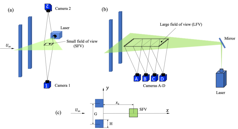
Figure 1: (a) PIV set-up for the energy dissipation rate measurements. (b) PIV set-up for the integral length scale measurements. (c) The coordinate system normal to the prisms’ spanwise direction and definitions of $G$, $H$ and $x_{c}$. All fields of view in (a), (b) and (c) and laser sheets in (a) and (b) are in the horizontal $(x,y)$ plane. Figure courtesy of Chen et al (2021).

4 The experiment of Chen et al. (2021)

Given that the laboratory experiments of Chen et al. (2021) provided the motivation for the developments in the previous section, it is natural to test the previous section’s theory against data from that experiment. In this section we give a brief reminder of the salient features of the experiment of Chen et al. (2021) (a detailed description can of course be found in their paper) and we describe the data from that experiment which we use in section 5.

Chen et al. (2021) experimented with three different turbulent wakes of two side-by-side identical square prisms of side length/width $H=0.03$m. The three different cases corresponded to three different gap ratios $G/H=1.25,2.4,3.5$ chosen because they give rise to three qualitatively different flow regimes in terms of dynamics, large-scale features and inhomogeneity. $G$ is the centre-to-centre distance between the prisms (see figure 1 reproduced here from Chen et al. (2021)). The wind tunnel’s test section was 2m wide by 1m high and the prisms were placed with their spanwise axis parallel to the tunnel’s height. Chen et al. (2021) acquired data for three incoming velocities $U_{\infty}=5,6,7.35$ m/s corresponding to global Reynolds numbers $Re$ $(\equiv U_{\infty}H/\nu)$ = 1.0, 1.2 and $1.5\times 10^{4}$, respectively.

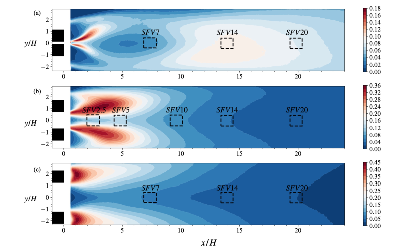
Figure 2: Spatial distributions of the normalised turbulent kinetic energy $k/U_{\infty}^{2}$ at Re = $1.0\times 10^{4}$ and the positions of the small fields of view (dashed squares) for each gap ratio. (a) G/H = 1.25, (b) 2.4, and (c) 3.5. Figure courtesy of Chen et al. (2021).

Two different 2D2C PIV set-ups were used, one designed for turbulent dissipation measurements (see figure 1a) and the other for measurements of integral length scale (see figure 1b), both measuring two horizontal fluid velocity components in the horizontal $(x,y)$ plane normal to the vertical span of the prisms. A dual-camera PIV system with small field of view (SFV) was used for the turbulent kinetic energy dissipation rate (see figure 1a, c). Two sCMOS cameras, one over the top and one under the bottom of the test section, observed the same SFV and obtained two independent measurements of the same velocity fields which were then used to reduce the noise in estimating the energy dissipation rate (see Chen et al. (2021) for detailed explanations). The SFV size was similar to the horizontal size of the prisms, specifically about 1$H$ in streamwise direction by 0.9$H$ in cross-stream direction (figure 1a, c).

Table 1: Details of the small fields of view (SFV).

$Re$		$1.0\times 10^{4}$				$1.2\times 10^{4}$				$1.5\times 10^{4}$
$G/H$		1.25	2.4	3.5		1.25	2.4	3.5		3.5
Cases		SFV7	SFV2.5	SFV7		SFV14	SFV14	SFV14		SFV20
		SFV14	SFV5	SFV14		SFV20	SFV20	SFV20
		SFV20	SFV10	SFV20
			SFV20

For each gap ratio $G/H$, Chen et al. (2021) took measurements with SFVs at several downstream positions for two or three global Reynolds numbers $Re$. The centre of all the SFVs was on the geometric centerline ($y=0$), as sketched in figure 1c, and different SFVs differed by different streamwise positions $x_{c}$ of the SFV centre. The measurement cases are summarized in table 1. The different SFVs are referred to as SFV$\mathcal{N}$ where $\mathcal{N}$ gives an idea in terms of multiples $\mathcal{N}$ of $H$ of the approximate streamwise coordinate $x_{c}$ of the centre of the SFV. The positions of the SFVs relative to the prisms can be seen in figure 2. In this study we use data from all the cases listed in table 1 except $G/H=1.25$ and $3.5$ at the smallest Reynolds number ($1.0\times 10^{4}$).

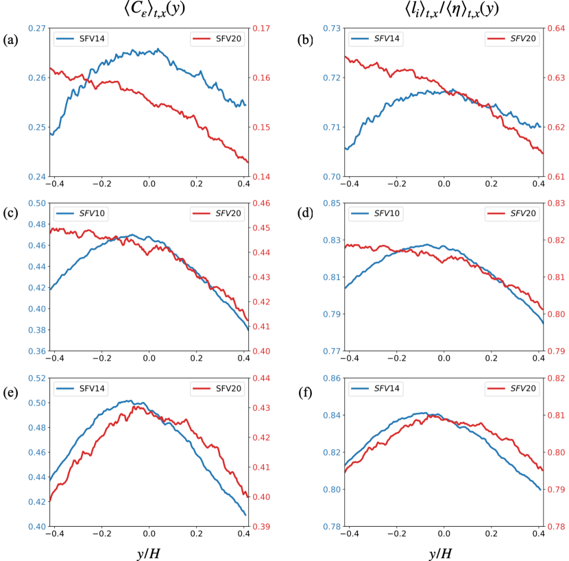
Figure 3: Left plots (a, c, e) show $\langle C_{\varepsilon}\rangle_{t,x}$, where the brackets $\langle...\rangle_{t,x}$ signify an average over time $t$ and streamwise coordinate $x$, versus $y/H$ within a small field of view. The right plots (b, d, f) show $\langle l_{i}\rangle_{t,x}/\langle\eta\rangle_{t,x}$ versus $y/H$, where $l_{i}=LR^{-3/4}$ and $\eta=(\nu^{3}/\langle\varepsilon\rangle)^{1/4}$. Red lines correspond to SFV20 and blue lines to SFV14 (a, b, e, f) or SFV10 (c, d). $Re=1.0\times 10^{4}$. Plots (a, b) are for $G/H=1.25$; (c, d) for $G/H=2.4$; (e, f) for $G/H=3.5$.

The other 2D2C PIV set-up used by Chen et al. (2021) was a system of four sCMOS cameras arranged consecutively in streamwise direction to allow integral length scale measurements in a large field of view (LFV) ranging from $x=0.53H$ to $x=24.3H$ in streamwise direction and $y=-2.4H$ to $y=2.9H$ in cross-stream direction for $Re=1.0\times 10^{4}$, and from $x=11.1H$ to $x=24.9H$ and $y=-2.8H$ to $y=3H$ for $Re=1.2$ and $1.5\times 10^{4}$, see figure 1b.

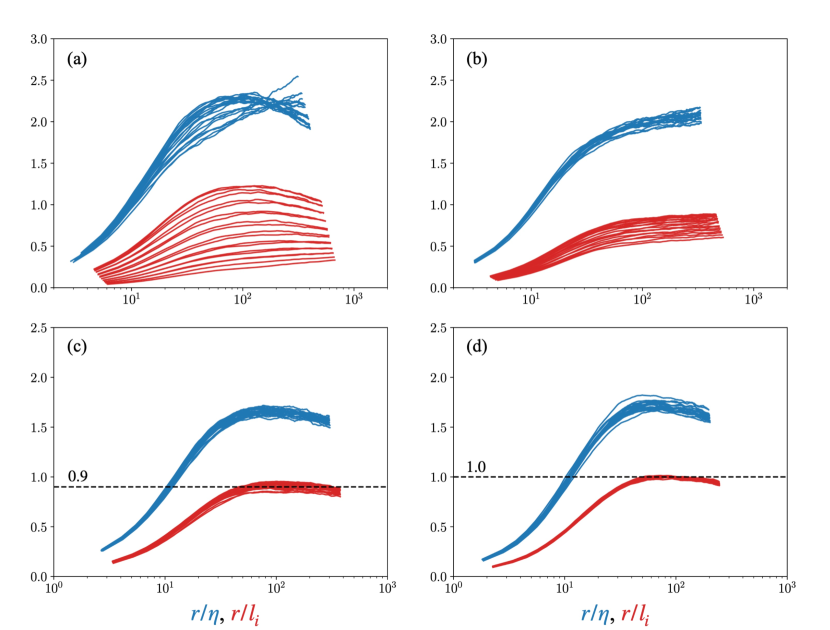
Figure 4: Comparison between $S_{2}^{u}/(\langle\varepsilon\rangle r)^{2/3}$ (blue, $r/\eta$ in abscissa where $\eta=(\nu^{3}/\langle\varepsilon\rangle)^{1/4}$) and $S_{2}^{u}/(k^{3/2}r/L)^{2/3}$ (red, $r/l_{i}$ in abscissa where $l_{i}=LR^{-3/4}$, $R=\sqrt{k}L/\nu$) across the flow (different same-colour curves are for different values of $y$) in each SFV for G/H = 2.4 at $Re=1.0\times 10^{4}$. (a) SFV2.5, (b) SFV5, (c) SFV10, (d) SFV20.

The acquisition frequency was 5Hz for SFV and 4Hz for LFV. 20,000 velocity fields were captured for each measurement, corresponding to about 67 mins for SFV measurements and 83mins for LFV measurements. The final interrogation window size of their PIV analysis was $24\times 24$ pixels with about $58\%$ overlap, which correspond to a $312\mu m$ interrogation window for SFV and 1.6mm for LFV. In the SFVs, the ratio of the interrogation window size to the Kolmogorov length scale varied from 4.5 at the nearest position (SFV2.5) to 2.5 at the farthest position (SFV20), and was below 3.2 for $x/H>10$ (see figure 2 in Chen et al. (2021)). The turbulent energy dissipation rate was approximated based on the assumption of local axisymmetry in the streamwise direction (George & Hussein, 1991). Lefeuvre et al. (2014) demonstrated that the turbulent kinetic energy dissipation rate estimated based on this assumption is a good representation of the full energy dissipation rate across the stream in the wake of a square prism, in fact more accurate than the turbulent energy dissipation rate estimated from the local isotropy assumption.

The turbulent kinetic energy $k$ was estimated from the two horizontal turbulent velocity components and showed, using direct numerical simulation data from Zhou et al. (2019), that the ratio of this estimate to the full turbulent kinetic energy remains about constant at 0.75 to 0.8 for streamwise distances $x/H\geq 5$. They also calculated correlation length scales in the streamwise direction of both streamwise and cross-stream fluctuating velocities. Good convergence of the auto-correlation functions was achieved for the cross-stream fluctuations whereas the streamwise fluctuations gave rise to integral length scales close to $10H$ in those cases when it was possible to extract values of this length scale from the auto-correlation function (the auto-correlation function of streamwise velocity fluctuations often did not converge to $0$). We therefore adopt their choice of integral length-scale $L$ which is the integral length scale of the cross-stream turbulence fluctuations in the streamwise direction. We use their data for $L$ in the following cases: $G/H=1.25$, $SFV14$ and $SFV20$, where $L/H$ ranges from about $1.4$ to $1.6$; $G/H=2.4$ where $L/H$ ranges between $0.4$ and $0.5$ in SFV2.5, $0.75$ to $0.8$ in SFV5, and hovers around 1 in SFV14 and SFV20; and $G/H=3.5$, SFV14 and SFV20, where $L/H$ ranges between about 1/2 and about 2/3.

In section 5 we use the integral length scale data just mentioned and also local streamwise and cross-stream velocity data obtained by Chen et al. (2021) in SFVs as well as local turbulent dissipation rate $\varepsilon$ and local turbulent kinetic energy data in SFVs.

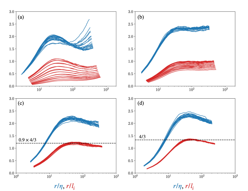
Figure 5: Comparison between $S_{2}^{v}/(\langle\varepsilon\rangle r)^{2/3}$ (blue, $r/\eta$ in abscissa where $\eta=(\nu^{3}/\langle\varepsilon\rangle)^{1/4}$)) and $S_{2}^{u}/(k^{3/2}r/L)^{2/3}$ (red, $r/l_{i}$ in abscissa where $l_{i}=LR^{-3/4}$, $R=\sqrt{k}L/\nu$) across the flow (different same-colour curves are for different values of $y$) in each SFV for G/H = 2.4 at $Re=1.0\times 10^{4}$. (a) SFV2.5, (b) SFV5, (c) SFV10, (d) SFV20.

5 Scalings of second order structure functions

In this section, we assess our theory’s prediction (36) for the longitudinal structure function as well as the equivalent prediction for the transverse structure function in the three turbulent wake flows described in the previous section.

Figure 2 shows the spatial distribution of the turbulent kinetic energy in the three flows and illustrates the qualitative differences between them. Each flow represents one of the three different flow regimes obtained for different values of $G/H$ (see Sumner et al., 1999; Alam et al., 2011): the ‘single-bluff-body regime’ (G/H = 1.25), the ‘bistable regime’ (G/H = 2.4) and the ‘coupled vortex regime’ (G/H = 3.5). Consistently, the turbulent kinetic energy field, as well as the mean flow and integral scale fields (not reproduced here from Chen et al. (2021)), exhibit distinct spatial distributions and different inhomogeneity structures which are described and discussed in Chen et al. (2021). The inhomogeneity is also present within the SFVs where the turbulence dissipation coefficient $C_{\varepsilon}$ is found to vary significantly and systematically with spatial position in different SFVs (see figure 3) in ways that are common in the three different flows, even though the spatial inhomogeneities of turbulent kinetic energy and the turbulence dissipation rate vary from flow to flow (see figure 18 in Chen et al. (2021)). These qualitative differences in large-scale features and inhomogeneity provide some variety for the testing of the predictions of section 3.

We use the data of Chen et al. (2021) to calculate the longitudinal structure function $S_{2}^{u}\equiv<[u^{\prime}_{1}(x_{0}+r,y)-u^{\prime}_{1}(x_{0},y)]^{2}>$ and the transverse structure function $S_{2}^{v}\equiv<[u^{\prime}_{2}(x_{0}+r,y)-u^{\prime}_{2}(x_{0},y)]^{2}>$ where use is made of the Reynolds decomposition $u_{1}=U_{1}+u^{\prime}_{1}$ and $u_{2}=U_{2}+u^{\prime}_{2}$ into mean flow components $U_{1}$ (streamwise) and $U_{2}$ (cross-stream) and turbulent fluctuating velocity components $u^{\prime}_{1}$ and $u^{\prime}_{2}$. The averaging operation is over 20,000 velocity field snapshots and we checked that there is no significant dependence on the choice of streamwise origin $x_{0}$ for all the $G/H$, $SFV$ and $Re$ cases examined here, except perhaps $G/H=2.4$ at $SFV2.5$, where changes of $x_{0}$ can create slight shifts of the curves in figures 4a and 5a without significantly changing their shape.

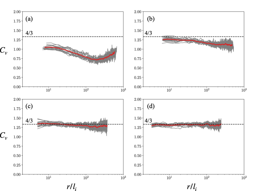
Figure 6: $C_{v}(r/l_{i})$ versus $r/l_{i}$ (where $l_{i}=LR^{-3/4}$ with $R=\sqrt{k}L/\nu$) for $G/H=2.4$ and $Re=1.0\times 10^{4}$ at (a) SFV2.5, (b) SFV5, (c) SFV10 and (d) SFV20. The horizontal dashed line is $C_{v}=4/3$. Different lines correspond to different $y$ and the red line is the average curve.

The theory of section 3 was presented for the longitudinal and transverse structure functions involving $u_{1}$ and $u_{2}$ rather than $u^{\prime}_{1}$ and $u^{\prime}_{2}$. In fact, these structure functions are insensitive to this difference in all the plots presented in figures 4 to 13 except for two: the plot in figure 4a which corresponds to the very near field SFV2.5 where the streamwise mean flow varies appreciably in both the streamwise and the cross-stream directions within the SFV; and, very slightly, the plot in figure 8a which is another case where the streamwise mean flow varies appreciably in the streamwise direction within the SFV (though less in the cross-stream direction in this case).

We start the presentation and discussion of our data analysis with figures 4 and 5 where we plot normalised $S_{2}^{u}$ and $S_{2}^{v}$, respectively, as functions of normalised $r$ for different cross-stream coordinates $y$ in the case $G/H=2.4$, $Re=10^{4}$. This is the case for which we have data from four different SFV stations and therefore can get an impression of dependence on streamwise distance from the pair of square prisms. Neither the Kolmogorov scalings $S_{2}^{u}/(\varepsilon r)^{2/3}$ and $S_{2}^{v}/(\varepsilon r)^{2/3}$ versus $r/\eta$ (which we show for comparison even though they should not be expected to hold in locally non-homogeneous turbulence) nor our scaling (36), i.e. $S_{2}^{u}/k(r/L)^{2/3}$ and $S_{2}^{v}/k(r/L)^{2/3}$ versus $r/l_{i}$, collapse the data well in the SFV stations closest to the prisms, i.e. SFV2.5 and SFV5. However, our scaling returns a clearly better collapse than Kolmogorov’s in SFV20 and the two different types of scaling may be judged as comparable, perhaps with a slight preference for scaling (36), in SFV10.

It is intriguing that the curves $S_{2}^{v}/k(r/L)^{2/3}$ versus $r/l_{i}$ appear to plateau at a value that is about $4/3$ the value where the curves $S_{2}^{u}/k(r/L)^{2/3}$ versus $r/l_{i}$ appear to plateau in SFV10 and SFV20 (see figures 4(c, d) and 5(c, d)). The presence of such a $4/3$ multiplier is well understood in cases where the turbulence is isotropic and locally homogeneous, in which cases it is possible to prove the relation $S_{2}^{v}=S_{2}^{u}+{r\over 2}{\partial S_{2}^{u}\over\partial r}$ (e.g. see Pope, 2000). Indeed, if $S_{2}^{u}=A_{u}r^{2/3}$ in a certain range of scales, then $S_{2}^{v}=S_{2}^{u}+{r\over 2}{\partial S_{2}^{u}\over\partial r}$ implies $S_{2}^{v}={4\over 3}A_{u}r^{2/3}$ in that same range of scales. There is no local homogeneity in any SFV studied here given that the turbulence is inhomogeneous within them and that their size is comparable to the local integral length-scales (between under 1/2 to slightly over 3/2 the integral scale $L$). The usual way to derive $S_{2}^{v}=S_{2}^{u}+{r\over 2}{\partial S_{2}^{u}\over\partial r}$ can therefore not be applied here. Nevertheless, our theory’s inner scaling predictions $S_{2}^{u}=k(r/L)^{2/3}f_{u}(r/l_{i})$ and $S_{2}^{v}=k(r/L)^{2/3}f_{v}(r/l_{i})$, if injected in $S_{2}^{v}=S_{2}^{u}+{r\over 2}{\partial S_{2}^{u}\over\partial r}$, yield $f_{v}={4\over 3}f_{u}+{(r/l_{i})\over 2}{\partial f_{u}\over\partial(r/l_{i})}$, which means that $C_{v}$ defined as follows should equal $4/3$, i.e.

$$C_{v}\equiv{f_{v}-{(r/l_{i})\over 2}{\partial f_{u}\over\partial(r/l_{i})}\over f_{u}}=4/3.$$ (38)

Note that the value $4/3=1+(2/3)/2$ results from the exponent $2/3$. If $C_{v}$ differs from $4/3$ then either our theory’s predictions are at fault or $S_{2}^{v}=S_{2}^{u}+{r\over 2}{\partial S_{2}^{u}\over\partial r}$ does not hold or both.

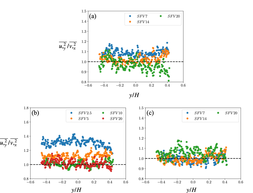
Figure 7: $\langle u,_{y}^{2}\rangle/\langle v,_{x}^{2}\rangle$ versus normalised cross-stream coordinate $y/H$ in different SFVs for $Re=1.0\times 10^{4}$ and (a) $G/H=1.25,(b)2.4,(c)3.5$.

In figure 6 we plot $C_{v}$ versus $r/l_{i}$ obtained from the previous two figures for $G/H=2.5$, $Re=10^{4}$. $C_{v}$ is clearly well below $4/3$ at all scales in SFV2.5 where the departure from collapse of $S_{2}^{u}$ and $S_{2}^{v}$ for different values of $y$ is the greatest. However, $C_{v}$ tends to $4/3$ gradually from below as the SFV moves further away from the prisms, and at SFV20 one can say that $C_{v}$ is close to $4/3$ for all values of $y$ over the entire range of $r/l_{i}$. This is a non-trivial observation which will require future investigation because Chen et al. (2021) showed quite clearly that there is no local homogeneity in SFV20 in terms of turbulent kinetic energy and turbulent dissipation rate, which means that the usual grounds for $S_{2}^{v}=S_{2}^{u}+{r\over 2}{\partial S_{2}^{u}\over\partial r}$ are absent even though the mean flow may be at its closest to local homogeneity in SFV20 compared to other SFV stations. At this stage, we have no explanation for this result but we do note that it is consistent with the theory’s 2/3 exponent prediction for the second order structure functions’ power law behaviour in the intermediate range of scales. Figures 4(c, d) and 5(c, d) may be giving some partial support to this 2/3 exponent in SFV10 and SFV20 but over a range of scales that is much smaller than the range of scales where $C_{v}$ effectively equals $4/3$ in SFV20 and where $C_{v}$ is close to $4/3$ in SFV10.

Figure 8: Comparison between $S_{2}^{u}/(\langle\varepsilon\rangle r)^{2/3}$ (blue, $r/\eta$ in abscissa where $\eta=(\nu^{3}/\langle\varepsilon\rangle)^{1/4}$) and $S_{2}^{u}/(k^{3/2}r/L)^{2/3}$ (red, $r/l_{i}$ in abscissa where $l_{i}=LR^{-3/4}$, $R=\sqrt{k}L/\nu$) across the SFV14 and SFV20 for all gap ratios at $Re=1.2\times 10^{4}$. Different same-colour curves correspond to different $y$ positions. (a) $G/H=1.25$, SFV14, (b) $G/H=1.25$, SFV20; (c) $G/H=2.4$, SFV14, (d) $G/H=2.4$, SFV20; (e) $G/H=3.5$, SFV14, (f) $G/H=3.5$, SFV20.

It may be that $C_{v}$ is actually more sensitive to anisotropy than inhomogeneity. We therefore conducted a local isotropy test, reported in figure 7, where we examined the ratio $\langle u,_{y}^{2}\rangle/\langle v,_{x}^{2}\rangle$ ($u,_{y}\equiv\partial u^{\prime}_{1}/\partial y$ and $v,_{x}\equiv\partial u^{\prime}_{2}/\partial x$) across the stream (different $y$-positions) in each SFV for different values of $G/H$. This ratio was taken at the same $x_{0}$ (at a distance of about $H/10$ from the upstream edge of each SFV) where the structure functions reported in this paper have been calculated, but we checked that figure 7 does not depend significantly on $x_{0}$. Departures from $\langle u,_{y}^{2}\rangle/\langle v,_{x}^{2}\rangle=1$ indicate departures from local isotropy and the biggest such departures are found at SFV2.5 followed by SFV5 (see figure 7b). The case SFV2.5, $G/H=2.4$ is indeed the case where our second order structure functions are furthest from collapse, whether in Kolmogorov variables or along the lines of our scaling (36) (see figures 4a and 5a). There is also unsatisfactory collapse in SFV5 (see figures 4b and 5b), and figure $\ref{fig:isotropy test}b$ shows that a significant departure from local isotropy remains there. In fact, figure 7 suggests that $\langle u,_{y}^{2}\rangle/\langle v,_{x}^{2}\rangle$ takes values closest to 1 (with a tolerance of about 10%), and therefore does not indicate significant departures from local isotropy, further downstream, beyond SFV7 for all three $G/H$ values. Given that figures 6 and 7 suggest that isotropy may be a prerequisite for our theory’s scalings to hold, a point which will also require future investigation given that isotropy did not feature explicitly in our theory’s assumptions, we limit the remainder of our data analysis to SFV14 and SFV20 in all three $G/H$ cases (Chen et al. (2021) did not take SFV10 measurements for $G/H=1.25$ and $G/H=3.5$). The data for these SFV stations come with values of $Re$ higher than $10^{4}$ which is welcome given that our theory has been developed for high Reynolds numbers.

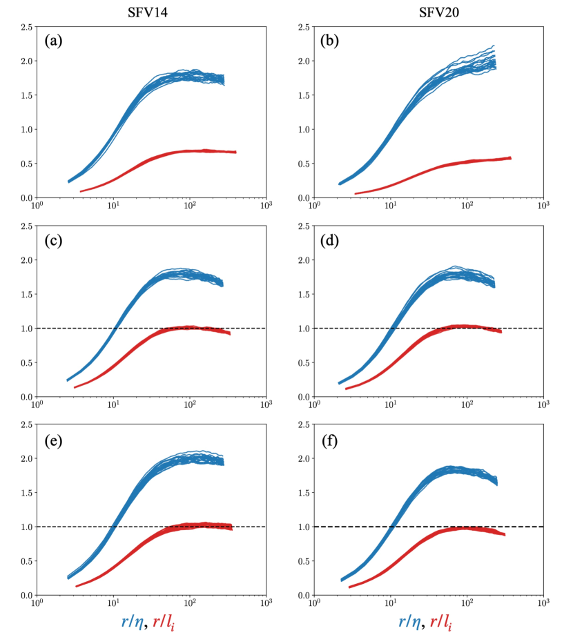
Figure 9: Comparison between $S_{2}^{v}/(\langle\varepsilon\rangle r)^{2/3}$ (blue, $r/\eta$ in abscissa where $\eta=(\nu^{3}/\langle\varepsilon\rangle)^{1/4}$) and $S_{2}^{v}/(k^{3/2}r/L)^{2/3}$ (red, $r/l_{i}$ in abscissa where $l_{i}=LR^{-3/4}$, $R=\sqrt{k}L/\nu$) across the SFV14 and SFV20 for all gap ratios at $Re=1.2\times 10^{4}$. Different same-colour curves correspond to different $y$ positions. (a) $G/H=1.25$, SFV14, (b) $G/H=1.25$, SFV20; (c) $G/H=2.4$, SFV14, (d) $G/H=2.4$, SFV20; (e) $G/H=3.5$, SFV14, (f) $G/H=3.5$, SFV20.

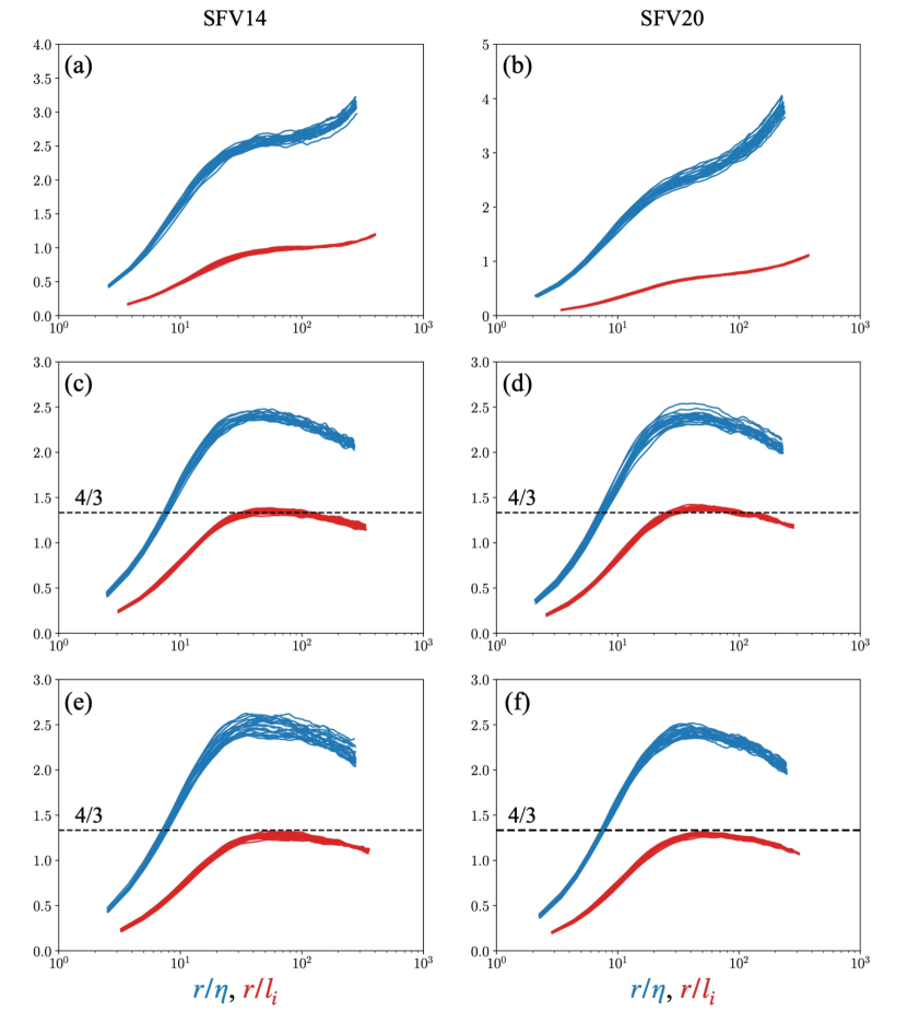
Figure 10: $C_{v}(r/l_{i})$ versus $r/l_{i}$ (where $l_{i}=LR^{-3/4}$ with $R=\sqrt{k}L/\nu$) for SFV14 and SFV20 at $Re=1.2\times 10^{4}$ for all $G/H$ values. Different curves correspond to different $y$-positions and the red line is the average curve. The horizontal dashed line in all the plots indicates the value $4/3$. (a) $G/H=1.25$, SFV14; (b) $G/H=1.25$, SFV20; (c) $G/H=2.4$, SFV14$;(d)$G/H=2.4$,SFV20;(e)$G/H=3.5$,SFV14$; (f) $G/H=3.5$, SFV20.

In figures 8 and 9 we plot, respectively, normalised $S_{2}^{u}$ and $S_{2}^{v}$ as functions of normalised $r$ for different cross-stream coordinates $y$ and all three gap ratios, in SFV14 and SFV20 at $Re=12,000$. Our scaling (36), i.e. $S_{2}^{u}/k(r/L)^{2/3}$ and $S_{2}^{v}/k(r/L)^{2/3}$ versus $r/l_{i}$, collapses the data well in both SFV stations and for all three gap ratios. The Kolmogorov scalings $S_{2}^{u}/(\varepsilon r)^{2/3}$ and $S_{2}^{v}/(\varepsilon r)^{2/3}$ versus $r/\eta$ (which we show for comparison even though they should not be expected to hold here) returns a much worse collapse in all cases. There is a general tendency towards a plateau in $S_{2}^{u}/k(r/L)^{2/3}$ for $r/l_{i}\geq 40$ which supports the theory’s intermediate range $r^{2/3}$ prediction for the $r$-dependence of $S_{2}$. However, there is also a difference between $G/H=1.25$ and the other two $G/H$ values which is most notable in figure 9: the normalised $S_{2}^{v}$ takes a turn towards higher values as $r/l_{i}$ increases beyond about 90 in the $G/H=1.25$ case but not in the other two cases. Consistently with this observation, $C_{v}$ is also qualitatively different for $G/H=1.25$ and for the two other values of $G/H$ (see figure 10): it takes values significantly above $4/3$ and in fact increasing with increasing $r$ for $r/l_{i}$ larger than about $100$ in the $G/H=1.25$ case, whereas nothing of the sort happens in the two other $G/H$ cases. In fact, $C_{v}$ is very close to $4/3$ for all $y$ and all $r/l_{i}$ sampled at SFV20 for both $G/H=$ $2.4$ and $3.5$. The same is the case at SFV14 for $G/H=2.4$ but slightly less so for $G/H=3.5$ where $C_{v}$ is close to $4/3$ for $r/l_{i}$ below about 40 and slightly decreases gradually below $4/3$ with increasing $r/l_{i}$ beyond $r/l_{i}=40$. We note once again that the close to $4/3$ values of $C_{v}$ may signify indirect support of the $2/3$ exponent in the power-law dependence on $r$ of the second order structure functions. A range with such a power law is more visible, though, in $S_{2}^{u}$ (figure 8) than $S_{2}^{v}$ (figure 9).

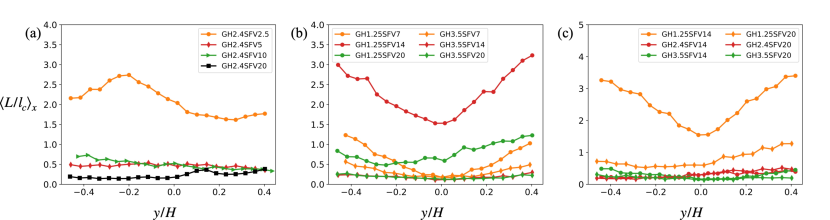
Figure 11: Cross-stream profiles (along $y$ within an SFV) of $\langle L/l_{c}\rangle_{x}$, where $\langle\cdot\rangle_{x}$ denotes streamwise averaging within the SFV. (a) $G/H=2.4$, $Re=1.0\times 10^{4}$, (b) $G/H=1.25$ and $3.5$, $Re=1.0\times 10^{4}$. (c) $G/H=1.25$, $2.4$ and $3.5$, $Re=1.2\times 10^{4}$.

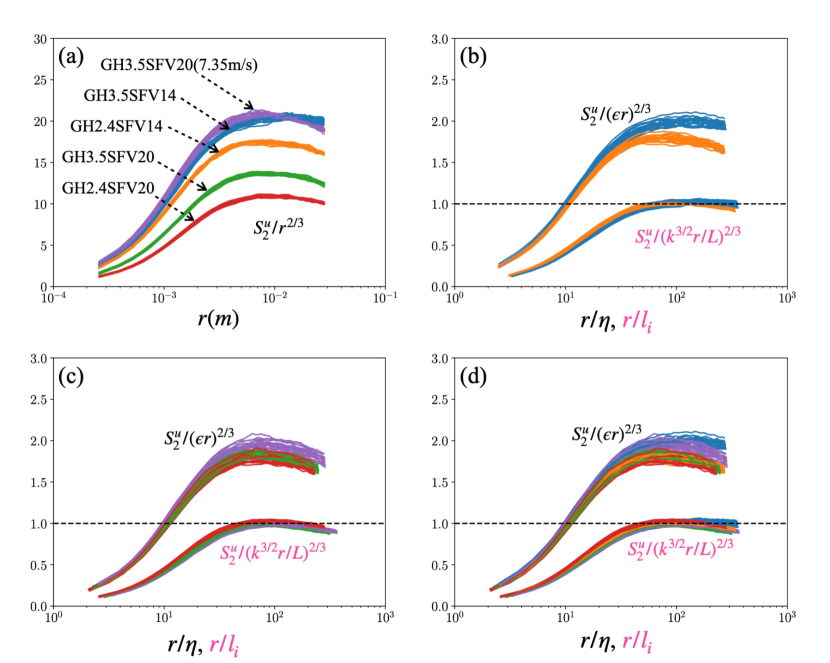
Figure 12: (a) $S_{2}^{u}/r^{2/3}$ versus $r$ for 5 different cases: (i) SFV14, $G/H=2.4$, $Re=1.2\times 10^{4}$; (ii) SFV14, $G/H=3.5$, $Re=1.2\times 10^{4}$; (iii) SFV20, $G/H=2.4$, $Re=1.2\times 10^{4}$; (iv) SFV20, $G/H=3.5$, $Re=1.2\times 10^{4}$; (v) SFV20, $G/H=3.5$, $R=1.5\times 10^{4}$. Different same-colour curves correspond to different $y$ positions. (b) $S_{2}^{u}/(k^{3/2}r/L)^{2/3}$ versus $r/l_{i}$ (where $l_{i}=LR^{-3/4}$ with $R=\sqrt{k}L/\nu$) and $S_{2}^{u}/(\langle\varepsilon\rangle r)^{2/3}$ versus $r/\eta$ (where $\eta=(\nu^{3}/\langle\varepsilon\rangle)^{1/4}$) for cases (i) and (ii), i.e. SFV14. (c) Same as (b) but for cases (iii), (iv) and (v), i.e. SFV20. (d) Same as (b) and (c) but for all cases, SFV14 and SFV20.

The departures of $C_{v}$ from $4/3$ in the near field positions SFV2.5 and SFV5 of the $G/H=2.4$ flow (figure 6) could be accounted for by the departures from local isotropy evidenced in figure 7. However, the departures of $C_{v}$ from $4/3$ seen in figure 10 for the $G/H=1.25$ flow case cannot be explained that way (see figure 7). We therefore investigate the possibility that mean shear may be responsible for these departures. We estimate a Corrsin length $l_{C}\equiv\sqrt{\langle\epsilon\rangle/S^{3}}$ (see Sagaut & Cambon (2018)), following Kaneda (2020), and compare it to our estimate of the integral length-scale $L$ (see penultimate paragraph of section 4). In figure 11 we plot $\langle L/l_{C}\rangle_{x}$ as a function of cross-stream coordinate $y$ where $\langle\cdot\rangle_{x}$ symbolises averaging over streamwise coordinate $x$ within a small field of view (SFV) and where $l_{C}$ is calculated by taking $S=|{\partial U_{1}\over\partial x}|+|{\partial U_{1}\over\partial y}|+|{\partial U_{2}\over\partial x}|+|{\partial U_{2}\over\partial y}|$ to avoid over-estimating $l_{C}$. For SFV14 and SFV20 in the flow cases $G/H=2.4$ and $3.5$ where our theory agrees well with the experimental data, $\langle L/l_{C}\rangle_{x}$ is well below $0.5$, suggesting that mean shear is absent at the length-scales considered for the second order structure functions. This agrees with our observation in this section’s fourth paragraph that these structure functions are effectively the same at $SFV14$ and $SFV20$ for $G/H=2.4$ and $3.5$ if calculated for the instantaneous or the fluctuating velocities. Consistently perhaps, $\langle L/l_{C}\rangle_{x}$ is larger than $1.5$ for SFV2.5, $G/H=2.4$ where neither Kolmogorov’s nor our scalings work (figures 4 and 5). Turbulence production and anisotropy should be taken somehow explicitely into account in this case, which the theory in section 3 does not. Such an extension of our theory may also be needed for SFV5, $G/H=2.4$ where our theory’s scalings also do not work well (figures 4 and 5) and $\langle L/l_{C}\rangle_{x}$ takes values up to about 0.75.

However, $\langle L/l_{C}\rangle_{x}$ cannot be, on its own, a reliable criterion for the applicability of the theory in section 3. It takes values at SFV10, $G/H=2.4$ which are comparable to those that it takes at SFV5, $G/H=2.4$, yet our theory’s collapse for the second order structure functions is not as bad at SFV10 as it is at SFV5 (see figures 4 and 5). More dramatically, $\langle L/l_{C}\rangle_{x}$ is larger than 1.5 at SFV14 in the $G/H=1.25$ flow case, yet the collapse there is good (figures 8a and 9a) with the only exception that the exponent $2/3$ may not be present in $S_{2}^{v}$. At SFV20 in the same flow, $\langle L/l_{C}\rangle_{x}$ takes values between $0.5$ and $1.1$, larger than the values it takes at SFV14 and SFV20 for $G/H=2.4$ and $3.5$ where the theory works rather well (figures 8 and 9), but well below $1.5$, the smallest value it takes at SFV14 for $G/H=1.25$. Yet, at SFV20 of this $G/H=1.25$ flow, the exponent $2/3$ appears absent from both $S_{2}^{u}$ and $S_{2}^{v}$ even though our scalings collapse them both very well. Also, $C_{v}$ is similar at SFV14 and SFV20 of this flow case (figures 10a, b). All in all, we cannot quite conclude that the Corrsin length $l_{C}$ can be used on its own as the basis for an applicability criterion of our theory (e.g. that the theory appplies where $\langle L/l_{C}\rangle_{x}$ is smaller than 0.5 but does not apply where it is larger than 1). Clearly, the determination of the range and criteria of applicability of the theory requires more research which we must leave for future studies.

We now go one step further and explore the possibility that the scaling (36) may be able to collapse second order structure functions across flows (i.e. different values of $G/H$), at different streamwise stations in these flows and for different Reynolds numbers. Even though we consider only two different SFV stations (SFV14 and SFV20), only two Reynolds numbers ($Re=12,000$ and $15,000$, see table 1) and only two of our three flows ($G/H=2.4$ and $3.5$), it does remain worthwhile to test for such collapse. The $G/H=1.25$ flow case is not included in this test because of the clear differences between $G/H=1.25$ on the one hand and $G/H=2.4$, $3.5$ on the other hand which are evidenced in figures 8 and 9.

In figures 12a and 13a we plot, respectively, $S_{2}^{u}/r^{2/3}$ and $S_{2}^{v}/r^{2/3}$ versus $r$ (in meters) for a wide range of $y$ positions (within the SFV) and five different cases: (i) SFV14, $G/H=2.4$, $Re=12,000$; (ii) SFV14, $G/H=3.5$, $Re=12,000$; (iii) SFV20, $G/H=2.4$, $Re=12,000$; (iv) SFV20, $G/H=3.5$, $Re=12,000$; (v) SFV20, $G/H=3.5$, $R=15,000$. There is no collapse. As a second step, we plot in figures 12b and 13b, $S_{2}^{u}/(k^{3/2}r/L)^{2/3}$ and $S_{2}^{v}/(k^{3/2}r/L)^{2/3}$ respectively, both versus $r/l_{i}$, for cases (i) and (ii) which are for SFV14. The collapse is defensible but better for $S_{2}^{u}$ than for $S_{2}^{v}$. These two structure functions are also plotted with Kolmogorov scalings in these two figures for comparison and it is clear that the Kolmogorov scalings cannot achieve collapse, particularly for $S_{2}^{u}$. Our third step is to test for collapse in SFV20. For this, we plot $S_{2}^{u}/(k^{3/2}r/L)^{2/3}$ and $S_{2}^{v}/(k^{3/2}r/L)^{2/3}$ versus $r/l_{i}$ for cases (iii), (iv) and (v) which are for SFV20 (see figures 12c and 13c). Conclusions are similar. In a final step, we plot all cases (i), (ii), (iii), (iv) and (v) together in figures 12d and 13d. There is a defensible collapse for $S_{2}^{u}$ across these two flows, two flow stations, and two Reynolds numbers, much better than if a collapse was attempted in Kolmogorov variables. One may say that there is also a more or less acceptable collapse for $S_{2}^{v}$, but it is less sharp than the collapse of $S_{2}^{u}$. However, a careful look at the plots, in particular figures 13 (b, c), reveals that there remains some dependence on $G/H$ at SFV14 and SFV20, i.e. some dependence of the similarity function $f_{v}(r/l_{i},G/H)$ on inlet conditions at these stations.

6 Conclusions and new research directions

We developed a theory of non-homogeneous turbulence which we applied to free turbulent shear flows. The theory predicts that second order structure functions scale according to equation (36) in non-homogeneous turbulence, i.e.

$$S_{2}^{u}=k(r/L)^{2/3}f_{u}(r/l_{i})$$ (39)

and

$$S_{2}^{v}=k(r/L)^{2/3}f_{v}(r/l_{i})$$ (40)

where $l_{i}$ is an inner length-scale which differs from but has the same dependence on viscosity as the Kolmogorov length-scale $\eta$. These scalings take non-homogeneity explicitely into account and are different from Kolmogorov scalings. However they become identical to Kolmogorov scalings in homogeneous stationary turbulence. Note that the theory also leads to the intermediate range proportionality (37) irrespective of the presence of inhomogeneity-related energy transfer mechanisms.

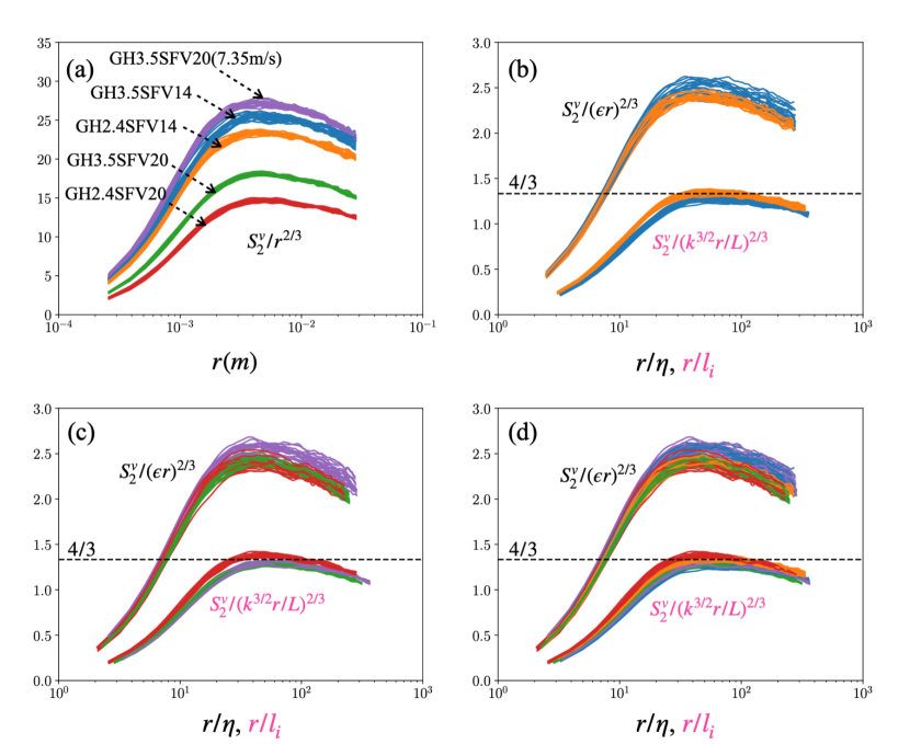
Figure 13: (a) $S_{2}^{v}/r^{2/3}$ versus $r$ for 5 different cases: (i) SFV14, $G/H=2.4$, $Re=1.2\times 10^{4}$; (ii) SFV14, $G/H=3.5$, $Re=1.2\times 10^{4}$; (iii) SFV20, $G/H=2.4$, $Re=1.2\times 10^{4}$; (iv) SFV20, $G/H=3.5$, $Re=1.2\times 10^{4}$; (v) SFV20, $G/H=3.5$, $R=1.5\times 10^{4}$. Different same-colour curves correspond to different $y$ positions. (b) $S_{2}^{v}/(k^{3/2}r/L)^{2/3}$ versus $r/l_{i}$ (where $l_{i}=LR^{-3/4}$ with $R=\sqrt{k}L/\nu$) and $S_{2}^{v}/(\langle\varepsilon\rangle r)^{2/3}$ versus $r/\eta$ (where $\eta=(\nu^{3}/\langle\varepsilon\rangle)^{1/4}$) for cases (i) and (ii), i.e. SFV14. (c) Same as (b) but for cases (iii), (iv) and (v), i.e. SFV20. (d) Same as (b) and (c) but for all cases, SFV14 and SFV20.

The theory is based on concepts of inner and outer similarity which are used to characterise the non-homogeneity of two-point statistics and on a new inner-outer dissipation equivalence hypothesis. Future research is required to establish the breadth of applicability of this hypothesis and of such similarity assumptions across a variety of non-homogeneous turbulent flows. Isotropy is not explicitly assumed in the theory, but our analysis of the data of Chen et al. (2021) suggests that it may be required at some level. Turbulence production is not explicitely taken into account either and our data analysis also suggests that the theory requires modifications when production cannot be neglected. These are issues which will need to be addressed in future research along with the question of the particular quantities which may obey similarity at the inner and/or outer level, and those which may not. Another important related issue which also requires future research is the issue of large-scale coherent structures and their effects on or just relations to similarity and non-homogeneity and turbulence interscale/interspace transfers. Are they, for example, responsible for the inner-outer equivalence for turbulence dissipation as a property of the type of non-homogeneity considered here? How general is this inner-outer equivalence? We should start thinking in terms of different classes of non-homogeneity depending, for example, on the degree of significance of turbulence production and on differences in coherent structure dynamics in the presence or absence of turbulence production. Alves Portela et al. (2020) showed that non-homogeneity and coherent structures are in fact key for the proper understanding of interscale turbulence transfers in near-field non-homogeneous turbulent wakes. Future research should probably combine their approach with the present one and investigate these new questions.

The data of Chen et al. (2021) which have been used here to test the theory’s new scalings are from three different turbulent wakes of side-by-side identical square prisms. These three non-homogeneous turbulent flows differ by their gap ratio $G/H$ and represent three qualitatively different flow regimes. Good agreement with the theory’s scalings (39) and (40) has been found in all three flows, but far enough from the prisms where the turbulence is clearly not locally homogeneous but nevertheless exhibits some indications of local isotropy. Whereas the scalings (39) and (40) collapse the structure functions rather well in all three flows at these far enough positions (which are actually not so far as they are only between $10H$ and $20H$), the intermediate $r^{2/3}$ power law predicted by the theory is more clearly supported by the data for $S_{2}^{u}$ than for $S_{2}^{v}$. This may or may not be a Reynolds number effect, which is another issue needing to be addressed in future studies. However, there are also clear qualitative differences between $S_{2}^{v}$ for $G/H=1.25$ and $S_{2}^{v}$ for $G/H=2.4$ and $3.5$ even if (40) collapses both cases. These differences point to a power law for $S_{2}^{v}(r)$ which may be slightly different from $r^{2/3}$ in the $G/H=1.25$ case. Differences of this sort can be exploited in future investigations which could lead to a much deeper understanding of scale-by-scale energy scalings and energy transfers in non-homogeneous turbulent flows.

Finally it is worth mentioning that (39) and (40) are also able to more or less collapse structure functions for different cross-stream positions, two far enough streamwise stations, two flow cases $G/H=2.4$, $3.5$ and two Reynolds numbers (see figures 12 and 13). However, some dependence on inlet conditions remains and one may need to take into account some dependence of the similarity functions, particularly $f_{v}$, on $G/H$.

Acknowledgements We are grateful to the authors of Chen et al. (2021) for their data, in particular Dr. Christophe Cuvier who has been essential in the setting up of their experiment and data collection.

Funding. This work was supported by JCV’s Chair of Excellence CoPreFlo funded by I-SITE-ULNE(grant number R-TALENT-19-001-VASSILICOS); MEL(grant number CONVENTION_219_ESR_06) and Region Hauts de France (grant number 20003862).

Declaration of interests. The authors report no confict of interest.

Appendix A Consistency between the inner scale-by-scale energy balance and the inner similarity hypothesis

Using (20) (which we obtained from the outer scale-by-scale balance in section 3.1) and (24), the high Reynolds number inner scale-by-scale energy balance (23) becomes

$$g_{l}^{-1/2}g_{X}\alpha f_{iX}(r/l_{i})+g_{l}^{-1/2}g_{3}\gamma f_{i3}(r/l_{i})+g_{l}^{-1/2}g_{p}\beta f_{ip}(r/l_{i})=$$

$$-1+C_{\varepsilon}^{-1}{\bf\nabla}^{2}_{r/l_{i}}f_{i2}(r/l_{i})$$ (41)

in terms of the dimensionless proportionality constants $\alpha=(V_{oX}/V_{o2})^{3}/C_{\varepsilon}$, $\beta=(V_{op}/V_{o2})^{3}/C_{\varepsilon}$ and $\gamma=(V_{o3}/V_{o2})^{3}/C_{\varepsilon}$ (some of these constants, though not all, could in principle be zero). Irrespective of which transport/transfer term we keep in this high Reynolds number inner energy budget, i.e. which of $g_{l}^{-1/2}g_{X}$, $g_{l}^{-1/2}g_{3}$ and $g_{l}^{-1/2}g_{p}$ we let tend to zero in the limit $R\to\infty$, we end up with a function of $r/l_{i}$ being equal to $-1+C_{\varepsilon}^{-1}{\bf\nabla}^{2}_{r/l_{i}}f_{i2}(r/l_{i})$ which is possible either if $C_{\varepsilon}$ is constant, i.e. independent of ${\bf X}$, or if ${\bf\nabla}^{2}_{r/l_{i}}f_{i2}(r/l_{i})=0$ which means that the longitudinal second order structure function should be a harmonic function of $r$, which is not realistic. As we want a theory for non-homogeneous turbulence where $C_{\varepsilon}$ depends on ${\bf X}$, we need to modify some of the inner similarity assumptions (14), (15) and/or (16).

Firstly, we keep the interscale turbulence energy transfer in the high Reynolds number inner scale-by-scale energy balance. This requires

$$g_{l}^{-1/2}(R)g_{3}(R)=Const$$ (42)

independent of $R$. Secondly, we take $g_{l}^{-1/2}g_{X}=Const$ and $g_{l}^{-1/2}g_{p}=Const$ to allow for the possibility of both or either of the turbulent transport and the velocity-pressure gradient correlation terms to be present in the high Reynolds number inner scale-by-scale energy balance. (These terms can be made to be absent from this balance by artificially setting $\alpha$ and/or $\beta$ equal to $0$ respectively.) We chose to modify the inner similarity forms of these two terms as they concern statistics which do not only involve two-point velocity differences whereas this is not the case of the interscale transfer rate term which does. Looking at (41), the modification that we are forced to make must ensure that $C_{\varepsilon}(1+\alpha f_{iX}+\gamma f_{i3}+\beta f_{ip})$ is independent of ${\bf X}$ (explicitely). We must therefore replace $f_{iX}$ and $f_{ip}$ in (15) and (16) by the following functions of $r/l_{i}$ and ${\bf X}$:

$$f_{iX}(r/l_{i},{\bf X})={F_{iX}(r/l_{i})\over C_{\varepsilon}({\bf X})}-A-Bf_{i3}(r/l_{i})$$ (43)

$$f_{ip}(r/l_{i},{\bf X})={F_{ip}(r/l_{i})\over C_{\varepsilon}({\bf X})}-C-Df_{i3}(r/l_{i})$$ (44)

where $A$, $B$, $C$ and $D$ are dimensionless constants and $F_{iX}$ and $F_{ip}$ are functions of $r/l_{i}$ only. Note that if the turbulent transport term is not present in the high Reynolds number inner scale-by-scale energy balance then $F_{iX}=0$ and $A=B=0$, and if the velocity-pressure gradient correlation term is not present in that balance then $F_{ip}=0$ and $C=D=0$. All possibilities are therefore covered.

With (43) and (44), the requirement that $C_{\varepsilon}(1+\alpha f_{iX}+\gamma f_{i3}+\beta f_{ip})$ must be independent of ${\bf X}$, and in fact equal to ${\bf\nabla}^{2}_{r/l_{i}}f_{i2}(r/l_{i})$, yields $\gamma=\alpha B+\beta D$, $1=\alpha A+\beta C$ and $\alpha F_{iX}+\beta F_{ip}={\bf\nabla}^{2}_{r/l_{i}}f_{i2}(r/l_{i})$. Taking into account (14), (15), (16) and (17), this latter equation represents the following high Reynolds number balance for $r\ll l_{o}$:

$${\bf\nabla}_{X}\cdot\langle{\bf u}_{X}^{\prime}(\delta u_{1})^{2}\rangle+{\bf\nabla}_{r}\cdot\langle\delta{\bf u}(\delta u_{1})^{2}\rangle+2\langle\delta u_{1}{\partial\over\partial X_{1}}\delta p\rangle=$$

$$-\varepsilon_{1}+{V_{o2}^{3}\over l_{o}}{\bf\nabla}^{2}_{r/l_{i}}f_{i2}(r/l_{i})$$ (45)

Not only does the theory not lead to unrealistic conclusions with the modifications (43) and (44) of the inner similarity forms, it also leads to this, arguably interesting, high Reynolds number balance (45). The possibility that this balance may in fact involve only ${\bf\nabla}_{X}\cdot\langle{\bf u}_{X}^{\prime}(\delta u_{1})^{2}\rangle$ and ${\bf\nabla}_{r}\cdot\langle\delta{\bf u}(\delta u_{1})^{2}\rangle$ or only ${\bf\nabla}_{r}\cdot\langle\delta{\bf u}(\delta u_{1})^{2}\rangle$ and $2\langle\delta u_{1}{\partial\over\partial X_{1}}\delta p\rangle$ exists and is covered by our approach (just take $F_{ip}=0$ and $C=D=0$ in the former case and $F_{iX}=0$ and $A=B=0$ in the latter). One should not interpret (45) to necessarily mean that interscale energy transfer and turbulence dissipation are balanced by both turbulent transport in space and the velocity-pressure gradient correlation term. They are balanced by at least one or the other or both. This is a consequence of the choice we made not to modify the inner similarity form of the interscale transfer rate and keep $f_{i3}$ as function of $r/l_{i}$ only.

References

- Afonso & Sbragaglia (2005) Afonso, M. M. & Sbragaglia, M. 2005 Inhomogeneous anisotropic passive scalars. J. Turbul. (6), N10.
- Alam et al. (2011) Alam, M. M., Zhou, Y. & Wang, X. W. 2011 The wake of two side-by-side square cylinders. J. Fluid Mech. 669, 432–471.
- Alves Portela et al. (2017) Alves Portela, F., Papadakis, G. & Vassilicos, J. C. 2017 The turbulence cascade in the near wake of a square prism. J. Fluid Mech. 825, 315–352.
- Alves Portela et al. (2020) Alves Portela, F., Papadakis, G. & Vassilicos, J. C. 2020 The role of coherent structures and inhomogeneity in near-field interscale turbulent energy transfers. J. Fluid Mech. 896, A16.
- Batchelor (1953) Batchelor, G. K. 1953 The theory of homogeneous turbulence. Cambridge university press.
- Cafiero & Vassilicos (2019) Cafiero, G. & Vassilicos, J. C. 2019 Non-equilibrium turbulence scalings and self-similarity in turbulent planar jets. Proc. R. Soc. Lond. A 475 (2225), 20190038.
- Chen et al. (2021) Chen, J. G., Cuvier, C., Foucaut, J.-M., Ostovan, Y. & Vassilicos, J. C. 2021 A turbulence dissipation inhomogeneity scaling in the wake of two side-by-side square prisms. J. Fluid Mech. 924, A4.
- Chongsiripinyo & Sarkar (2020) Chongsiripinyo, K. & Sarkar, S. 2020 Decay of turbulent wakes behind a disk in homogeneous and stratified fluids. J. Fluid Mech. 885, A31.
- Dairay et al. (2015) Dairay, T., Obligado, M. & Vassilicos, J. C. 2015 Non-equilibrium scaling laws in axisymmetric turbulent wakes. J. Fluid Mech. 781, 166–195.
- Frisch (1995) Frisch, U. 1995 Turbulence: the legacy of A. N. Kolmogorov. Cambridge university press.
- George & Hussein (1991) George, W. K. & Hussein, H. J. 1991 Locally axisymmetric turbulence. J. Fluid Mech. 233, 1–23.
- Gomes-Fernandes et al. (2014) Gomes-Fernandes, R, Ganapathisubramani, B & Vassilicos, JC 2014 Evolution of the velocity-gradient tensor in a spatially developing turbulent flow. J. Fluid Mech. 756, 252–292.
- Goto & Vassilicos (2015) Goto, S. & Vassilicos, J.C. 2015 Energy dissipation and flux laws for unsteady turbulence. Phys. Lett. A 379 (16), 1144 – 1148.
- Goto & Vassilicos (2016a) Goto, S. & Vassilicos, J. C. 2016a Local equilibrium hypothesis and taylor’s dissipation law. Fluid Dyn. Res. 48 (2), 021402.
- Goto & Vassilicos (2016b) Goto, S. & Vassilicos, J. C. 2016b Unsteady turbulence cascades. Phys. Rev. E 94 (5), 053108.
- Hill (2001) Hill, R. J. 2001 Equations relating structure functions of all orders. J. Fluid Mech. 434, 379–388.
- Hill (2002) Hill, R. J. 2002 Exact second-order structure-function relationships. J. Fluid Mech. 468, 317–326.
- Jurčišinová & Jurčišin (2008) Jurčišinová, E & Jurčišin, M 2008 Anomalous scaling of a passive scalar advected by a turbulent velocity field with finite correlation time and uniaxial small-scale anisotropy. Phys. Rev. E 77, 016306.
- Kaneda (2020) Kaneda, Y. 2020 Linear response theory of turbulence. J. Stat. Mech. Theory Exp. 2020 (3), 034006.
- Klingenberg et al. (2020) Klingenberg, D, Oberlack, M & Pluemacher, D 2020 Symmetries and turbulence modeling. Phys. Fluids 32 (2), 025108.
- Kolmogorov (1941a) Kolmogorov, A. N. 1941a Dissipation of energy in locally isotropic turbulence. Dokl. Akad. Nauk SSSR 32, 16–18.
- Kolmogorov (1941b) Kolmogorov, A. N. 1941b The local structure of turbulence in incompressible viscous fluid for very large reynolds numbers. Dokl. Akad. Nauk SSSR 30, 301–305.
- Kraichnan (1974) Kraichnan, Robert H 1974 On kolmogorov’s inertial-range theories. J. Fluid Mech. 62 (2), 305–330.
- Lefeuvre et al. (2014) Lefeuvre, N., Thiesset, F., Djenidi, L. & Antonia, R. A. 2014 Statistics of the turbulent kinetic energy dissipation rate and its surrogates in a square cylinder wake flow. Phys. Fluids 26 (9), 095104.
- Mathieu & Scott (2000) Mathieu, J. & Scott, J. 2000 An introduction to turbulent flow. Cambridge University Press.
- Obligado et al. (2016) Obligado, M., Dairay, T. & Vassilicos, J. C. 2016 Nonequilibrium scalings of turbulent wakes. Phys. Rev. Fluids 1 (4), 044409.
- Obukhov (1941) Obukhov, A. M. 1941 On the distribution of energy in the spectrum of turbulent flow. Bull. Acad. Sci. USSR, Geog. Geophys. 5, 453–466.
- Ortiz-Tarin et al. (2021) Ortiz-Tarin, J.L., Nidhan, S. & Sarkar, S. 2021 High-reynolds-number wake of a slender body. J. Fluid Mech. 918.
- Pope (2000) Pope, S. B. 2000 Turbulent Flows. Cambridge University Press.
- Sagaut & Cambon (2018) Sagaut, P. & Cambon, C. 2018 Homogeneous Turbulence Dynamics. Springer International Publishing : Imprint: Springer.
- Sumner et al. (1999) Sumner, D., Wong, S. S. T., Price, S. J. & Paidoussis, M. P. 1999 Fluid behaviour of side-by-side circular cylinders in steady cross-flow. J. Fluids Struct. 13 (3), 309–338.
- Tennekes & Lumley (1972) Tennekes, H. & Lumley, J. L. 1972 A first course in turbulence. MIT press.
- Valente & Vassilicos (2015) Valente, P. C. & Vassilicos, J. C. 2015 The energy cascade in grid-generated non-equilibrium decaying turbulence. Phys. Fluids 27 (4), 045103.
- Vassilicos (2015) Vassilicos, J. C. 2015 Dissipation in turbulent flows. Annu. Rev. Fluid Mech. 47, 95–114.
- Zhou et al. (2019) Zhou, Y., Nagata, K., Sakai, Y. & Watanabe, T. 2019 Extreme events and non-kolmogorov spectra in turbulent flows behind two side-by-side square cylinders. J. Fluid Mech. 874, 677–698.
- Zhou & Vassilicos (2020) Zhou, Y. & Vassilicos, J. C. 2020 Energy cascade at the turbulent/nonturbulent interface. Phys. Rev. Fluid 5 (6), 064604.