Abstract

Graph neural networks (GNNs) provide a powerful and scalable solution for modeling continuous spatial data. However, they often rely on Euclidean distances to construct the input graphs. This assumption can be improbable in many real-world settings, where the spatial structure is more complex and explicitly non-Euclidean (e.g., road networks). Here, we propose PE-GNN, a new framework that incorporates spatial context and correlation explicitly into the models. Building on recent advances in geospatial auxiliary task learning and semantic spatial embeddings, our proposed method (1) learns a context-aware vector encoding of the geographic coordinates and (2) predicts spatial autocorrelation in the data in parallel with the main task. On spatial interpolation and regression tasks, we show the effectiveness of our approach, improving performance over different state-of-the-art GNN approaches. We observe that our approach not only vastly improves over the GNN baselines, but can match Gaussian processes, the most commonly utilized method for spatial interpolation problems.

1 Introduction

Geographic data is characterized by a natural geometric structure, which often defines the observed spatial pattern. While traditional neural network approaches do not have an intuition to account for spatial dynamics, graph neural networks (GNNs) can represent spatial structures graphically. The recent years have seen many applications leveraging GNNs for modeling tasks in the geographic domain, such as inferring properties of a point-of-interest (Zhu et al., 2020) or predicting the speed of traffic at a certain location (Chen et al., 2019). Nonetheless, as we show in this study, GNNs are not necessarily sufficient for modeling complex spatial effects: spatial context can be different at each location, which may be reflected in the relationship with its spatial neighborhood. The study of spatial context and dependencies has attracted increasing attention in the machine learning community, with studies on spatial context embeddings (Mai et al., 2020b; Yin et al., 2019) and spatially explicit auxiliary task learning (Klemmer and Neill, 2021).

Here, we seek to merge these streams of research. We propose the positional encoder graph neural network (PE-GNN), a flexible approach for better encoding spatial context into GNN-based predictive models. PE-GNN is highly modular and can work with any GNN backbone. It contains a positional encoder (PE) (Vaswani et al., 2017; Mai et al., 2020b), which learns a contextual embedding for point coordinates throughout training. The embedding returned by PE is concatenated with other node features to provide the training data for the GNN operator. PE-GNN further predicts the local spatial autocorrelation of the output as an auxiliary task in parallel to the main objective, expanding the approach proposed by Klemmer and Neill (2021) to continuous spatial coordinates. We train PE-GNN by constructing a novel training graph, based on $k$-nearest-neighborhood, from a randomly sampled batch of points at each training step. This forces PE to learn generalizable features, as the same point coordinate might have different spatial neighbors at different training steps. Distances between nodes are reflected as edge weights. This training approach also leads us to compute a “shuffled” Moran’s I, implicitly nudging the model to learn a general representation of spatial autocorrelation which works across varying neighbor sets. Over a range of spatial regression tasks, we show that PE-GNN consistently improves performance of different GNN backbones.

Our contributions can be summarized as follows:

• We propose PE-GNN, a novel GNN architecture including a positional encoder learning spatial context embeddings for each point coordinate to improve predictions.

• We propose a novel way of training the positional encoder (PE): While Mai et al. (2020b) train PE in an unsupervised fashion and Mai et al. (2020a) use PE in a joint embedding with a data-dependent, secondary encoder (e.g., text encoder), we use the output of PE concatenated with other node features to directly predict an outcome variable. PE learns through backpropagation on the main regression loss in an end-to-end fashion. Training PE thus takes into account not only the eventual variable of interest, but also further contextual information at the current location–and its relation to other points. Within PE-GNN, spatial information is thus represented both through the constructed graph and the learned PE embeddings.

• We expand the Moran’s I auxiliary task learning framework proposed by Klemmer and Neill (2021) for continuous spatial coordinates.

• Our training strategy involves the creation of a new training graph at each training step from the current, random point batch. This enables learning of a more generalizable PE embedding and allows computation of a “shuffled” Moran’s I, which accounts for different neighbors at different training steps, thus tackling the well-known scale sensitivity of Moran’s I.

• To the best of our knowledge, PE-GNN is the first GNN based approach that is competitive with Gaussian Processes on pure spatial interpolation tasks, i.e., predicting a (continuous) output based solely on spatial coordinates, as well as substantially improving GNN performance on all predictive tasks.

2 Related work

2.1 Traditional and neural-network-based spatial regression modeling

Our work considers the problem of modeling geospatial data. This poses a distinct challenge, as standard regression models (such as OLS) fail to address the spatial nature of the data, which can result in spatially correlated residuals. To address this, spatial lag models (Anselin et al., 2001) add a spatial lag term to the regression equation that is proportional to the dependent variable values of nearby observations, assigned by a weight matrix. Likewise, kernel regression takes a weighted average of nearby points when predicting the dependent variable. The most popular off-the-shelf methods for modeling continuous spatial data are based on Gaussian processes (Datta et al., 2016). Recently, there has been a rise of research on applications of neural network models for spatial modeling tasks. More specifically, graph neural networks (GNNs) are often used for these tasks with the spatial data represented graphically. Particularly, they offer flexibility and scalability advantages over traditional spatial modeling approaches. Specific GNN operators including Graph Convolutions (Kipf and Welling, 2017), Graph Attention (Veličković et al., 2018) and GraphSAGE (Hamilton et al., 2017) are powerful methods for inference and representation learning with spatial data. Recently, GNN approaches tailored to the specific complexities of geospatial data have been developed. The authors of Kriging Convolutional Networks (Appleby et al., 2020) propose using GNNs to perform a modified kriging task. Hamilton et al. (2017) apply GNNs for a spatio-temporal Kriging task, recovering data from unsampled nodes on an input graph. We look to extend this line of research by providing stronger, explicit capacities for GNNs to learn spatial structures. Additionally, our proposed method is highly modular and can be combined with any GNN backbone.

2.2 Spatial context embeddings for geographic data

Through many decades of research on spatial patterns, a myriad of measures, metrics, and statistics have been developed to cover a broad range of spatial interactions. All of these measures seek to transform spatial locations, with optional associated features, into some meaningful embedding, for example, a theoretical distribution of the locations or a measure of spatial association. The most common metric for continuous geographic data is the Moran’s I statistic, developed by Anselin (1995). Moran’s I measures local and global spatial autocorrelation and acts as a detector of spatial clusters and outliers. The metric has also motivated several methodological expansions, like local spatial heteroskedasticity (Ord and Getis, 2012) and local spatial dispersion (Westerholt et al., 2018). Measures of spatial autocorrelation have already been shown to be useful for improving neural network models through auxiliary task learning (Klemmer and Neill, 2021), model selection (Klemmer et al., 2019), embedding losses (Klemmer et al., 2022) and localized representation learning (Fu et al., 2019). Beyond these traditional metrics, recent years have seen the emergence of neural network based embeddings for geographic information. Wang et al. (2017) use kernel embeddings to learn social media user locations. Fu et al. (2019) devise an approach using local point-of-interest (POI) information to learn region embeddings and integrate similarities between neighboring regions to learn mobile check-ins. Yin et al. (2019) develop GPS2Vec, an embedding approach for latitude-longitude coordinates, based on a grid cell encoding and spatial context (e.g., tweets and images). Mai et al. (2020b) developed Space2Vec, another latitude-longitude embedding without requiring further context like tweets or POIs. Space2Vec transforms the input coordinates using sinusoidal functions and then reprojects them into a desired output space using linear layers. In follow-up work, Mai et al. (2020a) first propose the direct integration of Space2Vec into downstream tasks and show its potential with experiments on spatial semantic lifting and geographic question answering. In this study, we propose to generalize their approach to any geospatial regression task by conveniently integrating Space2Vec embeddings into GNNs.

3 Method

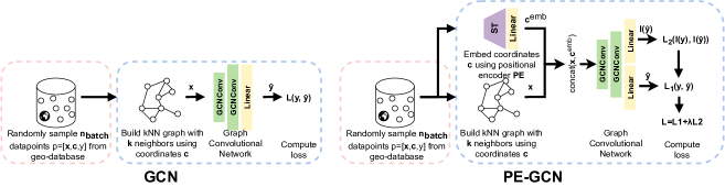
Figure 1: PE-GCN compared to the GCN baseline: PE-GCN contains a (1) positional encoder network, learning a spatial context embedding throughout training which is concatenated with node-level features and (2) an auxiliary learner, predicting the spatial autocorrelation of the outcome variable simultaneously to the main regression task.

3.1 Graph Neural Networks with Geographic Data

We now present PE-GNN, using Graph Convolutional Networks (GCNs) as example backbone. Let us first define a datapoint $p_{i}=\{y_{i},\mathbf{x_{i}},\mathbf{c_{i}}\}$, where $y_{i}$ is a continuous target variable (scalar), $\mathbf{x_{i}}$ is a vector of predictive features and $\mathbf{c_{i}}$ is a vector of point coordinates (latitude / longitude pairs). We use the great-circle distance $d_{ij}=haversin(\mathbf{c_{i}},\mathbf{c_{j}})$ between point coordinates to create a graph of all points in the set, using a $k$-nearest-neighbor approach to define each point’s neighborhood. The graph $G=(V,E)$ consists of a set of vertices (or nodes) $V=\{v_{1},\dots,v_{n}\}$ and a set of edges $E=\{e_{1},\dots,e_{m}\}$ as assigned by the adjacency matrix $\mathbf{A}$. Each vertex $i\in V$ has respective node features $\mathbf{x_{i}}$ and target variable $y_{i}$. While the adjacency matrix $\mathbf{A}$ usually comes as a binary matrix (with values of $1$ indicating adjacency and values of $0$ otherwise), one can account for different distances between nodes and use point distances $d_{ij}$ or kernel transformations thereof (Appleby et al., 2020) to weight $\mathbf{A}$. Given a degree matrix $\mathbf{D}$ and an identity matrix $\mathbf{I}$, the normalized adjacency matrix $\mathbf{\bar{A}}$ is defined as:

$$\mathbf{\bar{A}}=\mathbf{D}^{-1/2}(\mathbf{A}+\mathbf{I})\mathbf{D}^{-1/2}$$ (1)

As proposed by Kipf and Welling (2017), a GCN layer can now be defined as:

$$\mathbf{H}^{(l)}=\sigma(\mathbf{\bar{A}}\mathbf{H}^{(l-1)}\mathbf{W}^{(l)}),l=1,\dots,L$$ (2)

where $\sigma$ describes an activation function (e.g., ReLU) and $\mathbf{W}^{(l)}$ is a weight matrix parametrizing GCN layer $l$. The input for the first GCN layer $\mathbf{H^{(0)}}$ is given by the feature matrix $\mathbf{X}$ containing all node feature vectors $\mathbf{x_{1}},\dots,\mathbf{x_{n}}$. The assembled GCN predicts the output $\mathbf{\hat{Y}}=GCN(\mathbf{X},\Theta_{GCN})$ parametrized by $\Theta_{GCN}$.

3.2 Context-aware spatial coordinate embeddings

Traditionally, the only intuition for spatial context in GCNs stems from connections between nodes which allow for graph convolutions, akin to pixel convolutions with image data. This can restrict the capacity of the GCN to capture spatial patterns: While defining good neighborhood structures can be crucial for GCN performance, this often comes down to somewhat arbitrary choices like selecting the $k$ nearest neighbors of each node. Without prior knowledge on the underlying data, the process of setting the right neighborhood parameters may require extensive testing. Furthermore, a single value of $k$ might not be best for all nodes: different locations might be more or less dependent on their neighbors. Assuming that no underlying graph connecting point locations is known, one would typically construct a graph using the distance (Euclidean or other) between pairs of points. In many real world settings (e.g., points-of-interest along a road network) this assumption is unrealistic and may lead to poorly defined neighborhoods. Lastly, GCNs contain no intrinsic tool to transform point coordinates into a different (latent) space that might be more informative for representing the spatial structure, with respect to the particular problem the GCN is trying to solve.

As such, GCNs can struggle with tasks that explicitly require learning of complex spatial dependencies, as we confirm in our experiments. We propose a novel approach to overcome these difficulties, by devising a new positional encoder module, learning a flexible spatial context encoding for each geographic location. Given a batch of datapoints, we create the spatial coordinate matrix $\mathbf{C}$ from individual point coordinates $\mathbf{c_{1}},\dots,\mathbf{c_{n}}$ and define a positional encoder $PE(\mathbf{C},\sigma_{min},\sigma_{max},\Theta_{PE})=NN(ST(\mathbf{C},\sigma_{min}$, $\sigma_{max}),\Theta_{PE})$, consisting of a sinusoidal transform $ST(\sigma_{min}$, $\sigma_{max})$ and a fully-connected neural network $NN(\Theta_{PE})$, parametrized by $\Theta_{PE}$. Following the intuition of transformers (Vaswani et al., 2017) for geographic coordinates (Mai et al., 2020b), the sinusoidal transform is a concatenation of scale-sensitive sinusoidal functions at different frequencies, so that

$$ST(\mathbf{C},\sigma_{min},\sigma_{max})=$$ (3)

$$[ST_{0}(\mathbf{C},\sigma_{min},\sigma_{max});\dots;ST_{S-1}(\mathbf{C},\sigma_{min},\sigma_{max})]$$

with $S$ being the total number of grid scales and $\sigma_{min}$ and $\sigma_{max}$ setting the minimum and maximum grid scale (comparable to the lengthscale parameter of a kernel). The scale-specific encoder $ST_{s}(\mathbf{C},\sigma_{min},\sigma_{max})=[ST_{s,1}(\mathbf{C},\sigma_{min},\sigma_{max});ST_{s,2}(\mathbf{C},\sigma_{min},\sigma_{max})]$ processes the spatial dimensions $v$ (e.g., latitude and longitude) of $\mathbf{C}$ separately, so that

$$ST_{s,v}(\mathbf{C,\sigma_{min},\sigma_{max}})=$$ (4)

$$\left[\cos\left(\frac{\mathbf{C}^{[v]}}{\sigma_{min}g^{s/(S-1)}}\right);\sin\left(\frac{\mathbf{C}^{[v]}}{\sigma_{min}g^{s/(S-1)}}\right)\right]$$

$$\forall s\in\{0,\ldots,S-1\},\forall v\in\{1,2\},$$

where $g=\frac{\sigma_{max}}{\sigma_{min}}$. The output from $ST$ is then fed through the fully connected neural network $NN(\Theta_{PE})$ to transform it into the desired vector space shape, creating the coordinate embedding matrix $\mathbf{C}_{emb}=PE(\mathbf{C},\sigma_{min},\sigma_{max},\Theta_{PE})$.

3.3 Auxiliary learning of spatial autocorrelation

Geographic data often exhibit spatial autocorrelation: observations are related, in some shape or form, to their geographic neighbors. Spatial autocorrelation can be measured using the Moran’s I metric of local spatial autocorrelation (Anselin, 1995). Moran’s I captures localized homogeneity and outliers, functioning as a detector of spatial clustering and spatial change patterns. In the context of our problem, the Moran’s I measure of spatial autocorrelation for outcome variable $y_{i}$ is defined as:

$$\begin{split}I_{i}=(n-1)\frac{(y_{i}-\bar{y}_{i})}{\sum^{n}_{j=1}(y_{j}-\bar{y}_{j})^{2}}\sum^{n}_{j=1,j\neq i}a_{i,j}(y_{j}-\bar{y}_{j}),\end{split}$$ (5)

where $a_{i,j}\in\mathbf{A}$ denotes adjacency of observations $i$ and $j$.

As proposed by Klemmer and Neill (2021), predicting the Moran’s I metric of the output can be used as auxiliary task during training. Auxiliary task learning (Suddarth and Kergosien, 1990) is a special case of multi-task learning, where one learning algorithm tackles two or more tasks at once. In auxiliary task learning, we are only interested in the predictions of one task; however, adding additional, auxiliary tasks to the learner might improve performance on the primary problem: the auxiliary task can add context to the learning problem that can help solve the main problem. This approach is commonly used, for example in reinforcement learning (Flet-Berliac and Preux, 2019) or computer vision (Hou et al., 2019; Jaderberg et al., 2017).

Translated to our GCN setting, we seek to predict the outcome $\mathbf{Y}$ and its local Moran’s I metric $I(\mathbf{Y})$ using the same network, so that $[\hat{\mathbf{Y}},\hat{I(\mathbf{Y})}]=GCN(\mathbf{X})$. As Klemmer and Neill (2021) note, the local Moran’s I metric is scale-sensitive and, due to its restriction to local neighborhoods, can miss out on longer-distance spatial effects (Feng et al., 2019; Meng et al., 2014). But while Klemmer and Neill (2021) propose to compute the Moran’s I at different resolutions, the GCN setting allows for a different, novel approach to overcome this issue: Rather than constructing the graph of training points a priori, we opt for a procedure where in each training step, $n_{batch}$ points are sampled from the training data as batch $B$. A graph with corresponding adjacency matrix $\mathbf{A}_{B}$ is constructed for the batch and the Moran’s I metric of the outcome variable $I(\mathbf{Y}_{B})$ is computed. This approach brings a unique advantage: When training with (randomly shuffled) batches, points may have different neighbors in different training iterations. The Moran’s I for point $i$ can thus change throughout iterations, reflecting a differing set of more distant or closer neighbors. This also naturally helps to tackle Moran’s I scale sensitivity. Altogether, we refer to this altered Moran’s I as “shuffled Moran’s I”.

3.4 Positional Encoder Graph Neural Network (PE-GNN)

We now assemble the different modules of our method and introduce the Positional Encoder Graph Neural Network (PE-GNN). The whole modeling pipeline of PE-GNN compared to a naive GNN approach is pictured in Figure 1. Sticking to the GCN example, PE-GCN is constructed as follows: Assuming a batch $B$ of randomly sampled points $p_{1},\dots,p_{n_{batch}}\in B$, a spatial graph is constructed from point coordinates $\mathbf{c}_{1},\dots,\mathbf{c}_{n_{batch}}$ using $k$-nearest-neighborhood, resulting in adjacency matrix $\mathbf{A}_{B}$. The point coordinates are then subsequently fed through the positional encoder $PE(\Theta_{PE})$, consisting of the sinusoidal transform $ST$ and a single fully-connected layer with sigmoid activation, embedding the $2d$ coordinates in a custom latent space and returning vector embeddings $\mathbf{c}_{1}^{emb},\dots,\mathbf{c}_{n_{batch}}^{emb}=\mathbf{C}_{B}^{emb}$. The neural network allows for explicit learning of spatial context, reflected in the vector embedding. We then concatenate the positional encoder output with the node features, to create the input for the first GCN layer:

$$\mathbf{H}^{(0)}=concat(\mathbf{X}_{B},\mathbf{C}_{B}^{emb})$$ (6)

The subsequent layers follow according to Equation 2. Note here that this approach is distinctly different from Mai et al. (2020a), who learn a specific joint embedding between the geographic coordinates and potential other inputs (e.g., text data). Our approach allows for separate treatment of geographic coordinates and potential other predictors, allowing a higher degree of flexibility: PE-GCN can be deployed for any regression task, geo-referenced in the form of latitude longitude coordinates. Lastly, to integrate the Moran’s I auxiliary task, we compute the metric $I(\mathbf{Y}_{B})$ for our outcome variable $\mathbf{Y}_{B}$ at the beginning of each training step according to Equation 5, using spatial weights from $\mathbf{A}_{B}$. Prediction is then facilitated by creating two prediction heads, here linear layers, while the graph operation layers (e.g., GCN layers) are shared between tasks. Finally, we obtain predicted values $\hat{\mathbf{Y}}_{B}$ and $\hat{I(\mathbf{Y}_{B})}$. The loss of PE-GCN can be computed with any regression criterion, for example mean squared error (MSE):

$$\mathcal{L}=MSE(\hat{\mathbf{Y}}_{B},\mathbf{Y}_{B})+\lambda MSE(I(\hat{\mathbf{Y}}_{B}),I(\mathbf{Y}_{B}))$$ (7)

where $\lambda$ denotes the auxiliary task weight. The final model is denoted as $M_{\Theta_{PE},\Theta_{GCN}}$. Algorithm 1 describes a training cycle.

Algorithm 1 PE-GNN Training

1:$M$, $\lambda$, $k$, $tsteps$,$n_{batch}$ hyper-parameter

2:Initialize model $M$ with random weights and hyper-parameter

3:Set optimizer with hyper-parameter

4:for number of training steps ($tsteps$) do

5:     Sample minibatch $B$ of $n_{batch}$ points with features $\mathbf{X}_{B}$, coordinates $\mathbf{C}_{B}$ and outcome $\mathbf{Y}_{B}$.

6:     Construct a spatial graph with adjacency matrix $\mathbf{A}_{B}$ from coordinates $\mathbf{C}_{B}$ using $k$-nearest neighbors

7:     Using spatial adjacency $\mathbf{A}_{B}$, compute Moran’s I of output as $I(\mathbf{Y}_{B})$

8:     Predict outcome

9:$[\hat{\mathbf{Y}}_{B},I(\hat{\mathbf{Y}}_{B})]=M_{\Theta_{PE},\Theta_{GCN}}(\mathbf{X}_{B},\mathbf{C}_{B},\mathbf{A}_{B})$

10:     Compute loss

11:$\mathcal{L}(\mathbf{Y}_{B},I(\mathbf{Y}_{B}),\hat{\mathbf{Y}}_{B},I(\hat{\mathbf{Y}}_{B}),\lambda)$

12:     Update the parameters $\Theta_{GCN},\Theta_{PE}$ of model $M$ using stochastic gradient descent

13:return $M$

We begin training by initializing our model $M$, for example a PE-GCN, with random weights and potential hyper-parameters (e.g., PE embedding dimension) and defining our optimizer. We then start the training cycle: At each training step, we first sample a minibatch $B$ of points from our training data. These points come as features $\mathbf{X}_{B}$, point coordinates $\mathbf{C}_{B}$ and outcome variables $\mathbf{Y}_{B}$. We construct a graph from spatial coordinates $\mathbf{C}_{B}$ using $k$-nearest-neighborhood, obtaining an adjacency matrix $\mathbf{A}_{B}$. Next we use $\mathbf{A}_{B}$ as spatial weight matrix to compute local Moran’s I values $I(\mathbf{Y}_{B})$ from $\mathbf{Y}_{B}$. As minibatches are randomly sampled, this creates a “shuffled” version of the metric. We then run inputs $\mathbf{X}_{B},\mathbf{C}_{B},\mathbf{A}_{B}$ through the two-headed model $M_{\Theta_{PE},\Theta_{GCN}}$ obtaining predictions $\hat{\mathbf{Y}}_{B},I(\hat{\mathbf{Y}}_{B})$. We then compute the loss $\mathcal{L}(\mathbf{Y}_{B},I(\mathbf{Y}_{B}),\hat{\mathbf{Y}}_{B},I(\hat{\mathbf{Y}}_{B}),\lambda)$, weighing the Moran’s I auxiliary task according to weight parameter $\lambda$. Lastly, we use the loss $\mathcal{L}$ to update our model parameters $\Theta_{GCN},\Theta_{PE}$ according to stochastic gradient descent. Training is conducted for $tsteps$ after which the final model $M$ is returned.

PE-GNN, with any GNN backbone, helps to tackle many of the particular challenges of geographic data: While our approach still includes the somewhat arbitrary choice of $k$-nearest neighbors to define the spatial graph, the proposed positional encoder network is not bound by this restriction, as it does not operate on the graph. This enables a separate learning of context-aware embeddings for each coordinate, accounting for neighbors at any potential distance within the batch. While the spatial graph used still relies on pre-defined distance measure, the positional encoder embeds latitude and longitude values in a high-dimensional latent space. These high-dimensional coordinates are able to reflect spatial complexities much more flexibly and, added as node features, can communicate these throughout the learning process. Batched PE-GNN training is not conducted on a single graph, but a new graph consisting of randomly sampled training points at each iteration. As such, at different iterations, focus is put on the relationships between different clusters of points. This helps our method to generalize better, rather than just memorizing neighborhood structures. Lastly, the differing training batches also help us to compute a “shuffled” version of the Moran’s I metric, capturing autocorrelation at the same location for different (closer or more distant), random neighborhoods.

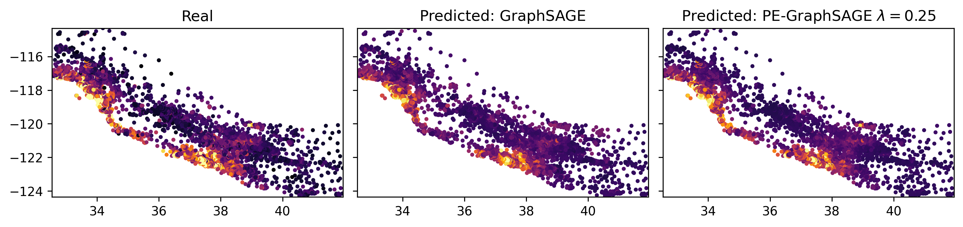
(a) Real values and predictions using GraphSAGE and PE-GraphSAGE.

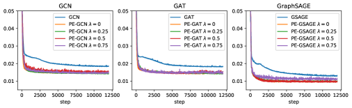
(b) Test error curves of GCN, GAT and GraphSAGE based models, measured by the MSE metric.

Figure 2: Visualizing predictive performance on the California Housing dataset.

4 Experiments

Model	Cali. Housing		Election		Air Temp.		3d Road
	MSE	MAE	MSE	MAE	MSE	MAE	MSE	MAE
GCN Kipf and Welling (2017)	0.0558	0.1874	0.0034	0.0249	0.0225	0.1175	0.0169	0.1029
PE-GCN $\lambda=0$	0.0161	0.0868	0.0032	0.0241	0.0040	0.0432	0.0031	0.0396
PE-GCN $\lambda=0.25$	0.0155	0.0882	0.0032	0.0236	0.0037	0.0417	0.0032	0.0416
PE-GCN $\lambda=0.5$	0.0156	0.0885	0.0031	0.0241	0.0036	0.0401	0.0033	0.0421
PE-GCN $\lambda=0.75$	0.0160	0.0907	0.0031	0.0240	0.0040	0.0429	0.0033	0.0424
GAT Veličković et al. (2018)	0.0558	0.1877	0.0034	0.0249	0.0226	0.1165	0.0178	0.0998
PE-GAT $\lambda=0$	0.0159	0.0918	0.0032	0.0234	0.0039	0.0429	0.0060	0.0537
PE-GAT $\lambda=0.25$	0.0161	0.0867	0.0032	0.0235	0.0040	0.0417	0.0058	0.0530
PE-GAT $\lambda=0.5$	0.0162	0.0897	0.0032	0.0238	0.0045	0.0465	0.0061	0.0548
PE-GAT $\lambda=0.75$	0.0162	0.0873	0.0032	0.0237	0.0041	0.0429	0.0062	0.0562
GraphSAGE Hamilton et al. (2017)	0.0558	0.1874	0.0034	0.0249	0.0274	0.1326	0.0180	0.0998
PE-GraphSAGE $\lambda=0$	0.0157	0.0896	0.0032	0.0237	0.0039	0.0428	0.0060	0.0534
PE-GraphSAGE $\lambda=0.25$	0.0097	0.0664	0.0032	0.0242	0.0040	0.0418	0.0059	0.0534
PE-GraphSAGE $\lambda=0.5$	0.0100	0.0682	0.0033	0.0239	0.0043	0.0461	0.0060	0.0536
PE-GraphSAGE $\lambda=0.75$	0.0100	0.0661	0.0032	0.0241	0.0036	0.0399	0.0058	0.0541
KCN Appleby et al. (2020)	0.0292	0.1405	0.0367	0.1875	0.0143	0.0927	0.0081	0.0758
PE-KCN $\lambda=0$	0.0288	0.1274	0.0598	0.2387	0.0648	0.2385	0.0025	0.0310
PE-KCN $\lambda=0.25$	0.0324	0.1380	0.0172	0.1246	0.0059	0.0593	0.0037	0.0474
PE-KCN $\lambda=0.5$	0.0237	0.1117	0.0072	0.0714	0.0077	0.0664	0.0077	0.0642
PE-KCN $\lambda=0.75$	0.0260	0.1194	0.0063	0.0681	0.0122	0.0852	0.0110	0.0755
Approximate GP	0.0353	0.1382	0.0031	0.0348	0.0481	0.0498	0.0080	0.0657
Exact GP	0.0132	0.0736	0.0022	0.0253	0.0084	0.0458	-	-

Table 1: Spatial Interpolation: Test MSE and MAE scores from four different datasets, using four different GNN backbones with and without our proposed architecture.

Model	Cali. Housing		Election		Air Temp.
	MSE	MAE	MSE	MAE	MSE	MAE
GCN	0.0185	0.1006	0.0025	0.0211	0.0225	0.1175
PE-GCN $\lambda=0$	0.0143	0.0814	0.0026	0.0213	0.0040	0.0432
PE-GCN $\lambda=0.25$	0.0143	0.0816	0.0026	0.0213	0.0037	0.0417
PE-GCN $\lambda=0.5$	0.0143	0.0828	0.0027	0.0217	0.0036	0.0401
PE-GCN $\lambda=0.75$	0.0147	0.0815	0.0027	0.0219	0.0040	0.0429
GAT	0.0183	0.0969	0.0024	0.0211	0.0226	0.1165
PE-GAT $\lambda=0$	0.0144	0.0836	0.0028	0.0218	0.0039	0.0429
PE-GAT $\lambda=0.25$	0.0141	0.0817	0.0028	0.0219	0.0040	0.0417
PE-GAT $\lambda=0.5$	0.0155	0.0851	0.0030	0.0225	0.0045	0.0465
PE-GAT $\lambda=0.75$	0.0145	0.0824	0.0029	0.0223	0.0041	0.0429
G.SAGE	0.0131	0.0798	0.0007	0.0127	0.0219	0.1153
PE-G.SAGE $\lambda=0$	0.0099	0.0667	0.0011	0.0154	0.0037	0.0422
PE-G.SAGE $\lambda=0.25$	0.0098	0.0648	0.0010	0.0152	0.0029	0.0381
PE-G.SAGE $\lambda=0.5$	0.0098	0.0679	0.0012	0.0157	0.0037	0.0445
PE-G.SAGE $\lambda=0.75$	0.0114	0.0766	0.0012	0.0152	0.0038	0.0459
KCN	0.0292	0.1405	0.0367	0.1875	0.0143	0.0927
PE-KCN $\lambda=0$	0.0288	0.1274	0.0598	0.2387	0.0648	0.2385
PE-KCN $\lambda=0.25$	0.0324	0.1380	0.0172	0.1246	0.0059	0.0593
PE-KCN $\lambda=0.5$	0.0237	0.1117	0.0072	0.0714	0.0077	0.0664
PE-KCN $\lambda=0.75$	0.0260	0.1194	0.0063	0.0681	0.0122	0.0852
Approximate GP	0.0195	0.1008	0.0050	0.0371	0.0481	0.0498
Exact GP	0.0036	0.0375	0.0006	0.0139	0.0084	0.0458

Table 2: Spatial Regression: Test MSE and MAE scores from three different datasets, using four different GNN backbones with and without our proposed architecture.

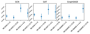
(a) California Housing.

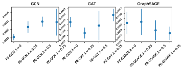
(b) 3d Road.

Figure 3: MSE bar plots of mean performance and $2\sigma$ confidence intervals obtained from 10 different training checkpoints.

4.1 Data

We evaluate PE-GNN and baseline competitors on four real-world geographic datasets of different spatial resolutions (regional, continental and global):
California Housing: This dataset contains the prices of over $20,000$ California houses from the 1990 U.S. census (Kelley Pace and Barry, 2003). The regression task at hand is to predict house prices $y$ using features $\mathbf{x}$ (e.g., house age, number of bedrooms) and location $\mathbf{c}$. California housing is a standard dataset for assessment of spatial autocorrelation.
Election:This dataset contains the election results of over $3,000$ counties in the United States (Jia and Benson, 2020). The regression task here is to predict election outcomes $y$ using socio-demographic and economic features (e.g., median income, education) $\mathbf{x}$ and county locations $\mathbf{c}$.
Air temperature:The air temperature dataset (Hooker et al., 2018) contains the coordinates of  $3,000$ weather stations around the globe. For this regression task we seek to predict mean temperatures $y$ from a single node feature $x$, mean precipitation, and location $c$.
3d Road:The 3d road dataset (Kaul et al., 2013) provides $3$-dimensional spatial co-ordinates (latitude, longitude, and altitude) of the road network in Jutland, Denmark. The dataset comprises over $430,000$ points and can be used for interpolating altitude $y$ using only latitude and longitude coordinates $\mathbf{c}$ (no node features $x$).

4.2 Experimental setup

We compare PE-GNN with four different graph neural network backbones: The original GCN formulation (Kipf and Welling, 2017), graph attention mechanisms (GAT) (Veličković et al., 2018) and GraphSAGE (Hamilton et al., 2017). We also use Kriging Convolutional Networks (KCN) (Appleby et al., 2020), which differs from GCN primarily in two ways: it transforms the distance-weighted adjacency matrix $\mathbf{A}$ using a Gaussian kernel and adds the outcome variable and features of neighboring points to the features of each node. Test set points can only access neighbors from the training set to extract these features. We compare the naive version of all these approaches to the same four backbone architectures augmented with our PE-GNN modules. Beyond GNN-based approaches, we also compare PE-GNN to the most popular method for modeling continuous spatial data: Gaussian processes. For all approaches, we compare a range of different training settings and hyperparameters, as discussed below.

To allow for a fair comparison between the different approaches, we equip all models with the same architecture, consisting of two GCN / GAT / GraphSAGE layers with ReLU activation and dropout, followed by linear layer regression heads. The KCN model also uses GCN layers, following the author specifications. We found that adding additional layers to the GNNs did not increase their capacity for processing raw latitude / longitude coordinates. We test four different auxiliary task weights $\lambda=\{0,0.25.0.5,0.75\}$, where $\lambda=0$ implies no auxiliary task. Spatial graphs are constructed assuming $k=5$ nearest neighbors, following rigorous testing. This also confirms findings from previous work (Appleby et al., 2020; Jia and Benson, 2020). We include a sensitivity analysis of the $k$ parameter and different batch sizes in our results section. Training for the GNN models is conducted using PyTorch (Paszke et al., 2019) and PyTorch Geometric (Fey and Lenssen, 2019). We use the Adam algorithm to optimize our models (Kingma and Ba, 2015) and the mean squared error (MSE) loss. Gaussian process models (exact and approximate) are trained using GPyTorch (Gardner et al., 2018). Due to the size of the dataset, we only provide an approximate GP result for 3d Road. All training is conducted on single CPU. On the Cali. Housing dataset ($n>20,000$) training times for one step (no batched training) are as follows: PE-GCN = $0.23s$ (with aux. task $0.24s$), PE-GAT = $0.38s$, PE-GraphSAGE = $0.33s$, PE-KCN = $0.41$, exact GP = $0.77s$. Results are averaged over $100$ training steps. The code for PE-GNN and our experiments can be accessed here: https://github.com/konstantinklemmer/pe-gnn.

4.3 Results

4.3.1 Predictive performance

We test our methods on two tasks: Spatial Interpolation, predicting outcomes from spatial coordinates alone, and Spatial Regression, where other node features are available in addition to the latitude / longitude coordinates. The results of our experiments are shown in Table 1 and 2. For all models, we provide mean squared error (MSE) and mean absolute error (MAE) metrics on held-out test data. For the spatial interpolation task, we observe that the PE-GNN approaches consistently and vastly improve performance for all four backbone architectures across the California Housing, Air Temperature and 3d Road datasets and, by a small margin, for the Election dataset. For the spatial regression task, we observe that the PE-GNN approaches consistently and substantially improve performance for all four backbone architectures on the California Housing and Air Temperature datasets. Performance remains unchanged or decreases by very small margins in the Election dataset, except for the KCN backbone which benefits tremendously from the PE-GNN approach, particularly with auxiliary tasks.

Generally, PE-GNN substantially improves over baselines in regression and interpolation settings. Most of the improvement can be attributed to the positional encoder, however the auxiliary task learning also has substantial beneficial effects in some settings, especially for the KCN models. The best setting for the task weight hyperparameter $\lambda$ seems to heavily depend on the data, which confirms findings by Klemmer and Neill (2021). To our knowledge, PE-GNN is the first GNN-based learning approach that can compete with Gaussian Processes on simple spatial interpolation baselines, though especially exact GPs still sometimes have the edge. PE-GNN is substantially more scalable than exact GPs, which rely on expensive pair-wise distance calculations across the full training dataset. Due to this problem, we do not run an exact GP baseline for the high-dimensional 3d Road dataset. For KCN models, we observe a proneness to overfitting. As the authors of KCN mention, this effect diminishes in large enough data domains (Appleby et al., 2020). For example, KCNs are the best performing method on the 3d Road dataset–by far our largest experimental dataset. Here, we also observe that in cases when KCN learns well, PE-KCN can still improve its performance. The KCN experiments also highlight the strongest effects of the Moran’s I auxiliary tasks: In cases when KCN overfits (Election, Cali. Housing datasets), PE-KCN without auxiliary task ($\lambda=0$) is not sufficient to overcome the problem. However, adding the auxiliary task can mitigate most of the overfitting issue. This directly confirms a theory of Klemmer and Neill (2021) on the beneficial effects of auxiliary learning of spatial autocorrelation. Regarding the question of spatial scale, we find no systemic variation in PE-GNN performance between applications with regional (California Housing, 3d Road), continental (Election) and global (Air Temperature) spatial coverage. PE-GNN performance depends on the difficulty of the task at hand and the complexity of present spatial dependencies.

We also assess the robustness of PE-GNN training cycles. Figure 3 highlights the confidence intervals of PE-GNN models with GCN, GAT and GraphSAGE backbones trained on the California Housing and 3d Road datasets, obtained from 10 different training cycles. We can see that training runs exhibit only little variability. These findings thus confirm that PE-GNN can consistently outperform naive GNN baselines.

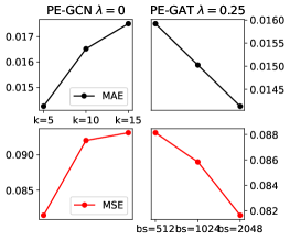
Figure 4: Predictive performance of PE-GCN and PE-GAT models on the California Housing dataset, using different values of $k$ for constructing nearest-neighbor graphs and different batch sizes (bs).

4.3.2 Sensitivity analyses

Figure 4 highlights some results from our sensitivity analyses with the $k$ and $n_{batch}$ (batch size) parameters. After rigorous testing, we opt for $k=5$-NN approach to create the spatial graph and compute the shuffled Moran’s I across all models. We chose $n_{batch}=2048$ for Cali. Housing and 3d Road datasets and $n_{batch}=1024$ for the Election and Air Temperature datasets. Note that while our experiments focus on batched training to highlight the applicability of PE-GNN to high-dimensional geospatial datasets, we also tested our approach with non-batched training on the smaller datasets (Election, Air Temperature, California Housing). We found only marginal performance differences between these settings.

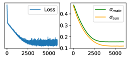
Figure 5: Automatic learning of loss weights via task uncertainty on the Air Temp. dataset with PE-GCN. The left graphic shows the training loss (MSE), while the right graphic shows the main and auxiliary task weight parameters $\sigma_{main}$ and $\sigma_{aux}$. The training steps are given on the x-axis.

4.3.3 Learning auxiliary loss weights using task uncertainty

Lastly, following work by Cipolla et al. (2018) and Klemmer and Neill (2021), we provide an intuition for automatically selecting the Moran’s I auxiliary task weights using task uncertainty. This eliminates the need to manually tune and select the $\lambda$ parameter. The approach first proposed by Cipolla et al. (2018) formalizes the idea by first defining a probabilistic multi-task regression problem with a main and auxiliary task as:

$$p(\hat{\mathbf{Y}}_{main},\hat{\mathbf{Y}}_{aux}|f(\mathbf{X}))=p(\hat{\mathbf{Y}}_{main}|f(\mathbf{X}))p(\hat{\mathbf{Y}}_{aux}|f(\mathbf{X}))$$ (8)

with $\hat{\mathbf{Y}}_{main},\hat{\mathbf{Y}}_{aux}$ giving the main and auxiliary task predictions. Following maximum likelihood estimation, the regression objective function is given as $\min\mathcal{L}(\sigma_{main},\sigma_{aux})$:

$$=-\log p(\hat{\mathbf{Y}}_{main},\hat{\mathbf{Y}}_{aux}|f(\mathbf{X}))$$ (9)

$$=\frac{1}{2\sigma_{main}^{2}}\mathcal{L}_{main}+\frac{1}{2\sigma_{aux}^{2}}\mathcal{L}_{aux}+$$

$$(\log\sigma_{main}+\log\sigma_{aux}),$$

with $\sigma_{main}$ and $\sigma_{aux}$ defining the model noise parameters. By minimizing this objective, we learn the relative weight or contribution of main and auxiliary task to the combined loss. The last term of the loss prevents it from moving towards infinity and acts as a regularizer. While this approach performs equally compared to a well selected $\lambda$ parameter, it eliminates the need to manually tune and select $\lambda$. Figure 5 highlights the learning of $\sigma_{main}$ and $\sigma_{aux}$ loss weights using PE-GCN and the Air Temperature dataset.

5 Conclusion

With PE-GNN, we introduce a flexible, modular GNN-based learning framework for geographic data. PE-GNN leverages recent findings in embedding spatial context into neural networks to improve predictive models. Our empirical findings confirm a strong performance. This study highlights how domain expertise can help improve machine learning models for applications with distinct characteristics. We hope to build on the foundations of PE-GNN to develop further methods for geospatial machine learning.

References

- (1)
- Anselin (1995) Luc Anselin. 1995. Local Indicators of Spatial Association—LISA. Geographical Analysis 27, 2 (sep 1995), 93–115. https://doi.org/10.1111/j.1538-4632.1995.tb00338.x arXiv:1011.1669
- Anselin et al. (2001) Luc Anselin et al. 2001. Spatial econometrics. A companion to theoretical econometrics 310330 (2001).
- Appleby et al. (2020) Gabriel Appleby, Linfeng Liu, and Li Ping Liu. 2020. Kriging convolutional networks. In AAAI 2020 - 34th AAAI Conference on Artificial Intelligence, Vol. 34. AAAI press, 3187–3194. https://doi.org/10.1609/aaai.v34i04.5716
- Chen et al. (2019) Cen Chen, Kenli Li, Sin G. Teo, Xiaofeng Zou, Kang Wang, Jie Wang, and Zeng Zeng. 2019. Gated residual recurrent graph neural networks for traffic prediction. In 33rd AAAI Conference on Artificial Intelligence, AAAI 2019, 31st Innovative Applications of Artificial Intelligence Conference, IAAI 2019 and the 9th AAAI Symposium on Educational Advances in Artificial Intelligence, EAAI 2019, Vol. 33. AAAI Press, 485–492. https://doi.org/10.1609/aaai.v33i01.3301485
- Cipolla et al. (2018) Roberto Cipolla, Yarin Gal, and Alex Kendall. 2018. Multi-task Learning Using Uncertainty to Weigh Losses for Scene Geometry and Semantics. In Proceedings of the IEEE Computer Society Conference on Computer Vision and Pattern Recognition. https://doi.org/10.1109/CVPR.2018.00781 arXiv:1705.07115
- Datta et al. (2016) Abhirup Datta, Sudipto Banerjee, Andrew O. Finley, and Alan E. Gelfand. 2016. Hierarchical Nearest-Neighbor Gaussian Process Models for Large Geostatistical Datasets. J. Amer. Statist. Assoc. 111, 514 (apr 2016), 800–812. https://doi.org/10.1080/01621459.2015.1044091
- Feng et al. (2019) Yongjiu Feng, Lijuan Chen, and Xinjun Chen. 2019. The impact of spatial scale on local Moran’s I clustering of annual fishing effort for Dosidicus gigas offshore Peru. Journal of Oceanology and Limnology 37, 1 (jan 2019), 330–343. https://doi.org/10.1007/s00343-019-7316-9
- Fey and Lenssen (2019) Matthias Fey and Jan Eric Lenssen. 2019. Fast Graph Representation Learning with PyTorch Geometric. (mar 2019). arXiv:1903.02428 http://arxiv.org/abs/1903.02428
- Flet-Berliac and Preux (2019) Yannis Flet-Berliac and Philippe Preux. 2019. MERL: Multi-Head Reinforcement Learning. In NeurIPS 2019 - Deep Reinforcement Learning Workshop. arXiv:1909.11939 http://arxiv.org/abs/1909.11939
- Fu et al. (2019) Yanjie Fu, Pengyang Wang, Jiadi Du, Le Wu, and Xiaolin Li. 2019. Efficient region embedding with multi-view spatial networks: A perspective of locality-constrained spatial autocorrelations. In 33rd AAAI Conference on Artificial Intelligence, AAAI 2019, 31st Innovative Applications of Artificial Intelligence Conference, IAAI 2019 and the 9th AAAI Symposium on Educational Advances in Artificial Intelligence, EAAI 2019, Vol. 33. AAAI Press, 906–913. https://doi.org/10.1609/aaai.v33i01.3301906
- Gardner et al. (2018) Jacob R. Gardner, Geoff Pleiss, David Bindel, Kilian Q. Weinberger, and Andrew Gordon Wilson. 2018. GPyTorch: Blackbox Matrix-Matrix Gaussian Process Inference with GPU Acceleration. In Advances in Neural Information Processing Systems (NeurIPS). arXiv:1809.11165 http://arxiv.org/abs/1809.11165
- Hamilton et al. (2017) William L. Hamilton, Rex Ying, and Jure Leskovec. 2017. Inductive representation learning on large graphs. In Advances in Neural Information Processing Systems, Vol. 2017-Decem. Neural information processing systems foundation, 1025–1035. arXiv:1706.02216 http://arxiv.org/abs/1706.02216
- Hooker et al. (2018) Josh Hooker, Gregory Duveiller, and Alessandro Cescatti. 2018. Data descriptor: A global dataset of air temperature derived from satellite remote sensing and weather stations. Scientific Data 5, 1 (nov 2018), 1–11. https://doi.org/10.1038/sdata.2018.246
- Hou et al. (2019) Yuenan Hou, Zheng Ma, Chunxiao Liu, and Chen Change Loy. 2019. Learning to Steer by Mimicking Features from Heterogeneous Auxiliary Networks. Proceedings of the AAAI Conference on Artificial Intelligence 33, 01 (jul 2019), 8433–8440. https://doi.org/10.1609/aaai.v33i01.33018433 arXiv:1811.02759
- Jaderberg et al. (2017) Max Jaderberg, Volodymyr Mnih, Wojciech Marian Czarnecki, Tom Schaul, Joel Z Leibo, David Silver, and Koray Kavukcuoglu. 2017. Reinforcement learning with unsupervised auxiliary tasks. In International Conference on Learning Representations (ICLR). arXiv:1611.05397 https://youtu.be/Uz-zGYrYEjA
- Jia and Benson (2020) Junteng Jia and Austion R. Benson. 2020. Residual Correlation in Graph Neural Network Regression. In Proceedings of the ACM SIGKDD International Conference on Knowledge Discovery and Data Mining. Association for Computing Machinery, New York, NY, USA, 588–598. https://doi.org/10.1145/3394486.3403101 arXiv:2002.08274
- Kaul et al. (2013) Manohar Kaul, Bin Yang, and Christian S. Jensen. 2013. Building accurate 3D spatial networks to enable next generation intelligent transportation systems. In Proceedings - IEEE International Conference on Mobile Data Management. https://doi.org/10.1109/MDM.2013.24
- Kelley Pace and Barry (2003) R. Kelley Pace and Ronald Barry. 2003. Sparse spatial autoregressions. Statistics & Probability Letters 33, 3 (may 2003), 291–297. https://doi.org/10.1016/s0167-7152(96)00140-x
- Kingma and Ba (2015) Diederik P Kingma and Jimmy Lei Ba. 2015. Adam: A method for stochastic optimization. In 3rd International Conference on Learning Representations, ICLR 2015 - Conference Track Proceedings. arXiv:1412.6980
- Kipf and Welling (2017) Thomas N. Kipf and Max Welling. 2017. Semi-supervised classification with graph convolutional networks. In 5th International Conference on Learning Representations, ICLR 2017 - Conference Track Proceedings. International Conference on Learning Representations, ICLR. arXiv:1609.02907 http://arxiv.org/abs/1609.02907
- Klemmer et al. (2019) Konstantin Klemmer, Adriano Koshiyama, and Sebastian Flennerhag. 2019. Augmenting correlation structures in spatial data using deep generative models. arXiv:1905.09796 (2019). arXiv:1905.09796 http://arxiv.org/abs/1905.09796
- Klemmer and Neill (2021) Konstantin Klemmer and Daniel B. Neill. 2021. Auxiliary-task learning for geographic data with autoregressive embeddings. In SIGSPATIAL: Proceedings of the ACM International Symposium on Advances in Geographic Information Systems.
- Klemmer et al. (2022) Konstantin Klemmer, Tianlin Xu, Beatrice Acciaio, and Daniel B. Neill. 2022. SPATE-GAN: Improved Generative Modeling of Dynamic Spatio-Temporal Patterns with an Autoregressive Embedding Loss. In AAAI 2022 - 36th AAAI Conference on Artificial Intelligence. arXiv:2109.15044v1
- Mai et al. (2020a) Gengchen Mai, Krzysztof Janowicz, Ling Cai, Rui Zhu, Blake Regalia, Bo Yan, Meilin Shi, and Ni Lao. 2020a. SE-KGE: A location-aware Knowledge Graph Embedding model for Geographic Question Answering and Spatial Semantic Lifting. Transactions in GIS 24 (6 2020), 623–655. Issue 3. https://doi.org/10.1111/TGIS.12629
- Mai et al. (2020b) Gengchen Mai, Krzysztof Janowicz, Bo Yan, Rui Zhu, Ling Cai, and Ni Lao. 2020b. Multi-Scale Representation Learning for Spatial Feature Distributions using Grid Cells. In International Conference on Learning Representations (ICLR). arXiv:2003.00824 http://arxiv.org/abs/2003.00824
- Meng et al. (2014) Yan Meng, Chao Lin, Weihong Cui, and Jian Yao. 2014. Scale selection based on Moran’s i for segmentation of high resolution remotely sensed images. In International Geoscience and Remote Sensing Symposium (IGARSS). Institute of Electrical and Electronics Engineers Inc., 4895–4898. https://doi.org/10.1109/IGARSS.2014.6947592
- Ord and Getis (2012) J. Keith Ord and Arthur Getis. 2012. Local spatial heteroscedasticity (LOSH). Annals of Regional Science 48, 2 (apr 2012), 529–539. https://doi.org/10.1007/s00168-011-0492-y
- Paszke et al. (2019) Adam Paszke, Sam Gross, Francisco Massa, Adam Lerer, James Bradbury, Gregory Chanan, Trevor Killeen, Zeming Lin, Natalia Gimelshein, Luca Antiga, Alban Desmaison, Andreas Köpf, Edward Yang, Zach DeVito, Martin Raison, Alykhan Tejani, Sasank Chilamkurthy, Benoit Steiner, Lu Fang, Junjie Bai, and Soumith Chintala. 2019. PyTorch: An imperative style, high-performance deep learning library. In Advances in Neural Information Processing Systems, Vol. 32. arXiv:1912.01703
- Suddarth and Kergosien (1990) S. C. Suddarth and Y. L. Kergosien. 1990. Rule-injection hints as a means of improving network performance and learning time. In Lecture Notes in Computer Science (including subseries Lecture Notes in Artificial Intelligence and Lecture Notes in Bioinformatics), Vol. 412 LNCS. Springer Verlag, 120–129. https://doi.org/10.1007/3-540-52255-7_33
- Vaswani et al. (2017) Ashish Vaswani, Noam Shazeer, Niki Parmar, Jakob Uszkoreit, Llion Jones, Aidan N. Gomez, Łukasz Kaiser, and Illia Polosukhin. 2017. Attention is all you need. In Advances in Neural Information Processing Systems, Vol. 2017-Decem. 5999–6009. arXiv:1706.03762 https://research.google/pubs/pub46201/
- Veličković et al. (2018) Petar Veličković, Arantxa Casanova, Pietro Liò, Guillem Cucurull, Adriana Romero, and Yoshua Bengio. 2018. Graph attention networks. In 6th International Conference on Learning Representations, ICLR 2018 - Conference Track Proceedings. International Conference on Learning Representations, ICLR. arXiv:1710.10903 https://arxiv.org/abs/1710.10903v3
- Wang et al. (2017) Fengjiao Wang, Chun Ta Lu, Yongzhi Qu, and Philip S. Yu. 2017. Collective geographical embedding for geolocating social network users. In Lecture Notes in Computer Science (including subseries Lecture Notes in Artificial Intelligence and Lecture Notes in Bioinformatics). Vol. 10234 LNAI. Springer Verlag, 599–611. https://doi.org/10.1007/978-3-319-57454-7_47
- Westerholt et al. (2018) Rene Westerholt, Bernd Resch, Franz Benjamin Mocnik, and Dirk Hoffmeister. 2018. A statistical test on the local effects of spatially structured variance. International Journal of Geographical Information Science 32, 3 (mar 2018), 571–600. https://doi.org/10.1080/13658816.2017.1402914
- Yin et al. (2019) Yifang Yin, Zhenguang Liu, Ying Zhang, Sheng Wang, Rajiv Ratn Shah, and Roger Zimmermann. 2019. GPS2Vec: Towards generating worldwide GPS embeddings. In SIGSPATIAL: Proceedings of the ACM International Symposium on Advances in Geographic Information Systems. Association for Computing Machinery, New York, NY, USA, 416–419. https://doi.org/10.1145/3347146.3359067
- Zhu et al. (2020) Di Zhu, Fan Zhang, Shengyin Wang, Yaoli Wang, Ximeng Cheng, Zhou Huang, and Yu Liu. 2020. Understanding Place Characteristics in Geographic Contexts through Graph Convolutional Neural Networks. Annals of the American Association of Geographers 110, 2 (mar 2020), 408–420. https://doi.org/10.1080/24694452.2019.1694403