Graph Neural Networks with Feature and Structure Aware Random Walk

Abstract.

Graph Neural Networks (GNNs) have received increasing attention for representation learning in various machine learning tasks. However, most existing GNNs applying neighborhood aggregation usually perform poorly on the graph with heterophily where adjacent nodes belong to different classes. In this paper, we show that in typical heterphilous graphs, the edges may be directed, and whether to treat the edges as is or simply make them undirected greatly affects the performance of the GNN models. Furthermore, due to the limitation of heterophily, it is highly beneficial for the nodes to aggregate messages from similar nodes beyond local neighborhood.These motivate us to develop a model that adaptively learns the directionality of the graph, and exploits the underlying long-distance correlations between nodes. We first generalize the graph Laplacian to digraph based on the proposed Feature-Aware PageRank algorithm, which simultaneously considers the graph directionality and long-distance feature similarity between nodes. Then digraph Laplacian defines a graph propagation matrix that leads to a model called DiglacianGCN. Based on this, we further leverage the node proximity measured by commute times between nodes, in order to preserve the nodes’ long-distance correlation on the topology level. Extensive experiments on ten datasets with different levels of homophily demonstrate the effectiveness of our method over existing solutions in the task of node classification.

1. Introduction

GNNs have demonstrated remarkable performance in a wide spectrum of graph-based tasks, such as node classification (Kipf and Welling, 2017; Hamilton et al., 2017), link prediction (Zhang and Chen, 2018) and community detection (Chen et al., 2019). Among the plentiful models that have been proposed, message passing neural networks (MPNNs) (Gilmer et al., 2017) have been by far the most widely adopted. The main idea of MPNN-based GNNs is that each node aggregates messages from its neighbors and utilizes these messages to update its representation.

Despite its success, such a recursively neighbor aggregating schema is susceptible to the quality of the graph. Specifically, MPNN-based GNNs rely on the assumption of homophily (Zhu et al., 2020b) as a strong inductive bias, i.e., adjacent nodes tend to belong to the same class. However, homophily is not a universal principle, and there exists networks exhibiting heterophily, where a significant portion of edges connect nodes with different classes. Simply applying typical MPNN-based GNNs to a heterophilous graph would result in a huge drop in effectiveness. For example, in social networks, the unique attributes of celebrities would be diluted if aggregated with the attributes of their followers. Hence, how to design a GNN architecture that works both for homophilous and heterophilous graphs has been a challenging topic recently.

Prior work and limitations. A direct way to overcome the limitation of heterophily is to stack multiple GNN layers (Abu-El-Haija et al., 2019; Ming Chen et al., 2020; Xu et al., 2018). However, stacking layers may bring increasing parameters, causing the risks of overfitting, vanishing gradient, and oversmoothing (Li et al., 2018). Another class of methods aim to redefine the node proximity to measure the relative importance between nodes (Klicpera et al., 2019a, b; Chien et al., 2021), instead of using the original connectivity of the graph. Some heterophilous graphs show strong correlation between node features and labels, which leads to good performance of a vanilla MLP. On the other hand, most proximity-based methods also highly depend on the graph structure, while ignoring correlation between features and labels. Some other methods design adaptive frequency response filters (Bo et al., 2021; Dong et al., 2021) to adaptively integrate different signals in the process of message passing. However, these methods also need multiple layers to capture sufficient information, without considering the potential correlation between feature and labels. d

Our contributions. We address the problem of heterophily with a new GNN model, following the spectral-based approach. The model simultaneously considers feature similarity and structural proximity between nodes beyond local neighborhoods. Spectral graph theory has a solid mathematical foundation from graph signal processing and allows one to derive effective convolution filters with theoretical inspirations. Specifically, we first generalize the graph Laplacian defined for undirected graph to directed graph (digraph), called Diglacian (Digraph Laplacian), based on the transition matrix and its stationary distribution. To make the construction possible for general graphs and simultaneously capable of capturing long-distance feature similarity, we propose a Feature-Aware PageRank algorithm to strengthen the original graph. The algorithm guarantees strong connectivity of the graph, and hence the existence of the stationary distribution; it also gives each node a certain probability to jump to other nodes with similar features. The graph propagation matrix based on the spectral analysis of Diglacian leads to a model called DiglacianGCN.

On top of Diglacian, we further consider capturing nodes’ long-distance correlation in topology, by defining a measure of node proximity based on nodes’ pair-wise commute time. The commute time between node $v_{i}$ and $v_{j}$ is defined as the expected number of steps of a random walk starting at $v_{i}$ reaching $v_{j}$ and then returning to $v_{i}$. The less commute time from $v_{i}$ to $v_{j}$, the higher impact of $v_{j}$ on $v_{i}$, and therefore they should be more similar in the embedding space. For example, when performing a random walk on a social network, the walker starting at an ordinary user can immediately reach a celebrity it follows, but the walker can hardly return to the starting node by the celebrity’s outgoing links. If the walker reaches another ordinary user and returns in a few steps, then the starting node should be more similar to that ordinary user than to the celebrity in the embedding space. Besides, since the random walk is based on the transition matrix of Feature-Aware PageRank, commute times hence are also feature-aware and direction-dependent. We theoretically prove that commute times can be derived by our proposed Diglacian in a sparse manner, and define a propagation matrix based on it. We call this method DiglacianGCN-CT (Commute Time).

Another novelty of our model is a “soft” treatment of the graph’s directionality. Many real-world networks are directed, yet previous methods usually use the direction property in a naive way: the direction property of edges is either used as is, or simply discarded. Table 1 lists several widely used heterophilous graph benchmarks, all exhibiting a directed structure. We use subscripts $d$ and $u$ to denote models based on a directed version and an undirected version of the graph, respectively. The accuracy results of node classification are shown in the table, from which we can see that whether one should use the direction property is not obvious and the choice can be quite influential in performance. To avoid the problem, an additional propagation matrix based on the symmetrized adjacency matrix, which corresponds to the undirected version of the graph, is integrated into our model. The model can automatically learn the weight of each version of the graph, thus best utilizing the direction information for the benefit of considered task.

Table 1. Node classification accuracy of GNNs in percent on directed graphs (subscript $d$) and their undirected versions (subscript $u$).

Texas Wisconsin Cornell Chameleon % Directed edges 76.6 77.9 86.9 73.9 GCN_u 51.97 50.85 61.93 67.96 GCN_d 61.08 53.14 57.84 63.82 GraphSAGE_u 83.92 85.07 78.65 58.73 GraphSAGE_d 77.03 83.33 81.89 49.69 GAT_u 58.92 55.95 60.69 60.69 GAT_d 52.73 61.37 62.73 57.66

We conduct comprehensive experiments on ten graph datasets, including seven disassortative (heterophilous) graphs and three assortative (homophilous) graphs. The empirical evaluations demonstrate the universality and superiority of our models.

2. Related Work

GNNs have achieved tremendous success on homophilous (assortative) graphs (Kipf and Welling, 2017; Hamilton et al., 2017; Wu et al., 2019; Veličković et al., 2018; Qu et al., 2019; Gilmer et al., 2017). However, recent work (Pei et al., 2019; Zhu et al., 2020b) shows that traditional MPNN-based GNNs perform poorly on heterophilous (disassortative) graphs, and provide two metrics to measure the degree of homophily on the node level and edge level. To tackle the limitation of heterophily, the early method Geom-GCN (Pei et al., 2019) precomputes unsupervised node embeddings and uses neighborhoods defined by geometric relationships in the resulting latent space to define graph convolution. H₂GCN (Zhu et al., 2020b) proposes to make full use of high order neighborhoods, and combine self-embeddings and neighbor embeddings using concatenation. CPGNN (Zhu et al., 2020a) integrates the compatibility matrix as a set of learnable parameters into GNN, which it initializes with an estimated class compatibility matrix. PPNP (Klicpera et al., 2019a) and GDC (Klicpera et al., 2019b) redefine the node proximity using PageRank and Heat Kernel PageRank. GPRGNN (Chien et al., 2021) performs feature aggregation for multiple steps to capture long-range information and then linearly combines the features aggregated with different steps, where the weights of the linear combination are learned during the model training. Some other methods like FAGCN (Bo et al., 2021) use an attention mechanism and learn the weight of an edge as the difference in the proportion of low-frequency and high-frequency signals. AdaGNN (Dong et al., 2021) leverages a trainable filter that spans across multiple layers to capture the varying importance of different frequency components for node representation learning.

3. Methodology

3.1. Diglacian

In the general setting, $G=(V,E,X)$ is used to denote an unweighted directed graph, where $V=\{v_{i}\}^{N}_{i=1}$ is the node set, $E\subseteq(V\times V)$ is the edge set, $X\in\mathbb{R}^{N\times d}$ is the node feature matrix with the number of features $d$ per node. Let $A\in\mathbb{R}^{N\times N}$ be the adjacency matrix and $D=diag(deg(v_{1}),\cdots,deg(v_{N}))\in\mathbb{R}^{N\times N}$ be the degree matrix of $A$, where $deg(v_{i})=\sum_{v_{j}\in V}A_{ij}$ is the out-degree of $v_{i}$. Let $\tilde{A}=A+I$ and $\tilde{D}=D+I$ denote the augmented adjacency and degree matrix with self-loops, respectively. The transition probability matrix of the Markov chain associated with random walks on $G$ can be defined as $P=D^{-1}A$, where $P_{ij}=A_{ij}/deg(v_{i})$ is the probability of a 1-step random walk starting from $v_{i}$ to $v_{j}$. Graph Laplacian formulized as $L=D-A$ is defined on the undirected graph whose adjacency matrix is symmetric. The augmented symmetrically normalized Laplacian with self-loop (Wu et al., 2019) is defined as $\tilde{\mathcal{L}}=\tilde{D}^{-\frac{1}{2}}\tilde{L}\tilde{D}^{-\frac{1}{2}}$, where $\tilde{L}=\tilde{D}-\tilde{A}$.

Some spectral graph neural networks (Kipf and Welling, 2017; Defferrard et al., 2016) simply make a given directed graph undirected by adding reverse edges to node pairs connected by single-directed edges using $A_{u}=\frac{A+A^{\top}}{2}$. Although it helps explain GNNs in terms of spectral analysis, the original graph structure is disturbed due to the forced use of a symmetrized adjacency matrix, which can make different graphs share the same Laplacian and many properties of random walks hard to obtain, such as hitting times, cover times and commute times. It is known that the Laplacian is defined as the divergence of the gradient of a signal on an undirected graph. For a signal $f\in\mathbb{R}^{N}$, $(Lf)(i)=\sum_{j\in\mathcal{N}_{i}}A_{ij}(f_{i}-f_{j})$. In effect, the Laplacian on $f$ acts as a local averaging operator which is a node-wise measure of local smoothness. Following the meaning of the undirected graph Laplacian, we now generalize the existing spectral graph theory defined for undirected graphs to digraphs by defining Diglacian $T$ acting on $f$:

(1) $$(Tf)(i) =\sum_{v_{j}\in\mathcal{N}^{+}_{i}}P_{ij}(f_{i}-f_{j})$$

$$=((D^{-1}-P)f)(i)$$

Here, we replace $A$ with its row-normalization $P$. $\mathcal{N}^{+}_{i}$ is the set of $v_{i}$’s outgoing neighbors. The Diglacian can be defined as $T=D^{-1}-P$. Nevertheless, Diglacian $T$ cannot directly capture the unique nature of random walks on the digraph. Leveraging the inherent equivalence between digraph and Markov chain (Poole, 2014), we can solve this problem by computing the stationary probability distribution and integrating it into Diglacian.

First we assume the digraph $G$ is irreducible and aperiodic. A fundamental result from (Poole, 2014) is that $G$ has a unique stationary probability distribution $\pi$ (i.e., Perron vector), satisfying the balance equation $\pi_{i}=\sum_{v_{j}\in\mathcal{N}^{-}_{i}}\pi_{j}P_{ji}$, where $\mathcal{N}^{-}_{i}$ is the set of incoming neighbors of $v_{i}$. The stationary distribution $\pi$ can be computed by recurrence and it converges to the left eigenvector of the dominant eigenvalue of the transition matrix $P$. $\pi$ satisfies $\sum_{i}\pi_{i}=1$ and the $i$-th element $\pi_{i}$ is strictly positive. It can be interpreted as the limiting probability of finding a $\infty$ length random walk starting at any other nodes and ending at node $v_{i}$, i.e., $[\lim_{k\to\infty}P^{k}]_{ji}=\pi_{i}$ where $j\in\{1,\cdots,N\}$. Thus, $\pi_{i}$ can be used to measure the global importance of $v_{i}$, and we further redefine eq. 1 as:

(2) $$(Tf)(i) =\sum_{v_{j}\in\mathcal{N}^{+}_{i}}\pi_{i}P_{ij}(f_{i}-f_{j})$$

$$=(\Pi(D^{-1}-P)f)(i),$$

where $\Pi=diag(\pi_{1},\cdots,\pi_{n})$ and Diglacian $T=\Pi(D^{-1}-P)$. However, our proposed Diglacian is based on a strong assumption, that is, $G$ is irreducible and aperiodic, which does not necessarily hold for general graphs. The input digraph may contain multiple connected components or absorbing nodes that make the graph reducible; or it may contain cyclic structures that make the graph periodic. In these cases, there is no guarantee for the positive, existence and uniqueness of the stationary distribution $\pi$. The solution in (Tong et al., 2020a) adds a teleporting probability distribution over all the nodes to address this issue, with the help of PageRank (Page et al., 1999) that amends the transition matrix as $P_{pr}=\alpha P+(1-\alpha)\frac{ee^{\top}}{N}$, where $\alpha\in(0,1)$ and $e$ is the all-one column vector. $P_{pr}$ means that the walker can randomly choose a non-neighbor node as the next step with probability $\frac{1-\alpha}{N}$. It is obvious that $P_{pr}$ is irreducible and aperiodic, so it has a unique $\pi$. However, this solution yields a complete graph with a dense matrix $P_{pr}$, which is extremely unfriendly to subsequent operations. Noticing that the input graph is attributed, i.e., every node has a feature vector $x\in\mathbb{R}^{d}$ (node degree, centrality or shortest path matrix can be node features if $X$ is absent), we therefore provide an alternative method based on both features and topological structures of the graph, namely Feature-Aware PageRank, which yields a sparse, irreducible and aperiodic transition matrix. In addition, for graphs with strong heterophily, the original topological structure is unreliable for MPNN-based GNNs, while the global feature-wise similarity between nodes provides an opportunity for the model to mitigate the effect of heterophilous structure.

3.2. Feature-Aware PageRank

Applying teleports in classical PageRank aims to solve two problems in the web graph, i.e., dead ends and spider traps (Page et al., 1999). Specifically, dead ends mean some nodes do not have any outgoing neighbors, which leads to PageRank scores converging to 0 on all nodes. Spider traps mean there exist absorbing nodes in the graph, which leads to PageRank scores converging to 0 except the absorbing nodes. Thus, we only need to construct a irreducible graph, i.e., a strongly connected graph, that can solve the above two problems. Meanwhile, the graph need to be aperiodic to guarantee the PageRank transition matrix has a unique stationary distribution.

Instead of using $P_{pr}$ as the transition matrix of the graph, we propose Feature-Aware PageRank (FPR), which aims to construct an irreducible graph based on node feature similarity, with its transition matrix denoted by $P_{fpr}$. The main difference from $P_{pr}$ is that $P_{pr}$ gives teleport probabilities to all nodes, while $P_{fpr}$ only gives teleport probabilities to $k$ nearest neighbors in the feature space. In other words, the walker at a node not only has a probability to transit to its outgoing neighbors, but is also subject to a probability of teleporting to $k$ nodes with most similar features to the current node.

It is easy to construct a $k$NN graph based on $X$. However, a $k$NN graph is not necessarily irreducible, and has $\mathcal{O}(N^{2})$ time complexity. Thus, we propose an approximate similarity sorting method to solve the problem. The idea behind is the transitivity of similarity. We first assume node features are non-negative (to be relaxed later on), then all node features are located in one orthant. Let $\hat{X}=\{\hat{x}_{i}\}_{i=1}^{N}$ be the $l_{2}$-normalization over each row of $X$, i.e., $\hat{x}_{i}=LN_{2}(x_{i})=\frac{x_{i}}{||x_{i}||_{2}}$. Let $\bar{x}$ be the $l_{2}$-normalization of $\frac{1}{N}\sum_{i}\hat{X}_{i}$. By this means, $\bar{x}$ and all node features in $\hat{X}$ are shrunk to magnitude 1. We give an example in 2-dimensional Euclidean space in the upper part of Figure 1. To compare the similarity between node features in $\hat{X}$, we introduce an auxiliary vector $a$ to transit similarity, i.e., if two nodes have a similar similarity score with $a$, they are similar and more likely to be connected. In this way, we do not need to calculate all pair-wise similarity scores. In order to make dissimilar vectors have different similarity scores to $a$, $a$ is better not in the same or diagonally opposite orthant with $\bar{x}$. Specifically, we first randomly initialize $a$ to a $d$-dimensional vector, where $a\neq\bar{x}$ and $a\neq\mathbf{0}$, then the auxiliary vector $a$ is defined as:

(3) $$a=LN_{2}(a-(a^{\top}\bar{x})\bar{x}).$$

It is obvious that $a$ is orthogonal to $\bar{x}$. Therefore, features with high similarity in $\hat{X}$ will be mapped to the close positions on $a$. The goal of the approximate similarity sorting is to construct a graph based on an ordering of nodes, where nodes that are similar with respect to the auxiliary vector are connected with each other by undirected edges. For example, if the similarity score between $a$ and $\hat{x}_{i}$ is similar to it between $a$ and $\hat{x}_{j}$, $v_{i}$ and $v_{j}$ are similar and connected. An illustration of the similarity sorting is shown in Figure 1.

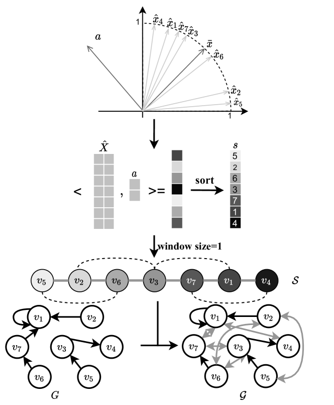
Figure 1. An illustration of the approximate similarity sorting. With the auxiliary vector $a$, we compute the cosine similarity between all node features $\hat{X}$ and the auxiliary vector $a$ to obtain a similarity score vector. Then, we sort the similarity scores in ascending or descending order, and return a sorted node index vector $s$. We connect the nodes in order according to the score ranking in the $s$ to generate a similarity sorting graph $\mathcal{S}$. Note that $\mathcal{S}$ is an undirected strongly connected graph, so $\mathcal{S}$ is irreducible. At last, we combine $\mathcal{S}$ and the input graph $G$ by adding all undirected edges in $\mathcal{S}$ to $G$ (grey double-directional arrow), to generate an irreducible graph $\mathcal{G}$.

The similarity sorting graph $\mathcal{S}=(A_{s},X)$ represent that each node connects to it top-$k$ most similar nodes, where $k=2=2window\_size$ in Figure 1. However, since we use one auxiliary vector, the similarity sorting is completely accurate only when $d=2$. Considering similar features are not mapped far away, we hence add skip connection edges on $\mathcal{S}$ and use the hyperparameter $window\_size$ to control the number of neighbors. $window\_size$ can be set to any positive integer, for example we show $window\_size=2$, i.e., $k=4$ by adding dummy line edges to $\mathcal{S}$ as shown in Figure 1. To guarantee sparsity, $k$ is usually set to a small value. The final combinatorial graph is denoted $\mathcal{G}=(\mathcal{A},X)$, where $\mathcal{A}=max(A,A_{s})$ is the element-wise maximum. The transition matrix of the combinatorial digraph $\mathcal{G}$ is $P_{fpr}=\mathcal{D}^{-1}\mathcal{A}$, where $\mathcal{D}$ is the diagonal degree matrix of $\mathcal{G}$. Performing random walk on $\mathcal{G}$ is called Feature-Aware PageRank, since in each step the walker has a possibility of teleporting to other nodes who have similar features to the current node. Compared with PageRank transition matrix $P_{pr}$, which uses all nodes as teleports, our Feature-Aware PageRank yields a sparse transition matrix while ensuring irreducibility. Besides, another necessary condition is aperiodicity. To satisfy it, we add a restart probability at each step of a random walk, i.e., jumping to the starting node, namely Personalized Feature-Aware PageRank (PFPR). Thus, the transition matrix of PFPR is $P_{pfpr}=\tilde{\mathcal{D}}^{-1}\tilde{\mathcal{A}}$, where $\tilde{\mathcal{A}}=\mathcal{A}+I$ and $\tilde{\mathcal{D}}_{ii}=\sum_{j}\tilde{\mathcal{A}}_{ij}$. Adding a self-loop for each node with a non-zero probability makes $\mathcal{G}$ aperiodic, because of the greatest common divisor of the lengths of its cycles is one.

The transition matrix $P_{pfpr}$ of PFPR is associated with an irreducible and aperiodic graph $\mathcal{G}$ with self-loops. According to Perron-Frobenius Theory (Poole, 2014) for non-negative matrix, $P_{pfpr}$ has a positive left eigenvector $\tilde{\pi}$ corresponding to its dominate eigenvalue 1 with algebraic multiplicity 1, which guarantees the random walk on $\mathcal{G}$ converge to a unique positive stationary distribution equal to $\tilde{\pi}$. Therefore, the Diglacian in eq. 2 can be rewritten as:

(4) $$\tilde{T}=\tilde{\Pi}(\tilde{\mathcal{D}}^{-1}-P_{pfpr}).$$

The remaining question is how to deal with the feature matrix $X$ with negative entries. We solve it by decomposing $X$ into $X=X^{+}+X^{-}$, where $X^{+}$ and $X^{-}$ only contain the positive and negative entries respectively. Based on $X^{+}$ and $X^{-}$, we will get two similarity sorting graphs and combine them into the original graph to construct $\mathcal{G}$.

3.3. DiglacianGCN

For an undirected graph, its Perron vector $\pi$ of transition matrix can be computed by $\pi_{i}=\frac{d_{i}}{\sum_{k}d_{k}}$, so the vector of node degrees $A\cdot e$ is a scalar multiple of $\pi$. Besides, since $\pi_{i}$ is the sum of all incoming probabilities from the neighbors of $v_{i}$ in a digraph, it hence plays the same role of degree vector in undirected graph that reflects the connectivity between nodes (Gleich, 2006). Based on these properties, (Chung, 2005) and (Zhou et al., 2005) define the normalized graph Laplacian as a Hermitian matrix by using $\Pi$ to normalize transition matrix instead of using the symmetrized adjacency matrix $A_{u}$. Following the same spirit, we define the augmented normalized Diglacian as:

(5) $$\mathcal{T}=\frac{1}{2}(\tilde{\Pi}^{\frac{1}{2}}(\tilde{\mathcal{D}}^{-1}-P_{pfpr})\tilde{\Pi}^{-\frac{1}{2}}+\tilde{\Pi}^{-\frac{1}{2}}(\tilde{\mathcal{D}}^{-1}-P_{pfpr}^{\top})\tilde{\Pi}^{\frac{1}{2}}),$$

which is a symmetric, real-valued Laplacian with a full set of real eigenvalues. Recall that GCN (Kipf and Welling, 2017) uses $1$-th order polynomials with specific coefficients to approximate the normalized graph Laplacian $D^{-\frac{1}{2}}(D-A)D^{-\frac{1}{2}}$ to $D^{-\frac{1}{2}}(D+A)D^{-\frac{1}{2}}$, which serves as a convolution support to do neighbor weighted aggregation for each node. Thus, following the same purpose, we can directly modify the augmented normalized Diglacian as:

(6) $$\hat{\mathcal{T}}=\frac{1}{2}(\tilde{\Pi}^{\frac{1}{2}}(\tilde{\mathcal{D}}^{-1}+P_{pfpr})\tilde{\Pi}^{-\frac{1}{2}}+\tilde{\Pi}^{-\frac{1}{2}}(\tilde{\mathcal{D}}^{-1}+P_{pfpr}^{\top})\tilde{\Pi}^{\frac{1}{2}})$$

The detailed spectral analysis can be found in Appendix A. Considering direction structure of the graph may be not always useful in some cases as stated in Section 1, we take the symmetrized adjacent matrix into consideration, so that the directionality of the graph can be learned. Hence, the $l$-th layer of DiglacianGCN is defined as:

(7) $$H^{(l)}=\sigma(H^{(l-1)}W_{0}^{(l)}+(\alpha\tilde{\mathcal{D}}_{u}^{-1}\mathcal{A}_{u}+\beta\hat{\mathcal{T}})H^{(l-1)}W_{1}^{(l)})$$

where $\sigma$ is the activation function, $W_{0}$ and $W_{1}$ the trainable matrix. Motivated by the good performance of MLP on some heterophilous graphs, we separate the self-embedding and its neighbor embedding, which is an effective design for networks with heterophily (Zhu et al., 2020b). We use $\tilde{\mathcal{D}}_{u}^{-1}\mathcal{A}_{u}$ and $\hat{\mathcal{T}}$ as the neighbor weighted matrices under undirected and directed setting respectively, and $\alpha,\beta\in\mathbb{R}^{1}$ are trainable scalers to balance them to learn a ”soft” directionality. We employ power iteration (Poole, 2014) to approximate the stationary distribution $\tilde{\pi}$. Since $P_{pfpr}$ has at most $|E|+2Nk$ non-zero entries, the power iteration needs $\mathcal{O}(|\mathcal{E}|t)$ computational complexity using sparse-dense matrix multiplications, where $|\mathcal{E}|$ is the number of non-zero entries in $P_{pfpr}$ and $t$ is the number of iterations.

3.4. DiglacianGCN-CT

Based on the PFPR transition matrix, we can preserve the underlying long-distance correlation on the feature level when performing a random walk on the combinatorial graph $\mathcal{G}$. Further, we aim to explore long-distance correlation on the topology level, so that these two aspects can be taken into account simultaneously. Previous work (Klicpera et al., 2019a; Wu et al., 2019; Klicpera et al., 2019b) has considered node proximity based on the length of shortest path between nodes, that is, the fewer hops from $v_{i}$ to $v_{j}$, the higher proximity of $v_{j}$ to $v_{i}$. This however does not fully reflect the mutual relationship between nodes in the network. Thus, we define a measure of node proximity based on commute time.

For two nodes $v_{i}$ and $v_{j}$, the hitting time $\mathcal{H}_{ij}$ is the expected steps it takes for a random walk to travel from $v_{i}$ to $v_{j}$, and the commute time between them $\mathcal{C}_{ij}=\mathcal{H}_{ij}+\mathcal{H}_{ji}$ is defined as the expected time it takes a random walk from $v_{i}$ to $v_{j}$ and then back to $v_{i}$. The dissimilarity between adjacent nodes leads to the heterophily of the graph, so we impose a stronger restriction on node proximity based on the commute times of the graph, i.e., if $v_{i}$ has a high probability of returning to itself via $v_{j}$ in a random walk, then $v_{i}$ and $v_{j}$ have high proximity. To preserve such proximity in the GNN model, we propose DiglacianGCN-CT, which defines the graph propagation matrix based on commute time.

By the results from the standard Markov chain theory (Aldous and Fill, 2002), we can calculate expected hitting times for random walks on any graph in terms of the fundamental matrix. Given a combinatorial digraph $\mathcal{G}$ with irreducible transition matrix $P_{pfpr}$ and stationary distribution $\tilde{\pi}$, the fundamental matrix $Z$ is defined as $Z=\sum^{\infty}_{t=0}(P_{pfpr}^{t}-e\tilde{\pi}^{\top})$. It is proved (Li and Zhang, 2012) that $Z$ converges to:

(8) $$Z=(I-P_{pfpr}+J\tilde{\Pi})^{-1}-J\tilde{\Pi},$$

where $J=ee^{\top}$ is an all-one matrix. Then the hitting time from $v_{i}$ to $v_{j}$ has the expression $H_{ij}=\frac{z_{jj}-z_{ij}}{\tilde{\pi}_{j}}$. We can derive its matrix form:

(9) $$\mathcal{H}=(Jdiag(Z)-Z)\tilde{\Pi}^{-1},$$

where $diag(Z)$ is the diagonal matrix formed by the main diagonal of $Z$. In eq. 8, the first term involves the inversion of a dense matrix, which has $\mathcal{O}(N^{3})$ time complexity. Based on our proposed Diglacian $T$ in eq. 2, we can compute $Z$ in a more efficient way.

Theorem 3.1.

Given a combinatorial digraph $\mathcal{G}$ and its Personalized Feature-Aware PageRank transition matrix $P_{pfpr}$, the Diglacian of $\mathcal{G}$ is defined as $\tilde{T}=\tilde{\Pi}(\tilde{\mathcal{D}}^{-1}-P_{pfpr})$. Then the fundamental matrix $Z$ of $\mathcal{G}$ can be solved by:

(10) $$Z=\tilde{\Pi}^{-\frac{1}{2}}(\tilde{\Pi}^{-\frac{1}{2}}\tilde{T}\tilde{\Pi}^{-\frac{1}{2}}-\tilde{\mathcal{D}}^{-1}+I)^{\dagger}\tilde{\Pi}^{\frac{1}{2}},$$

where the superscript $\dagger$ means Moore–Penrose pseudoinverse of the matrix.

The proof is given in Appendix B. The pseudoinverse of the sparse matrix in eq. 10 can be calculated via low-rank SVD. In particular, we use ARPACK (Lehoucq et al., 1998), an iteration method based on the restarted Lanczos algorithm, as an eigensolver. ARPACK depends on matrix-vector multiplication. Usually a small number of iterations is enough, so if the matrix is sparse and the matrix-vector multiplication can be done in $\mathcal{O}(N)$ time parallelly, then the eigenvalues are found in $\mathcal{O}(N)$ time as well.

Based on the fundamental matrix defined in eq. 10, we can compute the hitting time matrix $\mathcal{H}$ by eq. 9. The commute time matrix can be obtained by $\mathcal{C}=\mathcal{H}+\mathcal{H}^{\top}$, and we set $\mathcal{C}_{ii}=0$ for $i=1,\cdots,N$. Intuitively, the fewer steps a random walk takes to go from $v_{i}$ to $v_{j}$ and then returns to $v_{i}$, the higher the importance of $v_{j}$ to $v_{i}$. Also, since $\mathcal{G}$ is irreducible, all entries in $\mathcal{C}$ is positive, which yields a fully connected symmetric graph. It makes the subsequent propagation step computationally expensive and makes little sense for most downstream tasks. Hence, we sparsify $\mathcal{C}$ with a certain ratio $\mu\in(0,1)$. For each row of $\mathcal{C}$, we set $\mu N$ largest entries to 0. In doing so, we obtain a sparse non-negative matrix $\mathfrak{C}$. Then, we define the normalized graph propagation matrix based on $\mathfrak{C}$ as:

(11) $$\tilde{\mathfrak{C}}=\mathcal{D}_{s}^{-1}\exp(-\mathfrak{C}^{+}).$$

where $\mathfrak{C}^{+}$ means positive entires in $\mathfrak{C}$, $\mathcal{D}_{s}$ a diagonal matrix, $[\mathcal{D}_{s}]_{ii}=\sum_{j}[\exp(-\mathfrak{C}^{+})]_{ij}$. $\tilde{\mathfrak{C}}$ is the probability of a node moving to others based on the commute time of a random walk. Since the commute time matrix $\mathcal{C}$ is based on the Diglacian $\tilde{T}$ of the combinatorial graph $\mathcal{G}$, $\mathfrak{C}$ is also feature-aware. We replace $\tilde{\mathcal{T}}$ in eq. 7 with $\tilde{\mathfrak{C}}$ and define the $l$-th layer of DiglacianGCN-CT as:

(12) $$H^{(l)}=\sigma(H^{(l-1)}W_{0}^{(l)}+(\alpha\mathcal{D}_{u}^{-1}\mathcal{A}_{u}+\beta\tilde{\mathfrak{C}})H^{(l-1)}W_{1}^{(l)}),$$

where $\alpha$ and $\beta$ are trainable scalers.

Prediction. The class prediction $\hat{\mathbf{Y}}$ of a $L$-layer DiglacianGCN or DiglacianGCN-CT is based on node embeddings in the last layer:

(13) $$\hat{\mathbf{Y}}=\mathrm{softmax}(H^{(L)}),$$

where $W_{0}^{(L)},W_{1}^{(L)}\in\mathbb{R}^{d^{(L-1)}\times m}$, $d^{(L-1)}$ the dimension of the $(L-1)$-th layer and $m$ the number of classes.

3.5. Time Complexity

In the stage of constructing the combinatorial graph $\mathcal{G}$, the time complexity of the approximate similarity sorting including cosine similarity computation $\mathcal{O}(N)$ and similarity sorting $\mathcal{O}(N\log N)$. Then we compute the stationary distribution $\tilde{\pi}$ using power iteration, whose time complexity is $\mathcal{O}(tN)$, where $t\ll N$ is usually small. The total time complexity of an $L$-layer DiglacianGCN is therefore $\mathcal{O}(N\log N+LNd^{2})$. Further, the time complexity of computing the hitting matrix by the fundamental matrix based on eq. 10 is $\mathcal{O}(N)$. The time complexity of row-wise sparsification of $\mathfrak{C}$ is $\mathcal{O}(N\log N)$. In total, the DiglacianGCN-CT has the same time complexity as DiglacianGCN.

4. Experiments

4.1. Datasets

We conduct experiments on seven disassortative graph datasets and three assortative graph datasets, which are widely used in previous work. Specifically, the disassortative datasets including three web page graphs from the WebKB dataset (Pei et al., 2019) (Texas, Wisconsin and Cornell), three webpage graphs from Wikipedia (Pei et al., 2019) (Actor, Chameleon and Squirrel) and a social network of European Deezer (Lim et al., 2021) (deezer). On the other hand, the assortative datasets including two citation networks (CoraML (Bojchevski and Günnemann, 2018) and Citeseer (Frasca et al., 2020)) and a coauthor network (CoauthorCS (Shchur et al., 2018)). In order to distinguish assortative and disassortative graph datasets, Zhu et al. (2020b) propose the edge homophily ratio as a metric to measure the homophily of a graph $h=\frac{|\{(v_{i},v_{j})\in E:y_{i}=y_{j}\}|}{|E|}$, where $y_{i}$ is the label of $v_{i}$. This metric is defined as the proportion of edges that connect two nodes of the same class. The datasets that we used have edge homophily ratio ranging from low to high.

For all disassortative datasets except deezer, we use the feature vectors, class labels, and 10 fixed splits (48%/32%/20% of nodes per class for train/validation/test) from (Pei et al., 2019). For deezer, we use 5 fixed splits (50%/25%/25% for train/validation/test) provided by (Lim et al., 2021). For all assortative datasets, we use the same split as (Tong et al., 2020a), i.e., 20 labels per class for the training set, 500 labels for validation set and the rest for test set. The detailed information and statistics of these datasets are shown in Table 2.

Table 2. Statistics of the ten datasets used in our experiments.

Dataset $N$ $|E|$ # Feat. # Classes Digraph Texas 183 309 1,703 5 ✓ Wisconsin 251 499 1,703 5 ✓ Cornell 183 295 1,703 5 ✓ Chameleon 2,277 36,101 2,325 5 ✓ Squirrel 5,201 217,073 2,089 5 ✓ Actor 7,600 33,544 931 5 ✓ deezer 28,281 92,752 31,241 2 Cora-ML 2,995 8,416 2,879 7 ✓ Citeseer 3,312 4,715 3,703 6 ✓ CoauthorCS 18,333 81,894 6,805 15

Table 3. Classification accuracy (with standard deviation) in percent. The ”$*$” represents the best results among all variants of the model. For all baselines except MLP and ChebyNet, we respectively conduct experiments on symmetrized and original adjacency matrices and report the better results. Bold: best; Underline: runner-up.

Texas Wisconsin Actor Squirrel Chameleon Cornell deezer Citeseer CoraML CoauthorCS $h$ 0.11 0.21 0.22 0.22 0.23 0.3 0.53 0.74 0.79 0.81 MLP 81.89($\pm$4.78) 85.29($\pm$3.31) 35.76($\pm$0.98) 31.68($\pm$1.90) 46.21($\pm$2.99) 81.89($\pm$6.40) 66.55($\pm$0.72) 65.41($\pm$1.74) 77.12($\pm$0.96) 83.01($\pm$1.03) GCN 61.08($\pm$6.07) 53.14($\pm$5.29) 30.26($\pm$0.79) 52.43($\pm$2.01) 67.96($\pm$1.82) 61.93($\pm$3.67) 62.23($\pm$0.53) 66.03($\pm$1.88) 81.18($\pm$1.25) 91.33($\pm$0.45) GCN+r 71.08($\pm$5.41) 72.16($\pm$3.37) 33.72($\pm$0.95) 46.57($\pm$1.77) 58.35($\pm$1.89) 70.54($\pm$4.43) 60.37($\pm$2.01) 65.33($\pm$0.97) 68.31($\pm$2.12) 87.42($\pm$0.57) GCN+JK 69.19($\pm$6.53) 74.31($\pm$6.43) 34.18($\pm$0.85) 40.45($\pm$1.61) 63.42($\pm$2.00) 64.59($\pm$8.68) 60.99($\pm$0.14) 64.20($\pm$1.81) 80.16($\pm$0.87) 89.60($\pm$0.22) ChebyNet 79.22($\pm$7.51) 81.63($\pm$6.31) 28.27($\pm$1.99) 32.51($\pm$1.46) 59.17($\pm$1.89) 79.84($\pm$5.03) 67.02($\pm$0.59) 66.71($\pm$1.64) 80.03($\pm$1.82) 91.20($\pm$0.40) GAT 58.92($\pm$5.10) 61.37($\pm$5.27) 26.28($\pm$1.73) 40.72($\pm$1.55) 60.69($\pm$1.95) 62.73($\pm$3.68) 61.09($\pm$0.77) 67.58($\pm$1.39) 80.41($\pm$1.77) 90.82($\pm$0.48) AdaGraphSAGE 84.83($\pm$6.51) 85.88($\pm$3.58) 34.36($\pm$0.62) 48.78($\pm$1.30) 60.89($\pm$1.10) 81.35($\pm$5.97) 64.21($\pm$0.82) 67.02($\pm$1.80) 81.63($\pm$1.84) 90.57($\pm$0.56) GraphSAGE 83.92($\pm$6.14) 85.07($\pm$5.56) 34.23($\pm$0.99) 41.61($\pm$0.74) 58.73($\pm$1.68) 80.09($\pm$6.29) 64.28($\pm$1.13) 66.81($\pm$1.38) 80.03($\pm$1.70) 90.15($\pm$1.03) APPNP 79.57($\pm$5.32) 81.29($\pm$2.57) 35.93($\pm$1.04) 51.91($\pm$0.56) 45.37($\pm$1.62) 70.96($\pm$8.66) 67.21($\pm$0.56) 66.90($\pm$1.82) 81.31($\pm$1.47) 87.24($\pm$1.06) MixHop 77.84($\pm$7.73) 75.88($\pm$4.90) 32.22($\pm$2.34) 43.80($\pm$1.48) 60.50($\pm$2.53) 73.51($\pm$6.34) 66.80($\pm$0.58) 56.09($\pm$2.08) 65.89($\pm$1.50) 88.97($\pm$1.04) FAGCN 82.43($\pm$6.89) 82.94($\pm$7.95) 34.87($\pm$1.25) 42.59($\pm$0.79) 55.22($\pm$3.19) 79.19($\pm$9.79) 65.88($\pm$0.31) 68.93($\pm$1.17) 84.00($\pm$1.05) 91.07($\pm$1.28) H₂GCN-1 84.86($\pm$6.77) 86.67($\pm$4.69) 35.86($\pm$1.03) 36.42($\pm$1.89) 57.11($\pm$1.58) 82.16($\pm$4.80) 67.49($\pm$1.18) 64.57($\pm$2.06) 80.66($\pm$0.97) 88.45($\pm$0.97) H₂GCN-2 82.16($\pm$5.28) 85.88($\pm$4.22) 35.62($\pm$1.30) 37.90($\pm$2.02) 59.39($\pm$1.98) 82.16($\pm$6.00) 65.04($\pm$0.73) 67.15($\pm$0.99) 78.33($\pm$1.29) 88.53($\pm$0.38) CPGNN* 82.63($\pm$6.88) 84.58($\pm$2.72) 35.76($\pm$0.92) 29.25($\pm$4.17) 65.17($\pm$3.17) 79.93($\pm$6.12) 58.26($\pm$0.71) 66.19($\pm$1.74) 81.02($\pm$0.77) 89.20($\pm$0.91) GPRGNN 84.43($\pm$4.10) 83.73($\pm$4.02) 33.94($\pm$0.95) 50.56($\pm$1.51) 66.31($\pm$2.05) 79.27($\pm$6.03) 66.90($\pm$0.50) 61.74($\pm$1.87) 73.31($\pm$1.37) 91.49($\pm$0.39) GCNII 77.57($\pm$3.83) 80.39($\pm$3.40) 34.52($\pm$1.23) 38.47($\pm$1.58) 63.86($\pm$3.04) 77.86($\pm$3.79) 66.18($\pm$0.93) 58.32($\pm$1.93) 64.72($\pm$2.85) 84.13($\pm$1.91) DGCN 71.53($\pm$7.22) 65.52($\pm$4.71) 33.74($\pm$0.25) 37.16($\pm$1.72) 50.77($\pm$3.31) 68.32($\pm$4.30) 62.11($\pm$2.14) 66.37($\pm$1.93) 78.36($\pm$1.41) 88.41($\pm$0.68) DiGCN 65.18($\pm$8.09) 60.06($\pm$3.82) 32.45($\pm$0.78) 34.76($\pm$1.24) 50.55($\pm$3.38) 67.75($\pm$6.11) 58.37($\pm$0.89) 63.77($\pm$2.27) 79.51($\pm$1.34) OOM DiGCN-IB 66.97($\pm$13.72) 64.19($\pm$7.01) 32.82($\pm$0.68) 33.44($\pm$2.07) 50.37($\pm$4.31) 65.01($\pm$10.33) 55.39($\pm$2.88) 64.99($\pm$1.72) 81.07($\pm$1.14) 91.09($\pm$0.32) DiglacianGCN 87.84($\pm$3.25) 86.86($\pm$4.21) 35.57($\pm$1.10) 54.58($\pm$2.30) 70.70($\pm$2.07) 85.41($\pm$5.56) 66.52($\pm$0.17) 68.97($\pm$1.38) 82.30($\pm$0.81) 91.87($\pm$0.75) DiglacianGCN-CT 86.52($\pm$3.66) 87.06($\pm$4.03) 36.10($\pm$1.02) 56.22($\pm$2.09) 71.33($\pm$1.48) 87.30($\pm$7.18) 66.90($\pm$0.56) 67.85($\pm$1.68) 81.82($\pm$0.64) 91.60($\pm$0.34)

4.2. Baselines

We compare our DiglacianGCN and DiglacianGCN-CT against 19 benchmark methods. The full list of methods are:

• Structure-independent: 2-layer MLP.

• General GNNs: GCN (Kipf and Welling, 2017), ChebyNet (Defferrard et al., 2016), GAT (Veličković et al., 2018), GraphSAGE (Mean aggregation) (Hamilton et al., 2017), APPNP (Klicpera et al., 2019a), and jumping knowledge networks (GCN+JK, GCN+r) (Xu et al., 2018), where GCN+r only integrates knowledge from the input features.

• Digraph GNNs: DGCN (Tong et al., 2020b), DiGCN and DiGCN-IB (Tong et al., 2020a).

• Non-homophilous GNNs: MixHop (Abu-El-Haija et al., 2019), H₂GCN-1/2 (Zhu et al., 2020b), FA
  GCN (Bo et al., 2021), CPGNN (Zhu et al., 2020a), GPRGNN (Chien et al., 2021), and GCNII (Ming Chen et al., 2020).

Besides, to evaluate the effectiveness of our proposed graph propagation matrices $\tilde{\mathcal{T}}$ in DiglacianGCN and $\tilde{\mathfrak{C}}$ in DiglacianGCN-CT, we propose a variant of GraphSAGE, i.e., AdaGraphSAGE, as an additional baseline:

(14) $$H^{(l)}=\sigma(H^{(l-1)}W_{0}^{(l)}+(\alpha D_{u}^{-1}A_{u}+\beta D^{-1}A)H^{(l-1)}W_{1}^{(l)}).$$

For all baselines, we report their performance based on their official implementations after careful hyperparameter tuning.

4.3. Experimental Setting

For undirected graph datasets (deezer and CoauthorCS), i.e., all edges are bidirectional in the provided raw data, we directly use the original adjacency matrix in all baselines. In the experiments of digraph datasets, for ChebyNet as a spectral method, we use the symmetrized adjacency matrix. For other baselines, we apply both the symmetrized and asymmetric adjacency matrix for node classification. The results reported are the better of the two results. Note that GCN is a spectral method, but it can be interpreted from the spatial perspective, i.e., outgoing neighbor aggregation with specific weights $\frac{1}{\sqrt{d_{i}d_{j}}}$. Hence, we view GCN as a spatial method. Other implementation details including running environment, hyperparameter settings and corresponding search space are presented in Appendix C.

4.4. Node Classification

Table 3 reports the results of node classification on all ten graph datasets. We can see that our method DiglacianGCN and DiglacianG
CN-CT achieve new state-of-the-art results on 8 out of 10 datasets, and comparable results on two other datasets. Specifically, on datasets with strong heterophily ($h<0.5$), DiglacianGCN-CT achieves the best results on 5 out of 6 datasets and DiglacianGCN achieves the best result on 1 dataset and second-best results on 4 datasets. In particular, on Texas, Squirrel, Chameleon and Cornell, we achieve 87.84%, 54.22%, 71.33% and 87.30% accuracies respectively, which are 2.98%, 3.79%, 3.37% and 5.14% relative improvements over previous state-of-the-art. This demonstrates that considering the direction of edges can help the target nodes aggregate useful information, and commute time is an effective weighting scheme to help preserve long-distance dependency between nodes. On the dataset with intermediate heterophily ($h\approx 0.5$), our methods are competitive. Specifically, on deezer, H₂GCN and APPNP achieve the top two results, and DiglacianGCN-CT is the third. Our methods still have strong adaptability to homophilous graphs ($h>0.7$). Specifically, DiglacianGCN achieves the best results on Citeseer and CoauthorCS, and the second-best result on CoraML. DiglacianGCN-CT is the second-best on CoauthorCS and the third on CoraML. In addition, AdaGraphSAGE outperforms GraphSAGE in almost all datasets, that demonstrates adaptively learning the directionality of the graph is useful.

4.5. Adversarial Defense

Adversarial attacks on graphs aim to introduce minor modifications to the graph structure or node features that lead to a significant drop in the performance of GNNs. Recall that our methods provide two strategies, which are considering direction structure of the graph and underlying long-distance correlations between nodes, to greatly improve the performance on node classification tasks when graph structure is not reliable. This motivates us to examine the potential benefit of our models on adversarial defense. In this paper, we focus on perturbing the structure by adding or deleting edges, and evaluating the robustness of our methods on the node classification task. Specifically, we use metattack (Zügner and Günnemann, 2019) to perform non-targeted attack, and follow the same experimental setting as (Jin et al., 2021), i.e., the ratio of changed edges, from 0 to 25% with a step of 5%. We use GCN, GAT, APPNP and FAGCN as baselines and use the default hyperparameter settings in the authors’ implementations. The hyperparameter of our methods are the same with Section 4.4. We conduct the experiments on CoraML, Citeseer and Chameleon and report results in Figure 2.

From Figure 2a and Figure 2b, we can observe that all methods have similar downward trends. On Citeseer, APPNP and our DiglacianGCN achieve the best defensive effect under 5%$\sim$15% perturbation rate. FAGCN and APPNP achieve the best results under 20% and 25% perturbation rates respectively. On CoraML, DiglacianGCN achieves the best results under 10%$\sim$20% perturbation rate, and shows comparable performance to FAGCN under 5% and 25%. We can find that the class labels of CoraML are highly related to node feature according to the results of MLP in Table 3, that is the reason that Feature-Aware PageRank can help improve the robustness of our methods. From Figure 2c, we can find that DiglacianGCN-CT has more than 10% improvement over DiglacianGCN and other baselines under 15% perturbation rate, which demonstrates that the strategy of considering node proximity based on commute times can boost model robustness on heterophilous graphs.

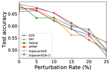
(a) Citeseer

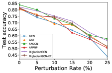
(b) CoraML

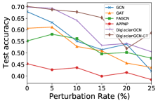
(c) Chameleon

Figure 2. Node classification performance under structural attack.

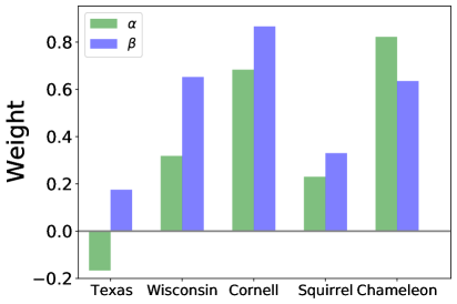
(a) DiglacianGCN

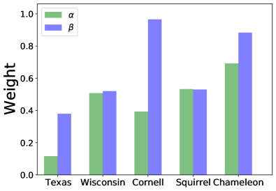
(b) DiglacianGCN-CT

Figure 3. Values of $\alpha$ and $\beta$ when the validation set achieve the best accuracy.

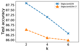
(a) Texas

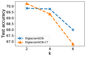
(b) Chameleon

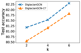
(c) CoraML

Figure 4. Node classification performance under different values of $k$.

4.6. Component Analysis

Directed v.s. Undirected. To verify the importance of considering the direction structure, we compare values of the learnable parameters $\alpha$ and $\beta$ in DiglacianGCN and DiglacianGCN-CT when achieving the best average accuracy on the validation set. It can reflect the tendency of directionality and the influence of direction structure on the classification accuracy on the testing set. As shown in Figure 4, we observe that the learned $\alpha$ and $\beta$ vary across different datasets, and in most cases our proposed graph propagation matrices $\tilde{\mathcal{T}}$ and $\tilde{\mathfrak{C}}$ have greater contributions to the final representations than that based on the symmetrized adjacency matrix. In addition, the results of AdaGraphSAGE and GraphSAGE in Table 3 indicate that instead of treating the given graph as a directed or undirected graph before training, adaptively learning the ”soft” directionality of the graph can improve the performance of models.

Feature-Aware PageRank v.s. PageRank v.s. $k$NN. In our models, we propose to construct a combinatorial graph $\mathcal{G}$ based on Feature-Aware PageRank to guarantee the irreducibility and aperiodicity, so that the Diglacian can be defined. We directly use PageRank transition matrix $P_{pr}=\alpha P+(1-\alpha)\frac{ee^{\top}}{N}$ with self-loop for the same purpose, which yields a dense and feature-independent propagation matrix. Correspondingly, we replace $P_{pfpr}$, $\tilde{\Phi}$ in eq. 6 to $P_{pr}$ and its stationary distribution, and $\tilde{\mathcal{D}}$ is replaced with the out-degree matrix of the original graph. We use ”(w/o feat.)” to represent this variant. This variant can help us verify the effectiveness of considering underlying correlations on the feature level. In addition, our methods are based on the preprocessed $\mathcal{G}$, where each node has additional edges to link to several non-neighbor nodes with similar features. The measure of feature similarity is based on the proposed approximate similarity sorting. Although it is not completely accurate, we can apply it to construct an irreducible graph efficiently. Hence, we compare it with accurate $k$NN. Since the $k$NN graph is not necessarily irreducible, we first construct a $k$NN graph based on node features $X$ and combine it to the original graph with self-loop to generate a combinatorial graph $\mathcal{G}^{kNN}$ where each node has additional edges linking to others with most similar features. Then, the PageRank transition matrix of $\mathcal{G}^{kNN}$ is irreducible, aperiodic, dense and feature-aware. We apply this transition matrix to DiglaicanGCN and DiglacianGCN-CT, and call this variant ”(w/ $k$NN)”. Besides, we record the average running time and GPU memory cost on each dataset and report the results in table 4. Results show that feature-independent variants are suboptimal. Although combining $k$NN graph can improve performance in some cases, it yields a fully connected combinatorial graph, significantly increasing the memory footprint. Besides, computing precise $k$NN is highly time-consuming.

Table 4. Comparison of our methods and their variants in average running time(s) and GPU memory cost(GB).

Texas Chameleon CoraML DiglacianGCN(w/o feat.) 84.33(15.3s/1.45GB) 62.57(183.3s/2.53GB) 79.59(82.8s/2.87GB) DiglacianGCN-CT(w/o feat.) 84.79(17.0s/1.84GB) 60.84(200.3s/2.39GB) 78.57(92.0s/2.45GB) DiglacianGCN(w/ $k$NN) 88.76(16.2s/1.45GB) 70.85(225.8s/2.53GB) 82.93(87.8s/2.87GB) DiglacianGCN-CT(w/ $k$NN) 86.97(18.9s/1.83GB) 71.26(237.0s/2.39GB) 81.86(97.5s/2.45GB) DiglacianGCN 87.84(8.8s/0.99GB) 70.70(148.3s/1.43GB) 82.30(77.8s/1.49GB) DiglacianGCN-CT 86.52(10.6s/0.97GB) 71.33(178.8s/1.45GB) 81.82(91.3s/1.47GB)

Parameter Sensitivity. In Section 3.2, we introduce the similarity sorting to generate an irreducible graph $S$ and then combine $S$ with the original graph $G$ to construct an irreducible combinatorial graph $\mathcal{G}$, where $k$ is set to a small value to guarantee sparsity. Hence, we explore the effect of $k$ on the performance of node classification task. We choose $k$ from $\{2,4,6\}$ and conduct experiments with different $k$ on 3 datasets, and report results in Figure 4. We find that the performance under different $k$ value is highly related to the results of MLP in Table 3. For example, on CoraML, MLP achieves not too bad classification accuracy, which indicates that the correlation between class labels and node features is high. In our models, with a larger $k$, nodes may gather more information from those with similar features, which makes nodes more discriminative. On the other hand, on Chameleon, MLP achieves a low accuracy, which means node features could mislead the node classification. Hence, a small $k$ is better in this dataset.

5. Conclusion

Our work aims to improve the performance of GNN on heterophilous graphs by considering direction structure and underlying long-distance correlations. We generalize the graph Laplacian to digraph by defining Diglacian based on the proposed Feature-aware PageRank, such that the direction structure and underlying feature-level long-distance correlations can be preserved simultaneously. The propagation matrix is based on the Diglacian and the symmetrized adjacency matrix such that the model can adaptively learn the directionality of the graph. Further, we define a measure of node proximity based on commute times and combine it into our model, which can capture the underly long-distance correlations between nodes on the topology level. The extensive experiments confirm the effectiveness and efficiency of our models.

Appendix A Spectral Convolution of the Diglacian

Since $P_{pfpr}\in\mathbb{R}^{N\times N}$ is a transition matrix of the combinatorial graph $\mathcal{G}$, following the inherent property of Markov chain (Poole, 2014), the eigenvalues $P_{pfpr}$ are bounded in $(-1,1]$. We first analyze the eigenvalues of $\mathcal{T}$. For clarity, we rewrite $\mathcal{T}$ in eq. 5 as:

(15) $$\mathcal{T}=\tilde{\mathcal{D}}^{-1}-\frac{1}{2}\left(\tilde{\Pi}^{\frac{1}{2}}P_{pfpr}\tilde{\Pi}^{-\frac{1}{2}}+\tilde{\Pi}^{-\frac{1}{2}}P_{pfpr}^{\top}\tilde{\Pi}^{\frac{1}{2}}\right).$$

Let $P_{pfpr}^{*}=\tilde{\Pi}^{\frac{1}{2}}P_{pfpr}\tilde{\Pi}^{-\frac{1}{2}}$, then $P_{pfpr}=\tilde{\Pi}^{-\frac{1}{2}}P_{pfpr}^{*}\tilde{\Pi}^{\frac{1}{2}}$. Let $\lambda$ denote a eigenvalue of $P_{pfpr}$ with the eigenvector $x$, i.e., $P_{pfpr}x=\lambda x$. Then, $\tilde{\Pi}^{-\frac{1}{2}}P_{pfpr}^{*}\tilde{\Pi}^{\frac{1}{2}}x=\lambda x$, and $P_{pfpr}^{*}\tilde{\Pi}^{\frac{1}{2}}x=\lambda\tilde{\Pi}^{\frac{1}{2}}x$. Therefore, eigenvalues of $P^{*}_{pfpr}$ are the same with $P_{pfpr}$ ranging in $(-1,1]$, with eigenvectors $\tilde{\Pi}^{\frac{1}{2}}x$. Thus, the eigenvalues $\lambda^{\mathcal{T}}$ of $\mathcal{T}$ is lower bounded by $\frac{1}{\tilde{d}_{max}}-1$ and upper bounded by $\frac{1}{\tilde{d}_{min}}+1$.

Since $\mathcal{T}$ is a real symmetric matrix, it has a complete set of orthonormal eigenvectors $\boldsymbol{U}=\left(\boldsymbol{u}_{1},\boldsymbol{u}_{2},\ldots,\boldsymbol{u}_{n}\right)$. Let $\boldsymbol{\Lambda}$ be a diagonal matrix of eigenvalues with $\boldsymbol{\Lambda}_{kk}=\lambda_{k}$. Since $\boldsymbol{U}$ is unitary, taking the eigenvectors of $\mathcal{T}$ as a set of bases, graph Fourier transform of a signal $f\in\mathbb{R}^{N}$ on graph $\mathcal{G}$ is defined as $\hat{f}=\boldsymbol{U}^{\top}f$, so the inverse graph Fourier transform is:

(16) $$f=\boldsymbol{U}^{\top}\hat{f}=\sum^{N}_{k=1}\hat{f}(k)\boldsymbol{u}_{k}.$$

According to convolution theorem, convolution in Euclidean space corresponds to pointwise multiplication in the Fourier basis. Denoting with $g$ the convolution kernel, the convolution of $f$ with the filter $g$ in the Fourier domain can be defined by:

(17) $$f*g=\boldsymbol{U}\left(\left(\boldsymbol{U}^{\top}g\right)\odot\left(\boldsymbol{U}^{\top}f\right)\right),$$

where $\odot$ is the element-wise Hadamard product, and $*$ is the graph convolution operator. Since the filter $g$ is free, the vector $\boldsymbol{U}^{\top}g$ can be any vector. Thus, the filter can be replaced by a diagonal matrix $\boldsymbol{\Sigma}=diag(\boldsymbol{\theta})$ parameterized by $\boldsymbol{\theta}\in\mathbb{R}^{N}$. We can rewrite eq. 17 as $\boldsymbol{U}\boldsymbol{\Sigma}\boldsymbol{U}^{\top}f$.

To reduce the number of tranable parameters to prevent overfitting and avoid explicit diagonalization of the matrix $\mathcal{T}$. Following ChebyNet (Defferrard et al., 2016), which restricts spectral convolution kernel $\boldsymbol{\Sigma}$ to a polynomial expansion of $\boldsymbol{\Lambda}$ and approximates the graph spectral convolutions by a truncated expansion in terms of Chebyshev polynomials up to $K$-th order, we define a normalized eigenvalue matrix, with entries in $(-1,1)$, by $\tilde{\boldsymbol{\Lambda}}=\frac{\boldsymbol{\Lambda}-\tilde{\mathcal{D}}^{-1}}{2}$, which can be verified by $\frac{1}{\tilde{d}_{max}}-1\leq\lambda^{\mathcal{T}}\leq\frac{1}{\tilde{d}_{min}}+1$. Then the graph convolution can be approximated by

(18) $$\boldsymbol{U}\Sigma\boldsymbol{U}^{T}f\approx\sum_{k=0}^{K}\theta_{k}T_{k}\left(\frac{\mathcal{T}-\tilde{\mathcal{D}}^{-1}}{2}\right)f,$$

where $T_{k}(\cdot)$ is the kth order matrix Chebyshev polynomial defined by $T_{0}(x)=1$, $T_{1}(x)=x$, and $T_{k}(x)=2xT_{k-1}(x)+T_{k-2}(x)$ for $k\geq 2$, $\theta_{0},\cdots,\theta_{k}$ real-valued parameters. Let $\boldsymbol{Y}=\boldsymbol{U}\Sigma\boldsymbol{U}^{T}$, we employ an affine appoximation ($K=1$) with coefficients $\theta_{0}=\theta$ and $\theta_{1}=2\theta$, from which we attain the graph convolution operation:

(19) $$\boldsymbol{Y}f\approx\theta\left(I+\frac{1}{2}\left(\tilde{\Pi}^{\frac{1}{2}}P_{pfpr}\tilde{\Pi}^{-\frac{1}{2}}+\tilde{\Pi}^{-\frac{1}{2}}P_{pfpr}^{\top}\tilde{\Pi}^{\frac{1}{2}}\right)\right)f$$

In our final form, we replace identity matrix $I$ in eq. 19 with $\tilde{\mathcal{D}}^{-1}$ as shown in eq. 6. The reason is that in eq. 19 the transition matrix is $P_{pfpr}+I$, which is equivalent to giving each node a large probability to move to itself in a random walk on $\mathcal{G}$. It makes the model hard to capture enough information from neighbors. Hence, we assume that the probability of the node moving to itself is the same as moving to its neighbors in each step, and it can be satisfied by eq. 6.

Appendix B Proof of Theorem 3.1

Proof.

As $P_{pfpr}^{t}J=J$, we have $ZJ=\boldsymbol{0}_{n\times n}$. Let $\mathfrak{T}=\tilde{\Pi}^{-\frac{1}{2}}\tilde{T}\tilde{\Pi}^{-\frac{1}{2}}=\tilde{\Pi}^{\frac{1}{2}}(\tilde{\mathcal{D}}^{-1}-P_{pfpr})\tilde{\Pi}^{-\frac{1}{2}}$, $\mathcal{J}=\tilde{\Pi}^{\frac{1}{2}}J\tilde{\Pi}^{\frac{1}{2}}$ and $\mathcal{Z}=\tilde{\Pi}^{\frac{1}{2}}Z\tilde{\Pi}^{-\frac{1}{2}}$, from eq. 8 we have:

(20) $$\mathcal{Z}+\mathcal{J}=(\mathfrak{T}+\mathcal{J}-\tilde{\mathcal{D}}^{-1}+I)^{-1},$$

then multiplying from the right by $(\mathfrak{T}+\mathcal{J}-\tilde{\mathcal{D}}^{-1}+I)$, we have:

(21) $$I =(\mathcal{Z}+\mathcal{J})(\mathfrak{T}+\mathcal{J}-\tilde{\mathcal{D}}^{-1}+I)$$

$$=\mathcal{Z}\mathfrak{T}+\mathcal{Z}\mathcal{J}-\mathcal{Z}\tilde{\mathcal{D}}^{-1}+\mathcal{Z}+\mathcal{J}\mathfrak{T}+\mathcal{J}^{2}-\mathcal{J}\tilde{\mathcal{D}}^{-1}+\mathcal{J}.$$

Since $\mathcal{J}^{2}=\mathcal{J}$, $\mathcal{J}\mathfrak{T}=\mathcal{J}(\tilde{\mathcal{D}}^{-1}-I)$, and $\mathcal{Z}\mathcal{J}=\tilde{\Pi}^{\frac{1}{2}}ZJ\tilde{\Pi}^{\frac{1}{2}}=\boldsymbol{0}_{n\times n}$, eq. 21 can be simplified to:

(22) $$\mathcal{Z}(\mathfrak{T}-\tilde{\mathcal{D}}^{-1}+I)=I-\mathcal{J}$$

Similarly, multiplying from the left we have $(\mathfrak{T}-\tilde{\mathcal{D}}^{-1}+I)\mathcal{Z}=I-\mathcal{J}$. As $\mathcal{\pi}^{\top}Z=\boldsymbol{0}$, we have $\mathcal{J}\mathcal{Z}=0$. Thus, $\mathcal{Z}(\mathfrak{T}-\tilde{\mathcal{D}}^{-1}+I)\mathcal{Z}=\mathcal{Z}$. Furthermore, it is easy to derive that $(\mathfrak{T}-\tilde{\mathcal{D}}^{-1}+I)\mathcal{J}=0$, then have $(\mathfrak{T}-\tilde{\mathcal{D}}^{-1}+I)\mathcal{Z}(\mathfrak{T}-\tilde{\mathcal{D}}^{-1}+I)=(\mathfrak{T}-\tilde{\mathcal{D}}^{-1}+I)$. Besides, the left part of eq. 22 symmetric, so $(\mathcal{Z}(\mathfrak{T}-\tilde{\mathcal{D}}^{-1}+I))^{\top}=\mathcal{Z}(\mathfrak{T}-\tilde{\mathcal{D}}^{-1}+I)$. Similarly, $((\mathfrak{T}-\tilde{\mathcal{D}}^{-1}+I)\mathcal{Z})^{\top}=(\mathfrak{T}-\tilde{\mathcal{D}}^{-1}+I)\mathcal{Z}$. These facts satisfy the sufficient conditions of Moore–Penrose pseudoinverse, such that

(23) $$\mathcal{Z}=(\mathfrak{T}-\tilde{\mathcal{D}}^{-1}+I)^{\dagger}.$$

Finally, recovering $\mathcal{Z}$ and $\mathfrak{T}$, which concludes the proof. ∎

Appendix C Implementation Details

Hardware infrastructures.

The experiments are conducted on Linux servers installed with a NVIDIA Quadro RTX8000 GPU and ten Intel(R) Xeon(R) Silver 4210R CPUs.

Hyperparameter Specifications

All parameters of our DiglacianGCN and DiglacianGCN-CT are initialized with Glorot initialization (Glorot and Bengio, 2010), and trained using Adam optimizer (Kingma and Ba, 2014) with learning rate $lr$ selected from $\{0.01,0.005\}$. The activation function $\sigma$ is $\mathrm{ReLU}$. The $l_{2}$ weight decay is selected from $\{0,5e-4,8e-4,1e-3\}$, and the dropout rate (Srivastava et al., 2014) is selected from $\{0.5,0.6,0.7\}$. The hyperparameter $k$ of Feature-aware PageRank is set to a non-zero even number, which selected from $\{2,4,6\}$. The number of iterations $t$ of the power method to compute the stationary distribution $\pi$ is set to 30 for all datasets. The dimension of hidden layers is selected from $\{48,64,96\}$ for all datasets and the number of layers is set to 2 for all datasets. For DiglacianGCN-CT, we set $\mu$ to 0.97 for all datasets to ensure the sparsity of the graph propagation matrix. In addition, we use an early stopping strategy on accuracies on the validation nodes, with a patience 500 epochs. All dataset-specific hyperparameter configurations are summarized in Table 5.

Table 5. Hyperparameter specifications.

Dataset	$k$	$lr$	Weight decay	Hidden dimension	Dropout
Texas	2	0.01	8e-4	48	0.6
Wisconsin	4	0.01	1e-3	96	0.7
Actor	2	0.01	1e-3	64	0.5
Squirrel	2	0.005	5e-4	64	0.5
Chameleon	2	0.01	5e-4	64	0.5
Cornell	6	0.01	1e-3	64	0.5
deezer	2	0.01	5e-4	64	0.5
Citeseer	4	0.01	8e-4	64	0.5
CoraML	6	0.01	5e-4	96	0.5
CoauthorCS	2	0.01	5e-4	64	0.5

References

- (1)
- Abu-El-Haija et al. (2019) Sami Abu-El-Haija, Bryan Perozzi, Amol Kapoor, Nazanin Alipourfard, Kristina Lerman, Hrayr Harutyunyan, Greg Ver Steeg, and Aram Galstyan. 2019. Mixhop: Higher-order graph convolutional architectures via sparsified neighborhood mixing. In international conference on machine learning. PMLR, 21–29.
- Aldous and Fill (2002) David Aldous and Jim Fill. 2002. Reversible Markov chains and random walks on graphs.
- Bo et al. (2021) Deyu Bo, Xiao Wang, Chuan Shi, and Huawei Shen. 2021. Beyond Low-frequency Information in Graph Convolutional Networks. In AAAI. AAAI Press.
- Bojchevski and Günnemann (2018) Aleksandar Bojchevski and Stephan Günnemann. 2018. Deep Gaussian Embedding of Graphs: Unsupervised Inductive Learning via Ranking. In International Conference on Learning Representations. https://openreview.net/forum?id=r1ZdKJ-0W
- Chen et al. (2019) Zhengdao Chen, Lisha Li, and Joan Bruna. 2019. Supervised Community Detection with Line Graph Neural Networks. In International Conference on Learning Representations. https://openreview.net/forum?id=H1g0Z3A9Fm
- Chien et al. (2021) Eli Chien, Jianhao Peng, Pan Li, and Olgica Milenkovic. 2021. Adaptive Universal Generalized PageRank Graph Neural Network. In International Conference on Learning Representations. https://openreview.net/forum?id=n6jl7fLxrP
- Chung (2005) Fan Chung. 2005. Laplacians and the Cheeger inequality for directed graphs. Annals of Combinatorics 9, 1 (2005), 1–19.
- Defferrard et al. (2016) Michaël Defferrard, Xavier Bresson, and Pierre Vandergheynst. 2016. Convolutional neural networks on graphs with fast localized spectral filtering. Advances in neural information processing systems 29 (2016), 3844–3852.
- Dong et al. (2021) Yushun Dong, Kaize Ding, Brian Jalaian, Shuiwang Ji, and Jundong Li. 2021. Graph Neural Networks with Adaptive Frequency Response Filter. arXiv preprint arXiv:2104.12840 (2021).
- Frasca et al. (2020) Fabrizio Frasca, Emanuele Rossi, Davide Eynard, Ben Chamberlain, Michael Bronstein, and Federico Monti. 2020. Sign: Scalable inception graph neural networks. arXiv preprint arXiv:2004.11198 (2020).
- Gilmer et al. (2017) Justin Gilmer, Samuel S Schoenholz, Patrick F Riley, Oriol Vinyals, and George E Dahl. 2017. Neural message passing for quantum chemistry. In International conference on machine learning. PMLR, 1263–1272.
- Gleich (2006) David Gleich. 2006. Hierarchical directed spectral graph partitioning. Information Networks 443 (2006).
- Glorot and Bengio (2010) Xavier Glorot and Yoshua Bengio. 2010. Understanding the difficulty of training deep feedforward neural networks. In Proceedings of the thirteenth international conference on artificial intelligence and statistics. JMLR Workshop and Conference Proceedings, 249–256.
- Hamilton et al. (2017) William L Hamilton, Rex Ying, and Jure Leskovec. 2017. Inductive representation learning on large graphs. In Proceedings of the 31st International Conference on Neural Information Processing Systems. 1025–1035.
- Jin et al. (2021) Wei Jin, Tyler Derr, Yiqi Wang, Yao Ma, Zitao Liu, and Jiliang Tang. 2021. Node similarity preserving graph convolutional networks. In Proceedings of the 14th ACM International Conference on Web Search and Data Mining. 148–156.
- Kingma and Ba (2014) Diederik P Kingma and Jimmy Ba. 2014. Adam: A method for stochastic optimization. arXiv preprint arXiv:1412.6980 (2014).
- Kipf and Welling (2017) Thomas N. Kipf and Max Welling. 2017. Semi-Supervised Classification with Graph Convolutional Networks. In International Conference on Learning Representations (ICLR).
- Klicpera et al. (2019a) Johannes Klicpera, Aleksandar Bojchevski, and Stephan Günnemann. 2019a. Predict then Propagate: Graph Neural Networks meet Personalized PageRank. In International Conference on Learning Representations (ICLR).
- Klicpera et al. (2019b) Johannes Klicpera, Stefan Weißenberger, and Stephan Günnemann. 2019b. Diffusion Improves Graph Learning. In Conference on Neural Information Processing Systems (NeurIPS).
- Lehoucq et al. (1998) Richard B Lehoucq, Danny C Sorensen, and Chao Yang. 1998. ARPACK users’ guide: solution of large-scale eigenvalue problems with implicitly restarted Arnoldi methods. SIAM.
- Li et al. (2018) Q. Li, Z. Han, and X.-M. Wu. 2018. Deeper Insights into Graph Convolutional Networks for Semi-Supervised Learning. In The Thirty-Second AAAI Conference on Artificial Intelligence. AAAI.
- Li and Zhang (2012) Yanhua Li and Zhi-Li Zhang. 2012. Digraph laplacian and the degree of asymmetry. Internet Mathematics 8, 4 (2012), 381–401.
- Lim et al. (2021) Derek Lim, Xiuyu Li, Felix Hohne, and Ser-Nam Lim. 2021. New Benchmarks for Learning on Non-Homophilous Graphs. arXiv preprint arXiv:2104.01404 (2021).
- Ming Chen et al. (2020) Zhewei Wei Ming Chen, Bolin Ding Zengfeng Huang, and Yaliang Li. 2020. Simple and Deep Graph Convolutional Networks. (2020).
- Page et al. (1999) Lawrence Page, Sergey Brin, Rajeev Motwani, and Terry Winograd. 1999. The PageRank citation ranking: Bringing order to the web. Technical Report. Stanford InfoLab.
- Pei et al. (2019) Hongbin Pei, Bingzhe Wei, Kevin Chen-Chuan Chang, Yu Lei, and Bo Yang. 2019. Geom-GCN: Geometric Graph Convolutional Networks. In International Conference on Learning Representations.
- Poole (2014) David Poole. 2014. Linear algebra: A modern introduction. Cengage Learning.
- Qu et al. (2019) Meng Qu, Yoshua Bengio, and Jian Tang. 2019. Gmnn: Graph markov neural networks. In International conference on machine learning. PMLR, 5241–5250.
- Shchur et al. (2018) Oleksandr Shchur, Maximilian Mumme, Aleksandar Bojchevski, and Stephan Günnemann. 2018. Pitfalls of graph neural network evaluation. arXiv preprint arXiv:1811.05868 (2018).
- Srivastava et al. (2014) Nitish Srivastava, Geoffrey Hinton, Alex Krizhevsky, Ilya Sutskever, and Ruslan Salakhutdinov. 2014. Dropout: a simple way to prevent neural networks from overfitting. The journal of machine learning research 15, 1 (2014), 1929–1958.
- Tong et al. (2020a) Zekun Tong, Yuxuan Liang, Changsheng Sun, Xinke Li, David Rosenblum, and Andrew Lim. 2020a. Digraph inception convolutional networks. Advances in neural information processing systems 33 (2020).
- Tong et al. (2020b) Zekun Tong, Yuxuan Liang, Changsheng Sun, David S Rosenblum, and Andrew Lim. 2020b. Directed graph convolutional network. arXiv preprint arXiv:2004.13970 (2020).
- Veličković et al. (2018) Petar Veličković, Guillem Cucurull, Arantxa Casanova, Adriana Romero, Pietro Liò, and Yoshua Bengio. 2018. Graph Attention Networks. International Conference on Learning Representations (2018). https://openreview.net/forum?id=rJXMpikCZ accepted as poster.
- Wu et al. (2019) Felix Wu, Amauri Souza, Tianyi Zhang, Christopher Fifty, Tao Yu, and Kilian Weinberger. 2019. Simplifying graph convolutional networks. In International conference on machine learning. PMLR, 6861–6871.
- Xu et al. (2018) Keyulu Xu, Chengtao Li, Yonglong Tian, Tomohiro Sonobe, Ken-ichi Kawarabayashi, and Stefanie Jegelka. 2018. Representation learning on graphs with jumping knowledge networks. In International Conference on Machine Learning. PMLR, 5453–5462.
- Zhang and Chen (2018) Muhan Zhang and Yixin Chen. 2018. Link prediction based on graph neural networks. Advances in Neural Information Processing Systems 31 (2018), 5165–5175.
- Zhou et al. (2005) Dengyong Zhou, Jiayuan Huang, and Bernhard Schölkopf. 2005. Learning from labeled and unlabeled data on a directed graph. In Proceedings of the 22nd international conference on Machine learning. 1036–1043.
- Zhu et al. (2020a) Jiong Zhu, Ryan A Rossi, Anup Rao, Tung Mai, Nedim Lipka, Nesreen K Ahmed, and Danai Koutra. 2020a. Graph Neural Networks with Heterophily. arXiv preprint arXiv:2009.13566 (2020).
- Zhu et al. (2020b) Jiong Zhu, Yujun Yan, Lingxiao Zhao, Mark Heimann, Leman Akoglu, and Danai Koutra. 2020b. Beyond Homophily in Graph Neural Networks: Current Limitations and Effective Designs. Advances in Neural Information Processing Systems 33 (2020).
- Zügner and Günnemann (2019) Daniel Zügner and Stephan Günnemann. 2019. Adversarial Attacks on Graph Neural Networks via Meta Learning. In International Conference on Learning Representations (ICLR).