Defeating Catastrophic Forgetting via Enhanced Orthogonal Weights Modification

Abstract

The ability of neural networks (NNs) to learn and remember multiple tasks sequentially is facing tough challenges in achieving general artificial intelligence due to their catastrophic forgetting (CF) issues. Fortunately, the latest OWM (Orthogonal Weights Modification) and other several continual learning (CL) methods suggest some promising ways to overcome the CF issue. However, none of existing CL methods explores the following three crucial questions for effectively overcoming the CF issue: that is, what knowledge does it contribute to the effective weights modification of the NN during its sequential tasks learning? When the data distribution of a new learning task changes corresponding to the previous learned tasks, should a uniform/specific weight modification strategy be adopted or not? what is the upper bound of the learningable tasks sequentially for a given CL method? ect. To achieve this, in this paper, we first reveals the fact that of the weight gradient of a new learning task is determined by both the input space of the new task and the weight space of the previous learned tasks sequentially. On this observation and the recursive least square optimal method, we propose a new efficient and effective continual learning method EOWM via enhanced OWM. And we have theoretically and definitively given the upper bound of the learningable tasks sequentially of our EOWM. Extensive experiments conducted on the benchmarks demonstrate that our EOWM is effectiveness and outperform all of the state-of-the-art CL baselines.

Introduction

Current state-of-the-art deep neural networks (NNs) can be trained to impressive performance on a wide variety of individual tasks (Krizhevsky, Sutskever, and Hinton 2017; LeCun, Bengio, and Hinton 2015; Huang et al. 2017). Learning multiple tasks in sequence, however, remains a substantial challenge in the NNs. When training on a new task, standard NNs will forget most of the information related to previously learned tasks, a phenomenon referred to as catastrophic forgetting (CF) (McCloskey and Cohen 1989; Chen and Liu 2018). Without solving this problem, the NN is hard to adapt to lifelong or continual learning(CL), which is crucial and fundamental for general artificial intelligence (GAI).

Problem Statement: Given a sequence of supervised learning tasks $T=(T_{1},T_{2},...,T_{N})$, we want to learn them one by one in the given sequence such that the learning of each new task will not forget the models learned for the previous tasks (Chen and Liu 2018; Hu et al. 2019).

For the CL research, there have been two main directions over the past 30 years, i.e., one from biological aspects, and the other from deep learning(Parisi et al. 2019). In this study, we focus on the latter. In recent years, many CL methods have been proposed to lessen the effect of CF (Hu et al. 2019; Parisi et al. 2019), e.g., learning without forgetting (LWF) (Li and Hoiem 2016), elastic weight consolidation (EWC) (Kirkpatrick et al. 2016), synaptic intelligence (SI)(Zenke, Poole, and Ganguli 2017), dynamically expandable network (DEN) (Yoon et al. 2018), progressive neural networks (PNN) (Rusu et al. 2016), averaged gradient episodic memory (AGEM) (Chaudhry et al. 2019), parameter generation and model adaptation (PGMA) (Hu et al. 2019), learn to grow (LTG) (Li et al. 2019), maximally interfered retrieval(MIR) (Aljundi et al. 2019), online fast adaptation and knowledge accumulation (OSAKA) (Caccia et al. 2020), etc. Despite the advantages of the above CL methods, however, none of the above existing CL methods explores the following three crucial questions for effectively overcoming the CF issue: such as, what knowledge does it contribute to the effective weights modification of the NN during its sequential tasks learning? When the data distribution of a new learning task changes corresponding to the previous learned tasks, should a uniform/specific weight modification strategy be adopted or not? what is the upper bound of the learningable tasks sequentially for a given CL method? According to whether task identity is provided and whether it must be inferred during test, there are mainly three CL scenarios (Hsu, Liu, and Kira 2018; van de Ven and Tolias 2019), i.e., task incremental learning, domain incremental learning and class incremental learning (CIL). CIL is the most challenging scenario in which the classes of each task are assumption of joint or disjoint and the model is trained to distinguish classes of all tasks with a shared output layer, namely single-head. Among the existing CL algorithms, it is worth mentioning that OWM (Orthogonal Weights Modification) algorithm (Zeng et al. 2019) and its few variants (He and Jaeger 2018; Shen et al. 2020; Farajtabar et al. 2020; Bennani and Sugiyama 2020), heareafter abbreviated as OWM algorithms, emerged in recent years are suggested to be a promising solution to the CIL scenario as their excellent theory, interpretability and performance (Hsu, Liu, and Kira 2018; van de Ven and Tolias 2019; Zeng et al. 2019). In the OWM algorithms, a good OWM projector $P_{OWM}$, which uses to find a gradient orthogonal direction, is the key of its method performance. Although the above latest few OWM algorithms have achieved gratifying results, however, we found that the existing OWM algorithms have following weaknesses: 1) none of their $P_{OWM}$ adopt all the necessary knowledge, 2) they make an unpractical assumption of being disjoint between classes of sequential tasks, and 3) they have considerably less attention to the rigorous evaluation of the algorithms. In this study, aiming to achieve all of the above weaknesseswe of OWM and above representative CL algorithms, we propose a new improved enhanced OWM algorithm, namely EOWM (Enhanced Orthogonal Weights Modification) . Our contributions can be summarized as follows:

• We theoretically study the projector $P_{OWM}$ of the existing OWM algorithms, andwe first reveals the fact that of the weight gradient of a new learning task is determined by both the input space of the new task and the weight space of the previous learned tasks sequentially. On the basis, we propose an enhanced projector $P_{EOWM}$, which can achieve all the above weaknesses of exsiting OWM and other CL algorithms.

• Based on our proposed $P_{EOWM}$ and the recursive least square optimal method, we present a new efficient enhanced OWM algorithm EOWM followed by introducing a more reasonable metric to address the weakness of considerably less attention to the rigorous evaluation of the OWM algorithms.

• Extensive experiments conducted on benchmark datasets show that our proposed algorithm EOWM achieves a new SOTA (State-Of-The-Art) results compared with some competitive baselines.

This paper is organized as follows. Section 2 first gives some preliminaries, and overviews related work. Section 3 details our theoretical study to the projector $P_{OWM}$ of the OWM methods followed by our proposed algorithm EOWM. Section 4 reports experimental results on benchmark datasets to evaluate our method. Finally, Section 5 concludes this study.

Related Work

In this study, as we focus on a new and enhanced OWM algorithm, which is expected to effectively overcome the above weaknesses of the existing CL and OWM algorithms, we first outline the OWM methods, and then overview the latest related OWM algorithms.

Preliminaries

OWM method: It is also called subspace methods (He and Jaeger 2018; Zeng et al. 2019). Its basic strategy used in these algorithms is that it retains previously learned knowledge by keeping the old input-output mappings that NNs induce fixed. To meet this goal, the gradients are projected to the subspace that is orthogonal to the inputs of past tasks. More formally, in OWM, a projector $P_{OWM}$ used to find the orthogonal direction to the input space is defined as (Zeng et al. 2019)

$$P_{OWM}=I-A_{n-1}\left(A_{n-1}^{T}A_{n-1}+\alpha I\right)^{-1}A_{n-1}^{T}$$ (1)

where $A_{n-1}$ consists of all $n-1$ previously trained input vectors as its columns $A_{n-1}$ = $(\boldsymbol{x_{1}},...,\boldsymbol{x_{n-1}})$, and $I$ is a $n-1$ order unit matrix multiplied with a relatively small constant $\alpha$. For the n-th new learning task, the learning-induced weights modification of a NN is then updated by the weight gradient, which is calculated according to the standard back-propagation and modified by the projector $P_{OWM}$ It is worth noting that a well-designed projector $P_{OWM}$ is the vital to a effective and efficient OWM algorithm.

Related work

Among a few OWM algrithms, OWM method (Zeng et al. 2019) is the pioneer of this kind of algorithms. Inspired by the role of the prefrontal cortex (PFC) in mediating context-dependent processing in the primate brain, the OWM first proposed a novel orthogonal weights modification method with the addition of a PFC-like module, that enables CNNs to continually learn different mapping rules in a context-dependent way without interference leading to reach a human level ability in online and continual learning.

CAB (He and Jaeger 2018) proposed a variant of the back-propagation algorithm based on OWM basic principle, i.e., conceptor-aided backprop (CAB), in which gradients are shielded by conceptors against degradation of previously learned tasks. On the benchmark datasets CAB outperforms its baselines for coping with catastrophic interference.

Inspired by the first OWM method (Zeng et al. 2019), (Shen et al. 2020) proposed an improve OWM method, namely OWM+GFR, with the strategy of directly generating and replaying features. its empirical results on image and text datasets showed that the OWM+GFR can improve OWM (Zeng et al. 2019) consistently by a significant margin while conventional generative replay always resulted in a negative effect, and beats a SOTA generative replay method (Hu et al. 2019).

From the parameter space perspective, OGD (Farajtabar et al. 2020) and OGD+ (Bennani and Sugiyama 2020) studied an approach to restrict the direction of the gradient updates to avoid forgetting previous-learned tasks, which accomplished its goal by projecting the gradients from new tasks onto a subspace where the neural network output on previous tasks do not change and the projected gradient is still in a useful direction. Moreover, OGD+ proved that OGD was robust to CF then derived the first generalization bound for SGD (Stochastic Gradient Descent) (Sinha and Griscik 1971) and OGD for CL.

Though the above few pioneering OWM algorithms claimed that they were the most promising solution to the CF problem, we suggest that they have three serious weaknesses (see Para. 5 of Introduction for details). Different from all of the above OWM methods, based on our findings we proposed a new enhanced OWM method, namely EOWM, to achieve all the above weaknesses of the existing OWM and other CL methods.

The Proposed Enhanced OWM

Basic Concepts

For clarity, based on optimization theory(Saad 2003), we first introduce following basic concepts and notations.

Definition 1: Weight Space. For a NN, let $W_{i}$ be the weight matrix of a layer learning the $i$-th task $T_{i}$ sequentially. And define $\Omega_{n-1}$ as the weight space of learned previous $n-1$ tasks, which consists of all $n-1$ previously weight matrices as its columns, i.e., $\Omega_{n-1}=(W_{1},W_{2},...,W_{n-1})$. And denote $\Omega_{n-1}^{\perp}$ as the orthogonal subspace of $\Omega_{n-1}$.

Given a NN, its weight matrix $W_{n}$ for the learning task $T_{n}$ can be calculated by the gradient descent method (Amari 1993) as follows.

$$W_{n}=W_{n-1}-\lambda\Delta W_{n}$$ (2)

where $\lambda$ is the learning rate and $\Delta W_{n}$ corresponds to the weight gradient for the task $T_{i}$.

Definition 2: Projections. Let $\Delta W_{n}^{\Omega_{n-1}}$($\Delta W_{n}^{\Omega_{n-1}^{\perp}}$) be the projections of $\Delta W_{n}$ on $\Omega_{n-1}$ ($\Omega_{n-1}^{\perp}$). From the basic definition of projection(Saad 2003), we have

$$\begin{cases}\Delta W_{n}=\Delta W_{n}^{\Omega_{n-1}}+\Delta W_{n}^{\Omega_{n-1}^{\perp}}\ \\ s.t.\ \Delta W_{n}^{\Omega_{n-1}}\in\Omega_{n-1},\ \Delta W_{n}^{\Omega_{n-1}^{\perp}}\in\Omega_{n-1}^{\perp}\end{cases}$$ (3)

Definition 3: Projection operator. Let $Q$ and $Q_{ort}$ be the projection operators that project $\Delta W_{n}$ to $\Omega_{n-1}$ and $\Omega_{n-1}^{\perp}$, respectively. Based on the basic definition of the projection operator(Gloub and Van Loan 1996; Saad 2003), $Q$ and $Q_{ort}$ can be computed as follows.

$${\begin{cases}Q=\Omega_{n-1}\left(\Omega_{n-1}^{T}\Omega_{n-1}+\beta I\right)^{-1}\Omega_{n-1}^{T}\ \\ Q_{ort}=I-\Omega_{n-1}\left(\Omega_{n-1}^{T}\Omega_{n-1}+\beta I\right)^{-1}\Omega_{n-1}^{T}\ \end{cases}}$$ (4)

where $\beta$ is a very small positive empirical constant.

On the above basis, following Eq.5 can be deduced.

$${\begin{cases}\Delta W_{n}^{\Omega_{n-1}}=\Delta W_{n}Q\ \\ \Delta W_{n}^{\Omega_{n-1}^{\perp}}=\Delta W_{n}Q_{ort}\ \\ \end{cases}}$$ (5)

Based on Eqs.3 to 5, following Theorems can be obtained.

Theorem 1: $\Delta W_{n}^{\Omega_{n-1}}$ and $\Delta W_{n}^{\Omega_{n-1}^{\perp}}$ only contain the knowledge of the previous learned tasks $(T_{1},T_{2},...,T_{n-1})$ and the current learning task $T_{n}$, respectively.

Proof: As $\Delta W_{n}^{\Omega_{n-1}}\in\Omega_{n-1}$ and $\Delta W_{n}^{\Omega_{n-1}^{\perp}}\in\Omega_{n-1}^{\perp}$, $\Delta W_{n}^{\Omega_{n-1}}$ only contains the knowledge of previous learned tasks. $\Omega_{n-1}^{\perp}$ is orthogonal to $\Omega_{n-1}$, so $\Delta W_{n}^{\Omega_{n-1}^{\perp}}$ only contains the knowledge of the new task $T_{n}$. $\hfill\blacksquare$

Theorem 2: When a NN learns a new task $T_{n}$, both the two projections $\Delta W_{n}^{\Omega_{n-1}}$ and $\Delta W_{n}^{\Omega_{n-1}^{\perp}}$ of the weight gradient $\Delta W_{n}$ of $T_{n}$ will disturb the weight space $\Omega_{n-1}$ of the previous learned tasks $(T_{1},T_{2},...,T_{n-1})$, and $\Omega_{n-1}$ would be transformed into a new weight space $\Omega_{n}$ as follows.

$$\Omega_{n}=\left[\Omega_{n-1},-\lambda\left(\Delta W_{n}^{\Omega_{n-1}}+\Delta W_{n}^{\Omega_{n-1}^{\perp}}\right)\right]$$ (6)

where $\Delta W_{n}^{\Omega_{n-1}}\in\Omega_{n-1}$, and $\Delta W_{n}^{\Omega_{n-1}^{\perp}}\not\in\Omega_{n-1}$.

Proof: After the new task $T_{n}$ with the weight matrix $W_{n}$ is trained, its weight space has changed as $\Omega_{n}=\left[W_{1},W_{2},...,W_{n-1},W_{n}\right]$.

With Eq.2, $\Omega_{n}=\left[W_{1},W_{2},...,W_{n-1},\left(W_{n-1}-\lambda\Delta W_{n}\right)\right]$. Following the equivalence of elementary transformation of matrix and Eq.3, we have

$$\ \ \ \ \ \ \ \ \ \ \ \ \ \ \ \ \ \ \ \ \ \ \ \ \ \ \ \ \ \ {\begin{aligned} \Omega_{n}&=\left[W_{1},W_{2},...,W_{n-1},-\lambda\Delta W_{n}\right]\\ &=\left[W_{1},W_{2},...,W_{n-1},-\lambda\left(\Delta W_{n}^{\Omega_{n-1}}+\Delta W_{n}^{\Omega_{n-1}^{\perp}}\right)\right]\\ &=\left[\Omega_{n-1},-\lambda\left(\Delta W_{n}^{\Omega_{n-1}}+\Delta W_{n}^{\Omega_{n-1}^{\perp}}\right)\right]\ \ \ \ \ \ \ \ \ \ \ \ \ \ \ \ \ \ \ \hfill\blacksquare\end{aligned}}$$

In particular, the above Theorems and Eq.6 clearly reveals the fact that the new weight space for the new task $T_{n}$ consists of two parts, where one is the previous learned weight space $\Omega_{n-1}$, and another is the influence of old knowledge ($\Delta W_{n}^{\Omega_{n-1}}$) and new knowledge ($\Delta W_{n}^{\Omega_{n-1}^{\perp}}$) on $\Omega_{n-1}$.

An Enhanced Projection Operator $P_{EOWM}$

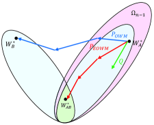
(a) The classes in task $T_{A}$ and task $T_{B}$ intersect, denoted as $T_{A}\simeq T_{B}$.

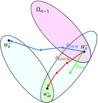
(b) The classes in task $T_{A}$ and task $T_{B}$ disjoint, denoted as $T_{A}\not\simeq T_{B}$.

Figure 1: The schematic diagram of moving trajectories of $P_{OWM}$ and proposed $P_{EOWM}$, where $W_{A}^{*}$ (pink area), $W_{B}^{*}$ (blue area) and $W_{AB}^{*}$ (green area) represent the optimal weights about task A, task B, and both task A and task B, respectively. Both Figs.(a) and (b) clearly indicate that $P_{EOWM}$ always progresses towards optimal direction $W_{AB}^{*}$ of both the previous learned task A and the new learning task B, while $P_{OWM}$ does towards the optimal direction $W_{B}^{*}$ of the new learning task B.

Equipped with the above revealed important fact, we aim to seek an enhanced projecting operator denoted as $P_{EOWM}$ to overcome the existing OWM and other CL methods’ weaknesses. For clarity, we first introduce Def.5 followed by our proposed $P_{EOWM}$. Definition 5: For simplicity, let the class label set of all the previous learned/trained tasks $T_{prev}$ as $C_{prev}$, while the class label set of new learned/trained task $T_{new}$ as $C_{new}$. If $C_{prev}\cap C_{new}\neq\varnothing$, we define that $T_{prev}$ is similar to or joints $T_{new}$ denoted as $T_{prev}\simeq T_{new}$. Otherwise, both $T_{pewv}$ and $T_{new}$ are dissimilar, namely disjoint denoted as $T_{prev}\not\simeq T_{new}$.

An Enhanced Projection Operator $P_{EOWM}$: In practice, the classes of sequentially learning tasks may be joint or disjoint. Considering the both situations, we calculate the $P_{EOWM}$ as follows:

1) if $T_{prev}\simeq T_{new}$, The weight space $\Omega_{n-1}$ of $T_{prev}$ most likely to contains optimal weights of the new task $T_{new}$. Based on the Def. 3 and Theorem 2, the correction matrix of the weight gradient of $T_{new}$, i.e., $P_{EOWM}$, should increase a gradient change over $\Omega_{n-1}$; Otherwise,

2) the optimal network weights to the new task $T_{new}$ on $\Omega_{n-1}^{\perp}$ should be ensured and enhanced. As $\Omega_{n-1}^{\perp}$ and $\Omega_{n-1}$ are orthogonal, the learning of the optimal network weights of $T_{new}$ will not affect the original network weights of the previous tasks $T_{prev}$.

Fig.1 illustrates the core idea of our $P_{EOWM}$, that is, $P_{EOWM}$ will always guide the weights gradient towards the optimal direction for previous learned tasks and new learning task. In short, our $P_{EOWM}$ can be formalized as follows:

$$P_{EOWM}=\begin{cases}P_{OWM}(c_{1}I+c_{2}Q),\ T_{prev}\simeq T_{new}\ \\ P_{OWM}(c_{1}I+c_{2}Q_{ort}),\ T_{prev}\not\simeq T_{new}\ \end{cases}$$ (7)

where $c_{1}$ and $c_{2}$ are positive empirical coefficients less than 1, and $c_{1}+c_{2}=1$. $Q$ and $Q_{ort}$ are the projection operators that project $\Delta W_{n}$ to $\Omega_{n-1}$ and $\Omega_{n-1}^{\perp}$, respectively (see Def.3 and Eq.4).

Let the correction matrix of the weight gradient for new task $T_{n}$ be $P_{EOWM}^{n}$. $P_{EOWM}^{n}$ is used to modify its weight gradient $\Delta W_{n}$, According to Eq.2, the weight of a new task $T_{n}$ can be updated by following Eq.8.

$${W_{n}=W_{n-1}-\lambda\Delta W_{n}P_{EOWM}^{n}\\ }$$ (8)

The efficient iterative calculation of $P_{EOWM}$: To avoid the heavy computation cost of large-scale matrix operations in Eqs.7 and 8, Based on the Recursive Least Square (RLS) algorithm(Shah, Palmieri, and Datum 1992), an efficient iterative calculation of $P_{EOWM}$ is carefully designed, which is shown in Theorem 3 for details..

Theorem 3: $P_{EOWM}$ can be calculated efficiently and iteratively by Eq.9 (proof shown in Appedix A).

$$P_{EOWM}^{n+1}=\begin{cases}P_{OWM}^{n+1}(c_{1}I+c_{2}Q^{n+1}),\ T_{prev}\simeq T_{n+1}\ \\ P_{OWM}^{n+1}(c_{1}I+c_{2}Q_{ort}^{n+1}),\ T_{prev}\not\simeq T_{n+1}\ \end{cases}$$ (9)

where $P_{OWM}^{n+1}=P_{OWM}^{n}-\boldsymbol{\kappa}_{x}\bar{\textbf{x}}_{n}^{T}P_{OWM}^{n}$, and $\boldsymbol{\kappa}_{x}=\left(\alpha+\bar{\textbf{x}}_{n}^{T}P_{OWM}^{n}\bar{\textbf{x}}_{n}\right)^{-1}P_{OWM}^{n}\bar{\textbf{x}}_{n}$. $\bar{\textbf{x}}_{n}$ corresponds to the mean value of task $T_{n}$’s input, and $\alpha$ is a small constant same as in Eq.2, respectively. The iterative equation of $Q_{ort}$ and $Q$ is given as follows.

$$\begin{cases}Q_{ort}^{n+1}&=Q_{ort}^{n}-\boldsymbol{\kappa}_{W}\overline{\textbf{W}}_{n}^{T}Q_{ort}^{n}\\ Q^{n+1}&=I-Q_{ort}^{n}\end{cases}$$ (10)

where $\boldsymbol{\kappa}_{W}=\left(\beta+\overline{\textbf{W}}_{n}^{T}Q_{ort}^{n}\overline{\textbf{W}}_{n}\right)^{-1}Q_{ort}^{n}\overline{\textbf{W}}_{n}$. $\overline{\textbf{W}}_{n}$ and $\beta$ are the mean value of network weights after task $T_{n}$ learned and the small constant in Eq.4, respectively.

Theorem 3 clearly indicates that the iterative computation of $P_{EOWM}$ only need the input of current learning task $T_{n}$ and its weight matrix $W_{n}$, which greatly reduces the storage space and speedup the calculation.

The proposed EOWM Algorithm

On the above basis, we present a novel enhanced OWM algorithm, namely EOWM. Its algorithm pseudo-code and training framework are shown in Alg.1 and Fig.2, respectively.

Algorithm 1 EOWM algorithm

Input: The sequential tasks $\{T_{1},T_{2},...,T_{N}\}$
Parameter: Regular terms $\alpha$ and $\beta$ of projection operator; Learning rate $\lambda$
Output: All tasks’ predicted labels $\bar{y}$

1:  Randomly initialize the neural network weights $W$, $P_{OWM}\leftarrow I/\alpha$, $Q_{ort}\leftarrow I/\beta$, $T_{prev}\leftarrow\text{\o}$, $\bar{y}$ $\leftarrow\text{\o}$;

2:  while each $j\in[1,$ $N]$ do

3:     $\bar{y}_{j}$ $\leftarrow\textbf{{Forward}}(x_{j})$; //$\bar{y}_{j}$ is the predicted label for $T_{j}$.

4:     $\Delta W_{j}\leftarrow\textbf{{Backward}}(\textbf{{Loss}}(y_{j}$, $\bar{y}_{j}$));

5:     if j = 1 then

6:        Calculate $W_{j}$ by Eq.2;

7:     else

8:        Calculate $W_{j}$ by Eq.8;// Update weights by $P_{EOWM}$.

9:     end if

10:     Calculate $P_{OWM}$ by Eq. 9;

11:     Calculate $Q_{ort}$ and $Q$ by Eq. 10;

12:     $sim=\textbf{{Similarity}}(T_{prev},T_{j})$;

13:     Calculate empirical coefficients $c_{1}$ and $c_{2}$ with $sim$

14:     Calculate $P_{EOWM}$ by Eq. 9;// Generate $P_{EOWM}$.

15:     $T_{prev}\leftarrow T_{prev}\cup T_{j}$;

16:     $\bar{y}$ $\leftarrow$ $\bar{y}$ $\cup$ $\bar{y_{j}}$;

17:  end while

18:  return $\bar{y}$.

The proposed EOWM algorithm consists of three functional modules: 1) initialization (shown in line 1 in Alg.1), 2) updating Weights of the $NN$ by $P_{EOWM}$ layer-by-layer (shown in lines 3 to 9 in Alg.1), with the forward propagation algorithm (Forward(·)), back propagation algorithm Backward(·), and Loss function (Loss(·)), respectively. Note that the weights updating for the Task $T_{1}$ is calculate by Eq.2, while for the other tasks $T_{2}...T_{N}$ by Eq.8, and 3) generating final weights of the $NN$ by Eqs.9 and 10 with similarity function (Similarity(·)) (shown in lines 10 to 16 in Alg.1).

The training pipeline of the EOWM is shown in Fig.2. In training for task $T_{n}$, the correction matrix $P_{EOWM}^{n}$ is firstly calculated based on $P_{EOWM}^{n-1}$ of the previous tasks $T_{prev}$ ($T_{1}...T_{n-1}$). Then the class labels of the task $T_{n}$ are predicted with forward propagation algorithm Forward(·). Finally, the training of current task $T_{n}$ is completed with the back propagation algorithm Backward(·).

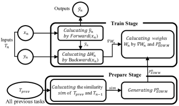
Figure 2: The training framework of our EOWM algorithm.

Especially noteworthy is that our proposed EOWM algorithm also has the following two unique properties (shown in Theorems 4 and 5) by our theoretical analysis and extensive experiments.

Theorem 4: The time complexity of our EOWM algorithm is $O(N_{c}^{3}N_{n})$, where $N_{c}$ and $N_{n}$ are the numbers of the columns of the weight and neurons of a layer in the NN, respectively (proof shown in Appedix B).

As the capacity of one layer of the $NN$ can be measured by the rank of $P_{EOWM}$, we can use the rank of $P_{EOWM}$, denoted as $rank(P_{EOWM})$, for the number of learnable different tasks(Zeng et al. 2019).

Theorem 5 : The upper bound of the minimum number of learnable tasks of our proposed EOWM is $rank(P_{EOWM})$, which is fomulated as follows.

$${rank(P_{EOWM})<=\begin{cases}Rank_{OWM}+rank(P_{OWM}Q),\ T_{prev}\simeq T_{n+1}\ \\ Rank_{OWM}+rank(P_{OWM}Q_{ort}),\ T_{prev}\not\simeq T_{n+1}\ \end{cases}}$$

where $Rank_{OWM}$ is the maximum rank of $P_{OWM}$ when $rank(P_{OWM}Q)>0$ and $rank(P_{OWM}Q_{ort})>0$ (proof shown in Appedix C).

Experiments

Datasets and Experimental Settings

We evaluate our EOWM and compare with some competitive baselines using three image datasets.

Datasets:

1) MNIST(LeCun et al. 1998): this dataset consists of 70,000 28$\times$28 black-and-white images of handwritten digits from 0 to 9. We use 60,000/3000/7000 images for training/validation/testing respectively. 2) CIFAR-10(Krizhevsky, Hinton et al. 2009): this dataset consists of 60,000 32$\times$32 color images of 10 classes, with 6000 images per class. We use 50,000/3000/7000 images for training/validation/testing respectively. 3) CIFAR-100(Krizhevsky, Hinton et al. 2009): this dataset consists of 60,000 32$\times$32 color images of 100 classes, with 600 images per class. We use 50,000/3000/7000 images for training/validation/testing respectively.

Data Preparation:

To simulate sequential learning, we adopt the same two data processing methods as in (Lee et al. 2017), named disjoint and shuffled.

1) Shuffled (corresponding to similar tasks). We shuffle the input pixels of an image with a fixed random permutation to construct similar tasks. As shuffling real-world data will have a huge impact on the image, we only shuffle images in MNIST to construct Shuffled MNIST. We create three experimental settings of 3 tasks, 10 tasks and 20 tasks. In these cases, the dataset for the first task is the original dataset and the rest datasets are constructed through shuffling. Each task has 10 classes from 0 to 9.

2) Disjoint(corresponding to dissimilar tasks). In this case, we divide each dataset into several subsets of classes. Each subset represents one task. For example, we divide the CIFAR-10 dataset into two tasks. The first task consists of five classes $\{0,1,2,3,4\}$ and the second task consists of the remaining classes $\{5,6,7,8,9\}$. The $NN$ learns the two tasks sequentially and regards the two tasks together as 10-class classification. To study more tasks in test, on CIFAR-100 dataset, four experimental settings are created, which are 2 tasks, 5 tasks, 10 tasks and 20 tasks,respectively. Each task has the same number of classes.

Baselines:

To extensively evaluate our EOWM, we use seven state-of-the-art CL algorithms as our baselines: i.e., 1) EWC (Elastic Weight Consolidation) (Kirkpatrick et al. 2016) is a typical regularization CL algorithms. 2) PGMA (Parameter Generation and Model Adaptation) (Hu et al. 2019) is a competitive generative replay method that integrates generating network parameters and generating feature replay. 3) OGD (Orthogonal Gradient Descent) (Farajtabar et al. 2020) is a representative gradient projection method, which is robust to forgetting to an arbitrary number of tasks under an infinite memory. 4) OGD+ (Orthogonal Gradient Descent Plus) (Bennani and Sugiyama 2020) is an extended method from OGD with more robustness than OGD. 5) OWM (Orthogonal Weights Modification) (Zeng et al. 2019) is the pioneer of the orthogonal gradient projection method. 6) ER-MIR and Hy-MIR(Aljundi et al. 2019) are two typical replaying methods, which select the most effective previous task data for replay.

All experiments are performed on a server with Intel(R) Xeon(R) Gold 5115 CPU@ 2.40GHz, 97GB RAM, NVIDIA Tesla P40 22GB GPU. Our EOWM is implemented and tested using Python 3.6 and PyTorch 0.4.1. For the comparison fairness, we faithfully follow the running environments and hyper-parameters setting described in their original papers for all baselines in this paper.

Training Details:

To fairly compare, for similar tasks, our proposed EWOM algorithm uses the same classifier as all the above baselines. That is, a multilayer perception is adopted as the classifier, which consists of two fully connected layers with 100 neural cells as its hidden layer followed by a softmax layer. For dissimilar tasks, both the EOWM and baselines set a classifier same setting as (Zeng et al. 2019). That is, They consists of three layers CNN with 64, 128, and 256 2 x 2 filters, respectively, which have three fully connected layers with 1000 neural cells in their each hidden layer. To improve the ability of the NNs to extract features, the number of filters in NNs on CIFAR-100 dataset is doubled, that is, three NNs with 128, 256, and 512 2 x 2 filters, respectively. The setting of fully connected layers is consistent with CIFAR-10 dataset. The hyper-parameters settings of our EOWM are shown in Table. 1.

Table 1: Hyper-parameters settings of proposed EOWM

Hyper-parameters	Shuffled MNIST	CIFAR-10	CIFAR-100
Epochs each task	30	20	30
Batch size	100	100	100
Learning rate	(3, 3.5)	0.1	0.15
$r$	0.99	0.99	0.99
$\alpha$	(0,1)	(0,1)	(0,1)
$\beta$	(0,1)	(0,10)	(0,10)

In CIFAR-10 dataset and CIFAR-100 dataset, we use the modification matrix $P_{ds}$ to modify the weight gradient of the three CNN layers, to finish the learning of new tasks. Meanwhile, as stated in Section The Proposed Enhanced OWM, using $P_{ds}$ to modify the weight gradient $\Delta W_{n}$ will further increase the impact of new knowledge on the neural network. The authors in (Wu et al. 2019) give a point that the last fully connected layer has a strong bias towards new classes, so we use $P_{s}$ to modify the gradient of the weight of three fully connected layers.

Evaluation Metrics:

In general, the performance of alleviating forgetting is evaluated by Average Accuracy (AA for short), which is a average accuracy of classification over all sequentially learned tasks.

$$AA=\frac{1}{N}\sum\nolimits_{i=1}^{N}acc_{i,N}$$ (11)

where $N$ is the total number of learned tasks and $acc_{i,N}$ is the accuracy of $i$-th learned task.

It is worth noting that two more reasonable metrics BWT (Lopez-Paz and Ranzato 2017) and FM (Chaudhry et al. 2019) for evaluating CF have been presented in resent years, as they adopt the mean difference between $acc_{i,i}$ and $acc_{i,N}$ as the evaluation against CF other than AA with $acc_{i,N}$. The metrics BWT and FM are as follows.

$$BWT=\frac{1}{N-1}\sum\nolimits_{i=1}^{N}acc_{i,N}-acc_{i,i}$$ (12)

$$FM=\frac{1}{N-1}\sum\nolimits_{i=1}^{N-1}\underset{t\in\{1,...,N-1\}}{max}(acc_{i,t}-acc_{i,N})$$ (13)

However, we discover the weakness of the BWT and FM, that is, when the ACC values of learned tasks are lower, the values of BWT and FM are also small, which results in a false result, i.e., the algorithm has a good performance against CF. To overcome this weakness, we propose a more reasonable metric, namely MRR, which uses the quotient of $acc_{i,i}$ and $acc_{i,N}$ to avoid the weakness. The proposed MRR is defined as follows.

$$MRR=\frac{1}{N-1}\sum\nolimits_{i=1}^{N-1}\frac{acc_{i,N}}{acc_{i,max}}$$ (14)

where $acc_{i,max}$ is the maximum accuracy of the $i$-th task in the whole training process. Note that, MRR $\in[0,1]$. A larger MRR indicates a better effect of alleviating forgetting.

Table 2: AA and MRR over all tasks in a sequence after the learning of all tasks is completed

Metric	Model	Shuffled MNIST (3 tasks)	Shuffled MNIST (10 tasks)	Shuffled MNIST (20 tasks)	CIFAR-10 (5 tasks)	CIFAR-100 (2 tasks)	CIFAR-100 (5 tasks)	CIFAR-100 (10 tasks)	CIFAR-100 (20 tasks)
AA	EWC	0.9427	0.8820	0.6860	0.1879	0.2646	0.1325	0.0765	0.0425
	PGMA	0.9814	0.8895	0.7010	0.4111	0.3496	0.3001	0.2195	0.1791
	OGD	0.9380	0.8681	0.7485	0.3466	0.3925	0.3062	0.2074	0.1458
	OGD+	0.9403	0.9047	0.7874	0.3785	0.4224	0.3127	0.3060	0.1737
	OWM	0.9834	0.9458	0.8858	0.5316	0.4066	0.3504	0.3149	0.2774
	ER-MIR	0.9067	0.7921	0.7594	0.4249	0.3152	0.2148	0.2363	0.1935
	AE-MIR	0.9129	0.8433	0.7438	0.3502	0.3611	0.1118	0.1066	0.0590
	Our EOWM	0.9832	0.9516	0.8923	0.8223	0.5535	0.5068	0.4328	0.3782
MRR	EWC	0.9639	0.9203	0.7134	0	0.0087	0.0010	0	0
	PGMA	0.9956	0.9246	0.7292	0.4799	0.6348	0.6540	0.4466	0.2549
	OGD	0.9874	0.9431	0.7680	0.3800	0.7529	0.4417	0.2867	0.1752
	OGD+	0.9894	0.9408	0.8111	0.4110	0.7913	0.4602	0.4019	0.2082
	OWM	0.9950	0.9711	0.9132	0.7083	0.5891	0.6834	0.6523	0.6606
	ER-MIR	0.9694	0.9137	0.8855	0.7263	0.6375	0.6293	0.4654	0.3234
	AE-MIR	0.9931	0.9219	0.8189	0.7263	0.8636	0.6448	0.5031	0.1816
	Our EOWM	0.9965	0.9752	0.9213	0.8649	0.8715	0.7294	0.8154	0.7285

Experimental results

Performance of alleviating forgetting:

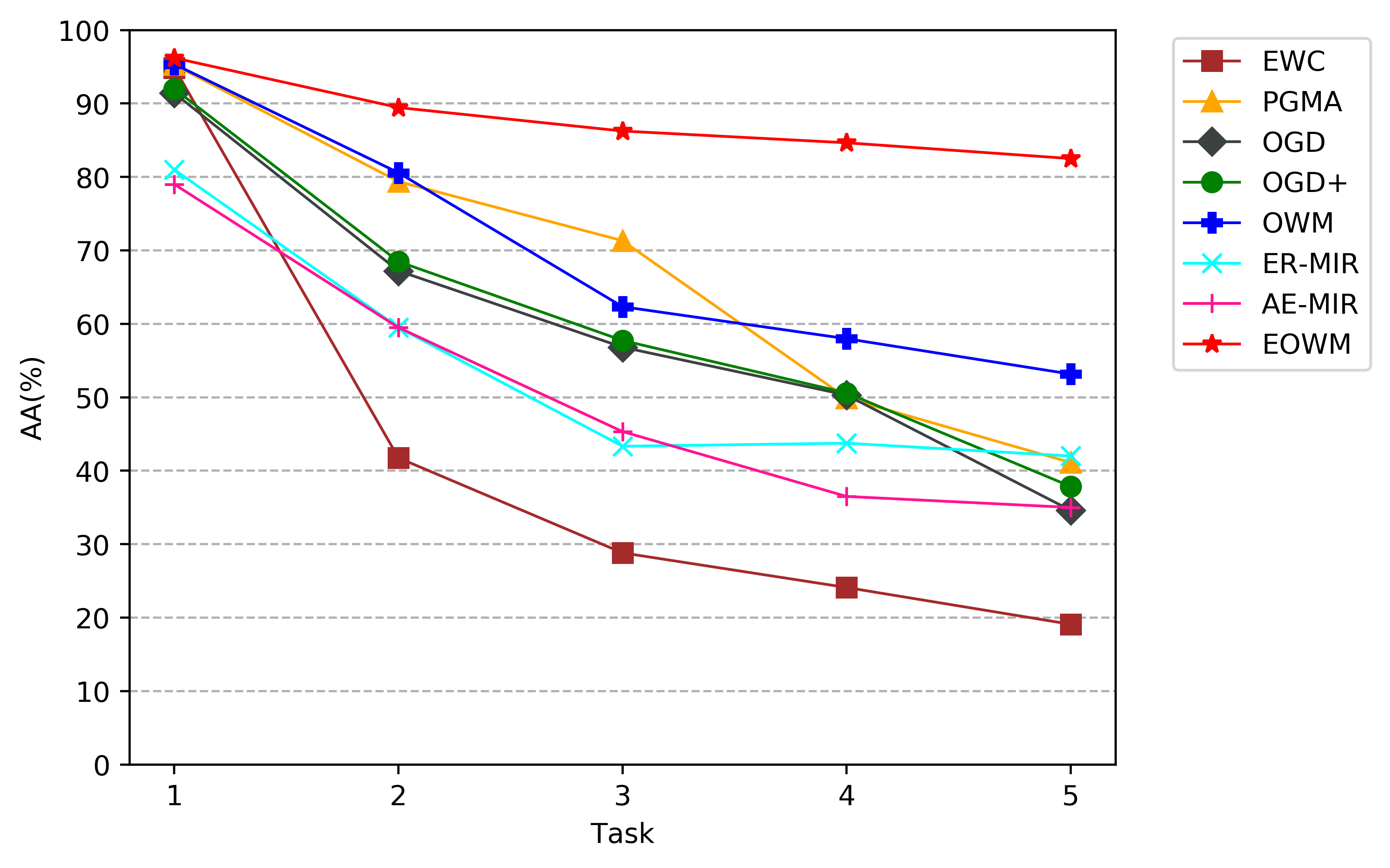
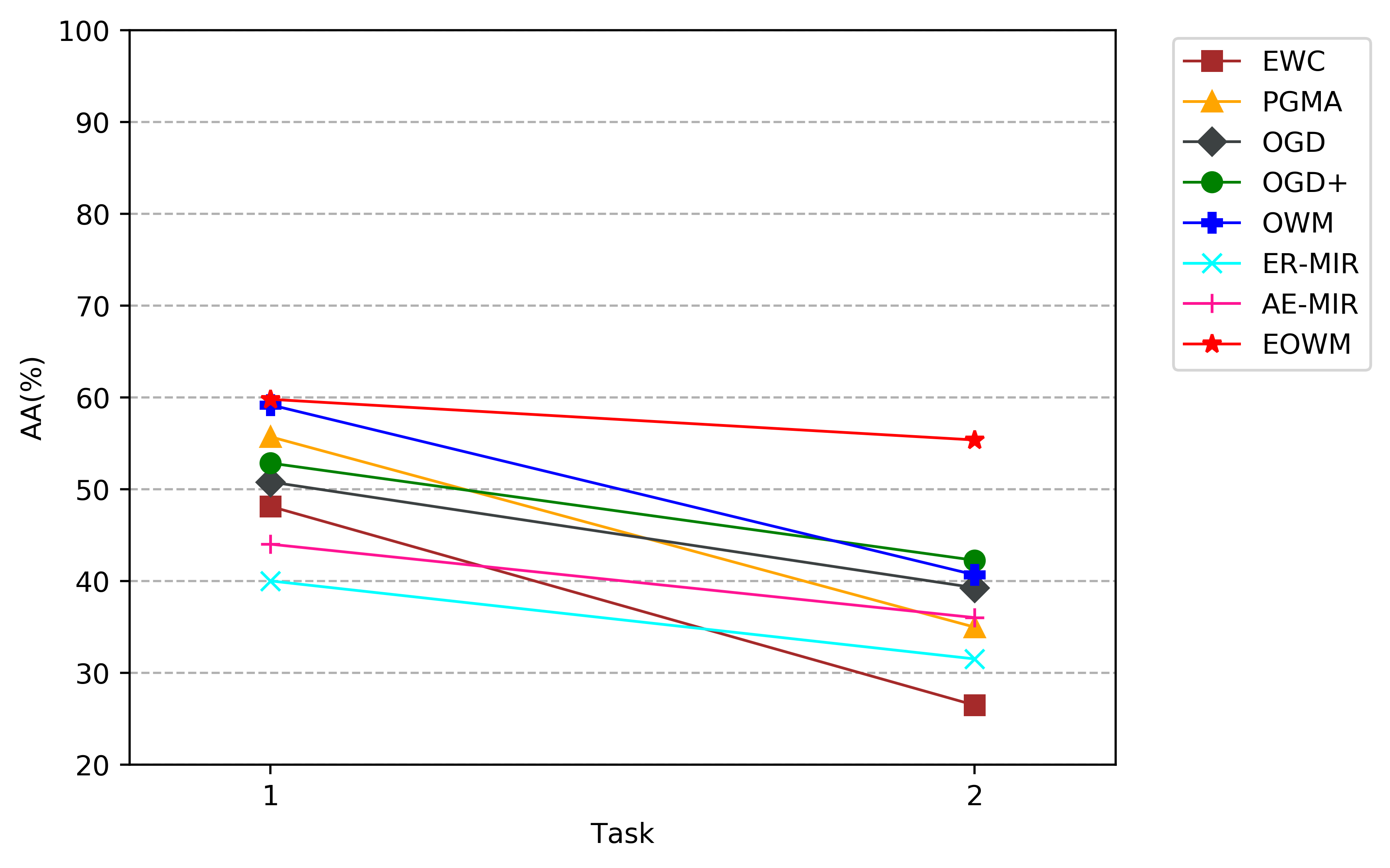
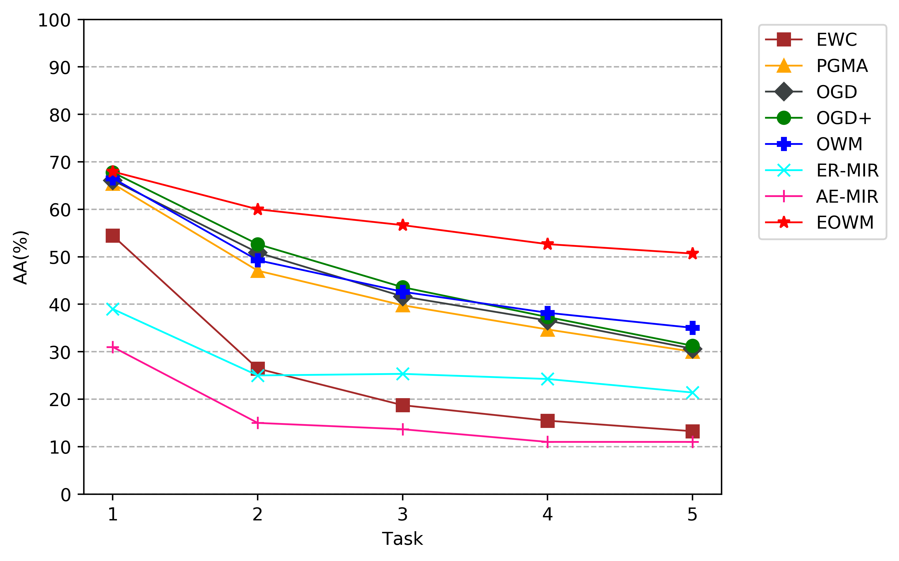
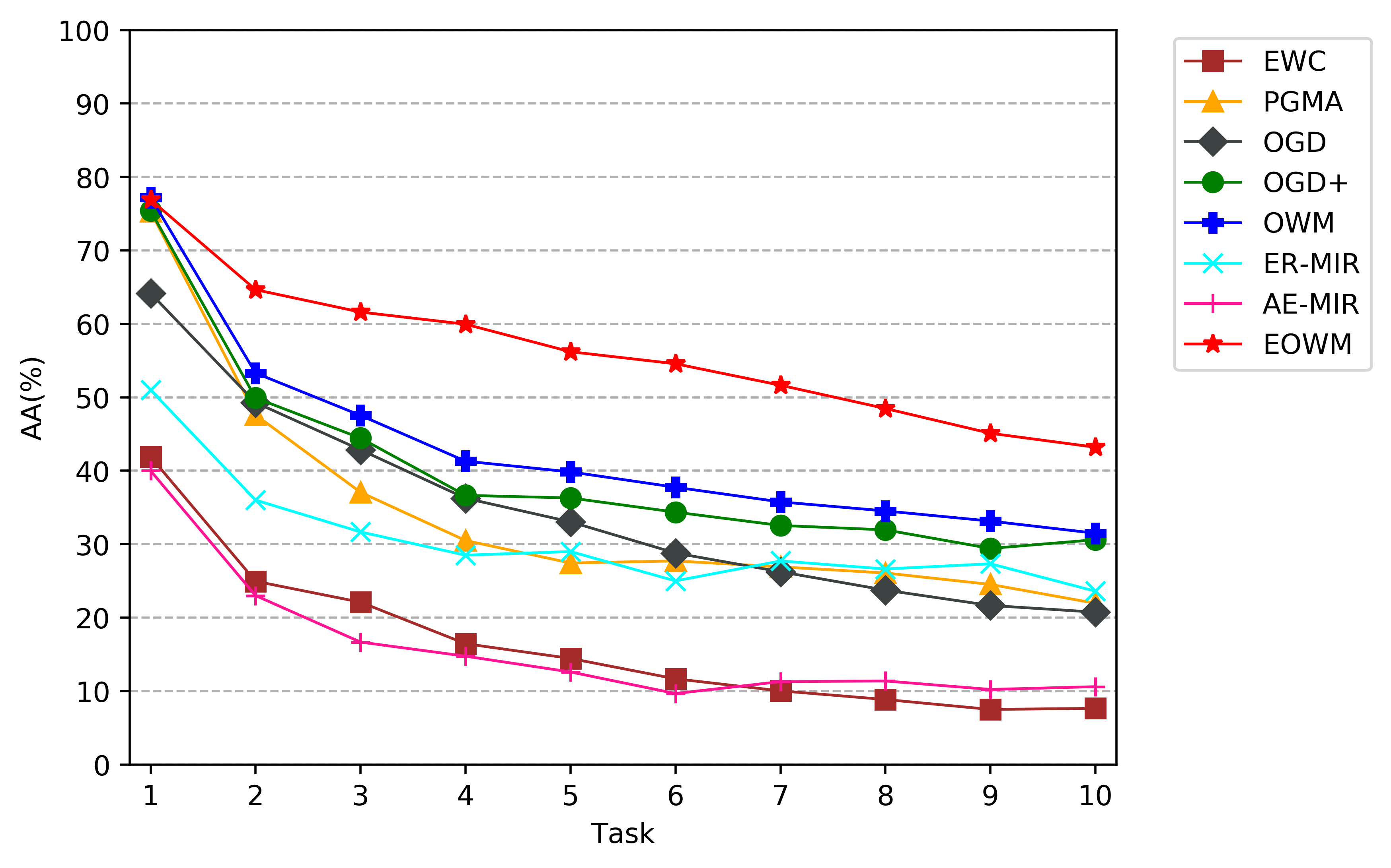
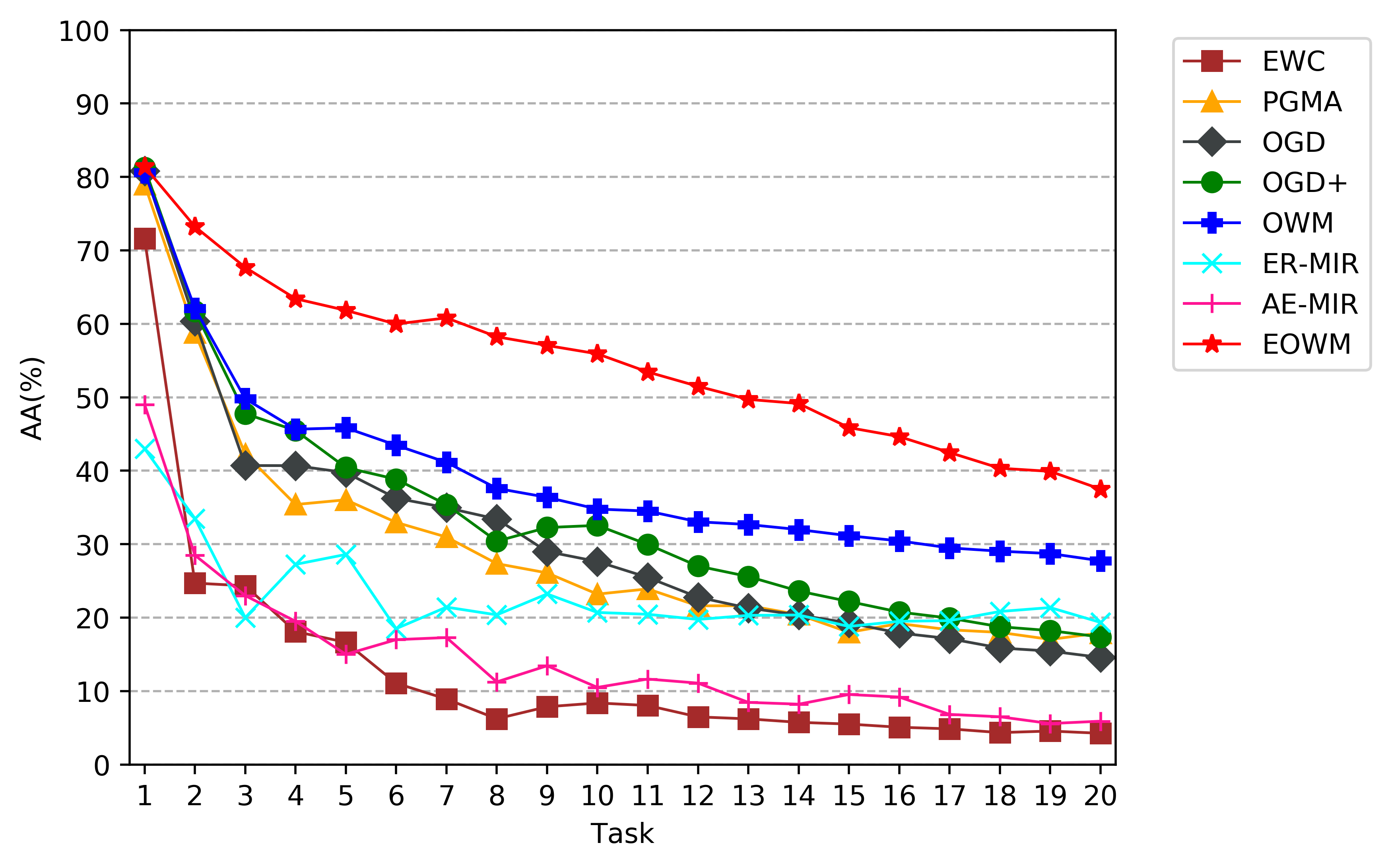
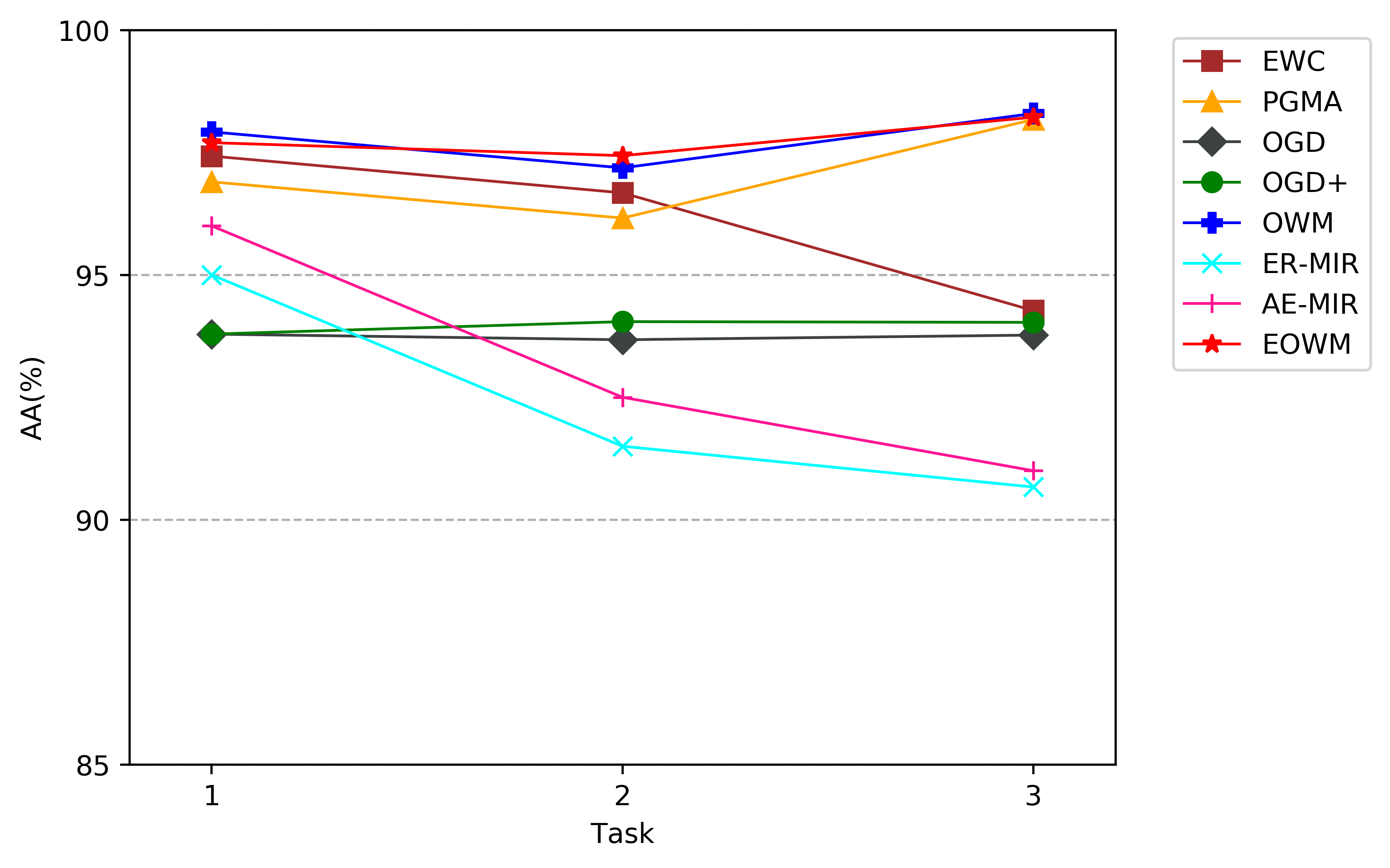
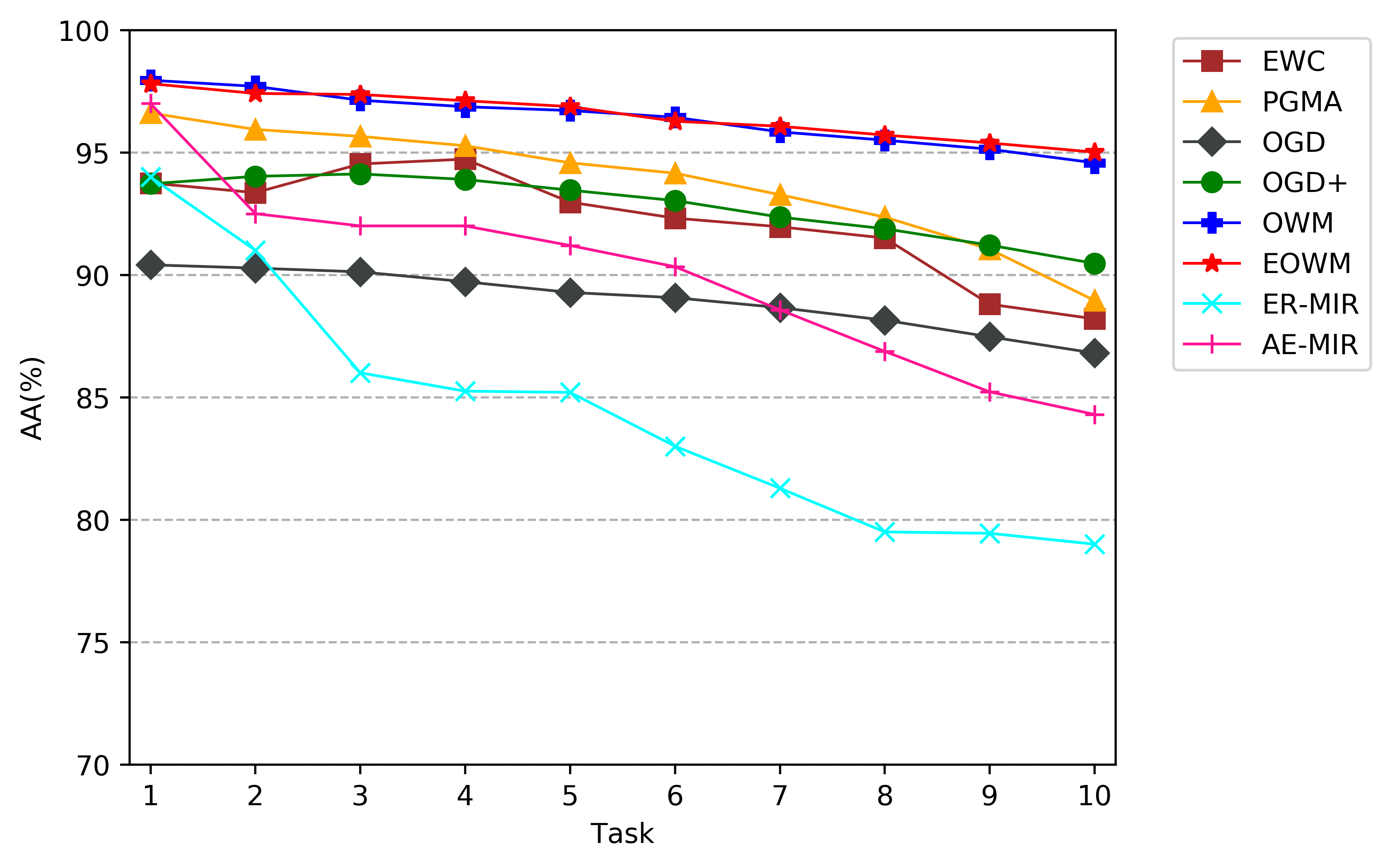
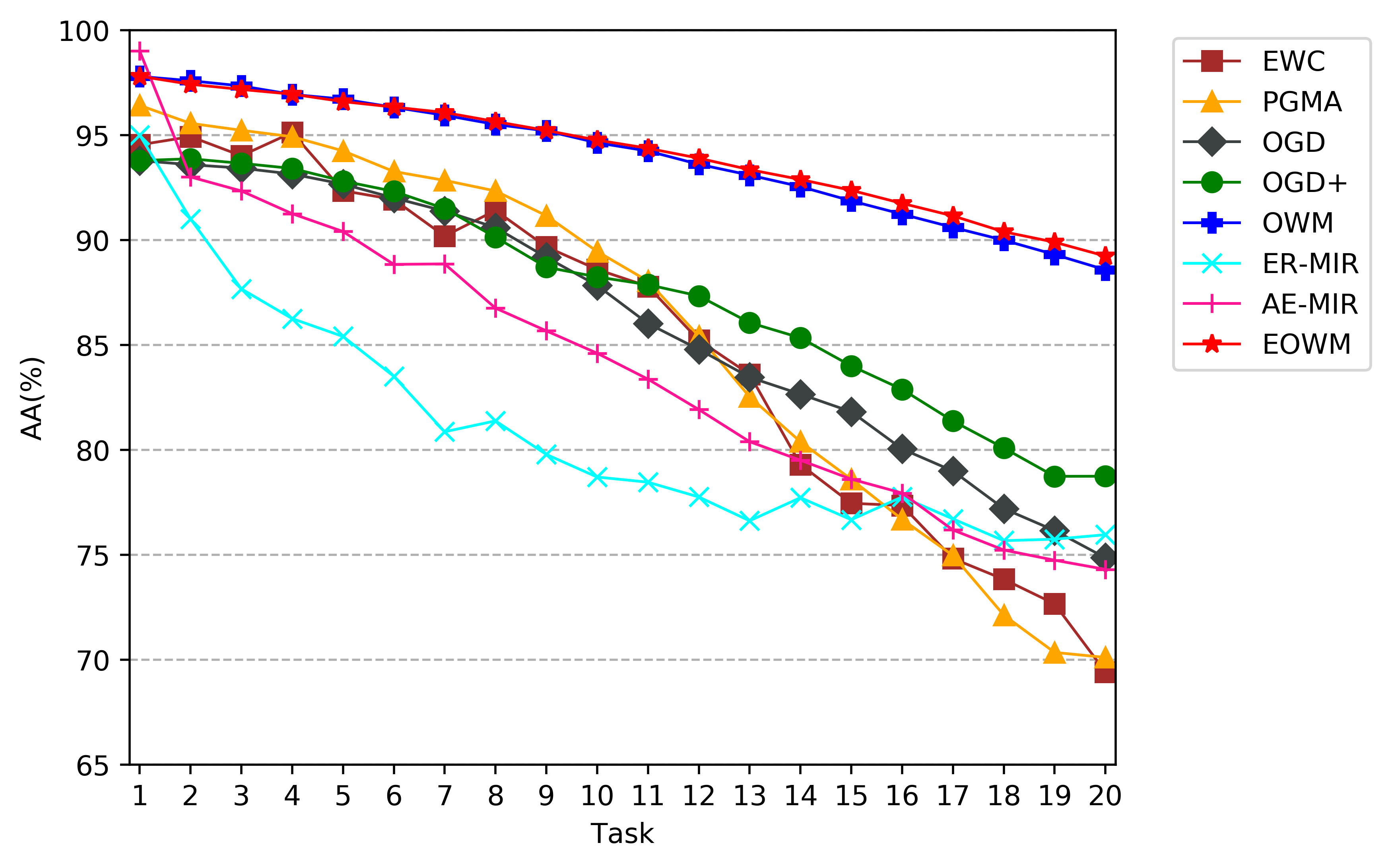
Figure 3: The average accuracy of EOWM and five baselines on Shuffled MNIST, CIFAR-10, and CIFAR-100. (a) CIFAR-10 with 5 tasks, (b) CIFAR-100 with 2 tasks, (c) CIFAR-100 with 5 tasks, (d) CIFAR-100 with 10 tasks, (e) CIFAR-100 with 20 tasks, (f) Shuffled MNIST with 3 tasks, (g) Shuffled MNIST with 10 tasks, (h) Shuffled MNIST with 20 tasks.

In this subsection, we report our evaluation results (the AA and MRR are shown in Table 2 and Fig. 3) of the proposed EOWM and other five baselines in two cases (tasks are similar or dissimilar). From Table 2 and Fig. 3, we can draw the following conclusions.

1) When tasks are similar, the EOWM is consistently superior to other algorithms except in the setting that has three tasks on Shuffled MNIST dataset. In the other three settings on Shuffled MNIST dataset, the difference between the EOWM and the OWM is -0.0002, 0.0058 and 0.0065 with the AA metric, respectively. It indicates that in the case of similar tasks, compared to the OWM, as the number of tasks increases, the EOWM has more advantages in learning the optimal weight of a new task.

2) The EOWM has the highest MRR performance on Shuffled MNIST dataset in the case of similar tasks. The difference between our method and OWM is 0.0015, 0.0041 and 0.0081, respectively. Such a result means that EOWM performs better in alleviating forgetting with the increasing number of tasks when tasks are similar compared to the OWM. Therefore, EOWM has higher potential in finishing continuous learning.

3) When tasks are dissimilar, our EOWM gains the highest accuracy in all settings on CIFAR-10 and CIFAR-100, which means that our EOWM has significant advantages in learning new features of new tasks. Moreover, in the case of dissimilar tasks, our EOWM yields the best MRR, which indicates that properly enlarge the influence of new task does not have a negative impact on alleviating forgetting.

Table 3: The performance of the AA and MRR over 2 tasks under different combinations of $w_{1}$ and $w_{2}$

Metric	Shuffled MNIST(2 Task)
	Coefficient settings	$w_{2}=0.05$	$w_{2}=0.1$	$w_{2}=0.15$
AA	$(w_{1}+w_{2})$=1	97.41	97.45	97.56
MRR		0.9938	0.9964	0.9983
Metric	MNIST(2 Task)
	Coefficient settings	$w_{2}=0.05$	$w_{2}=0.1$	$w_{2}=0.15$
AA	$(w_{1}+w_{2})$=1	87.16	87.43	87.77
MRR		0.7742	0.7780	0.7871

Ablation study:

In this part, we evaluate the effect of the size of the projection of gradient on $\Omega_{n-1}$ and $\Omega_{n-1}^{\perp}$ on the ability of the neural network to learn new knowledge and alleviate forgetting. We fix $w_{1}$ and set $w_{2}$ to different values to adjust the influences of the two gradient projections. We evaluate the impact both using the AA and MRR metrics. When tasks are similar, we shuffle the MNIST and construct two joint tasks, where both have ten classes. However, when tasks are dissimilar, we divide the MNIST dataset into two disjoint tasks, where both have five classes. The neural network consists of two fully connected layers.

As shown in Table 3, when tasks are similar, fixing the value of $w_{1}+w_{2}$, both the AA and MRR of the neural network will increase. The reason is that if we fix $w_{1}+w_{2}$, enlarging $w_{2}$ will decrease $w_{1}$ which means increase the impact of old knowledge and decrease the impact of new knowledge. So the MRR increases and the neural network saves more old knowledge and the AA increases.

When tasks are dissimilar, fixing the value of $w_{1}+w_{2}$, the AA increase and the MRR first rises and then decreases. The reason is that if fixing the value of $w_{1}+w_{2}$, a larger $w_{2}$ indicates a smaller $w_{1}$, which means increase the impact of old knowledge and decrease the impact of new knowledge.As the increase of $w_{2}$, the MRR first rises because of the new knowledge’s influence less than the old knowledge’s and finally decrease because of the new knowledge has great influence when new tasks learning. When the neural network forgets less than it learns, the AA will increase. When the neural network forgets less than it learns, the AA will increase.

Conclusion

In this study, we first theoretically study the essential weaknesses of the existing OWM methods. Then we reveal and prove the facts that: 1) none of the existing $P_{OWM}$ of the OWM methods take advantage of all the necessary knowledge, and 2) the existing methods rely on an unpractical assumption that the classes of sequential tasks are disjoint. We propose a new enhanced projection operator, i.e., $P_{EOWM}$, which takes into account all the knowledge in $P_{OWM}$ and removes the unrealistic assumption. On the bases, we propose a new OWM algorithm EOWM followed by introducing a more reasonable metric. Extensive experiments conducted on the benchmarks demonstrate that our EOWM is superior to all of the state-of-the-art continual learning baselines.

Appendix

A. The proof of Theorem 3

Theorem 3: According to Eq.7, the iterative equation of $P_{EOWM}$ can be obtained as follows.

$$P_{EOWM}^{n+1}=\begin{cases}P_{OWM}^{n+1}(c_{1}I+c_{2}Q^{n+1}),\ T_{prev}\simeq T_{n+1}\\ P_{OWM}^{n+1}(c_{1}I+c_{2}Q_{ort}^{n+1}),\ T_{prev}\not\simeq T_{n+1}\ \end{cases}$$

Proof: The derivation process based on the Recursive Least Square(RLS) method (Shah, Palmieri, and Datum 1992) is as follows. According to Eq.1, the following formula can be obtained.

$$P_{OWM}^{n+1} =I-A_{n}\left(A_{n}^{T}A_{n}+\alpha I\right)^{-1}A_{n}^{T}$$

$$=I-\alpha^{-1}A_{n}\left(\alpha^{-1}A_{n}^{T}A_{n}+I\right)^{-1}A_{n}^{T}$$

Following equation can be obtained by Woodbury Matrix Identity(Gloub and Van Loan 1996).

$$P_{OWM}^{n+1}=(I+\alpha^{-1}A_{n}A_{n}^{T})^{-1}$$

For iterative calculation, the average value $\bar{\textbf{x}}_{j}$ obtained from the data of each task $T_{j}$ is used as the column of the input space, i.e., $A_{n}=(\bar{\textbf{x}}_{1},...,\bar{\textbf{x}}_{n})$.

$$P_{OWM}^{n+1}= (I+\alpha^{-1}A_{n}A_{n}^{T})^{-1}=\alpha(\alpha I+A_{n}A_{n}^{T})^{-1}$$

$$= \alpha(\alpha I+[A_{n-1},\bar{\textbf{x}}_{n}][A_{n-1},\bar{\textbf{x}}_{n}]^{T})^{-1}$$

$$= \alpha(\alpha I+A_{n-1}A_{n-1}^{T}+\bar{\textbf{x}}_{n}\bar{\textbf{x}}_{n}^{T})^{-1}$$

$$= \alpha(\alpha(P_{OWM}^{n})^{-1}+\bar{\textbf{x}}_{n}\bar{\textbf{x}}_{n}^{T})^{-1}$$

Following equation can be obtained by Matrix Inverse Lemma(Gloub and Van Loan 1996) .

$$P_{OWM}^{n+1}= \alpha(\alpha^{-1}P_{OWM}^{n}-\frac{\alpha^{-1}P_{OWM}^{n}\bar{\textbf{x}}_{n}\alpha^{-1}\bar{\textbf{x}}_{n}^{T}P_{OWM}^{n}}{1+\alpha^{-1}\bar{\textbf{x}}_{n}^{T}P_{OWM}^{n}\bar{\textbf{x}}_{n}})$$

Then,

$$P_{OWM}^{n+1}= P_{OWM}^{n}-\frac{P_{OWM}^{n}\bar{\textbf{x}}_{n}}{\alpha+\bar{\textbf{x}}_{n}^{T}P_{OWM}^{n}\bar{\textbf{x}}_{n}}\bar{\textbf{x}}_{n}^{T}P_{OWM}^{n}$$

$$= P_{OWM}^{n}-\boldsymbol{\kappa}_{x}\bar{\textbf{x}}_{n}^{T}P_{OWM}^{n}$$

Similarly, let the average value $\overline{\textbf{W}}_{j}$ obtained from the weights after each task $T_{j}$ trained as the column of the weight space, i.e., $W_{n}=(\overline{\textbf{W}}_{1},...,\overline{\textbf{W}}_{n})$. Then we can directly obtain the iterative formulas of $Q_{ort}$ and $Q$ as follows.

$$\ \ \ \ \ \ \ \ \ \ \ \ \ \ \ \ \ \ \ \ \ \ \ \ \ \ \ \ \ \ \begin{cases}Q_{ort}^{n+1}&=Q_{ort}^{n}-\boldsymbol{\kappa}_{W}\overline{\textbf{W}}_{n}^{T}Q_{ort}^{n}\\ Q^{n+1}&=I-Q_{ort}^{n}\ \ \ \ \ \ \ \ \ \ \ \ \ \ \ \ \ \ \ \ \ \ \ \ \ \ \ \ \ \ \ \ \ \ \ \ \ \hfill\blacksquare\end{cases}$$

B. The proof of Theorem 4

Theorem 4: The time complexity of the EOWM algorithm is $O(N_{c}^{3}N_{n})$, where $N_{c}$ and $N_{n}$ are the number of the columns of the weight and the number of neurons of a layer, respectively(proof shown in Appedix).

Proof: For the learning of any layer $L_{l}$ of neural network, the time complexity of calculating $P_{OWM}$ is $O(N_{c}^{2})$ for each iteration(Shah, Palmieri, and Datum 1992), where $N_{c}$ is the number of columns of the weight of the layer $L_{l}$.

The calculation process of $P_{EOWM}$ shown in Eq.9 includes one matrix addition, one matrix multiplication and two iterations to calculate the projection operator.

According to the process of matrix operation, matrix multiplication has the highest time complexity $O(N_{c}^{3})$. Therefore, the time complexity of calculating $P_{EOWM}$ in each iteration is $O(N_{c}^{3})$.

To sum up, when the network layer $L_{l}$ is trained with the EOWM algorithm, the time complexity is $O(N_{c}^{3}N_{n})$, where $N_{n}$ is the number of neurons of the layer $L_{l}$. $\hfill\blacksquare$

C. The proof of Theorem 5

Theorem 5 : The upper bound of the minimum number of learnable tasks of our proposed EOWM is $rank(P_{EOWM})$, which is fomulated as follows.

$${rank(P_{EOWM})<=\begin{cases}Rank_{OWM}+rank(P_{OWM}Q),\ T_{prev}\simeq T_{n+1}\ \\ Rank_{OWM}+rank(P_{OWM}Q_{ort}),\ T_{prev}\not\simeq T_{n+1}\ \end{cases}}$$

where $Rank_{OWM}$ is the maximum rank of $P_{OWM}$ when $rank(P_{OWM}Q)>0$ and $rank(P_{OWM}Q_{ort})>0$.

Proof: According to Eq.7, when new and old tasks are not similar, the rank of $P_{EOWM}$ can be calculated as follows.

$$rank(P_{EOWM}) =rank(P_{OWM}(c_{1}I+c_{2}Q_{ort}))$$

$$=rank(P_{OWM}+P_{OWM}Q_{ort}))$$

$$<=rank(P_{OWM})+rank(P_{OWM}Q_{ort})$$

According to the analysis of (Zeng et al. 2019), when $\alpha=0$, with the continuous learning of new tasks, the neural network corrected by $P_{OWM}$ will reach its limits, in other words, the rank of $P_{OWM}$ reaches the maximum value recorded as $Rank_{OWM}$, i.e.,

$$rank(P_{OWM})<=Rank_{OWM}$$

From the properties of projection operators, $QQ_{ort}=0$ and $P_{OWM}Q_{ort}\neq 0$, so $rank(P_{OWM}Q_{ort})>0$.

When new and old tasks are similar, the same conclusion can be drawn, which will not be repeated here.$\hfill\blacksquare$

References

- Aljundi et al. (2019) Aljundi, R.; Belilovsky, E.; Tuytelaars, T.; Charlin, L.; Caccia, M.; Lin, M.; and Page-Caccia, L. 2019. Online Continual Learning with Maximal Interfered Retrieval. 11849–11860.
- Amari (1993) Amari, S. 1993. Backpropagation and stochastic gradient descent method. Neurocomputing, 5(4-5): 185–196.
- Bennani and Sugiyama (2020) Bennani, M. A.; and Sugiyama, M. 2020. Generalisation guarantees for continual learning with orthogonal gradient descent. arXiv:2006.11942.
- Caccia et al. (2020) Caccia, M.; Rodríguez, P.; Ostapenko, O.; Normandin, F.; Lin, M.; Page-Caccia, L.; Laradji, I. H.; Rish, I.; Lacoste, A.; Vázquez, D.; and Charlin, L. 2020. Online Fast Adaptation and Knowledge Accumulation (OSAKA): a New Approach to Continual Learning. In Advances in Neural Information Processing Systems 33: Annual Conference on Neural Information Processing Systems 2020, NeurIPS 2020, December 6-12, 2020, virtual, volume 33.
- Chaudhry et al. (2019) Chaudhry, A.; Ranzato, M.; Rohrbach, M.; and Elhoseiny, M. 2019. Efficient Lifelong Learning with A-GEM. In 7th International Conference on Learning Representations, ICLR 2019, New Orleans, LA, USA, May 6-9, 2019. OpenReview.net.
- Chen and Liu (2018) Chen, Z.; and Liu, B. 2018. Lifelong machine learning. Synthesis Lectures on Artificial Intelligence and Machine Learning, 12(3): 1–207.
- Farajtabar et al. (2020) Farajtabar, M.; Azizan, N.; Mott, A.; and Li, A. 2020. Orthogonal gradient descent for continual learning. In The 23rd International Conference on Artificial Intelligence and Statistics, AISTATS 2020, 26-28 August 2020, Online [Palermo, Sicily, Italy], volume 108, 3762–3773. PMLR.
- Gloub and Van Loan (1996) Gloub, G.; and Van Loan, C. 1996. Matrix computations, 3rd. Edition. The Johns Hopkins University, London.
- He and Jaeger (2018) He, X.; and Jaeger, H. 2018. Overcoming catastrophic interference using conceptor-aided backpropagation. In 6th International Conference on Learning Representations, ICLR 2018, Vancouver, BC, Canada, April 30 - May 3, 2018, Conference Track Proceedings. OpenReview.net.
- Hsu, Liu, and Kira (2018) Hsu, Y.; Liu, Y.; and Kira, Z. 2018. Re-evaluating continual learning scenarios: A categorization and case for strong baselines. Computer Research Repository, abs/1810.12488.
- Hu et al. (2019) Hu, W.; Lin, Z.; Liu, B.; Tao, C.; Tao, Z.; Ma, J.; Zhao, D.; and Yan, R. 2019. Overcoming catastrophic forgetting for continual learning via model adaptation. In 7th International Conference on Learning Representations, ICLR 2019, New Orleans, LA, USA, May 6-9, 2019. OpenReview.net.
- Huang et al. (2017) Huang, G.; Liu, Z.; van der Maaten, L.; and Weinberger, K. Q. 2017. Densely connected convolutional networks. In 2017 IEEE Conference on Computer Vision and Pattern Recognition, CVPR 2017, Honolulu, HI, USA, July 21-26, 2017, 2261–2269. IEEE Computer Society.
- Kirkpatrick et al. (2016) Kirkpatrick, J.; Pascanu, R.; Rabinowitz, N. C.; Veness, J.; Desjardins, G.; Rusu, A. A.; Milan, K.; Quan, J.; Ramalho, T.; Grabska-Barwinska, A.; Hassabis, D.; Clopath, C.; Kumaran, D.; and Hadsell, R. 2016. Overcoming catastrophic forgetting in neural networks. arXiv:1612.00796.
- Krizhevsky, Hinton et al. (2009) Krizhevsky, A.; Hinton, G.; et al. 2009. Learning multiple layers of features from tiny images.
- Krizhevsky, Sutskever, and Hinton (2017) Krizhevsky, A.; Sutskever, I.; and Hinton, G. E. 2017. Imagenet classification with deep convolutional neural networks. volume 60, 84–90.
- LeCun, Bengio, and Hinton (2015) LeCun, Y.; Bengio, Y.; and Hinton, G. 2015. Deep learning. nature, 521(7553): 436–444.
- LeCun et al. (1998) LeCun, Y.; Bottou, L.; Bengio, Y.; and Haffner, P. 1998. Gradient-based learning applied to document recognition. Proceedings of the IEEE, 86(11): 2278–2324.
- Lee et al. (2017) Lee, S.; Kim, J.; Jun, J.; Ha, J.; and Zhang, B. 2017. Overcoming Catastrophic Forgetting by Incremental Moment Matching. In Advances in Neural Information Processing Systems 30: Annual Conference on Neural Information Processing Systems 2017, December 4-9, 2017, Long Beach, CA, USA, volume 30, 4652–4662.
- Li et al. (2019) Li, X.; Zhou, Y.; Wu, T.; Socher, R.; and Xiong, C. 2019. Learn to Grow: A Continual Structure Learning Framework for Overcoming Catastrophic Forgetting. In Proceedings of the 36th International Conference on Machine Learning, ICML 2019, 9-15 June 2019, Long Beach, California, USA, volume 97 of Proceedings of Machine Learning Research, 3925–3934. PMLR.
- Li and Hoiem (2016) Li, Z.; and Hoiem, D. 2016. Learning Without Forgetting. In Computer Vision - ECCV 2016 - 14th European Conference, Amsterdam, The Netherlands, October 11-14, 2016, Proceedings, Part IV, volume 9908 of Lecture Notes in Computer Science, 614–629. Springer.
- Lopez-Paz and Ranzato (2017) Lopez-Paz, D.; and Ranzato, M. 2017. Gradient episodic memory for continual learning. In Advances in Neural Information Processing Systems 30: Annual Conference on Neural Information Processing Systems 2017, December 4-9, 2017, Long Beach, CA, USA, 6467–6476.
- McCloskey and Cohen (1989) McCloskey, M.; and Cohen, N. J. 1989. Catastrophic interference in connectionist networks: The sequential learning problem. Elsevier.
- Parisi et al. (2019) Parisi, G. I.; Kemker, R.; Part, J. L.; Kanan, C.; and Wermter, S. 2019. Continual lifelong learning with neural networks: A review. Neural Networks, 113: 54–71.
- Rusu et al. (2016) Rusu, A. A.; Rabinowitz, N. C.; Desjardins, G.; Soyer, H.; Kirkpatrick, J.; Kavukcuoglu, K.; Pascanu, R.; and Hadsell, R. 2016. Progressive neural networks. Computer Research Repository, abs/1606.04671.
- Saad (2003) Saad, Y. 2003. Iterative methods for sparse linear systems. SIAM.
- Shah, Palmieri, and Datum (1992) Shah, S. A.; Palmieri, F.; and Datum, M. 1992. Optimal filtering algorithms for fast learning in feedforward neural networks. Neural Networks, 5(5): 779–787.
- Shen et al. (2020) Shen, G.; Zhang, S.; Chen, X.; and Deng, Z. 2020. Generative Feature Replay with Orthogonal Weight Modification for Continual Learning. arXiv:2005.03490.
- Sinha and Griscik (1971) Sinha, N. K.; and Griscik, M. P. 1971. A stochastic approximation method. IEEE Trans. Syst. Man Cybern., 1(4): 338–344.
- van de Ven and Tolias (2019) van de Ven, G. M.; and Tolias, A. S. 2019. Three scenarios for continual learning. arXiv:1904.07734.
- Wu et al. (2019) Wu, Y.; Chen, Y.; Wang, L.; Ye, Y.; Liu, Z.; Guo, Y.; and Fu, Y. 2019. Large scale incremental learning. In IEEE Conference on Computer Vision and Pattern Recognition, CVPR 2019, Long Beach, CA, USA, June 16-20, 2019, 374–382. Computer Vision Foundation / IEEE.
- Yoon et al. (2018) Yoon, J.; Yang, E.; Lee, J.; and Hwang, S. J. 2018. Lifelong Learning with Dynamically Expandable Networks. In 6th International Conference on Learning Representations, ICLR 2018, Vancouver, BC, Canada, April 30 - May 3, 2018, Conference Track Proceedings. OpenReview.net.
- Zeng et al. (2019) Zeng, G.; Chen, Y.; Cui, B.; and Yu, S. 2019. Continual learning of context-dependent processing in neural networks. Nature Machine Intelligence, 1(8): 364–372.
- Zenke, Poole, and Ganguli (2017) Zenke, F.; Poole, B.; and Ganguli, S. 2017. Continual Learning Through Synaptic Intelligence. In Proceedings of the 34th International Conference on Machine Learning, ICML 2017, Sydney, NSW, Australia, 6-11 August 2017, volume 70 of Proceedings of Machine Learning Research, 3987–3995. PMLR.