Enhanced countering adversarial attacks via input denoising and feature restoring

Abstract

Despite the fact that deep neural networks (DNNs) have achieved prominent performance in various applications, it is well known that DNNs are vulnerable to adversarial examples/samples (AEs) with imperceptible perturbations in clean/original samples. To overcome the weakness of the existing defense methods against adversarial attacks, which damages the information on the original samples, leading to the decrease of the target classifier accuracy, this paper presents an enhanced countering adversarial attack method IDFR (via Input Denoising and Feature Restoring) . The proposed IDFR is made up of an enhanced input denoiser (ID) and a hidden lossy feature restorer (FR) based on the convex hull optimization. Extensive experiments conducted on benchmark datasets show that the proposed IDFR outperforms the various state-of-the-art defense methods, and is highly effective for protecting target models against various adversarial black-box or white-box attacks.

1 INTRODUCTION

In recent years, we have witnessed that deep neural networks (DNNs) have achieved prominent performance in various applications, such as autonomous vehicles, robotics, network security, image/speech recognition, natural language processing, etc. However, a large number of applications and theoretical researches (Amodei et al., 2016; Jia & Liang, 2017; Joshi et al., 2019; Shafahi et al., 2019a; Qi et al., 2021; Zhou et al., 2021) show that the DNNs are vulnerable to adversarial examples/samples (AEs) with imperceptible perturbations in clean/original samples, namely DNNs’ vulnerability against adversarial attacks. Szegedy et al. (2014) proposed the concept of AE, which means that by adding a slight perturbation to the input data, CNNs could easily mis-classify the AEs with high confidence, while human eyes cannot distinguish these subtle differences. The CNNs’ vulnerability raises both theory-wise issues about the interpret-ability of deep learning and application-wise issues when deploying the CNNs in security-sensitive applications (Shi et al., 2021).

To overcome the above issues, many methods of defending the AEs have been proposed, which can roughly fall into the following three categories. The first category is to enhance the robustness of CNNs itself. Adversarial training methods (Shafahi et al., 2019b; Tramèr et al., 2020; Ding et al., 2020; Wang et al., 2020; Zheng et al., 2020; Wong et al., 2020; Pang et al., 2020; Stutz et al., 2020; Gokhale et al., 2021) are the representatives among them. These methods inject AEs into the training data to retrain the CNNs. Label smoothing methods, e.g., methods (Warde-Farley & Goodfellow, 2016; Papernot et al., 2016b) convert one-hot labels to soft targets, also belonging to this class. Another one refers to the various pre-processing/purification methods (Gu & Rigazio, 2015; Guo et al., 2018; Song et al., 2018; Jia et al., 2019; Yoon et al., 2021), which focus on shifting the AEs back to their clean data representations, namely purification. It’s worth noting that the self-supervised learning methods (Mao et al., 2019; Hendrycks et al., 2019; Naseer et al., 2020; Chen et al., 2020b; Shi et al., 2021) have emerged recently and formed the third category. Studies have shown that the self-supervised learning can improve adversarial robustness more recently. These methods generally combine self-supervised learning with adversarial training to achieve the adversarial purification.

Although many adversarial defense methods have achieved their competitive robustness performance , we have observed the fact that all of the existing methods suffer from a key weakness, i.e., they focus on defending against adversarial attacks, but ignore the information loss/the partial knowledge forgetting learned by the CNN model for clean samples during the adversarial training/purification process, which leads to a decrease in the target classifier accuracy, which is a serious secondary disaster caused by the adversarial attacks to CNNs robustness. We suggest that an effective adversarial defense method must address this issue. To bridge the gap and to overcome the weakness, this paper presents a novel and enhanced countering adversarial attack method IDFR (via Input Denoising and Feature Restoring). The proposed IDFR consists of an input denoiser (ID) and a hidden lossy feature restorer (FR). The ID is used for enhanced denoising/pre-processing input AEs, and the FR is used for restoring the hidden lossy features of the clean samples based on the convex hull optimization.

Compared with the above three types of the state-of-the-art representative adversarial defense methods, e.g., the methods (Liao et al., 2018; Guo et al., 2018; Xu et al., 2018; Jia et al., 2019; Naseer et al., 2020; Wong et al., 2020; Shi et al., 2021), etc., our proposed IDFR has the following distinct advantages. First, based on a new designed ID with a U-Net convolutional network (Ronneberger et al., 2015), and with the joint training of AEs and enhanced clean samples, i.e., clean samples with Gaussian disturbance augmentation, our IDFR achieves stronger input denoising capability, and its ID can effectively prevent over-fitting to AEs. Second, with the convex hull optimization (Boyd et al., 2004), the linear convex combinations of the hidden features of the denoising AEs and clean samples with misclassification are devised to train the FR of the IDFR, leading to effectively recovering the lossy information on the clean samples and avoiding the decrease of the target classifier accuracy. Third, both the components ID and FR in the IDFR are pluggable, and they can be transferred across different target models. Extensive experiments conducted on benchmark datasets show that the performance of our proposed method IDFR greatly outperforms that of the state-of-the-art defense methods, and is consistently effective in protecting target classifiers against AEs and lossy clean samples.

2 Preliminary and related work

2.1 Preliminary

Adversarial examples AEs Biggio et al. (2013) found adversarial attack phenomenon, and Szegedy et al. (2014) proposed AEs to fool DNNs. Adding a subtle perturbation to the input of a DNN will produce an error output with high confidence, while human eyes cannot recognize the difference. Suppose that there are a target model $f_{\theta}$ and an original/clean example $x$, which can be correctly classified by the model, i.e., $f_{\theta}(x)=y$, where $y$ is the true class label of $x$. However, it is possible to construct an AE $x^{\prime}$ which is perceptually indistinguishable from $x$ but is classified incorrectly, i.e., $f_{\theta}(x^{\prime})\neq y$.

Problem statement Consider an encoder $f_{enc}$: $h_{x}=f_{enc}(x;\theta_{enc})$, a classifier $f_{cls}(h_{x};\theta_{cls})$ on top of the representation/embedding $h_{x}$, and the target model $f=f_{cls}\circ f_{enc}$, a composition of the encoder and the classifier. The adversarial denoising/purification problem can be formulated as follows: for an adversarial example $x^{\prime}$ and its clean counterpart $x$, our denoising/purification strategies $\pi_{1}$ and $\pi_{2}$ aim to: 1) find $x^{*}=\pi_{1}(x^{\prime})$ that is as close to the clean/original example $x$ as possible: $x^{*}\rightarrow x$, and 2) achieve $y_{h_{x}}=\pi_{2}(y_{h_{\tilde{x}}}$), i.e., $y_{h_{\tilde{x}}}\rightarrow y_{h_{x}}(=y)$, where $\tilde{x}$ is the lossy example corresponding to a clean example $x$ partially damaged by the previous denoising operation, $h_{\tilde{x}}=f_{enc}(\tilde{x})$, and $y_{h_{\tilde{x}}}=f_{cls}(h_{\tilde{x}})$. However, this problem is under-determined as different clean examples can share the same adversarial counterpart, i.e., there might be multiple or even infinite solutions for $x$. Thus, we consider the following relaxation

$$\min_{\pi_{1}}\mathcal{L}_{cls}\bigl{(}f_{cls}(x^{*}),y\bigr{)}+\min_{\pi_{2}}\mathcal{L}_{cls}\bigl{(}f_{cls}(h_{\tilde{x}}),y\bigr{)}$$ (1)

$$\text{s.t.}\quad\|x^{*}-x^{\prime}\|\leq\epsilon,\;\;x^{*}=\pi_{1}(x^{\prime}),\;\;y_{h_{x}}=\pi_{2}(y_{h_{\tilde{x}}})=y$$

where $\mathcal{L}_{cls}$ is the cross entropy loss for the classifier and $\epsilon$ is the budget of adversarial perturbation.

It is worth noting that, to our knowledge, this is the first time we presented the complete formal definition of the problem. In addition, the existing adversarial defense methods only achieve the above adversarial defense strategy $\pi_{1}$ well, but ignore/do not achieve the $\pi_{2}$.

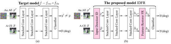
Figure 1: The schematic diagram of the target model (a) and the proposed model IDFR (b).

2.2 Related work

In recent years, for the severe challenge of adversarial attacks to CNNs, many adversarial defense methods have been proposed, which can be roughly divided into the following three categories. As space does not allow for a comprehensive literature study, we refer readers to Shafahi et al. (2019a); Yuan et al. (2019); Zhang & Li (2020); Chen et al. (2020a); Machado et al. (2020) for a survey of these works. Hereby, we only focus on some latest state-of-the-art methods relevant to our study.

Adversarial training Adversarial training aims to improve CNNs’ robustness through data augmentation, where the target model is trained on adversarial perturbed examples, i.e., AEs, instead of clean/original training samples (Shafahi et al., 2019b; Ding et al., 2020; Wang et al., 2020; Pang et al., 2020; Stutz et al., 2020; Gokhale et al., 2021). By solving a min-max problem, the model learns a smoother data manifold and decision boundary, which improves robustness of the DNNs. However, the computational costs of the general adversarial training methods are high as strong adversarial examples are typically found in an iterative manner with heavy gradient calculation. To overcome the weakness, Wong et al. (2020) revealed that adversarial training with the fast gradient sign method FGSM (Goodfellow et al., 2015), when combined with random initialization, is as effective as PGD-based training (Madry et al., 2018) but has a significantly lower cost.

Adversarial denoising/purification This kind of robust learning focuses on shifting the AEs back to the clean counterparts, namely adversarial denoising/purification. Representative methods are DCN (Gu & Rigazio, 2015), HGD (Liao et al., 2018), Defense-GAN (Samangouei et al., 2018), ComDefend (Jia et al., 2019), NPR (Naseer et al., 2020), Feature Squeezing (Xu et al., 2018), JPEG Compression & TVM (Guo et al., 2018), ADP (Yoon et al., 2021), etc. Gu & Rigazio (2015) exploited a general DAE (Vincent et al., 2008) to remove adversarial noises. Samangouei et al. (2018) trained a GAN on clean examples and projected the AEs to the manifold of the generator, but the GAN was hard and inefficient to train. Jia et al. (2019) proposed an end-to-end image compression model ComDefend to defend against AEs, and defeated the state-of-the-art defense models including the winner (Liao et al., 2018) of NIPS 2017 adversarial challenge. Guo et al. (2018) introduced two defense models, i.e., JPEG Compression & TVM, with their best defense eliminating 60% of strong gray-box and 90% of strong black-box attacks by their defense methods. Yoon et al. (2021) proposed a novel adversarial purification method ADP based on an energy-based model trained with denoising score-matching, and the proposed ADP could quickly purify attacked images within a few steps.

Self-supervised learning Self-supervised learning aims to learn intermediate representations of unlabeled data that are useful for unknown downstream tasks. More recently, studies have shown how self-supervised learning can improve adversarial robustness, leading to the new type of self-supervised learning methods. Mao et al. (2019) discovered that adversarial attacks fool the networks by shifting latent representation to a false class. Hendrycks et al. (2019) observed that PGD adversarial training along with an auxiliary rotation prediction task improved robustness. Naseer et al. (2020) utilized feature distortion as a self-supervised signal to find transferable attacks that are generalized across different architectures and tasks. These methods typically combine self-supervised learning with adversarial training, and thus the computational cost is still high. In contrast, with a variety of self-supervise signals as auxiliary objectives, SOAP (Shi et al., 2021) achieved a competitive robust accuracy by test-time purification, but its test-time computation and accuracy still leaved rooms for improvement.

Although the above various adversarial defense methods have achieved a competitive robust accuracy, we observe the fact that these methods suffer from a serious weakness, i.e., they focus mainly on defending against AEs attacks, but ignore the information loss/the partial knowledge forgetting learned by the CNNs model of the clean samples during the adversarial training/purification process, which leads to a decrease in the target classifier accuracy. In this paper, we aim to bridge the gap and to overcome the key weakness. Specifically, we try to obtain the optimal solution of the problem against adversarial attacks (see Subsec 2.2 problem statement).

3 Input denoising and feature restoring method: IDFR

3.1 Overview of the proposed IDFR

To eliminate the key weakness of existing methods, we propose a novel adversarial defense method IDFR, which consists of two independent but collaborative models, i.e., the input denoiser (ID) and the hidden lossy feature restorer (FR). The structure of the IDFR is shown in Fig. 1.

More specifically, the ID can transform an adversarial image to its clean version, which is a pre-processing module and does not modify the target model structure during the whole process, while the FR is used to restore those partially damaged clean samples {$\tilde{x}$} so that they can be correctly classified under the constrain of the invariance of the denoised samples {$x^{*}$} produced by the ID. For efficiently recovering these {$\tilde{x}$}, the input of the FR takes the embedding of the $\tilde{x}$ generated by the target model encoder $f_{enc}$ rather than $x$ itself. The reason is that the dimension of the embedding is much smaller than that of $x$. Therefore, our FR module is designed as a pluggable component after the output of the target model encoder $f_{enc}$. Ultimately, both the ID and FR of our IDFR jointly enhance/protect the classifier’s robustness of the target model. The design ideas and the theoretical basis behind our proposed IDFR will be detailed in following subsections.

3.2 Input denoiser ID

Network architecture of the ID Although DAE (Denoising AutoEncoder) (Tramèr et al., 2020) is a popular denoising model, it has a bottleneck structure between the encoder and decoder. This bottleneck may constrain the transmission of fine-scale information necessary for reconstructing high-resolution images. We introduce the U-Net convolutional network (Ronneberger et al., 2015) as the network model of our ID. It is due to the fact that the U-Net network can overcome the bottleneck of the DAE. the U-Net network has both a contracting path to extract contextual information and a symmetric expanding path to capture precise local information. Our ID network architecture is shown in Appendix A.1.

Training of the ID Let the ID model be $I_{w}(\cdot)$ with the input an AE $x^{\prime}$ and/or a clean example (CE) $x$, where $w$ is the parameters of the ID. We expect that the output of the ID is the denoised sample $x^{*}$ of $x$. Thus, the optimal objective of the ID is designed as follows

$$\mathcal{L}_{\text{ID}}=\arg\max_{w}\sum\mathbb{I}\Bigl{(}f_{cls}\bigl{(}I_{w}(x,x^{\prime})\bigr{)}=y\Bigr{)}$$ (2)

where $f_{cls}$ is the classifier of the target model $f$, $y$ is the ground truth class label of both $x$ and $x^{\prime}$, and $\mathbb{I}(\cdot)$ is an indicating function. $\mathbb{I}(true)=1$, otherwise $\mathbb{I}(false)=0$. As the $\mathbb{I}(\cdot)$ would result in the issue of gradient disappearances with the back propagation optimization, we replace it with the cross entropy loss, leading to the following Eq. 2

$$\mathcal{L}_{\text{ID}}=\arg\min_{w}\Bigl{(}-\sum y\log f_{cls}\bigl{(}I_{w}(x,x^{\prime})\bigr{)}=y\Bigr{)}$$ (3)

It’s worth noting that our ID adopts the jointly training with both AEs and clean examples to avoid its over-fitting the AEs. Moreover, when the adversarial disturbance of the AE is large, i.e., the adversarial attack is strong, the ID’s learning will favor this strong AE, i.e., the ID would over-fitting the strong AE. To address the issue, the multi-round Gaussian perturbation data enhancement method (Jeong & Shin, 2020) is employed to obtain the enhanced counterpart $x_{e}$ of $x$, which greatly improves the ID model’s learning to clean samples $x$. Therefore, considering the above two factors, the ID model adopts the joint training with such training datasets including both {$x^{\prime}$} and {$x_{e}$}. By being equipped with the U-Net network and the enhanced jointly training strategy, our ID achieves a stronger ability of the adversarial denoising and model generalization than that of the existing denoising/purification strategies. The ID training algorithm is shown in Algorithm 1.

3.3 Lossy features restorer FR

3.3.1 The design motivation of the FR

As the above discussion, we have known that there may be residual noises/information damaged in the generated outputs $x^{*}$/$x$ (denoted as $\tilde{x}$) when $x$ and $x^{\prime}$ are fed into the ID, and that the effect of the residual noises/information damaged in the $x^{*}$/$\tilde{x}$ increase rapidly along with the depth of the target model. Note that this is the infrasonic disaster caused by adversarial attacks, which also poses a great threat to the robustness of the target model. Therefore, it is essential that such disaster/threat should be dealt with effectively. To this end, the network structure and learning/training process of the FR should be well-designed. Similar to the ID network, the FR network also utilizes the U-Net network, whose structure and hyperparameters are shown in Appendix A.1.

3.3.2 Training of the FR

By the theoretical study and extensive experiments, we have found that some of these outputs {$x^{*}$} and {$\tilde{x}$} of the ID can be correctly classified by the target model’s classifier $f_{cls}$, while a few others get mis-classified. As we pointed out earlier, this phenomenon is an infrasonic disaster caused by adversarial attacks that must be contained and resolved well. From this point of view, we devised a novel learning/ training strategy of the FR. For the efficiency of our FR learning/training, we only consider the embeddings $h_{x^{*}}$ and $h_{x}$/$h_{\tilde{x}}$ generated by the target model encoder, i.e., $h_{x^{*}}=f_{enc}(x^{*}),h_{x}=f_{enc}(x)$, and $h_{\tilde{x}}=f_{enc}(\tilde{x})$ as the input of our FR, which is due to the fact that the dimension of the embedding is much smaller than that of a raw data itself. For clarifying our proposed FR’s learning/training algorithm, following definitions and Theorem 1 are first introduced.

Definition 1: Classified space of data. For a specific category of input data, we define $p_{1}$ as the space where the embeddings, i.e., $h_{x^{*}}$ and $h_{x}$/$h_{\tilde{x}}$, can be correctly classified by the target classifier $f_{cls}$, and $p_{2}$ as the space where embeddings are misclassified. The complete classification space of the embeddings is defined as $p$, i.e., $p=p_{1}\cup p_{2}$. To simplify the notation, those embeddings falling into $p_{1}$ are uniformly denoted as $\hat{\textbf{x}}=\{h_{x}\}$, while the others falling into $p_{2}$ are represented by $\hat{\textbf{x}}^{\prime}=\{h_{\tilde{x}}\}$. The schematic diagram of the classified spaces and the convex hull is shown Fig. 3.

Definition 2: Convex hull $Co(\cdot)$. For a given data set $\textbf{x}\in\mathbb{R}$, the intersection of all convex sets containing the x is called the convex hull of x, denoted as $Co(\textbf{x})$, which can be constructed from a convex combination of all points in x (Boyd et al., 2004).

Based on the theory of convex hull optimization (Boyd et al., 2004), the following Theorem 1 can be introduced and proved (see Appendix A.2).

Theorem 1.

A convex combination of any two points in a $Co(\cdot)$ remains in the $Co(\cdot)$ region.

According to the above definitions and Theorem 1, we can obtain the convex hull $Co(\hat{\textbf{x}}\cup\hat{\textbf{x}}^{\prime})$ of both $\hat{\textbf{x}}=\{h_{x}\}$ and $\hat{\textbf{x}}^{\prime}=\{h_{\tilde{x}}\}$ as follows

$$Co(\hat{\textbf{x}}\cup\hat{\textbf{x}}^{\prime})=\{\alpha h_{x}+(1-\alpha)h_{\tilde{x}}|h_{x}\in\hat{\textbf{x}},h_{\tilde{x}}\in\hat{\textbf{x}}^{\prime}\}$$ (4)

where $\alpha$ is an equilibrium coefficient between 0 and 1. That is, the smaller the value of $\alpha$, the closer to $h_{\tilde{x}}$ the convex hull $Co(\hat{\textbf{x}}\cup\hat{\textbf{x}}^{\prime})$ is, and vice versa.

How can we use the FR to restore the clean sample with damaged information and the AE with residual noise, i.e., $\hat{\textbf{x}}^{\prime}=\{h_{\tilde{x}}\}$, so that they can finally be correctly classified? This question is essentially equivalent to this: How can we pull the $\hat{\textbf{x}}^{\prime}=\{h_{\tilde{x}}\}$ from the misclassified region $p_{2}$ back into the correctly classified region $p_{1}$ by the FR? To this end, based on the convex hull optimization (Boyd et al., 2004), and inspired by the method mixup (Zhang et al., 2018), i.e., a data augmentation method, we devised the following optimal learning/training strategy for our FR model, denoted as $F_{\pi}(\cdot)$, where $\pi$ represents the parameters of the FR model. Specifically, 1) to pull the $\hat{\textbf{x}}^{\prime}=\{h_{\tilde{x}}\}$ from the misclassified region $p_{2}$ back into the correctly classified region $p_{1}$, and 2) to maintain those correctly classified data $\hat{\textbf{x}}=\{h_{x}\}$ still in its classified area $p_{1}$, we proposed the cross entropy loss of the FR as follows.

$$\mathcal{L}_{FR}=\arg\min_{\pi}\bigl{(}-\sum y\log f_{cls}\bigl{(}F_{\pi}(h_{\tilde{x}})\bigr{)}-\sum y\log f_{cls}\bigl{(}F_{\pi}(h_{x})\bigr{)}\bigr{)}$$ (5)

where the first part in Eq. 5 is used to accomplish the first objective above, and the second part is used to achieve the second objective. It is worth mentioning that in order to achieve its end and to improve the generalization ability of the FR model, the Eq. 5 is not directly used in the training process of our FR model, but another form Eq. 6 is utilized.

Since the data $\hat{\textbf{x}}=\{h_{x}\}$ and/or $\hat{\textbf{x}}^{\prime}=\{h_{\tilde{x}}\}$ in the regions $p_{1}$ and $p_{2}$, respectively, are all in the $Co(\hat{\textbf{x}}\cup\hat{\textbf{x}}^{\prime})$, based on the convex hull optimization theory (Boyd et al., 2004), the Eq. 5 can be converted into Eq. 6.

$$\mathcal{L}_{FR}=\arg\min_{\pi}\bigl{(}-\sum y\log f_{cls}\bigl{(}F_{\pi}(\alpha h_{x}+(1-\alpha)h_{\tilde{x}}\bigr{)}\bigr{)},h_{x},h_{\tilde{x}}\in Co(\hat{\textbf{x}}\cup\hat{\textbf{x}}^{\prime}),\alpha\in[0,1]$$ (6)

Equipped with the loss function $\mathcal{L}_{FR}$ and the convex hull $Co(\hat{\textbf{x}}\cup\hat{\textbf{x}}^{\prime})$, the FR can achieve its end well. The training process of the proposed FR is shown in Algorithm 2.

From the above discussion, it can be clearly seen that, different from all the existing adversarial defense methods, with the ID and FR, our proposed method IDFR solves the problem (see Eq. 1) of the defense against adversarial attacks well, which is also fully verified by our extensive experimental results.

Algorithm 1 The training process of ID

1:Target model $f_{\theta}(\cdot)$, produce the $\epsilon$ model $A(\cdot)$, ID model $I_{w}(\cdot)$, training epochs $T$, training datasets $\{x\}$ and $\textbf{x}_{e}$, learning rate $\lambda$

2:ID model $I_{w}$

3:for each $x$ in {$x$} do

4:     $x^{\prime}\leftarrow x+\epsilon,y^{\prime}\leftarrow y$

5:     $\textbf{x}^{\prime}\leftarrow\textbf{x}^{\prime}\cup\{(x^{\prime},y^{\prime})\}$

6:end for

7:for each $i\in 1,\cdots,T$ do

8:     for each $(x^{\prime},y)$ in $\textbf{x}^{\prime}\cup\textbf{x}_{e}$ do

9:         Update $w$ by Eq. 3 with Adam

10:     end for

11:end for

12:return $I_{w}$

Algorithm 2 The training process of FR

1:Target model $f_{\theta}(\cdot)$, pretrained ID model $I_{w}(\cdot)$, FR model $F_{\pi}(\cdot)$, Training epochs $T$, enhenced samples $\textbf{x}_{e}$, learning rate $\eta$

2:FR model $F_{\pi}(\cdot)$

3:for each $i=1$ to $T$  do

4:     for $h_{x},h_{\tilde{x}}$ in $Co(\hat{\textbf{x}}\cup\hat{\textbf{x}}^{\prime})$  do

5:         $\alpha\leftarrow\text{rand}(0,1)$

6:         Calculate $\alpha h_{x}$

7:         Calculate $(1-\alpha)h_{\tilde{x}}$

8:         Calculate $Co(\cdot)=\alpha h_{x}+(1-\alpha)h_{\tilde{x}}$

9:         Update $\pi$ by Eq. 6 with Adam

10:     end for

11:end for

12:return $F_{\pi}$

4 Experiments

In this study, all experiments were conducted on the server: Intel Xeon(R) Gold 5115 CPU @ 2.40GHz, 97GB RAM and NVIDIA Tesla P40 graphics processor.

4.1 Target models, baselines, datasets and experimental settings

Target models and baselines To fully evaluate the performance of our proposed IDFR, in this paper, the following various typical CNN models, i.e., VGG16 (Liu & Deng, 2015), ResNet18 (He et al., 2016), InceptionV3 (Szegedy et al., 2016) and ResNet50 (He et al., 2016), are employed as the target models, seven methods belong to the three different types of the state-of-the-art adversarial defense methods, i.e., ComDefend (Jia et al., 2019), NPR (Naseer et al., 2020), Feature Squeezing (Xu et al., 2018), JPEG Compression & TVM (Guo et al., 2018), ADP (Yoon et al., 2021), Fast AT(Goodfellow et al., 2015) and SOAP (Shi et al., 2021) are used as experimental baselines, where the ComDefend, Feature Squeezing, JPEG Compression & TVM and ADP belong to the category of the adversarial denoising/purification, both NRP and SOAP improve adversarial robustness of the target models by self-supervised learning, while the method Fast AT falls into the class of the adversarial training.

Datasets 1) MNIST (LeCun et al., 1998): this dataset consists of 70,000 28$\times$28 black-and-white images of handwritten digits from 0 to 9. We use 60,000/3000/7000 images for training/validation/testing respectively. 2) CIFAR-10 (Krizhevsky et al., 2009): this dataset consists of 60,000 32$\times$32 color images of 10 classes, with 6000 images per class. We use 50,000/3000/7000 images for training/validation/testing respectively. 3) CIFAR-100 (Krizhevsky et al., 2009): this dataset consists of 60,000 32$\times$32 color images of 100 classes, with 600 images per class. We use 50,000/3000/7000 images for training/validation/testing respectively. 4) ImageNet (Deng et al., 2009): this dataset consists of 30,000 224$\times$224 color images of 1000 classes, with 30 images per class. We use 25,000/5000/10,000 images for training/validation/testing respectively. 5) SVNH (Netzer et al., 2011): this dataset consists of 624,420 32$\times$32 color images, where 73,257/531,131/26,032 samples are used for training/extra training/testing, respectively. The extra training samples mean they are somewhat less difficult samples to use as extra training data.

Hyperparameter Settings: The training epochs for our ID and FR models are set 100 and 80, respectively, and the learning rates of the models ID and FR are uniformly set to 0.01 for updating the models’ parameters by the adam optimizer. For all the baselines’ hyperparameter settings, we strictly follow the settings of the original papers.

4.2 Experimental results

4.2.1 Attacking models

The model used to generate adversarial attacks is called the attacking model, which can be a single model or an ensemble of models (Tramèr et al., 2020). When the attacking model is the target model itself or contains the target model, the resulting attacks are white-box otherwise black-box. An intriguing property of adversarial examples is that they can be transferred across different models (Szegedy et al., 2014; Goodfellow et al., 2015). This property enables black-box attacks. Practical black-box attacks have been demonstrated in some real-world scenarios (Kurakin et al., 2017; Papernot et al., 2016a; Jia & Liang, 2017; Joshi et al., 2019; Qi et al., 2021; Zhou et al., 2021; Liu et al., 2021), etc. As while-box attacks are less likely to happen in practical systems, defenses against black-box attacks are more desirable. Therefore, our experiments focus on black-box attacks to fully evaluate the performance of our method IDFR and baselines.

Many adversarial attack models, e.g., (Szegedy et al., 2014; Goodfellow et al., 2015; Papernot et al., 2017; Carlini & Wagner, 2017; Kurakin et al., 2017) , are mainly used to generate various adversarial examples (AEs) for evaluating the adversarial attacks performance of an adversarial defense method. Goodfellow et al. (2015) suggested that AEs can be caused by the cumulative effects of high dimensional model weights. Thus, they proposed a simple but widely used the adversarial attack algorithm, called FGSM (Fast Gradient Sign Method), which only computes the gradients for once, and thus was much more efficient than L-BFGS (Szegedy et al., 2014). The attack model CW (Carlini & Wagner, 2017) demonstrates that defensive distillation does not significantly increase the robustness of CNNs by introducing a new attack algorithm with $l_{1},l_{2}$, and $l_{\infty}$, respectively, that are successful on both distilled and undistilled CNNs with 100% probability. BIM (Kos et al., 2018) explores methods of producing AEs on deep generative models such as the variational autoencoder (VAE) and the VAE-GAN, which can give three classes of attacks on the VAE and VAE-GAN architectures and demonstrate them against networks trained on datasets MNIST, SVHN and CelebA.

4.2.2 Experimental results

Black-box attacks In the experiments, the adversarial attack models FGSM (Goodfellow et al., 2015), CW (Carlini & Wagner, 2017) and BIM (Kos et al., 2018) are used to produce various AEs, which are abbreviated as FGSM, CW and BIM on the above benchmark datasets respectively, The $\epsilon$ (=4, 8 and 16, respectively, denoted as =4/8/16) represents the upper bound of the disturbance $\delta$ around $l_{\infty}$ norm, i.e., ${\|\delta\|}_{\infty}\leq\epsilon$. The experimental results under various target models and datasets are shown in Table 1 to Table 3, respectively, and the statistical average values of the experiments are shown in Fig. 3. It is worth mentioning that as some methods, for the large-scale dataset ImageNet, do not have the ability to process the large-scale images, or their training and/or testing are too inefficient to get experimental results, Table 3 only shows the experimental results of the performance of our proposed IDFR and some comparable baselines on the ImageNet dataset.

Table 1: The performance results on CIFAR-10 with black-box attacks

Defense	Clean Samples		FGSM($\epsilon=4/8/16$)		CW($\epsilon=4/8/16$)		BIM($\epsilon=4/8/16$)
Method	VGG16	ResNet18	VGG16	ResNet18	VGG16	ResNet18	VGG16	ResNet18
No Defense	92.6	93.2	80.3/64.6/46.1	82.8/67.6/45.2	83.5/77.0/69.3	84.5/76.2/70.3	82.7/57.1/30.9	83.2/55.1/31.5
NRP	79.4	78.7	76.7/74.9/72.2	74.8/72.5/68.1	78.5/78.5/77.5	77.1/76.7/75.8	77.4/74.8/71.4	75.6/72.5/68.3
Fast AT	81.5	83.8	88.1/78.7/56.0	89.0/79.1/55.0	91.8/90.8/87.8	91.2/90.7/87.4	90.1/90.8/87.1	91.0/90.7/87.5
ComDefend	85.2	87.1	82.7/78.8/70.8	82.2 77.3/69.9	84.5/84.5/82.6	84.6/84.5/81.9	83.2/80.3/76.6	84.0/79.8/74.9
Feature Squeezing	91.0	92.0	82.5/65.3/48.8	83.4/66.7/49.1	89.5/88.1/83.3	89.7/88.9/82.7	85.2/62.2/41.6	86.3/66.9/43.9
JPEG(q=25)	71.0	74.1	66.6/63.0/54.3	66.2/64.1/55.0	70.1/69.8/68.2	69.9/69.9/68.5	67.5/64.2/60.2	68.2/63.1/59.4
JPEG(q=50)	80.2	82.3	74.4/68.2/51.0	73.5/69.2/51.8	79.0/77.8/75.1	79.2/77.2/74.4	75.7/70.5/63.3	76.3/71.2/64.3
JPEG(q=75)	85.9	84.9	78.4/68.5/47.5	79.2/69.7/48.1	84.4/83.0/78.5	85.9/84.2/78.8	80.5/72.9/58.8	81.0/73.4/58.9
TVM	88.8	86.9	81.5/76.7/52.7	80.5/75.2/51.8	87.0/86.2/81.8	87.8/86.6/81.0	83.1/74.0/60.3	82.2/73.8/59.7
ADP	86.4	83.6	77.6/74.1/70.4	75.1/71.6/66.2	78.7/79.5/78.8	77.8/77.1/76.2	77.8/74.7/70.1	75.5/72.4/68.7
SOAP	89.7	90.1	71.9/71.8/71.9	70.7/70.6/70.1	71.8/71.0/70.2	70.3/69.9/69.3	71.8/71.9/71.2	71.6/71.9/71.8
IDFR(Ours)	91.2	92.5	89.7/86.8/73.8	90.0/86.2/75.4	91.9/ 90.9/90.6	91.7/90.8/90.2	90.4/91.7/88.6	91.2/90.9/89.1

• p–the compression ratio parameter of the model JPEG.

Table 2: The performance results on CIFAR-100 with black-box attacks

Defense	Clean Samples		FGSM($\epsilon=4/8/16$)		CW($\epsilon=4/8/16$)		BIM($\epsilon=4/8/16$)
Method	VGG16	ResNet18	VGG16	ResNet18	VGG16	ResNet18	VGG16	ResNet18
No Defense	72.6	76.4	52.1/45.3/39.6	51.3/42.4/37.9	63.2/61.4/54.8	62.0/59.3/51.3	53.4/50.1/29.3	52.6/48.4/28.2
NRP	65.2	65.4	65.4/62.1/61.2	69.2/68.5/68.3	68.1/68.7/66.3	71.8/70.9/70.3	69.3/67.7/59.3	72.1/70.7/66.4
Fast AT	65.8	70.1	70.2/62.3/55.1	74.1/70.2/65.2	72.1/70.9/69.2	74.2/74.1/73.6	72.0/70.3/68.2	75.5/73.7/72.9
ComDefend	68.7	71.4	66.2/61.4/60.2	70.2/69.8/67.2	70.0/69.7/65.2	73.8/71.2/69.1	68.2/66.3/60.1	73.2/71.7/67.5
Feature Squeezing	71.3	74.1	67.2/57.1/54.2	54.7/44.5/40.1	70.2/70.1/70.5	70.4/67.2/65.6	68.3/62.5/57.3	71.3/69.5/64.1
JPEG(q=25)	55.4	55.7	47.2/42.3/39.1	49.2/41.3/39.1	57.2/57.1/56.8	56.1/54.1/50.4	57.7/55.4/50.0	58.2/56.2/51.4
JPEG(q=50)	58.8	60.5	49.2/43.7/38.2	51.5/44.7/42.7	64.2/63.4/62.7	65.2/62.6/62.1	66.0/61.6/58.2	65.1/62.4/59.7
JPEG(q=75)	68.2	71.8	58.9/47.2/45.2	55.2/47.5/45.4	69.3/68.9/67.2	68.3/67.3/63.5	67.3/58.2/45.5	63.3/59.2/47.5
TVM	69.1	72.3	61.7/51.2/49.7	57.1/49.3/51.6	70.1/68.2/67.7	69.8/68.2/63.1	67.9/61.3/50.2	64.2/60.8/51.7
ADP	67.9	69.2	62.7/62.6/62.4	64.4/64.2/63.8	68.7/68.9/67.3	70.4/70.5/69.4	64.7/63.5/62.3	66.7/66.8/65.1
SOAP	62.1	65.6	59.7/58.5/57.7	62.6/61.2/60.9	65.8/65.3/64.7	67.6/67.5/66.6	62.7/62.8/61.3	62.2/61.6/61.1
IDFR(Ours)	71.8	74.8	71.2/68.3/63.7	75.5/72.3/68.7	72.2/71.2/70.6	74.9/74.7/74.2	73.4/71.8/69.5	75.5/74.1/73.3

From the above experimental results shown in Table 1 to Table 3 and Figure 3, we can draw the following conclusions: 1) Our proposed IDFR achieves a new SOTA (State-Of-The-Art) performance regardless of the attack target models and AEs. For example, our IDFR’s average performance (classified accuracy of the target model) exceeds that of the baselines up to 13.3%/9.4%/5.8% with the maximum average margin 25.5%/21.1%/8.9% in different datasets and AEs. 2) Thanks to the novel low dimensional hidden lossy feature restoring of our FR, the performance of our IDFR is closest to that of the target model with clean samples as input, namely no defense, with only an average performance difference of 4.2%/2.4%/2.2% in the various datasets and AEs, while the difference for the baselines is as high as 17.7%/11.8%/9.0% with the maximum average margin 25.5%/21.1%/11.9%. Notably, Table 3 clearly shows that our proposed IDFR reveals the optimal model adversarial robustness in the large-scale dataset ImageNet. 3) In general, the information loss of the defense attack model to the clean sample is huge, which leads to the sharp decrease of the target model performance (see Fig. 3). This fact fully illustrates the correctness and importance of our observation: an effective defense method against adversarial attacks must effectively deal with the key secondary disaster of the clean sample information loss after the denoising process.

White-box attacks In the experiments, the parameter settings of the various AEs generated by FGSM, CW and BIM are the same as in the white-box attack experiments. The experimental results shown in Table 4 clearly show that our IDFR is overwhelmingly superior to other baselines and can effectively defend against a variety of white-box adversarial attacks.

Table 3: The performance results on ImageNet with black-box attacks

Defense	Clean Samples		FGSM($\epsilon=16$)		CW($\epsilon=16$)		BIM($\epsilon=16$)
Method	ResNet50	InceptionV3	ResNet50	InceptionV3	ResNet50	InceptionV3	ResNet50	InceptionV3
No Defense	74.2	73.1	41.3	39.2	52.6	50.4	36.7	32.1
NRP	66.7	63.8	62.1	63.8	66.4	68.4	59.3	59.0
Fast AT	72.1	70.4	58.8	55.3	62.6	60.7	61.4	58.5
ComDefend	68.3	66.4	68.3	67.9	70.7	69.1	65.3	63.1
IDFR(Ours)	73.1	71.7	69.8	69.7	71.1	70.2	67.9	65.7

Table 4: The performance results on CIFAR-10 with white-box attacks

Defense Method	Clean Samples	FGSM($\epsilon=4/8/16$)	CW($\epsilon=4/8/16$)	BIM($\epsilon=4/8/16$)
No Defense	92.6	53.2/37.1/16.4	62.5/53.9/44.6	54.7/22.6/ 9.5
NRP	77.6	75.8/73.6/69.6	76.8/74.1/70.4	78.2/77.9/76.8
Fast AT	78.6	44.6/43.2/41.6	48.4/44.7/43.3	43.5/41.9/38.8
ComDefend	85.7	80.2/77.7/72.3	82.9/81.3/80.7	81.1/77.3/73.9
Feature Squeezing	91.3	81.8/74.2/57.7	83.7/81.9/75.8	80.7/59.1/48.4
JPEG(q=25)	67.5	63.7/61.6/58.5	65.8/63.7/62.6	64.2/60.9/55.8
JPEG(q=50)	74.6	69.3/62.7/57.9	71.2/69.6/67.4	68.3/62.7/50.9
JPEG(q=75)	83.1	72.9/61.5/53.2	74.1/72.7/69.3	71.7/65.7/52.3
TVM	87.5	76.9/63.1/53.6	73.9/71.8/64.2	77.5/73.8/65.2
ADP	86.1	76.5/74.9/73.8	79.1/78.8/76.1	74.4/71.1/69.2
SOAP	90.3	72.4/72.1/70.4	72.7/71.8/70.5	71.7/71.4/69.2
IDFR(Ours)	92.1	86.8/84.4/78.1	88.2/86.8/86.5	87.6/85.6/82.8

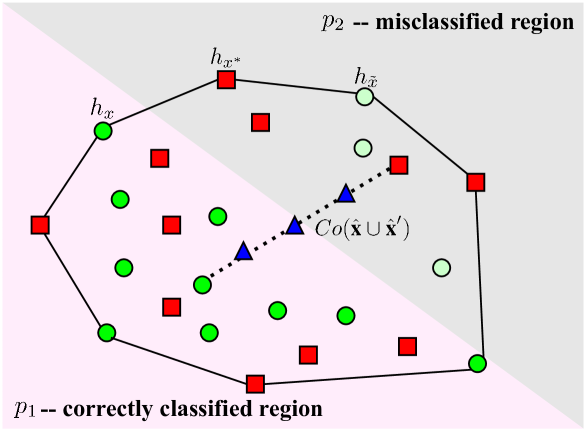
Figure 2: The schematic diagram of the data classification region and the convex hull.

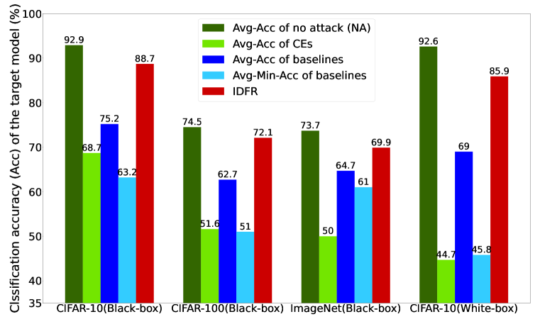
Figure 3: The statistical average performances of the proposed IDFR and baselines.

Ablation Study In this paper, we mainly adopt the jointly enhanced strategy of the input denoising (ID) and the hidden lossy feature restoring (FR) to improve the target model adversarial robustness. Table 5 shows the experiments (black-box attacks running 20 iterations with $l_{\infty}$ bounded and $\epsilon$=4/8/16 on target model ResNet50) of our method for ablation study, i.e., without FR, denoted as ID, or with jointly enhanced strategy both the ID and FR, denoted as ID+FR, respectively. The experiments clearly show that: 1) the ID model has strong ability of the adversarial denoising regardless of datasets and AEs. For example, our ID improves the adversarial robustness of the target model by 34% to 85% in terms of various AEs, 2) the FR enhances the adversarial robustness by 0.4% to 16.8% against various adversarial attacks, which fully verifies the necessity and importance of the FR, and 3) the jointly enhanced strategy of the ID+FR achieves: (1) improved the target model adversarial robustness with a large margin, and (2) the increase tends of the model’s defense performance with the increase of the adversarial attack powers, i.e., when $\epsilon$ increases.

Table 5: The ablation experimental results on ResNet50

Defense	FGSM($\epsilon=4/8/16$)		CW($\epsilon=4/8/16$)
Method	CIFAR10	SVHN	CIFAR10	SVHN
No Defense	52.7/44.0/34.0	52.1/40.0/27.4	17.1/14.2/ 9.0	37.1/17.2/ 9.5
ID	86.7/90.5/92.2	92.6/95.3/96.1	81.8/82.1/73.2	95.8/93.5/94.6
ID+FR	88.3/91.5/93.4	93.5/96.2/97.4	85.0/85.2/90.0	96.2/94.8/95.7

5 Conclusion

In this study, to address the weakness of existing adversarial defense methods, for the first time, we introduced the formal and complete problem definition for the defense against adversarial attacks, and reveal the acoustic disaster, i.e., the decrease of the target model’s robustness due to the damaged clean samples caused by the AEs denoising. On the above basis, we presented a novel enhanced adversarial defense method, namely IDFR, which consists of an enhanced input denoiser ID and an efficient hidden lossy feature restorer FR with the convex hull optimization. Extensive experimental results have verified the effectiveness of the proposed IDFR, and have clearly shown that the IDFR has achieved a new SOTA adversarial defense robustness performance compared to many state-of-the-art adversarial attack defense methods. How to further improve the defense performance of the proposed IDFR is our future research direction.

Appendix A Appendix

A.1 The network architectures of the proposed ID and FR

In this paper, we introduce the U-Net convolutional network (Ronneberger et al., 2015) as the basic network model of our proposed ID. The structure and hyperparameters of the ID are shown in Table 6. The ID consists of 7 layers CNN, the outputs of the 3th layer and the 5th layer are connected to the input of the 6th layer, respectively. Similarly, the outputs of the 2th layer the 7th layer are connected to the input of the 8th layer, respectively.

Similarly, as we discussed earlier, our FR model also uses the U-Net network model. The FR model consists of 6 layers fully connected networks as shown in Table 7.

Table 6: Hyperparameters of the ID Layers

layer	type	output channels	input channels	filter size
1st layer	conv+BN+ReLU	32	3	3 $\times$ 3
2nd layer	conv+BN+ReLU	32	32	3 $\times$ 3
3rd layer	conv+BN+ReLU	64	32	3 $\times$ 3
4th layer	conv+BN+ReLU	64	64	3 $\times$ 3
5th layer	conv+BN+ReLU	128	64	3 $\times$ 3
6th layer	conv+BN+ReLU	192	192	3 $\times$ 3
7th layer	conv+BN+ReLU	64	192	3 $\times$ 3
8th layer	conv+BN+ReLU	96	96	3 $\times$ 3
9th layer	conv+BN+ReLU	3	96	3 $\times$ 3

Table 7: Hyperparameters of the FR Layers

layer	type	output dimensions	input dimensions
1st layer	Fully Connect+ReLU	256	512
2nd layer	Fully Connect+ReLU	128	256
3rd layer	Fully Connect+ReLU	32	128
4th layer	Fully Connect+ReLU	128	32
5th layer	Fully Connect+ReLU	256	128
6th layer	Fully Connect+ReLU	512	256

A.2 Proof of Theorem 1

Proof.

For the Theorem 1, it is equal to the problem: given a convex hull $Co(\hat{\textbf{x}}\cup\hat{\textbf{x}}^{\prime})$, for any positive integer $n\geq 2$, $\forall h_{1},h_{2},\cdots,h_{n}\in Co(\hat{\textbf{x}}\cup\hat{\textbf{x}}^{\prime})$, given any non-negative real number $\alpha_{1},\alpha_{2},\cdots,\alpha_{n}$ and $\alpha_{1}+\alpha_{2}+\cdots+\alpha_{n}=1$, there is a constant $\alpha_{1}h_{1}+\alpha_{2}h_{2}+\cdots+\alpha_{n}h_{n}\in Co(\hat{\textbf{x}}\cup\hat{\textbf{x}}^{\prime})$.

Next, we prove Theorem 1 by mathematical induction:

By Eq. 4, the Theorem 1 holds when $n=2$.

Assume that the conclusion holds for $n=k$ points, and now we must prove that the conclusion holds for $n=k+1$ points.

$$\because\forall\alpha_{i}\geq 0,\sum_{i=1}^{k+1}\alpha_{i}=1,\forall h_{1},h_{2},\cdots,h_{n}\in Co(\hat{\textbf{x}}\cup\hat{\textbf{x}}^{\prime})$$ (7)

Then, when $\sum_{i=1}^{k}\alpha_{i}=0$ and $\alpha_{k+1}=1$, we have

$$h_{k+1}\in Co(\hat{\textbf{x}}\cup\hat{\textbf{x}}^{\prime})$$ (8)

$\because$ when $\sum_{i=1}^{k}\alpha_{i}\neq 0$,

$$\alpha_{1}h_{1}+ \alpha_{2}h_{2}+\cdots+\alpha_{k+1}h_{k+1}=$$ (9)

$$\Bigl{(}\sum_{i=1}^{k}\alpha_{i}\Bigl{[}\frac{\alpha_{1}}{\sum_{i=1}^{k}\alpha_{i}}h_{1}+\frac{\alpha_{2}}{\sum_{i=1}^{k}\alpha_{i}}h_{2}+\cdots+\frac{\alpha_{k}}{\sum_{i=1}^{k}\alpha_{i}}h_{k}\Bigr{]}+\alpha_{k+1}h_{k+1}\Bigr{)}$$

As the conclusion holds assuming for $n=k$ points, i.e., following Eq. 9 holds

$$\Bigl{(}\sum_{i=1}^{k}\alpha_{i}\Bigl{[}\frac{\alpha_{1}}{\sum_{i=1}^{k}\alpha_{i}}h_{1}+\frac{\alpha_{2}}{\sum_{i=1}^{k}\alpha_{i}}h_{2}+\cdots+\frac{\alpha_{k}}{\sum_{i=1}^{k}\alpha_{i}}h_{k}\Bigr{]}\Bigr{)}\in Co(\hat{\textbf{x}}\cup\hat{\textbf{x}}^{\prime})$$ (10)

$\because\alpha_{k+1}h_{k+1}\in Co(\hat{\textbf{x}}\cup\hat{\textbf{x}}^{\prime})$, $\sum_{i=1}^{k}\alpha_{i}\geq 0,\alpha_{k+1}\geq 0,\text{and}\sum_{i=1}^{k}\alpha_{i}+\alpha_{k+1}=1$.

Based on Eqs 8 and 10, with the basic definition of a convex set, we can get the following Eq. 11.

$$\alpha_{1}h_{1}+\alpha_{2}h_{2}+\cdots+\alpha_{n}h_{n}\in Co(\hat{\textbf{x}}\cup\hat{\textbf{x}}^{\prime}),n=k+1$$ (11)

∎

References

- Amodei et al. (2016) Dario Amodei, Chris Olah, Jacob Steinhardt, Paul Christiano, John Schulman, and Dan Mané. Concrete problems in ai safety. arXiv preprint arXiv:1606.06565, 2016.
- Biggio et al. (2013) Battista Biggio, Igino Corona, Davide Maiorca, Blaine Nelson, Nedim Srndic, Pavel Laskov, Giorgio Giacinto, and Fabio Roli. Evasion attacks against machine learning at test time. In Machine Learning and Knowledge Discovery in Databases - European Conference, ECML PKDD 2013, Prague, Czech Republic, September 23-27, 2013, Proceedings, Part III, pp. 387–402, 2013.
- Boyd et al. (2004) Stephen Boyd, Stephen P Boyd, and Lieven Vandenberghe. Convex optimization. Cambridge university press, 2004.
- Carlini & Wagner (2017) Nicholas Carlini and David A. Wagner. Towards evaluating the robustness of neural networks. In 2017 IEEE Symposium on Security and Privacy, SP 2017, San Jose, CA, USA, May 22-26, 2017, pp. 39–57, 2017.
- Chen et al. (2020a) Kai Chen, Haoqi Zhu, Leiming Yan, and Jinwei Wang. A survey on adversarial examples in deep learning. Journal on Big Data, 2(2):71–84, 2020a.
- Chen et al. (2020b) Tianlong Chen, Sijia Liu, Shiyu Chang, Yu Cheng, Lisa Amini, and Zhangyang Wang. Adversarial robustness: From self-supervised pre-training to fine-tuning. In 2020 IEEE/CVF Conference on Computer Vision and Pattern Recognition (CVPR), pp. 696–705, 2020b.
- Deng et al. (2009) Jia Deng, Wei Dong, Richard Socher, Li-Jia Li, Kai Li, and Li Fei-Fei. Imagenet: A large-scale hierarchical image database. In 2009 IEEE Conference on Computer Vision and Pattern Recognition, pp. 248–255, 2009.
- Ding et al. (2020) Gavin Weiguang Ding, Yash Sharma, Kry Yik Chau Lui, and Ruitong Huang. MMA training: Direct input space margin maximization through adversarial training. In 8th International Conference on Learning Representations, ICLR 2020, 2020.
- Gokhale et al. (2021) Tejas Gokhale, Rushil Anirudh, Bhavya Kailkhura, Jayaraman J. Thiagarajan, Chitta Baral, and Yezhou Yang. Attribute-guided adversarial training for robustness to natural perturbations. In Thirty-Fifth AAAI Conference on Artificial Intelligence, AAAI 2021, pp. 7574–7582, 2021.
- Goodfellow et al. (2015) Ian J. Goodfellow, Jonathon Shlens, and Christian Szegedy. Explaining and harnessing adversarial examples. In Yoshua Bengio and Yann LeCun (eds.), 3rd International Conference on Learning Representations, ICLR 2015, 2015.
- Gu & Rigazio (2015) Shixiang Gu and Luca Rigazio. Towards deep neural network architectures robust to adversarial examples. In Yoshua Bengio and Yann LeCun (eds.), 3rd International Conference on Learning Representations, ICLR 2015, 2015.
- Guo et al. (2018) Chuan Guo, Mayank Rana, Moustapha Cissé, and Laurens van der Maaten. Countering adversarial images using input transformations. In 6th International Conference on Learning Representations, ICLR 2018, 2018.
- He et al. (2016) Kaiming He, Xiangyu Zhang, Shaoqing Ren, and Jian Sun. Deep residual learning for image recognition. In 2016 IEEE Conference on Computer Vision and Pattern Recognition, 2016, pp. 770–778, 2016.
- Hendrycks et al. (2019) Dan Hendrycks, Mantas Mazeika, Saurav Kadavath, and Dawn Song. Using self-supervised learning can improve model robustness and uncertainty. In Advances in Neural Information Processing NeurIPS 2019, pp. 15637–15648, 2019.
- Jeong & Shin (2020) Jongheon Jeong and Jinwoo Shin. Consistency regularization for certified robustness of smoothed classifiers. In Hugo Larochelle, Marc’Aurelio Ranzato, Raia Hadsell, Maria-Florina Balcan, and Hsuan-Tien Lin (eds.), Advances in Neural Information Processing Systems 33: Annual Conference on Neural Information Processing Systems 2020, NeurIPS 2020, December 6-12, 2020, virtual, 2020.
- Jia & Liang (2017) Robin Jia and Percy Liang. Adversarial examples for evaluating reading comprehension systems. In Proceedings of the 2017 Conference on Empirical Methods in Natural Language Processing, EMNLP 2017, pp. 2021–2031, 2017.
- Jia et al. (2019) Xiaojun Jia, Xingxing Wei, Xiaochun Cao, and Hassan Foroosh. Comdefend: An efficient image compression model to defend adversarial examples. In IEEE Conference on Computer Vision and Pattern Recognition, CVPR 2019, pp. 6084–6092, 2019.
- Joshi et al. (2019) Ameya Joshi, Amitangshu Mukherjee, Soumik Sarkar, and Chinmay Hegde. Semantic adversarial attacks: Parametric transformations that fool deep classifiers. In Proceedings of the IEEE/CVF International Conference on Computer Vision, pp. 4773–4783, 2019.
- Kos et al. (2018) Jernej Kos, Ian Fischer, and Dawn Song. Adversarial examples for generative models. In 2018 IEEE Security and Privacy Workshops, SP Workshops 2018, pp. 36–42, 2018.
- Krizhevsky et al. (2009) Alex Krizhevsky, Geoffrey Hinton, et al. Learning multiple layers of features from tiny images. 2009.
- Kurakin et al. (2017) Alexey Kurakin, Ian J. Goodfellow, and Samy Bengio. Adversarial examples in the physical world. In 5th International Conference on Learning Representations, ICLR 2017, 2017.
- LeCun et al. (1998) Yann LeCun, Léon Bottou, Yoshua Bengio, and Patrick Haffner. Gradient-based learning applied to document recognition. Proceedings of the IEEE, 86(11):2278–2324, 1998.
- Liao et al. (2018) Fangzhou Liao, Ming Liang, Yinpeng Dong, Tianyu Pang, Xiaolin Hu, and Jun Zhu. Defense against adversarial attacks using high-level representation guided denoiser. In 2018 IEEE Conference on Computer Vision and Pattern Recognition, CVPR 2018, pp. 1778–1787, 2018.
- Liu & Deng (2015) Shuying Liu and Weihong Deng. Very deep convolutional neural network based image classification using small training sample size. In 3rd IAPR Asian Conference on Pattern Recognition, ACPR 2015, pp. 730–734, 2015.
- Liu et al. (2021) Xiaolei Liu, Xingshu Chen, Mingyong Yin, Yulong Wang, Teng Hu, and Kangyi Ding. Audio injection adversarial example attack. In ICML 2021 Workshop on Adversarial Machine Learning, 2021.
- Machado et al. (2020) Gabriel Resende Machado, Eugênio Silva, and Ronaldo Ribeiro Goldschmidt. Adversarial machine learning in image classification: A survey towards the defender’s perspective. arXiv preprint arXiv:2009.03728, 2020.
- Madry et al. (2018) Aleksander Madry, Aleksandar Makelov, Ludwig Schmidt, Dimitris Tsipras, and Adrian Vladu. Towards deep learning models resistant to adversarial attacks. In 6th International Conference on Learning Representations, ICLR 2018, 2018.
- Mao et al. (2019) Chengzhi Mao, Ziyuan Zhong, Junfeng Yang, Carl Vondrick, and Baishakhi Ray. Metric learning for adversarial robustness. In Advances in Neural Information Processing Systems NeurIPS 2019, pp. 478–489, 2019.
- Naseer et al. (2020) Muzammal Naseer, Salman H. Khan, Munawar Hayat, Fahad Shahbaz Khan, and Fatih Porikli. A self-supervised approach for adversarial robustness. In 2020 IEEE/CVF Conference on Computer Vision and Pattern Recognition, CVPR 2020, pp. 259–268, 2020.
- Netzer et al. (2011) Yuval Netzer, Tao Wang, Adam Coates, Alessandro Bissacco, Bo Wu, and Andrew Y Ng. Reading digits in natural images with unsupervised feature learning. 2011.
- Pang et al. (2020) Tianyu Pang, Kun Xu, Yinpeng Dong, Chao Du, Ning Chen, and Jun Zhu. Rethinking softmax cross-entropy loss for adversarial robustness. In 8th International Conference on Learning Representations, ICLR 2020, 2020.
- Papernot et al. (2016a) Nicolas Papernot, Patrick McDaniel, and Ian Goodfellow. Transferability in machine learning: from phenomena to black-box attacks using adversarial samples, 2016a.
- Papernot et al. (2016b) Nicolas Papernot, Patrick D. McDaniel, Xi Wu, Somesh Jha, and Ananthram Swami. Distillation as a defense to adversarial perturbations against deep neural networks. In IEEE Symposium on Security and Privacy, SP 2016, pp. 582–597, 2016b.
- Papernot et al. (2017) Nicolas Papernot, Patrick D. McDaniel, Ian J. Goodfellow, Somesh Jha, Z. Berkay Celik, and Ananthram Swami. Practical black-box attacks against machine learning. In Proceedings of the 2017 ACM on Asia Conference on Computer and Communications Security, 2017, pp. 506–519, 2017.
- Qi et al. (2021) Gege Qi, Lijun Gong, Yibing Song, Kai Ma, and Yefeng Zheng. Stabilized medical image attacks. In 9th International Conference on Learning Representations, ICLR 2021, 2021.
- Ronneberger et al. (2015) Olaf Ronneberger, Philipp Fischer, and Thomas Brox. U-net: Convolutional networks for biomedical image segmentation. In Medical Image Computing and Computer-Assisted Intervention - MICCAI, volume 9351 of Lecture Notes in Computer Science, pp. 234–241. Springer, 2015.
- Samangouei et al. (2018) Pouya Samangouei, Maya Kabkab, and Rama Chellappa. Defense-gan: Protecting classifiers against adversarial attacks using generative models. In 6th International Conference on Learning Representations, ICLR 2018, 2018.
- Shafahi et al. (2019a) Ali Shafahi, W. Ronny Huang, Christoph Studer, Soheil Feizi, and Tom Goldstein. Are adversarial examples inevitable? In 7th International Conference on Learning Representations, ICLR 2019, 2019a.
- Shafahi et al. (2019b) Ali Shafahi, Mahyar Najibi, Amin Ghiasi, Zheng Xu, John P. Dickerson, Christoph Studer, Larry S. Davis, Gavin Taylor, and Tom Goldstein. Adversarial training for free! In Advances in Neural Information Processing Systems, NeurIPS 2019, pp. 3353–3364, 2019b.
- Shi et al. (2021) Changhao Shi, Chester Holtz, and Gal Mishne. Online adversarial purification based on self-supervised learning. In 9th International Conference on Learning Representations, ICLR 2021, 2021.
- Song et al. (2018) Yang Song, Taesup Kim, Sebastian Nowozin, Stefano Ermon, and Nate Kushman. Pixeldefend: Leveraging generative models to understand and defend against adversarial examples. In 6th International Conference on Learning Representations, ICLR 2018, 2018.
- Stutz et al. (2020) David Stutz, Matthias Hein, and Bernt Schiele. Confidence-calibrated adversarial training: Generalizing to unseen attacks. In Proceedings of the 37th International Conference on Machine Learning, ICML 2020, pp. 9155–9166, 2020.
- Szegedy et al. (2014) Christian Szegedy, Wojciech Zaremba, Ilya Sutskever, Joan Bruna, Dumitru Erhan, Ian J. Goodfellow, and Rob Fergus. Intriguing properties of neural networks. 2014.
- Szegedy et al. (2016) Christian Szegedy, Vincent Vanhoucke, Sergey Ioffe, Jonathon Shlens, and Zbigniew Wojna. Rethinking the inception architecture for computer vision. In 2016 IEEE Conference on Computer Vision and Pattern Recognition, 2016, pp. 2818–2826, 2016.
- Tramèr et al. (2020) Florian Tramèr, Alexey Kurakin, Nicolas Papernot, Ian Goodfellow, Dan Boneh, and Patrick McDaniel. Ensemble adversarial training: Attacks and defenses. arXiv preprint arXiv:1705.07204, 2020.
- Vincent et al. (2008) Pascal Vincent, Hugo Larochelle, Yoshua Bengio, and Pierre-Antoine Manzagol. Extracting and composing robust features with denoising autoencoders. In Proceedings of the 25th International Conference on Machine Learning, ICML, pp. 1096–1103, 2008.
- Wang et al. (2020) Yisen Wang, Difan Zou, Jinfeng Yi, James Bailey, Xingjun Ma, and Quanquan Gu. Improving adversarial robustness requires revisiting misclassified examples. In 8th International Conference on Learning Representations, ICLR 2020, 2020.
- Warde-Farley & Goodfellow (2016) David Warde-Farley and Ian Goodfellow. 11 adversarial perturbations of deep neural networks. Perturbations, Optimization, and Statistics, 311, 2016.
- Wong et al. (2020) Eric Wong, Leslie Rice, and J. Zico Kolter. Fast is better than free: Revisiting adversarial training. In 8th International Conference on Learning Representations, ICLR 2020, 2020.
- Xu et al. (2018) Weilin Xu, David Evans, and Yanjun Qi. Feature squeezing: Detecting adversarial examples in deep neural networks. In 25th Annual Network and Distributed System Security Symposium, NDSS 2018, 2018.
- Yoon et al. (2021) Jongmin Yoon, Sung Ju Hwang, and Juho Lee. Adversarial purification with score-based generative models. In Proceedings of the 38th International Conference on Machine Learning, ICML 2021, pp. 12062–12072, 2021.
- Yuan et al. (2019) Xiaoyong Yuan, Pan He, Qile Zhu, and Xiaolin Li. Adversarial examples: Attacks and defenses for deep learning. IEEE Trans. Neural Networks Learn. Syst., 30(9):2805–2824, 2019.
- Zhang et al. (2018) Hongyi Zhang, Moustapha Cissé, Yann N. Dauphin, and David Lopez-Paz. mixup: Beyond empirical risk minimization. In 6th International Conference on Learning Representations, ICLR 2018, 2018.
- Zhang & Li (2020) Jiliang Zhang and Chen Li. Adversarial examples: Opportunities and challenges. IEEE Transactions on Neural Networks and Learning Systems, 31(7):2578–2593, 2020.
- Zheng et al. (2020) Haizhong Zheng, Ziqi Zhang, Juncheng Gu, Honglak Lee, and Atul Prakash. Efficient adversarial training with transferable adversarial examples. In 2020 IEEE/CVF Conference on Computer Vision and Pattern Recognition, CVPR 2020, pp. 1178–1187, 2020.
- Zhou et al. (2021) Yi Zhou, Xiaoqing Zheng, Cho-Jui Hsieh, Kai-Wei Chang, and Xuanjing Huang. Defense against synonym substitution-based adversarial attacks via dirichlet neighborhood ensemble. In Proceedings of the 59th Annual Meeting of the Association for Computational Linguistics and the 11th International Joint Conference on Natural Language Processing, ACL/IJCNLP 2021, pp. 5482–5492, 2021.