Physical and Geometrical Parameters of the Evolved Binary System HD6009

Abstract

Atmospheric modeling and dynamical analysis of the components of the visually close binary system (VCBS) HD6009 were used to estimate their individual physical and geometrical parameters. Model atmospheres were constructed using a grid of Kurucz solar metalicity blanketed models, and used to compute the individual synthetic spectral energy distribution (SED) for each component separately. These SEDs were combined together to compute the entire SED for the system from the net luminosities of the components $a$ and $b$ located at a distance $d$ from the Earth. We used the feedback modified parameters and iteration method to get the best fit between synthetic and observational entire SEDs.

The physical and geometrical parameters of the system’s components were derived as: $T_{\rm eff}^{a}=5625\pm 75$ K, $T_{\rm eff}^{b}=5575\pm 75$ K, log $g_{a}=3.75\pm 0.25$, log $g_{b}=3.75\pm 0.25$, $R_{a}=2.75\pm 0.30R_{\odot}$, $R_{b}=2.65\pm 0.30R_{\odot}$, $M_{v}^{a}=2\hbox{$.\!\!^{m}$}80\pm 0.30$, $M_{v}^{b}=2\hbox{$.\!\!^{m}$}93\pm 0.30$, $M_{a}=1.42\pm 0.15M_{\odot}$, $M_{b}=1.40\pm 0.15M_{\odot}$, $L_{a}=6.80\pm 0.75L_{\odot}$, $L_{b}=6.09\pm 0.75L_{\odot}$ and $\pi=14.43$mas dynamical parallax. The system is shown to be consist of G6 IV primary and G6 IV secondary components.

I Introduction

Hipparcos mission revealed that many of the previously known as single stars are actually binary or multiple systems, rasing by that the duplicity and multiplicity of galactic stellar systems. Most of these binary and multiple systems are nearby stars, which appears as a single star even with largest ground based telescopes except by means of modern high resolution techniques like speckle interferometry (SI) and adaptive optics (AO). These systems are known as visually close (spatially unresolved on the sky) binary systems (VCBS).

The study of binary systems, in general, plays an important role in determining several key stellar parameters, which is more complicated in the case of the evolved VCBS. In spite the fact that hundreds of binary systems with periods in the order of 10 years or less, are routinely observed by different groups of high resolution techniques around the world, there is still a lake in the determination of the individual physical parameters of the systems’ components. So, the combination of speckle interferometry, spectrophotometry, atmospheres modelling and -recently- orbital analysis opens a new window in the accurate determination of the physical and geometrical parameters of VCBS. These parameters include the effective temperatures, radii, orbital elements, spectral types, luminosity classes and masses for both components of the binary system. The method was successfully applied to several main sequence binary systems: ADS11061, Cou1289, Cou1291, Hip11352, Hip11253, Hip70973 and Hip72479 (Al-Wardat, 2002a, 2007, 2009; Al-Wardat & Widyan, 2009; Al-Wardat, 2012), and to the subgiant systems HD25811 and HD375 (Al-Wardat et al., 2013b, a).

The system HD6009 (Hip4809) is a well known VCB, which is routinely observed by different SI groups around the world. It was first proposed as an evolved G9 star with luminosity class between III and IV by Yoss (1961) from his analysis of the strength of the $\lambda$4077 ionized strontium line based on the prism spectra from the Curtis Schmidt telescope of the University of Michigan and slit spectrograms from the 60 inch reflector of the Mt. Wilson Observatory, which was supported as IV by the moderate cyanogen absorption at $\lambda$4216. Balega et al. (2002) also noted that the computed absolute magnitudes of the individual components as $M_{va}=3.1\&M_{vb}=3.3$ with their late G spectral type do not correspond to their ($B-V$)or ($V-I$) colours, which means that the system is evolved. Moreover, Balega et al. (2006b) found that the system consists of G6 and G9 subgiant stars depending on the magnitude difference and Hipparcos parallax measurements.

So, the analysis of the system the aforementioned method would help in understanding the formation and evolution mechanisms of stellar binary systems.

Table  1contains the SIMBAD data of the system, and Table  2 contains data from Hipparcos and Tycho Catalogues (ESA, 1997).

Table 1: Data from SIMBAD

	HD6009
	Hip4809
$\alpha_{2000}$	$01^{h}01^{m}43\hbox{$.\!\!^{s}$}581$
$\delta_{2000}$	$+25\hbox{${}^{\circ}$}17^{\prime}31.^{\prime\prime}99$
Tyc	1743-1174-1
HD	6009
Spectral type	G8IV

Table 2: Data from Hipparcos and Tycho Catalogues

	HD6009
	Hip4809
$V_{J}(Hip)$	$6\hbox{$.\!\!^{m}$}71$
$B_{T}$	$7\hbox{$.\!\!^{m}$}683\pm 0.008$
$V_{T}$	$6\hbox{$.\!\!^{m}$}806\pm 0.006$
$(B-V)_{J}(Tycho)$	$0\hbox{$.\!\!^{m}$}783\pm 0.007$
Hip Trig. Parallax (mas)	$13.94\pm 0.90$
Tyc Trig. Parallax (mas)	$12.3\pm 5.3$

Table 3 lists the synthetic Jonson, Strömgren and Tycho magnitudes and color indices, which were calculated by Al-Wardat (2002b, 2008), depending on the observational SED.

Table 3: Jonson, Strömgren and Tycho magnitudes and color indices of the entire system Al-Wardat (2002b, 2008).

	HD6009
	Hip4809
$B_{J}$	$7\hbox{$.\!\!^{m}$}43\pm 0.06$
$R_{J}$	$6\hbox{$.\!\!^{m}$}32\pm 0.07$
$V_{J}$	$6\hbox{$.\!\!^{m}$}74\pm 0.06$
$(B-V)_{J}$	$0\hbox{$.\!\!^{m}$}67\pm 0.08$
$v$	$7\hbox{$.\!\!^{m}$}85\pm 0.06$
$b$	$7\hbox{$.\!\!^{m}$}145\pm 0.06$
$y$	$6\hbox{$.\!\!^{m}$}70\pm 0.06$
$v-b$	$0\hbox{$.\!\!^{m}$}72\pm 0.08$
$b-y$	$0\hbox{$.\!\!^{m}$}44\pm 0.08$
$B_{T}$	$7\hbox{$.\!\!^{m}$}64\pm 0.06$
$V_{T}$	$6\hbox{$.\!\!^{m}$}81\pm 0.06$
$(B-V)_{T}$	$0\hbox{$.\!\!^{m}$}82\pm 0.08$

II ORBITAL ELEMENTS

Balega et al. (2006a) introduced a preliminary orbit of the system depending on 12 interferometric measurements and the first Hipparcos data point with a period of about 15 years. The orbit was then modified by Balega et al. (2006b) using 16 astrometric measurements (black dots in Fig.  2).

A slight modification of the orbit is introduced here using all relative positional measurements listed in Table  5, which includes 12 more measurements than those used by Balega et al. (2006b) and cover the complete orbit since the first measurement of Hipparcos (Fig.  2). The quadrants of some of these measurements were adjusted to obtain a consistent orbit.

Table 4: Modified orbital elements of the system with those of the old orbit by (Balega et al., 2006b).

Parameters	This work	Old orbit by (Balega et al., 2006b) $\dagger$
Period $P$	$16.28^{y}\pm 0.08^{y}$	$16.41^{y}\pm 0.11^{y}$
Periastron epoch $T_{0}$	$1998.55\pm 0.06$	$1998.62\pm 0.02$
Eccentricity $e$	$0.385\pm 0.014$	$0.393\pm 0.012$
Semi-major axis $a$	$0\hbox{$.\!\!^{\prime\prime}$}130\pm 0.002$	$0\hbox{$.\!\!^{\prime\prime}$}128\pm 0.002$
Inclination $i$	$58.18^{\circ}\pm 0.93$	$58.4^{\circ}\pm 0.5$
Argument of periastron $\omega$	$287.45^{\circ}\pm 0.60$	$106.9^{\circ}\pm 0.6$
Position angle of nodes $\Omega$	$235.03^{\circ}\pm 0.68$	$57.1^{\circ}\pm 0.8$

The estimated orbital elements of the system along with those of the old orbit are listed in Table  4.

Fig.  1 shows the relative visual orbit of the system with the epoch of the positional measurements, and Fig.  2 shows the new orbit against the old one of (Balega et al., 2006b).

Table 5: Relative positional measurements using different methods which are used to build the orbit of the system. These points are taken from the Fourth Catalog of Interferometric Measurements of Binary Stars.

Date	$\theta$(deg)	$\sigma_{\theta}$	$\rho$(deg)	$\sigma_{\rho}$	$\triangle m$	$\sigma_{\triangle m}$	filter($\lambda$)	$\Delta\lambda$)	Tel.	Ref.†	Meth.‡
1991.25	188	1.5	0.118	0.004	0.28	0.30	511	222	0.3	HIP1997a ESA (1997)	Hh
1997.7206				$<$0.065			550	24	2.1	Msn1999b Mason et al. (1999)	Su
1998.7718	0	0	0	0	0.1	0.24	545	30	6	Plz2005 Pluzhnik (2005)	S
1998.7718	189.5	0.5	0.05	0.002	0.17	0.15	545	30	6	Bag2002 Balega et al. (2002)	S
1999.7472	228.2	1.5	0.086	0.002	0.3	0.16	2115	214	6	Bag2002 Balega et al. (2002)	S
1999.8128	49.5	0.3	0.0885	0.0003	0.19	0.04	610	20	6	Bag2004 Balega et al. (2004)	S
1999.8233	49.7	0	0.094	0	0	0	550	24	2.1	Msn2001b Mason et al. (2001)	Su
1999.8882	0	0	0	0	0.05	0.15	648	41	3.5	Hor2004 Horch et al. (2004)	S
1999.8882	52.5	0	0.089	0	0	0	648	41	3.5	Hor2002a Horch et al. (2002)	S
2000.7674	0	0	0	0	0.22	0.15	503	40	3.5	Hor2004 Horch et al. (2004)	S
2000.7674	65.5	0	0.107	0	0	0	503	40	3.5	Hor2002a Horch et al. (2002)	S
2000.8728	249.2	0.6	0.106	0.001	0.12	0.19	800	110	6	Bag2006b Balega et al. (2006a)	S
2000.8755	248.8	0.4	0.106	0.001	0.16	0.05	600	30	6	Bag2006b Balega et al. (2006a)	S
2001.7526	261.9	0.2	0.107	0.001	0	0.12	545	30	6	Bag2006b Balega et al. (2006a)	S
2001.7526	262.2	0.2	0.107	0.001	0	0.12	600	30	6	Bag2006b Balega et al. (2006a)	S
2001.753	262.2	0	0.107	0	0	0	–	–	6	Bag2006 Balega et al. (2006b)	S
2001.845	263.1	0	0.107	0	0	0	–	–	6	Bag2006 Balega et al. (2006b)	S
2002.726	275.2	0	0.103	0	0	0	–	–	6	Bag2006 Balega et al. (2006b)	S
2002.796	278.6	0	0.1	0	0	0	–	–	6	Bag2006 Balega et al. (2006b)	S
2003.6372	109.2	0	0.095	0	0	0	550	40	3.5	Hor2008 Horch et al. (2008)	S
2003.6372	112.5	0	0.095	0	0.15	0	754	44	3.5	Hor2008 Horch et al. (2008)	S
2003.6372	113.2	0	0.094	0	0	0	698	39	3.5	Hor2008 Horch et al. (2008)	S
2003.6372	293.2	0	0.096	0	0	0	650	38	3.5	Hor2008 Horch et al. (2008)	S
2003.928	299.9	0	0.092	0	0	0	–	–	6	Bag2006 Balega et al. (2006b)	S
2004.815	318.7	0	0.09	0	0	0	–	–	6	Bag2006 Balega et al. (2006b)	S
2004.8154	318.8	0.3	0.089	0.002	0.21	0.04	600	30	6	Bag2007bBalega et al. (2007)	S
2005.5619	338	0	0.098	0	0.81	0	698	39	3.5	Hor2008 Horch et al. (2008)	S
2005.5975	337.6	0	0.092	0	0.06	0	698	39	3.5	Hor2008 Horch et al. (2008)	S
2005.5975	336.7	0	0.092	0	0	0	698	39	3.5	Hor2008 Horch et al. (2008)	S
2005.8627	339.7	0	0.106	0	0	0	550	24	3.8	Msn2009 Mason et al. (2009)	Su
2007.8228	192	0	0.116	0	0.26	0	698	39	3.5	Hor2010 Horch et al. (2010)	S
2008.702	201.8	1.1	0.127	0.003	0	0.12	550	40	3.5	Hor2012a Horch et al. (2012)	S
2010.0045	214.8	0	0.138	0	0.23	0	562	40	3.5	Hor2011 Horch et al. (2011)	S
2010.0045	0	0	0	0	0.15	0	692	40	3.5	Hor2011 Horch et al. (2011)	S

^†References are abbreviated as in the Fourth Catalog of Interferometric Measurements of Binary Stars.
^‡ S: Speckle Interferometry, Su: USNO speckle.

Figure 1: Relative visual orbit of the system with the epoch of the positional measurements; the origin represents the position of the primary component.

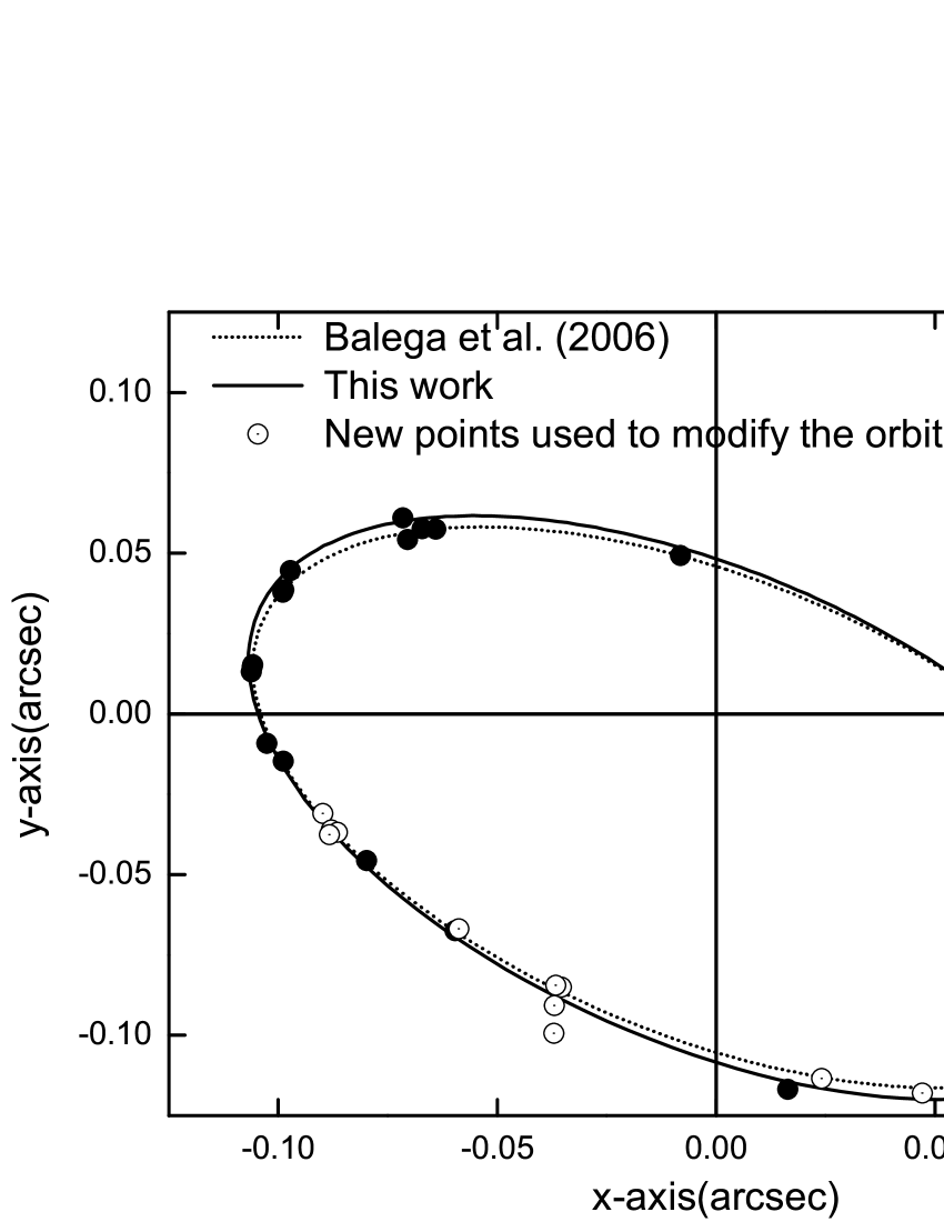
Figure 2: The modified relative visual orbit of the system in this work (solid line) against that of Balega et al. (2006b) (doted line).

III Atmospheric modelling

III.1 Input parameters for model atmospheres

Using $m_{v}=6\hbox{$.\!\!^{m}$}71$ from Table  2 and $\triangle m=0\hbox{$.\!\!^{m}$}18$ as the average of all 19 $\triangle m$ measurements (Table  5), since there is no significant difference in $\triangle m$ under different filters between $\lambda$503-800 nm, we calculated a preliminary individual $m_{v}$ for each component as: $m_{va}=7\hbox{$.\!\!^{m}$}376$ and $m_{vb}=7\hbox{$.\!\!^{m}$}556$.

These visual magnitudes along with the system’s parallax from Hipparcos catalogue ($\pi=13.94\pm 0.90,d=71.74pc$) and the extinction coefficient $A_{v}=0.1432$ mag from Schlafly & Finkbeiner (2011) and Galactic Dust Reddening and Extinction Archive (http://irsa.ipac.caltech.edu/applications/DUST/) with the following equation:

$$M_{v}=m_{v}+5-5\log(d)-A,$$ (1)

give the absolute individual magnitudes as:

$M_{v}^{a}=2\hbox{$.\!\!^{m}$}95$ and $M_{v}^{b}=3\hbox{$.\!\!^{m}$}13$.

So, the correspondent effective temperatures for such absolute magnitudes would be either $T_{\rm eff}^{a}=6950\rm{K}\,\,\&\,T_{\rm eff}^{b}=6800\rm{K}$ in the case of main sequence components as given by the Tables of Gray (2005) or less in the case of evolved components. Hence, the gravity acceleration constant at the surface of such stars would be log$g\leq 4.3$.

These values of the effective temperatures and gravity accelerations represent the preliminary input parameters for atmospheric modeling of both components, from which we compute their synthetic spectra.

III.2 Synthetic spectra

The spectral energy distributions in the continuous spectrum for each component is computed depending on solar abundance model atmospheres of each component using grids of Kurucz’s 1994 blanketed models (ATLAS9).

The total energy flux from a binary star is created from the net luminosity of the components $a$ and $b$ located at a distance $d$ from the Earth (Al-Wardat, 2012). So we can write:

$$F_{\lambda}\cdot d^{2}=H_{\lambda}^{a}\cdot R_{a}^{2}+H_{\lambda}^{b}\cdot R_{b}^{2},$$ (2)

from which

$$F_{\lambda}=(R_{a}^{2}/d)^{2}(H_{\lambda}^{a}+H_{\lambda}^{b}\cdot(R_{b}/R_{a})^{2}),$$ (3)

where $H_{\lambda}^{a}$ and $H_{\lambda}^{b}$ are the fluxes from a unit surface of the corresponding component. $F_{\lambda}$ here represents the entire SED of the system.

When we built synthetic SEDs using the aforementioned preliminary input parameters (Sec. III.1) and equations  2 &  3, and compared them with the observational SED, we found that there was no coincidence between them within the criteria of the best fit which are the maximum values of the absolute fluxes, the inclination of the continuum of the spectra, and the profiles of the absorption lines.

So, many attempts were made to achieve the best fit between the synthetic SEDs and the observational one using the iteration method of different sets of parameters according to the following equations:

$$\log(R/R_{\odot})=0.5\log(L/L_{\odot})-2\log(T/T_{\odot})$$ (4)

$$\log g=\log(M/M_{\odot})-2\log(R/R_{\odot})+4.43,$$ (5)

where $T_{\odot}=5777\rm{K}$ was used. But in all attempts of modeling the components as main sequence stars, there were disagreements between synthetic and observational SEDs in both; the inclination of the continuum (which represents the effective temperatures) and the absolute flux (which represents either the radii of the components or the parallax of the system).

The key parameters to get the best fit are the radii of the components, which should be bigger than what would be if they were main sequence stars (as proposed formerly), and the effective temperatures which should be lower. That means both components are evolved stars.

So, depending on that proposal, hundreds of models were built and compared with the observational SED tell the best fit was achieved using the following set of parameters (Fig.  3):

$$T_{\rm eff}^{a}=5625\pm 75{\rm K},T_{\rm eff}^{b}=5675\pm 75{\rm K},$$

$$\log g_{a}=3.75\pm 0.25,\log g_{b}=3.75\pm 0.25,$$

$$R_{a}=2.69\pm 0.30R_{\odot},$$

and

$$R_{b}=2.42\pm 0.30R_{\odot}.$$

Thus the luminosities follow as: $L_{a}=6.51\pm 0.75L_{\odot}$, and $L_{b}=5.45\pm 0.75L_{\odot}$.

To ensure the correlation between physical and geometrical parameters and to connect the dynamical analysis with the atmospheric modeling, we used Kepler’s equation:

$$\ (\frac{M_{a}+M_{b}}{M_{\odot}})(\pi^{3})=\frac{a^{3}}{p^{2}},$$ (6)

$$\ \frac{\sigma_{M}}{M}=\sqrt{(3\frac{\sigma_{\pi}}{\pi})^{2}+(3\frac{\sigma_{a}}{a})^{2}+(2\frac{\sigma_{p}}{p})^{2},}$$ (7)

where $(\frac{M_{a}+M_{b}}{M_{\odot}})$ is the mass sum of the two components in terms of solar mass, $\pi$ is the parallax of the system in arc seconds, $a$ is the semi-major axes in arc seconds and $p$ is the period in years.

Using the orbital elements of the system calculated in section 4 and $\pi=13.94\pm 0.90$ as given by Hipparcos (Table  2), the mass sum of the two components follows as:

$$(M_{a}+M_{b})/M_{\odot}=3.06\pm 0.59,$$ (8)

which disagrees with the masses estimated from the evolutionary tracks based on atmospheres modeling. So, fixing the right part of equation  6 and changing the values of the left part in an iterated way, ensures agreement between the masses of the components, their positions on the evolutionary tracks and the best fit between the synthetic and observational SED’s.

For stars with formerly estimated physical and geometrical parameters, this agreement is possible only for a system at a distance $d=69.31$ pc ($\pi=14.43$mas).

The final physical and geometrical parameters of the system are listed in Table 7, which represent the parameters of the system’s components within the error values of the measured quantities. Depending on the tables of Gray (2005) or Lang (1992), the spectral types of the components are estimated as G6 and G5 for primary and secondary components respectively.

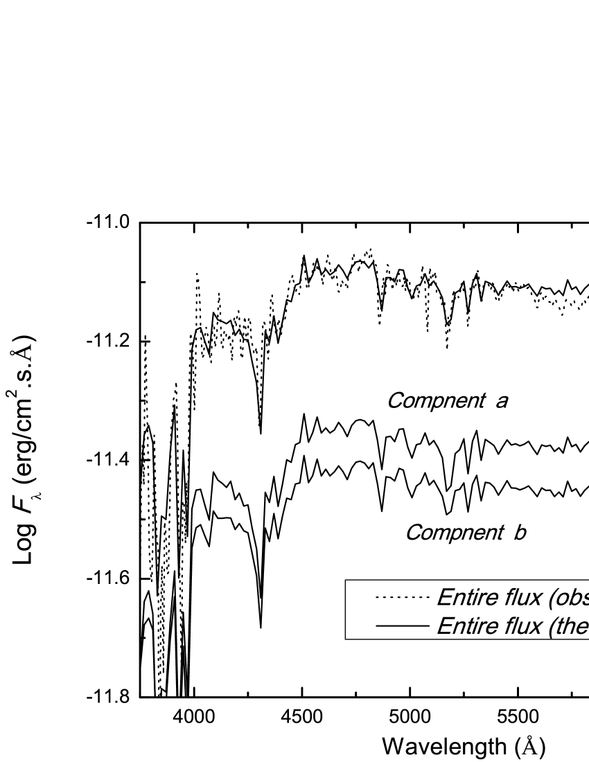
Figure 3: Dotted line: the entire observational SED in the continuous spectrum of the system (Al-Wardat, 2002b). Solid lines: the entire computed SED of the two components, the computed flux of the primary component with $T_{\rm eff}=5625\pm 75$ K, log $g=3.75\pm 0.25,R=2.69\pm 0.30R_{\odot}$, and the computed flux of the secondary component with $T_{\rm eff}=5675\pm 75$ K, log $g=3.75\pm 0.25$, $R=2.42\pm 0.30R_{\odot}$ and $d=69.31$ pc.

IV Synthetic photometry

In addition to the direct comparison, we can check reliability of our method of estimating the physical and geometrical parameters by comparing the observed magnitudes of the entire system from different ground or space based telescopes with the entire synthetic ones. For that, we used the following relation (Maíz Apellániz, 2006, 2007):

$$m_{p}[F_{\lambda,s}(\lambda)]=-2.5\log\frac{\int P_{p}(\lambda)F_{\lambda,s}(\lambda)\lambda{\rm d}\lambda}{\int P_{p}(\lambda)F_{\lambda,r}(\lambda)\lambda{\rm d}\lambda}+{\rm ZP}_{p}\,,$$ (9)

to calculate the entire and individual synthetic magnitudes of the system, where $m_{p}$ is the synthetic magnitude of the passband $p$, $P_{p}(\lambda)$ is the dimensionless sensitivity function of the passband $p$, $F_{\lambda,s}(\lambda)$ is the synthetic SED of the object and $F_{\lambda,r}(\lambda)$ is the SED of the reference star (Vega). Zero points (ZP_p) from Maíz Apellániz (2007) (and references there in) were adopted.

The results of the calculated magnitudes and color indices of the entire system and individual components, in different photometrical systems, are shown in Table 6.

Table 6: Magnitudes and color indices of the synthetic spectra of the system.

Sys.	Fil.	entire	comp. a	comp. b
Joh-	$U$	$7.72\pm 0.03$	$8.41$	$8.55$
Cou.	$B$	7.45	8.13	8.28
	$V$	6.71	7.38	7.56
	$R$	6.32	6.99	7.18
	$U-B$	0.28	0.29	0.27
	$B-V$	0.73	0.74	0.72
	$V-R$	0.39	0.40	0.38
Ström.	$u$	8.88	9.55	9.72
	$v$	7.84	8.52	8.66
	$b$	7.12	7.79	7.97
	$y$	6.68	7.35	7.53
	$u-v$	1.04	1.03	1.06
	$v-b$	0.72	0.73	0.70
	$b-y$	0.44	0.44	0.44
Tycho	$B_{T}$	7.64	8.32	8.46
	$V_{T}$	6.79	7.46	7.64
	$B_{T}-V_{T}$	0.84	0.86	0.83

V Results and discussion

A comparison between the synthetic magnitudes and colors (Table 6) with the observational ones (Tables 2 and 3) shows a very good consistency within the three photometrical systems Johnson-Cousins, Strömgren and Tycho. Also, synthetic visual magnitudes of the two components ( 6) fit exactly those calculated in section  III.1. This gives a good indication for the reliability of the method and the estimated parameters of the individual components of the system, which are listed in Table 7.

Moreover, there is a good consistency between the estimated absolute magnitudes as $M_{v}^{a}=2\hbox{$.\!\!^{m}$}80\pm 0.30,M_{v}^{b}=2\hbox{$.\!\!^{m}$}93\pm 0.30$ with those previously calculated in section  III.1 as $M_{v}^{a}=2\hbox{$.\!\!^{m}$}95,M_{v}^{b}=3\hbox{$.\!\!^{m}$}13$, and those given by Balega et al. (2002) as $M_{v}^{a}=3.1\&M_{v}^{b}=3.3$.

Dynamical parallax of the system is introduced here as $d=69.31$ pc ($\pi=14.43$mas), within the errors of Hipparcos parallax measurement, to insure the consistency between the physical and geometrical parameters, and to explain the R-L-T relation of such VCBS.

Fig. 4 shows the positions of the components on the evolutionary tracks of Girardi et al. (2000), where the error bars in the figure include the effect of the parallax uncertainty. The age of the system can be established from the evolutionary tracks as 3.1 Gy.

It is clear from the parameters of the system’s components and their positions on the evolutionary tracks that they are twin evolved stars, with a bit bigger, more massive, more evolved and colder G6 IV primary component. Hence, we can conclude, depending on the formation theories, that fragmentation is the most likely process for the formation of such system. Where Bonnell (1994) concludes that fragmentation of rotating disk around an incipient central protostar is possible, as long as there is continuing infall, and Zinnecker & Mathieu (2001) pointed out that hierarchical fragmentation during rotational collapse has been invoked to produce binaries and multiple systems.

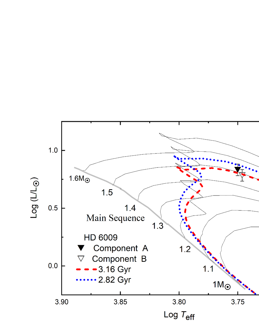
Figure 4: The system’s components on the evolutionary tracks of Girardi et al. (2000).

Table 7: Parameters of the system’s components.

Component	a	b
$T_{\rm eff}$ (K)	$5625\pm 75$	$5575\pm 75$
Radius (R⊙)	$2.75\pm 0.50$	$2.65\pm 0.50$
$\log g$	$3.75\pm 0.25$	$3.75\pm 0.25$
$L(L_{\odot})$	$6.80\pm 0.75$	$6.09\pm 0.75$
$M_{v}$ †	$2\hbox{$.\!\!^{m}$}80\pm 0.30$	$2\hbox{$.\!\!^{m}$}93\pm 0.30$
Mass, ($M_{\odot})$	$1.42\pm 0.15$	$1.40\pm 0.15$
$\overline{\rho}(\overline{\rho}_{\odot})$	$0.07\pm 0.02$	$0.10\pm 0.02$
Sp. Type‡	G6	G6
luminosity class	IV	IV
Age (Gy)	$3.1\pm 0.5$

^†depending on the individual synthetic spectra (Table  6).
^‡depending on the tables of Gray (2005).

Table 8: Comparison between the observational and synthetic entire magnitudes, colours and magnitude differences of the system.

	$\textrm{Obs}.^{*}$	Synth. (this work)
$V_{J}$	$6\hbox{$.\!\!^{m}$}71$	$6\hbox{$.\!\!^{m}$}71\pm 0.03$
$B_{T}$	$7\hbox{$.\!\!^{m}$}683\pm 0.008$	$7\hbox{$.\!\!^{m}$}64\pm 0.03$
$V_{T}$	$6\hbox{$.\!\!^{m}$}806\pm 0.006$	$6\hbox{$.\!\!^{m}$}79\pm 0.03$
$(B-V)_{J}$	$0\hbox{$.\!\!^{m}$}783\pm 0.007$	$0\hbox{$.\!\!^{m}$}84\pm 0.04$
$\triangle m$	$0\hbox{$.\!\!^{m}$}18^{\dagger}$	$0\hbox{$.\!\!^{m}$}18\pm 0.04$
∗See Table 2.
†See section  III.1 .

VI Conclusions

On the basis of analyzing the binary system HD6009 using the method of atmospheric modeling and dynamical analysis for studying VCBSs, the following main conclusions can be drawn:

1. The complete set of the physical and geometrical parameters of the system’s components were estimated depending on the best fit between the observational SED and synthetic ones built using the atmospheric modeling of the individual components.

2. A modification to the parallax of the system is introduced within the error of Hipparcos parallax measurement.

3. The estimated parameters show a good consistency with the previously published ones.

4. Depending on the parameters of the system’s components and their positions on the evolutionary tracks, we showed that the system consists of a twin G6 and G5 subgiant stars.

5. The entire and individual $UBVR$ Johnson-Cousins, $uvby$ Strömgren and $BV$ Tycho synthetic magnitudes and colors of the system were calculated.

6. Finally, the fragmentation was proposed as the most likely process for the formation and evolution of the system.

References

- Al-Wardat (2012) Al-Wardat, M. 2012, Publications of the Astronomical Society of Australia, 29, 523
- Al-Wardat (2002a) Al-Wardat, M. A. 2002a, Bull. Special Astrophys. Obs., 53, 51
- Al-Wardat (2002b) Al-Wardat, M. A. 2002b, Bull. Special Astrophys. Obs., 53, 58
- Al-Wardat (2007) Al-Wardat, M. A. 2007, Astronomische Nachrichten, 328, 63
- Al-Wardat (2008) Al-Wardat, M. A. 2008, Astrophysical Bulletin, 63, 361
- Al-Wardat (2009) Al-Wardat, M. A. 2009, Astronomische Nachrichten, 330, 385
- Al-Wardat et al. (2013a) Al-Wardat, M. A., Balega, Y. Y., Leushion, V. V., et al. 2013a, arXiv:1311.5737
- Al-Wardat & Widyan (2009) Al-Wardat, M. A., & Widyan, H. 2009, Astrophysical Bulletin, 64, 365
- Al-Wardat et al. (2013b) Al-Wardat, M. A., Widyan, H. S., & Al-thyabat, A. 2013b, arXiv:1311.5721
- Balega et al. (2004) Balega, I., Balega, Y. Y., Maksimov, A. F., et al. 2004, Astronom. and Astrophys., 422, 627
- Balega et al. (2006a) Balega, I. I., Balega, A. F., Maksimov, E. V., et al. 2006a, Bull. Special Astrophys. Obs., 59, 20
- Balega et al. (2002) Balega, I. I., Balega, Y. Y., Hofmann, K.-H., et al. 2002, Astronom. and Astrophys., 385, 87
- Balega et al. (2006b) Balega, I. I., Balega, Y. Y., Hofmann, K.-H., et al. 2006b, Astronom. and Astrophys., 448, 703
- Balega et al. (2007) Balega, I. I., Balega, Y. Y., Maksimov, A. F., et al. 2007, Astrophysical Bulletin, 62, 339
- Bonnell (1994) Bonnell, I. A. 1994, Monthly Notices Roy. Astronom. Soc., 269, 837
- ESA (1997) ESA. 1997, The Hipparcos and Tycho Catalogues (ESA)
- Girardi et al. (2000) Girardi, L., Bressan, A., Bertelli, G., & Chiosi, C. 2000, Astronom. and Astrophys. Suppl. Ser., 141, 371
- Gray (2005) Gray, D. F. 2005, The Observation and Analysis of Stellar Photospheres, ed. Gray, D. F.
- Horch et al. (2012) Horch, E. P., Bahi, L. A. P., Gaulin, J. R., et al. 2012, Astronom. J., 143, 10
- Horch et al. (2010) Horch, E. P., Falta, D., Anderson, L. M., et al. 2010, Astronom. J., 139, 205
- Horch et al. (2011) Horch, E. P., Gomez, S. C., Sherry, W. H., et al. 2011, Astronom. J., 141, 45
- Horch et al. (2004) Horch, E. P., Meyer, R. D., & van Altena, W. F. 2004, Astronom. J., 127, 1727
- Horch et al. (2002) Horch, E. P., Robinson, S. E., Meyer, R. D., et al. 2002, Astronom. J., 123, 3442
- Horch et al. (2008) Horch, E. P., van Altena, W. F., Cyr, Jr., W. M., et al. 2008, Astronom. J., 136, 312
- Lang (1992) Lang, K. R. 1992, Astrophysical Data I. Planets and Stars., ed. K. R. Lang
- Maíz Apellániz (2006) Maíz Apellániz, J. 2006, Astronom. J., 131, 1184
- Maíz Apellániz (2007) Maíz Apellániz, J. 2007, in Astronomical Society of the Pacific Conference Series, Vol. 364, The Future of Photometric, Spectrophotometric and Polarimetric Standardization, ed. C. Sterken, 227
- Mason et al. (2009) Mason, B. D., Hartkopf, W. I., Gies, D. R., Henry, T. J., & Helsel, J. W. 2009, Astronom. J., 137, 3358
- Mason et al. (2001) Mason, B. D., Hartkopf, W. I., Holdenried, E. R., & Rafferty, T. J. 2001, Astronom. J., 121, 3224
- Mason et al. (1999) Mason, B. D., Martin, C., Hartkopf, W. I., et al. 1999, Astronom. J., 117, 1890
- Pluzhnik (2005) Pluzhnik, E. A. 2005, Astronom. and Astrophys., 431, 587
- Schlafly & Finkbeiner (2011) Schlafly, E. F., & Finkbeiner, D. P. 2011, Astrophys. J. , 737, 103
- Yoss (1961) Yoss, K. M. 1961, Astrophys. J. , 134, 809
- Zinnecker & Mathieu (2001) Zinnecker, H., & Mathieu, R., eds. 2001, IAU Symposium, Vol. 200, The Formation of Binary Stars