Sequential anomaly detection
under sampling constraints

Abstract

The problem of sequential anomaly detection is considered, where multiple data sources are monitored in real time and the goal is to identify the “anomalous” ones among them, when it is not possible to sample all sources at all times. A detection scheme in this context requires specifying not only when to stop sampling and which sources to identify as anomalous upon stopping, but also which sources to sample at each time instance until stopping. A novel formulation for this problem is proposed, in which the number of anomalous sources is not necessarily known in advance and the number of sampled sources per time instance is not necessarily fixed. Instead, an arbitrary lower bound and an arbitrary upper bound are assumed on the number of anomalous sources, and the fraction of the expected number of samples over the expected time until stopping is required to not exceed an arbitrary, user-specified level. In addition to this sampling constraint, the probabilities of at least one false alarm and at least one missed detection are controlled below user-specified tolerance levels. A general criterion is established for a policy to achieve the minimum expected time until stopping to a first-order asymptotic approximation as the two familywise error rates go to zero. Moreover, the asymptotic optimality is established of a family of policies that sample each source at each time instance with a probability that depends on past observations only through the current estimate of the subset of anomalous sources. This family includes, in particular, a novel policy that requires minimal computation under any setup of the problem.

I Introduction

In various engineering and scientific areas data are often collected in real time over multiple streams, and it is of interest to quickly identify those data streams, if any, that exhibit outlying behavior. In brain science, for example, it is desirable to identify groups of cells with large vibration frequency, as this is a symptom for the development of a particular malfunctioning [1]. In fraud prevention security systems in e-commerce, it is desirable to identify transition links with low transition rate, as this may be an indication that a link is tapped [2]. Such applications, among many others, motivate the study of sequential multiple testing problems where the data for the various hypotheses are generated by distinct sources, there are two hypotheses for each data source, and the goal is to identify as quickly as possible the “anomalous” sources, i.e., those in which the alternative hypothesis is correct. In certain works, e.g., [3, 4, 5, 6, 7, 8], it is assumed that all sources are sampled at each time instance, whereas in others, e.g., [9, 10, 11, 12, 13, 14, 15, 16, 17], only a fixed number of sources (typically, only one) can be sampled at each time instance. In the latter case, apart from when to stop sampling and which data sources to identify as anomalous upon stopping, one also needs to specify which sources to sample at every time instance until stopping.

The latter problem, which is often called sequential anomaly detection in the literature, can be viewed as a special case of the sequential multi-hypothesis testing problem with controlled sensing (or observation control), where the goal is to solve a sequential multi-hypothesis testing problem while taking at each time instance an action that influences the distribution of the observations [18, 19, 20, 21, 22, 23, 24, 25, 26, 27, 28]. In the anomaly detection case, the action is the selection of the sources to be sampled, whereas the hypotheses correspond to the possible subsets of anomalous sources. Therefore, policies and results in the context of sequential multi-hypothesis testing with controlled sensing are applicable, in principle at least, to the sequential anomaly detection problem. Such a policy was first proposed in [18] in the case of two hypotheses, and subsequently generalized in [20, 21] to the case of an arbitrary, finite number of hypotheses. When applied to the sequential anomaly detection problem, this policy samples each subset of sources of the allowed size at each time instance with a certain probability that depends on the past observations only through the currently estimated subset of anomalous sources.

In general, the implementation of the policy in [20] requires solving, for each subset of anomalous sources, a linear system where the number of equations is equal to the number of sources and the number of unknowns is equal to the number of all subsets of sources of the allowed size. Moreover, its asymptotic optimality has been established only under restrictive assumptions, such as when the following hold simultaneously: it is known a priori that there is only one anomalous source, it is possible to sample only one source at a time, the testing problems are identical, and the sources generate Bernoulli random variables under each hypothesis [21, Appendix A]. To avoid such restrictions, it has been proposed to modify the policy in [20] at an appropriate subsequence of time instances, at which each subset of sources of the allowed size is sampled with the same probability [18, Remark 7],[25]. Such a modified policy was shown in [25] to always be asymptotically optimal, as long as the log-likelihood ratio statistic of each observation has a finite second moment.

A goal of the present work is to show that the unmodified policy in [20] is always asymptotically optimal in the context of the above sequential anomaly detection problem, as long as the log-likelihood ratio statistic of each observation has a finite first moment. However, our main goal in this paper is to propose a more general framework for the problem of sequential anomaly detection with sampling constraints that (i) does not rely on the restrictive assumption that the number of anomalous sources is known in advance, (ii) allows for two distinct error constraints and captures the asymmetry between a false alarm, i.e., falsely identifying a source as anomalous, and a missed detection, i.e., failing to detect an anomalous source, and most importantly, (iii) relaxes the hard sampling constraint that the same number of sources must be sampled at each time instance, and (iv) admits an asymptotically optimal solution that is convenient to implement under any setup of the problem.

To be more specific, in this paper we assume an arbitrary, user-specified lower bound and an arbitrary, user-specified upper bound on the number of anomalous sources. This setup includes the case of no prior information, the case where the number of anomalous sources is known in advance, as well as more realistic cases of prior information, such as when there is only a non-trivial upper bound on the number of anomalous sources. Moreover, we require control of the probabilities of at least one false alarm and at least one missed detection below arbitrary, user-specified levels. Both these features are taken into account in [6] when all sources are observed at all times. Thus, the present paper can be seen as a generalization of [6] to the case that it is not possible to observe all sources at all times. However, instead of demanding that the number of sampled sources per time instance be fixed, as in [9, 10, 11, 14, 12, 13, 15, 16, 17], we only require that the ratio of the expected number of observations over the expected time until stopping not exceed a user-specified level. This leads to a more general formulation for sequential anomaly detection compared to those in [9, 10, 11, 14, 12, 13, 15, 16, 17], which at the same time is not a special case of the sequential multi-hypothesis testing problem with controlled sensing in [18, 19, 20, 21, 22, 23, 24, 25, 26, 27, 28]. Thus, while existing policies in the literature are applicable to the proposed setup, this is not the case for the existing universal lower bounds.

Our first main result on the proposed problem is a criterion for a policy (that employs the stopping and decision rules in [6] and satisfies the sampling constraint) to achieve the optimal expected time until stopping to a first-order asymptotic approximation as the two familywise error probabilities go to 0. Indeed, we show that such a policy is asymptotically optimal in the above sense, if it samples each source with a certain minimum long-run frequency that depends on the source itself and the true subset of anomalous sources. Our second main result is that the latter condition holds, simultaneously for every possible scenario regarding the anomalous sources, by policies that sample each source at each time instance with a probability that is not smaller than the above minimum long-run frequency that corresponds to the current estimate of the subset of anomalous sources. This implies the asymptotic optimality of the unmodified policy in [20], as well as of a much simpler policy according to which the sources are sampled at each time instance conditionally independent of one another given the current estimate of the subset of anomalous sources. Indeed, the implementation of the latter policy, unlike that in [20], involves minimal computational and storage requirements under any setup of the problem. Moreover, we present simulation results that suggest that this computational simplicity does not come at the price of performance deterioration (relative to the policy in [20]).

Finally, to illustrate the gains of asymptotic optimality, we consider the straightforward policy in which the sources are sampled in tandem. We compute its asymptotic relative efficiency and we show that it is asymptotically optimal only in a very special setup of the problem. Moreover, our simulation results suggest that, apart from this special setup, its actual performance loss relative to the above asymptotically optimal rules is (much) larger than the one implied by its asymptotic relative efficiency when the target error probabilities are not (very) small.

The remainder of the paper is organized as follows: in Section II we formulate the proposed problem. In Section III we present a family of policies that satisfy the error constraints, and we introduce an auxiliary consistency property.In Section IV we introduce a family of sampling rules on which we focus in this paper. In Section V we present the asymptotic optimality theory of this work. In Section VI we discuss alternative sampling approaches in the literature, and in Section VII we present the results of our simulation studies. In Section VIII we conclude and discuss potential generalizations, as well as directions for further research. The proofs of all main results are presented in Appendices B, C, D, whereas in Appendix A we state and prove two supporting lemmas.

We end this section with some notations we use throughout the paper. We use $:=$ to indicate the definition of a new quantity and $\equiv$ to indicate a duplication of notation. We set $\mathbb{N}:=\{1,2\ldots,\}$ and $[n]:=\{1,\ldots,n\}$ for $n\in\mathbb{N}$, we denote by $A^{c}$ the complement, by $|A|$ the size and by $2^{A}$ the powerset of a set $A$, by $\lfloor a\rfloor$ the floor and by $\lceil a\rceil$ the ceiling of a positive number $a$, and by $\mathbf{1}$ the indicator of an event. We write $x\sim y$ when $\lim(x/y)=1$, $x\gtrsim y$ when $\liminf(x/y)\geq 1$, and $x\lesssim y$ when $\limsup(x/y)\leq 1$, where the limit is taken in some sense that will be specified. Moreover, iid stands for independent and identically distributed, and we say that a sequence of positive numbers $(a_{n})$ is summable if $\sum_{n=1}^{\infty}a_{n}<\infty$ and exponentially decaying if there are real numbers $c,d>0$ such that $a_{n}\leq c\exp\{-d\,n\}$ for every $n\in\mathbb{N}$. A property that we use in our proofs is that if $(a_{n})$ is exponentially decaying, so is the sequence $(\sum_{m\geq\zeta n}a_{m})$, for any $\zeta\in(0,1]$.

II Problem formulation

Let $(\mathbb{S},\mathcal{S})$ be an arbitrary measurable space and let $(\Omega,\mathcal{F},\mathsf{P})$ be a probability space that hosts $M$ independent sequences of iid $\mathbb{S}$-valued random elements, $\{X_{i}(n):n\in\mathbb{N}\},i\in[M]$, which are generated by $M$ distinct data sources, as well as an independent sequence of iid random vectors, $\{Z(n):n=0,1,\ldots\}$, to be used for randomization purposes. Specifically, each $Z(n):=(Z_{0}(n),Z_{1}(n),\ldots,Z_{M}(n))$ is a vector of independent random variables, uniform in $(0,1)$, and each $X_{i}(n)$ has density $f_{i}$, with respect to some $\sigma$-finite measure $\nu_{i}$, that is equal to either $f_{1i}$ or $f_{0i}$. For every $i\in[M]$ we say that source $i$ is “anomalous” if $f_{i}=f_{1i}$ and we assume that the Kullback-Leibler divergences of $f_{1i}$ and $f_{0i}$ are positive and finite, i.e.,

$$\begin{split}I_{i}&:=\int_{\mathbb{S}}\log(f_{1i}/f_{0i})\,f_{1i}\,d\nu_{i}\in(0,\infty),\\ J_{i}&:=\int_{\mathbb{S}}\log(f_{0i}/f_{1i})\,f_{0i}\,d\nu_{i}\in(0,\infty).\end{split}$$ (1)

We assume that it is known a priori that there are at least $\ell$ and at most $u$ anomalous sources, where $\ell$ and $u$ are given, user-specified integers such that $0\leq\ell\leq u\leq M$, with the understanding that if $\ell=u$, then $0<\ell<M$. Thus, the family of all possible subsets of anomalous sources is $\mathcal{P}_{\ell,u}:=\{A\subseteq[M]:\ell\leq|A|\leq u\}$. In what follows, we denote by $\mathsf{P}_{A}$ the underlying probability measure and by $\mathsf{E}_{A}$ the corresponding expectation when the subset of anomalous sources is $A\in\mathcal{P}_{\ell,u}$, and we simply write $\mathsf{P}$ and $\mathsf{E}$ whenever the identity of the subset of anomalous sources is not relevant.

The problem we consider in this work is the identification of the anomalous sources, if any, on the basis of sequentially acquired observations from all sources, when however it is not possible to observe all of them at every sampling instance. Specifically, we have to specify a random time $T$, at which sampling is terminated, and two random sequences, $R:=\{R(n),n\geq 1\}$ and $\Delta:=\{\Delta(n),n\in\mathbb{N}\}$, so that $R(n)\subseteq[M]$ represents the subset of sources that are sampled at time $n$ when $n\leq T$, and $\Delta(n)\equiv\Delta_{n}\in\mathcal{P}_{\ell,u}$ represents the subset of sources that are identified as anomalous when $T=n$. The decisions whether to stop or not at each time instance, which sources to sample next in the latter case, and which ones to identify as anomalous in the former, must be based on the already available information. Thus, we say that $R$ is a sampling rule if $R(n)$ is $\mathcal{F}_{n-1}^{R}$–measurable for every $n\in\mathbb{N}$, where

$$\begin{split}\mathcal{F}_{n}^{R}&:=\sigma\left(\mathcal{F}_{n-1}^{R},\,Z(n),\,\{X_{i}(n):i\in R(n)\}\right),\quad n\in\mathbb{N},\\ \mathcal{F}_{0}^{R}&:=\sigma(Z(0)).\end{split}$$ (2)

Moreover, we say that the triplet $(R,T,\Delta)$ is a policy if $R$ is a sampling rule, $\{T=n\}\in\mathcal{F}^{R}_{n}$ and $\Delta_{n}$ is $\mathcal{F}^{R}_{n}-$measurable for every $n\in\mathbb{N}$, in which case we refer to $T$ as a stopping rule and to $\Delta$ as a decision rule. For any sampling rule $R$, we denote by $R_{i}(n)$ the indicator of whether source $i$ is sampled at time $n$, i.e., $R_{i}(n):=\mathbf{1}\{i\in R(n)\}$, and by $N_{i}^{R}(n)$ (resp. $\pi_{i}^{R}(n)$) the number (resp. proportion) of times source $i$ is sampled in the first $n$ time instances, i.e.,

$$N^{R}_{i}(n) :=\sum_{m=1}^{n}R_{i}(m),\quad\ \pi_{i}^{R}(n):=N^{R}_{i}(n)/n.$$

We say that a policy $(R,T,\Delta)$ belongs to class $\mathcal{C}(\alpha,\beta,\ell,u,K)$ if its probabilities of at least one false alarm and at least one missed detection upon stopping do not exceed $\alpha$ and $\beta$ respectively, i.e.,

$$\begin{split}\mathsf{P}_{A}\left(T<\infty,\,\Delta_{T}\setminus A\neq\emptyset\right)\leq\alpha\quad\forall\,A\in\mathcal{P}_{\ell,u},\\ \mathsf{P}_{A}\left(T<\infty,\,A\setminus\Delta_{T}\neq\emptyset\right)\leq\beta\quad\forall\,A\in\mathcal{P}_{\ell,u},\end{split}$$ (3)

where $\alpha,\beta$ are user-specified numbers in $(0,1)$, and the ratio of its expected total number of observations over its expected time until stopping does not exceed $K$, i.e.,

$$\sum_{i=1}^{M}\mathsf{E}\left[N_{i}^{R}(T)\right]\leq K\;\mathsf{E}[T],$$ (4)

where $K$ is a user-specified, real number in $(0,M]$. Note that, in view of the identity

$$\sum_{i=1}^{M}\mathsf{E}\left[N_{i}^{R}(T)\right] =\mathsf{E}\left[\sum_{n=1}^{T}\mathsf{E}\left[|R(n)|\;|\;\mathcal{F}_{n-1}^{R}\right]\right],$$

constraint (4) is clearly satisfied when

$$\sup_{n\leq T}\,\mathsf{E}\left[|R(n)|\;|\;\mathcal{F}_{n-1}^{R}\right]\leq K,$$ (5)

This is the case, for example, when at most $\lfloor K\rfloor$ sources are sampled at each time instance up to stopping, i.e., when $|R(n)|\leq\lfloor K\rfloor$ for every $n\leq T$.

Our main goal in this work is, for any given $\ell,u,K$, to obtain policies that attain the smallest possible expected time until stopping,

$$\mathcal{J}_{A}(\alpha,\beta,\ell,u,K):=\inf_{(R,T,\Delta)\in\mathcal{C}(\alpha,\beta,\ell,u,K)}\;\mathsf{E}_{A}[T],$$ (6)

simultaneously under every $A\in\mathcal{P}_{\ell,u}$, to a first-order asymptotic approximation as $\alpha$ and $\beta$ go to 0. Specifically, when $\ell=u$, we allow $\alpha$ and $\beta$ to go to 0 at arbitrary rates, but when $\ell<u$, we assume that

$$\exists\;r\in(0,\infty):|\log\alpha|\sim r\,|\log\beta|.$$ (7)

III A family of policies

In this section we introduce the statistics that we use in this work, a family of policies that satisfy the error constraint (3), as well as an auxiliary consistency property.

III-A Log-likelihood ratio statistics

Let $A,C\in\mathcal{P}_{\ell,u}$ and $n\in\mathbb{N}$. We denote by $\Lambda^{R}_{A,C}(n)$ the log-likelihood ratio of $\mathsf{P}_{A}$ versus $\mathsf{P}_{C}$ based on the first $n$ time instances when the sampling rule is $R$, i.e.,

$$\Lambda^{R}_{A,C}(n):=\log\frac{d\mathsf{P}_{A}}{d\mathsf{P}_{{C}}}\left(\mathcal{F}^{R}_{n}\right),$$ (8)

and we observe that it admits the following recursion:

$$\Lambda^{R}_{A,C}(n) =\Lambda^{R}_{A,C}(n-1)+\sum_{i\in A\setminus{C}}g_{i}(X_{i}(n))\,R_{i}(n)-\sum_{j\in{C}\setminus A}g_{j}(X_{j}(n))\,R_{j}(n),$$ (9)

where $\Lambda^{R}_{A,C}(0):=0$ and $g_{i}:=\log\left(f_{1i}/f_{0i}\right),\,i\in[M]$. Indeed, this follows by $\eqref{filtration}$ and the fact that $R(n)$ is $\mathcal{F}_{n-1}^{R}$-measurable, $X_{i}(n)$ is independent of $\mathcal{F}_{n-1}^{R}$ and its density under $\mathsf{P}_{A}$ is $f_{1i}$ if $i\in A$ and $f_{0i}$ if $i\notin A$, and $Z(n)$ is independent of both $\mathcal{F}_{n-1}^{R}$ and $\{X_{i}(n):i\in[M]\}$ and has the same density under $\mathsf{P}_{A}$ and $\mathsf{P}_{C}$.

For any $i,j\in[M]$ we write

$$\Lambda^{R}_{A,C}(n) \equiv\Lambda^{R}_{ij}(n)\quad\text{when }\quad A=\{i\},C=\{j\},$$

$$\Lambda^{R}_{A,C}(n) \equiv\Lambda^{R}_{i}(n)\quad\text{when }\quad A=\{i\},C=\emptyset,$$

and we observe that the above recursion implies that

$$\Lambda^{R}_{i}(n) =\sum_{m=1}^{n}g_{i}(X_{i}(m))\,R_{i}(m),$$ (10)

$$\Lambda^{R}_{A,C}(n) =\sum_{i\in A\setminus{C}}\Lambda^{R}_{i}(n)-\sum_{j\in{C}\setminus A}\Lambda^{R}_{j}(n).$$ (11)

In particular, for any $i,j\in[M]$ we have

$$\Lambda^{R}_{ij}(n)=\Lambda^{R}_{i}(n)-\Lambda^{R}_{j}(n).$$

In what follows, we refer to $\Lambda^{R}_{i}(n)$ as the local log-likelihood ratio (LLR) of source $i$ at time $n$. We introduce the order statistics of the LLRs at time $n$,

$$\Lambda^{R}_{(1)}(n)\geq\ldots\geq\Lambda^{R}_{(M)}(n),$$

and we denote by $w^{R}_{i}(n),i\in[M]$ the corresponding indices, i.e.,

$$\Lambda^{R}_{(i)}(n):=\Lambda^{R}_{w^{R}_{i}(n)}(n),\quad i\in[M].$$

Moreover, we denote by $p^{R}(n)$ the number of positive LLRs at time $n$, i.e.,

$$p^{R}(n)\ :=\sum_{i=1}^{M}\mathbf{1}\{\Lambda^{R}_{i}(n)>0\},$$

and we also set

$$\Lambda^{R}_{(0)}(n):=+\infty,\qquad\Lambda^{R}_{(M+1)}(n):=-\infty.$$

III-B Stopping and decision rules

We next show that for any sampling rule $R$ there is a stopping rule, which we will denote by $T^{R}$, and a decision rule, which we will denote by $\Delta^{R}$, such that the policy $(R,T^{R},\Delta^{R})$ satisfies the error constraint (3). Their forms depend on whether the number of anomalous sources is known in advance or not, i.e., on whether $\ell=u$ or $\ell<u$. Specifically, when $\ell=u$, we stop as soon as the $\ell^{th}$ largest LLR exceeds the next one by $c>0$, i.e.,

$$T^{R} :=\inf\left\{n\in\mathbb{N}:\;\Lambda^{R}_{(\ell)}(n)-\Lambda^{R}_{(\ell+1)}(n)\geq c\right\},$$ (12)

and we identify as anomalous the sources with the $\ell$ largest LLRs, i.e.,

$$\Delta^{R}_{n} :=\left\{w^{R}_{1}(n),\ldots,w^{R}_{\ell}(n)\right\},\quad n\in\mathbb{N}.$$ (13)

When the number of anomalous sources is completely unknown ($\ell=0$ and $u=M$), we stop as soon as the value of every LLR is outside $(-a,b)$ for some $a,b>0$, i.e.,

$$T^{R} :=\inf\left\{n\in\mathbb{N}:\;\Lambda^{R}_{i}(n)\notin(-a,b)\quad\text{for all}\quad i\in[M]\right\},$$ (14)

and we identify as anomalous the sources with positive LLRs, i.e.,

$$\Delta^{R}_{n} :=\left\{i\in[M]:\;\Lambda^{R}_{i}(n)>0\right\},\quad n\in\mathbb{N}.$$ (15)

When $\ell<u$, in general, we combine the stopping rules of the two previous cases and we set

$$\begin{split}T^{R}:=\inf\{n\in\mathbb{N}:\quad&\text{either}\quad\Lambda^{R}_{(\ell+1)}(n){\leq}-a\quad\&\quad\Lambda^{R}_{(\ell)}(n)-\Lambda^{R}_{(\ell+1)}(n)\geq c,\\ \quad&\;\text{or}\quad\quad\ell\leq p^{R}(n)\leq u\qquad\&\qquad\Lambda^{R}_{i}(n)\notin(-a,b)\quad\forall\;i\in[M],\\ \quad&\;\text{or}\quad\quad\;\Lambda^{R}_{(u)}(n)\geq b\qquad\&\quad\Lambda^{R}_{(u)}(n)-\Lambda^{R}_{(u+1)}(n)\geq d\},\end{split}$$ (16)

where $a,b,c,d>0$, and we use the following decision rule:

$$\Delta^{R}_{n} :=\left\{w^{R}_{i}(n):\;i=1,\ldots,(p^{R}(n)\vee\ell)\wedge u\right\},\quad n\in\mathbb{N}.$$ (17)

That is, we identify as anomalous the sources with positive LLRs as long as their number is between $\ell$ and $u$. If this number is larger than $u$ (resp. smaller than $\ell$), then we declare as anomalous the sources with the $u$ (resp. $\ell$) largest LLRs.

Proposition III.1

Let $R$ be an arbitrary sampling rule.

• When $\ell=u$, $(R,T^{R},\Delta^{R})$ satisfies the error constraint (3) if

  $$c=|\log(\alpha\wedge\beta)|+\log(\ell(M-\ell)).$$ (18)

• When $\ell<u$, $(R,T^{R},\Delta^{R})$ satisfies the error constraint (3) if

  $$\begin{split}a&=|\log\beta|+\log M,\quad c=|\log\alpha|+\log((M-\ell)M),\\ b&=|\log\alpha|+\log M,\quad d=|\log\beta|+\log(uM).\end{split}$$ (19)

Proof:

When all sources are sampled at all times, this is shown in [6, Theorems 3.1, 3.2]. The same proof applies when $K<M$ for any sampling rule $R$.
∎

In view of the above result, in what follows we assume that the thresholds in $T^{R}$ are selected according to (18) when $\ell=u$ and according to (19) when $\ell<u$. While this is a rather conservative choice, it will be sufficient for obtaining asymptotically optimal policies. For this reason, in what follows we say that a sampling rule, $R$, that satisfies the sampling constraint (4) with $T=T^{R}$, is asymptotically optimal under $\mathsf{P}_{A}$, for some $A\in\mathcal{P}_{\ell,u}$, if

$$\mathsf{E}_{A}\left[T^{R}\right]\sim\mathcal{J}_{A}(\alpha,\beta,\ell,u,K)$$

as $\alpha$ and $\beta$ go to $0$ at arbitrary rates when $\ell=u$ and so that (7) holds when $\ell<u$. We simply say that $R$ is asymptotically optimal if it is asymptotically optimal under $\mathsf{P}_{A}$ for every $A\in\mathcal{P}_{\ell,u}$. We next introduce a weaker property, which will be useful for establishing asymptotic optimality.

III-C Exponential consistency

For any sampling rule $R$ and any subset $A\in\mathcal{P}_{\ell,u}$ we denote by $\sigma_{A}^{R}$ the random time starting from which the sources in $A$ are the ones estimated as anomalous by $\Delta^{R}$, i.e.,

$$\sigma^{R}_{A}:=\inf\left\{n\in\mathbb{N}:\Delta^{R}_{m}=A\quad\text{for all}\;\;m\geq n\right\},$$ (20)

and we say that $R$ is exponentially consistent under $\mathsf{P}_{A}$ if $\mathsf{P}_{A}(\sigma_{A}^{R}>n)$ is an exponentially decaying sequence. We simply say that $R$ is exponentially consistent if it is exponentially consistent under $\mathsf{P}_{A}$ for every $A\in\mathcal{P}_{\ell,u}$. The following theorem states sufficient conditions for exponential consistency under $\mathsf{P}_{A}$.

Theorem III.1

Let $A\in\mathcal{P}_{\ell,u}$ and let $R$ be an arbitrary sampling rule.

• When $\ell<u$, $R$ is exponentially consistent under $\mathsf{P}_{A}$ if there exists a $\rho>0$ such that $\mathsf{P}_{A}\left(\pi^{R}_{i}(n)<\rho\right)$ is exponentially decaying for every $i\in A$ if $|A|>\ell$ and for every $i\notin A$ if $|A|<u$.

• When $\ell=u$, $R$ is exponentially consistent under $\mathsf{P}_{A}$ if there exists a $\rho>0$ such that $\mathsf{P}_{A}\left(\pi^{R}_{i}(n)<\rho\right)$ is exponentially decaying either for every $i\in A$ or for every $i\notin A$.

Proof:

Appendix B.
∎

Remark: Theorem III.1 reveals that when $|A|=\ell>0$ or $|A|=u<M$, it is possible to have exponentially consistency under $\mathsf{P}_{A}$ without sampling at all certain sources. Specifically, when $|A|=\ell<u$ (resp. $|A|=u>\ell$) it is not necessary to sample any source in $A$ (resp. $A^{c}$). On the other hand, when $|A|=\ell=u$, it suffices to sample either all sources in $A$ or all of them in $A^{c}$.

IV Probabilistic sampling rules

In this section we introduce a family of sampling rules and we show how to design them in order to satisfy the sampling constraint (5) and in order to be exponentially consistent. Thus, we say that a sampling rule $R$ is probabilistic if there exists a function $q^{R}:2^{[M]}\times\mathcal{P}_{\ell,u}\to[0,1]$ such that for every $n\in\mathbb{N}$, $D\in\mathcal{P}_{\ell,u}$, and $B\subseteq[M]$ we have

$$q^{R}\left(B;D\right):=\mathsf{P}\left(R(n+1)=B\,|\,\mathcal{F}^{R}_{n},\Delta^{R}_{n}=D\right),$$ (21)

i.e., $q^{R}\left(B;D\right)$ is the probability that $B$ is the subset of sampled sources when $D$ is the currently estimated subset of anomalous sources. If $R$ is a probabilistic sampling rule, then for every $i\in[M]$ and $D\in\mathcal{P}_{\ell,u}$ we set

$$\begin{split}c^{R}_{i}\left(D\right)&:=\mathsf{P}\left(R_{i}(n+1)=1\,|\,\mathcal{F}^{R}_{n},\Delta^{R}_{n}=D\right)\\ &=\sum_{B\subseteq[M]:\,i\in B}q^{R}\left(B;D\right),\end{split}$$ (22)

i.e., $c^{R}_{i}(D)$ is the probability that source $i$ is sampled when $D$ is the currently estimated subset of anomalous sources.

We refer to a probabilistic sampling rule $R$ as Bernoulli if for every $D\in\mathcal{P}_{\ell,u}$ and $B\subseteq[M]$ we have

$$q^{R}(B;D)=\prod_{i\in B}c^{R}_{i}(D)\prod_{j\notin B}\left(1-c^{R}_{j}(D)\right),$$ (23)

i.e., if the sources are sampled at each time instance conditionally independent of one another given the currently estimated subset of anomalous sources. Indeed, such a sampling rule admits a representation of the form

$$R_{i}(n+1) =\mathbf{1}\left\{Z_{i}(n)\leq c^{R}_{i}\left(\Delta_{n}^{R}\right)\right\},\quad i\in[M],n\in\mathbb{N},$$ (24)

where $Z_{1}(n),\ldots,Z_{M}(n)$ are iid and uniform in $(0,1)$, thus, its implementation at each time instance requires the realization of $M$ Bernoulli random variables.

The following proposition provides a sufficient condition for a probabilistic sampling rule to satisfy the sampling constraint (5), and consequently (4), for any $\{\mathcal{F}_{n}^{R}\}$-stopping time $T$.

Proposition IV.1

If $R$ is a probabilistic sampling rule such that

$$\sum_{i=1}^{M} c^{R}_{i}(D)\leq K\quad\text{for every }\;D\in\mathcal{P}_{\ell,u},$$ (25)

then (5) holds for any $\{\mathcal{F}_{n}^{R}\}$-stopping time $T$.

Proof:

For any $n\in\mathbb{N}$ and any probabilistic sampling rule $R$ we have

$$\mathsf{E}\left[|R(n)|\;|\;\mathcal{F}_{n-1}^{R}\right]=\sum_{i=1}^{M}\mathsf{P}\left(R_{i}(n)=1\;|\;\mathcal{F}_{n-1}^{R}\right)=\sum_{i=1}^{M}c^{R}_{i}(\Delta_{n}^{R}).$$

As a result, if (25) is satisfied, then (5) holds for any $\{\mathcal{F}_{n}^{R}\}$-stopping time, $T$.
∎

Finally, we establish sufficient conditions for the exponentially consistency of a probabilistic sampling rule.

Theorem IV.1

Let $R$ be a probabilistic sampling rule.

• When $\ell<u$, $R$ is exponentially consistent if, for every $D\in\mathcal{P}_{\ell,u}$, $c_{i}^{R}(D)$ is positive for every $i\in D$ if $|D|>\ell$ and every $i\notin D$ if $|D|<u$.

• When $\ell=u$, $R$ is exponentially consistent if, for every $D\in\mathcal{P}_{\ell,u}$, $c_{i}^{R}(D)$ is positive either for every $i\in D$ or for every $i\notin D$.

Proof:

The proof consists in showing that the sufficient conditions of Theorem III.1 are satisfied for every $A\in\mathcal{P}_{\ell,u}$, and is presented in Appendix B.
∎

Remark: Theorem IV.1 implies that when $\ell<u$, a probabilistic sampling rule is exponentially consistent if, whenever the number of estimated anomalous sources is larger than $\ell$ (resp. smaller than $u$), it samples with positive probability any source that is currently estimated as anomalous (resp. non-anomalous). When $\ell=u$, on the other hand, it suffices to sample with positive probability at any time instance either every source that is currently estimated as anomalous or every source that is currently estimated as non-anomalous.

Remark: Unlike the proof of Proposition IV.1, the proof of Theorem IV.1 is quite challenging and it is one of the main contributions of this work from a technical point of view. It relies on two Lemmas, B.1 and B.2, which we state in Appendix B. The proof becomes much easier if we strengthen the assumption of the theorem and assume that every source be sampled with positive probability at every time instance, i.e., if we assumed that $c_{i}^{R}(D)>0$ for every $D\in\mathcal{P}_{\ell,u}$. Indeed, in this case Lemma B.2 becomes redundant, the proof simplifies considerably, and it essentially relies on ideas developed in [18]. However, such an assumption would limit considerably the scope of the asymptotic optimality theory we develop in the next section.

V Asymptotic optimality

In this section we present the asymptotic optimality theory of this work and discuss some of its implications. For this, we first need to introduce some additional notation.

V-A Notation

For $A\subseteq[M]$ with $A\neq\emptyset$ we set

$$I^{*}_{A} :=\min\limits_{i\in A}I_{i},\quad I_{A}:=\frac{|A|}{\sum_{i\in A}(1/I_{i})},\quad\hat{K}_{A}:=|A|\;\frac{I^{*}_{A}}{I_{A}},$$ (26)

and for $A\subseteq[M]$ with $A\neq[M]$ we set

$$J^{*}_{A}:=\min\limits_{i\notin A}J_{i}\quad J_{A}:=\frac{|A^{c}|}{\sum_{i\notin A}(1/J_{i})},\quad\check{K}_{A}:=|A^{c}|\;\frac{J^{*}_{A}}{J_{A}}.$$ (27)

That is, $I^{*}_{A}$ is the minimum and $I_{A}$ the harmonic mean of the Kullback-Leibler information numbers in $\{I_{i}:i\in A\}$, whereas $J^{*}_{A}$ is the minimum and $J_{A}$ the harmonic mean of the Kullback-Leibler information numbers in $\{J_{i}:i\notin A\}$. Moreover, $\hat{K}_{A}$ (resp. $\check{K}_{A}$) is a positive real number smaller or equal to the size of $A$ (resp. $A^{c}$), with the equality attained when $I_{i}=I$ (resp. $J_{i}=J$) for every $i$ in $A$ (resp. $A^{c}$).

Moreover, for $A\subseteq[M]$ with $0<|A|<M$ we set

$$\theta_{A} :=\;I^{*}_{A}/J^{*}_{A},$$ (28)

thus, $\theta_{A}$ is a positive real number that is equal to 1 when $I_{i}=J_{i}$ for every $i\in[M]$.

In Theorem V.1 we also introduce for each $A\in\mathcal{P}_{\ell,u}$ two quantities,

$$x_{A}(r,\ell,u,K)\quad\text{and}\quad y_{A}(r,\ell,u,K),$$ (29)

which will play an important role in the formulation of all results in this section. Although their values depend on $r,\ell,u,K$, in order to lighten the notation we simply write $x_{A}$ and $y_{A}$ unless we want to emphasize their dependence on one or more of these parameters.

V-B A universal asymptotic lower bound

Theorem V.1

Let $A\in\mathcal{P}_{\ell,u}$.

(i) Suppose that $\ell=u$. Then, as $\alpha,\beta\to 0$ we have

$$\mathcal{J}_{A}(\alpha,\beta,\ell,u,K) \gtrsim\frac{|\log(\alpha\wedge\beta)|}{x_{A}\,I^{*}_{A}+y_{A}\,J^{*}_{A}},$$ (30)

where if $\hat{K}_{A}\leq\theta_{A}\check{K}_{A}$,

$$\begin{split}x_{A}&:=(K/\hat{K}_{A})\wedge 1\\ y_{A}&:=\bigl{(}(K-\hat{K}_{A})^{+}/\check{K}_{A}\bigr{)}\wedge 1,\end{split}$$ (31)

and if $\hat{K}_{A}>\theta_{A}\check{K}_{A}$,

$$\begin{split}x_{A}&:=\bigl{(}(K-\check{K}_{A})^{+}/\hat{K}_{A}\bigr{)}\wedge 1\\ y_{A}&:=(K/\check{K}_{A})\wedge 1.\end{split}$$ (32)

(ii) Suppose that $\ell<u$ and let $\alpha,\beta\to 0$ so that (7) holds.

• If $\ell<|A|<u$, then

  $$\begin{split}\mathcal{J}_{A}(\alpha,\beta,\ell,u,K)&\gtrsim\frac{|\log\alpha|}{x_{A}\,I_{A}^{*}}\sim\frac{|\log\beta|}{y_{A}\,J_{A}^{*}},\\ \text{where}\qquad x_{A}&:=\frac{K}{\hat{K}_{A}+(\theta_{A}/r)\check{K}_{A}}\wedge(r/\theta_{A})\wedge 1\\ y_{A}&:=\frac{K}{\check{K}_{A}+(r/\theta_{A})\hat{K}_{A}}\wedge(\theta_{A}/r)\wedge 1.\end{split}$$ (33)

• If $|A|=\ell$, we distinguish two cases:

  • If either $\ell=0$ or $r\leq 1$, then

    $$\begin{split}\mathcal{J}_{A}(\alpha,\beta,\ell,u,K)&\gtrsim\frac{|\log\beta|}{x_{A}\,I_{A}^{*}+y_{A}\,J_{A}^{*}},\quad\\ \text{where}\qquad x_{A}&:=0\\ y_{A}&:=(K/\check{K}_{A})\wedge 1.\end{split}$$ (34)

    If $\ell>0$ and $r>1$, we set $z_{A}:=\theta_{A}/(r-1)$ and we distinguish two further cases:

    • If either $z_{A}\geq 1$ or $K\leq\hat{K}_{A}+z_{A}\,\check{K}_{A}$, then

      $$\begin{split}\mathcal{J}_{A}(\alpha,\beta,\ell,u,K)&\gtrsim\frac{|\log\beta|}{y_{A}\,J_{A}^{*}}\sim\frac{|\log\alpha|}{x_{A}\,I_{A}^{*}+y_{A}\,J_{A}^{*}},\\ \text{where}\qquad x_{A}&:=\frac{K}{\hat{K}_{A}+z_{A}\,\check{K}_{A}}\wedge(1/z_{A})\wedge 1\\ y_{A}&:=\frac{K}{\check{K}_{A}+(1/z_{A})\,\hat{K}_{A}}\wedge z_{A}\wedge 1.\end{split}$$ (35)

    • If   $z_{A}<1$ and $K>\hat{K}_{A}+z_{A}\,\check{K}_{A}$, then

      $$\begin{split}\mathcal{J}_{A}(\alpha,\beta,\ell,u,K)&\gtrsim\frac{|\log\alpha|}{x_{A}\,I^{*}_{A}+y_{A}\,J^{*}_{A}}\\ \;\;\text{where}\qquad x_{A}&:=1\\ y_{A}&:=\bigl{(}(K-\hat{K}_{A})/\check{K}_{A}\bigr{)}\wedge 1.\end{split}$$ (36)

• If $|A|=u$, then we distinguish again two cases:

  • If either $u=M$ or $r\geq 1$, then

    $$\begin{split}\mathcal{J}_{A}(\alpha,\beta,\ell,u,K)&\gtrsim\frac{|\log\alpha|}{x_{A}\,I_{A}^{*}+y_{A}\,J_{A}^{*}}\\ \text{where}\qquad y_{A}&:=0\\ x_{A}&:=(K/\hat{K}_{A})\wedge 1.\end{split}$$ (37)

    If $u<M$ and $r<1$, we set $w_{A}:=(1/\theta_{A})/(1/r-1)$ and we distinguish two further cases:

    • If either $w_{A}\geq 1$ or $K\leq\check{K}_{A}+w_{A}\hat{K}_{A}$, then

      $$\begin{split}\mathcal{J}_{A}(\alpha,\beta,\ell,u,K)&\gtrsim\frac{|\log\alpha|}{x_{A}\,I_{A}^{*}}\sim\frac{|\log\beta|}{x_{A}\,I_{A}^{*}+y_{A}\,J_{A}^{*}},\\ \text{where}\qquad y_{A}&:=\frac{K}{\check{K}_{A}+w_{A}\hat{K}_{A}}\wedge(1/w_{A})\wedge 1\\ x_{A}&:=\frac{K}{\hat{K}_{A}+(1/w_{A})\check{K}_{A}}\wedge w_{A}\wedge 1.\end{split}$$ (38)

    • If $w_{A}<1$ and $K>\check{K}_{A}+w_{A}\hat{K}_{A}$, then

      $$\begin{split}\mathcal{J}_{A}(\alpha,\beta,\ell,u,K)&\gtrsim\frac{|\log\beta|}{x_{A}\,I_{A}^{*}+y_{A}\,J_{A}^{*}},\\ \text{where}\qquad y_{A}&:=1\\ x_{A}&:=\bigl{(}(K-\check{K}_{A})/\hat{K}_{A}\bigr{)}\wedge 1.\end{split}$$ (39)

Proof:

The proof is presented in Appendix C. It follows similar steps as the one in the full sampling case in [6, Theorem 5.1], with the difference that it uses a version of Doob’s optional sampling theorem in the place of Wald’s identity and requires the solution of a max-min optimization problem, in each of the cases we distinguish, to determine the denominator in the lower bound.
∎

Remark: By the definition of $x_{A}$ and $y_{A}$ in Theorem V.1 we can see that

• they both take values in $[0,1]$ and at least one of them is positive,

• they are both increasing as functions of $K$,

• at least one of them is equal to 1 when $K=M$,

• if $x_{A}=0$ (resp. $y_{A}=0$), then $|A|=\ell$ (resp. $|A|=u$).

In the next section we obtain an interpretation of the values of $x_{A}$ and $y_{A}$.

V-C A criterion for asymptotic optimality

Based on the universal asymptotic lower bound of Theorem V.1, we next establish the asymptotic optimality under $\mathsf{P}_{A}$ of a sampling rule $R$ that satisfies the sampling constraint and samples each source $i\in[M]$, when the true subset of anomalous sources is $A$, with a long-run frequency that is not smaller than

$$c_{i}^{*}(A):=\begin{cases}x_{A}\;I_{A}^{*}/I_{i}\quad\text{if}\;\;i\in A,\\ y_{A}\;J_{A}^{*}/J_{i}\quad\text{if}\;\;i\notin A.\end{cases}$$ (40)

Theorem V.2

Let $A\in\mathcal{P}_{\ell,u}$ and let $R$ be a sampling rule that satisfies (4) with $T=T^{R}$. If for every $i\in[M]$ such that $c_{i}^{*}(A)>0$ the sequence $\mathsf{P}_{A}\left(\pi^{R}_{i}(n)<\rho\right)$ is summable for every $\rho\in(0,c_{i}^{*}(A))$, then $R$ is asymptotically optimal under $\mathsf{P}_{A}$.

Proof:

The proof consists in establishing asymptotic upper bounds for $\mathsf{E}_{A}[T^{R}]$, when the thresholds are selected according to (18)-(19), that match the universal asymptotic lower bounds of Theorem V.1. The proof is presented Appendix D.
∎

Remark: Let $A\in\mathcal{P}_{\ell,u}$. By the definition of $\{c_{i}^{*}(A):i\in[M]\}$ in (40) it follows that:

• $c_{i}^{*}(A)\in[0,1]$ for every $i\in[M]$, since $x_{A},y_{A}\in[0,1]$,

• $x_{A}=0$ (resp. $y_{A}=0$) $\Leftrightarrow$ $c_{i}^{*}(A)=0$ for every $i$ in $A$ (resp. $A^{c}$),

• $x_{A}>0$ (resp. $y_{A}>0$) $\Leftrightarrow$ $c_{i}^{*}(A)>0$ for every $i$ in $A$ (resp. $A^{c}$).

Therefore, the above theorem implies that when $x_{A}$ (resp. $y_{A}$) is equal to $0$, it is not necessary to sample any source in $A$ (resp. $A^{c}$) in order to achieve asymptotic optimality under $\mathsf{P}_{A}$. Moreover, recalling the definitions of $I_{A}$ and $J_{A}$ in (26) and (27), we can see that:

$$\begin{split}x_{A}&=\frac{I_{A}/I^{*}_{A}}{|A|}\sum_{i\in A}\;c_{i}^{*}(A)\quad\text{when}\quad A\neq\emptyset,\\ y_{A}&=\frac{J_{A}/J^{*}_{A}}{|A^{c}|}\sum_{i\notin A}c_{i}^{*}(A)\quad\text{when}\quad A\neq[M].\end{split}$$ (41)

These identities reveal that $x_{A}$ (resp. $y_{A}$) is equal to the average of the minimum limiting sampling frequencies of the sources in $A$ (resp. $A^{c}$) required for asymptotic optimality under $\mathsf{P}_{A}$, multiplied by $I_{A}/I_{A}^{*}$ (resp. $J_{A}/J_{A}^{*}$).

Remark: By the definitions of $\hat{K}_{A}$ and $\check{K}_{A}$ in (26) and (27), we can see that (41) implies

$$\sum_{i=1}^{M}c_{i}^{*}(A) =x_{A}\hat{K}_{A}+y_{A}\check{K}_{A}.$$ (42)

Moreover, by a direct inspection of the values of $x_{A}$ and $y_{A}$ we have

$$x_{A}\hat{K}_{A}+y_{A}\check{K}_{A}\leq K,$$ (43)

and consequently:

$$\sum_{i=1}^{M}c^{*}_{i}(A)\leq K.$$ (44)

V-D Asymptotically optimal probabilistic sampling rules

We next specialize Theorem V.2 to the case of probabilistic sampling rules. Specifically, we obtain a sufficient condition for the asymptotic optimality, simultaneously under every possible scenario, of an arbitrary probabilistic sampling rule, $R$, in terms of the quantities $\{c_{i}^{R}(A):i\in[M],A\in\mathcal{P}_{\ell,u}\}$, defined in (22).

Theorem V.3

If $R$ is a probabilistic sampling rule and for every $A\in\mathcal{P}_{\ell,u}$ it satisfies

$$c^{R}_{i}(A)\geq c_{i}^{*}(A),\quad\forall\;i\in[M],$$ (45)

then it is exponentially consistent. If also $R$ satisfies (25), then it is asymptotically optimal under $\mathsf{P}_{A}$ for every $A\in\mathcal{P}_{\ell,u}$.

Proof:

Exponential consistency is established by showing that the conditions of Theorem IV.1 are satisfied, and asymptotic optimality by showing that the conditions of Theorem V.2 are satisfied. The proof is presented in Appendix D.
∎

In the next corollary we show that both conditions of Theorem V.3 are satisfied when the equality holds in (45) for every $A\in\mathcal{P}_{\ell,u}$.

Corollary V.1

If $R$ is a probabilistic sampling rule such that for every $A\in\mathcal{P}_{\ell,u}$ we have

$$c^{R}_{i}(A)=c^{*}_{i}(A),\quad\forall\;i\in[M],$$ (46)

then $R$ is exponentially consistent and asymptotically optimal under $\mathsf{P}_{A}$ for every $A\in\mathcal{P}_{\ell,u}$.

Proof:

By Theorem V.3 it clearly suffices to show that (25) holds, which follows directly by (44).
∎

While (46) suffices for the asymptotic optimality of a probabilistic sampling rule under $\mathsf{P}_{A}$, it is not always necessary. In the following proposition we characterize the setups for which the necessity holds.

Proposition V.1

Let $A\in\mathcal{P}_{\ell,u}$. Then:

(46) holds for any probabilistic sampling rule $R$ that satisfies (25) and (45)

$\Leftrightarrow$ $x_{A}\hat{K}_{A}+y_{A}\check{K}_{A}=K$.

Proof:

For any probabilistic sampling rule $R$ that satisfies (25) and (45) we have

$$K\geq\sum_{i=1}^{M}c^{R}_{i}(A)\geq\sum_{i=1}^{M}c_{i}^{*}(A)=x_{A}\hat{K}_{A}+y_{A}\check{K}_{A},$$ (47)

where the equality follows by (42).

$(\Leftarrow)$ If $K=x_{A}\hat{K}_{A}+y_{A}\check{K}_{A}$, then by (47) we obtain

$$\sum_{i=1}^{M}c^{R}_{i}(A)=\sum_{i=1}^{M}c^{*}_{i}(A).$$

In view of (45), this proves that $c^{R}_{i}(A)=c_{i}^{*}(A)$ for every $i\in[M]$.

$(\Rightarrow)$ We argue by contradiction and assume that $x_{A}\hat{K}_{A}+y_{A}\check{K}_{A}=K$ does not hold. By (42) and (43) it then follows that $\sum_{i=1}^{M}c^{*}_{i}(A)<K$. This implies that there is a probabilistic sampling rule $R$ that satisfies (45) with strict inequality for at least one $i\in[M]$, and also satisfies (25). Thus, we have reached a contradiction, which completes the proof. ∎

V-E The optimal performance under full sampling

Corollary V.1 implies that the asymptotic lower bound in Theorem V.1 is always achieved, and as a result it is a first-order asymptotic approximation to the optimal expected time until stopping. By this approximation it follows that for any $A\in\mathcal{P}_{\ell,u}$ we have

$$\mathcal{J}_{A}(\alpha,\beta,\ell,u,K)\sim\mathcal{J}_{A}(\alpha,\beta,\ell,u,M)\; \Leftrightarrow\;K\geq Q_{A},$$ (48)

where $Q_{A}\equiv Q_{A}(r,\ell,u)$ is defined as follows:

$$Q_{A} :=x_{A}(r,\ell,u,M)\hat{K}_{A}+y_{A}(r,\ell,u,M)\check{K}_{A}.$$ (49)

Moreover, by an inspection of the values of $x_{A}$ and $y_{A}$ in Theorem V.2 it follows that

$$\begin{split}Q_{A}&=\min\{K\in(0,M]:\quad x_{A}(r,\ell,u,K)=x_{A}(r,\ell,u,M)\\ &\qquad\qquad\qquad\qquad\quad\&\quad y_{A}(r,\ell,u,K)=y_{A}(r,\ell,u,M)\}.\end{split}$$ (50)

The equivalence in (48) implies that if $Q_{A}<M$ and $K\in[Q_{A},M)$, then the optimal expected time until stopping under $\mathsf{P}_{A}$ in the case of full sampling can be achieved, to a first-order asymptotic approximation as $\alpha,\beta\to 0$, without sampling all sources at all times.

Corollary V.2

If $Q_{A}<M$ and $K\in[Q_{A},M)$ for some $A\in\mathcal{P}_{\ell,u}$, then there is a probabilistic sampling rule $R$ such that $(R,T^{R},\Delta^{R})\in\mathcal{C}(\alpha,\beta,\ell,u,K)$ and $\mathsf{E}_{A}[T^{R}]\sim\mathcal{J}_{A}(\alpha,\beta,\ell,u,M),$ while $c_{i}^{R}(A)<1$ for some $i\in[M]$.

Proof:

This follows by Corollary V.1 and (48).
∎

The next proposition, in conjunction with Proposition V.1, shows that $Q_{A}$ can also be used to characterize the setups for which the equality must hold in (45). In particular, it shows that this is always the case when $K\leq 1$.

Proposition V.2

For every $A\in\mathcal{P}_{\ell,u}$ we have $Q_{A}\geq 1$ and

$$x_{A}\hat{K}_{A}+y_{A}\check{K}_{A}=K\;\Leftrightarrow\;K\leq Q_{A}.$$

Proof:

By the definition of $\hat{K}_{A},\check{K}_{A}$ in (26), (27) it follows that

$$\hat{K}_{A} =\sum_{i\in A}(I_{A}^{*}/I_{i})\geq 1\quad\text{for}\;A\neq\emptyset$$

$$\check{K}_{A} =\sum_{i\notin A}(J_{A}^{*}/J_{i})\geq 1\quad\text{for}\;A\neq[M].$$

Since also at least one of $x_{A}(r,\ell,u,M)$ and $y_{A}(r,\ell,u,M)$ is equal to $1$, by the definition of $Q_{A}$ in (49) we conclude that $Q_{A}\geq 1$. It remains to prove the equivalence. $(\Rightarrow)$ It suffices to observe that since $x_{A}$, $y_{A}$ are both increasing in $K$, by the definition of $Q_{A}$ in (49) we have $x_{A}\hat{K}_{A}+y_{A}\check{K}_{A}\leq Q_{A}$. $(\Leftarrow)$ Follows by direct verification. ∎

V-F The Chernoff sampling rule

When $K$ is an integer, we will refer to a probabilistic sampling rule as Chernoff if it satisfies the conditions of Theorem V.3 and samples exactly $K$ sources per time instance. Indeed, such a sampling rule is implied from [18],[20], [21] when these works are applied to the sequential anomaly detection problem (with a fixed number of sampled sources per time instance). In fact, if the class $\mathcal{C}(\alpha,\beta,\ell,u,K)$ is restricted to policies that sample exactly $K$ sources per time instance, the asymptotic optimality of this rule under $\mathsf{P}_{A}$ is implied by the general results in [20], as long as $x_{A}$ and $y_{A}$ are both positive. However, this is not always the case. Indeed, in the simplest formulation of the sequential anomaly detection problem, where it is known a priori that there is only one anomaly ($l=u=1$), only one source can be sampled per time instance $(K=1)$, and the sources are homogeneous, i.e., $f_{0i}=f_{0}$, $f_{1i}=f_{1}$ for every $i\in[M]$, then one of $x_{A}$ and $y_{A}$ is 0 for any $A\in\mathcal{P}_{\ell,u}$. In this setup, the asymptotic optimality of a Chernoff rule was shown in [21, Appendix A] if also $f_{0}$, $f_{1}$ are both Bernoulli pmf’s. Our results in this section remove all these restrictions and establish the asymptotic optimality of the Chernoff rule for any values of $\ell,u,r,K$, and without artificially modifying it at a subsequence of sampling instances, as in [25].

On the other hand, to implement a Chernoff rule one needs to determine a function $q^{R}$ that satisfies simultaneously the conditions of Theorem V.3 and also

$$q^{R}\left(B;D\right) =0\quad\text{for all}\;D\in\mathcal{P}_{\ell,u}\quad\text{and}\quad B\subseteq[M]\;\text{with}\;|B|\neq K,$$ (51)

which can be a computationally demanding task unless the problem has a special structure or $K=1$. This should be compared with the corresponding asymptotically optimal Bernoulli sampling rule, whose implementation does not require essentially any computation under any setup of the problem.

V-G The homogeneous setup

We now specialize the previous results to the case that $I_{i}=I$ and $J_{i}=J$ for every $i\in[M]$, where the quantities in (26), (27), (28), (45) simplify as follows:

$$\begin{split}I_{A}&=I^{*}_{A}\equiv I,\;J_{A}=J^{*}_{A}\equiv J,\\ \hat{K}_{A}&=|A|,\;\check{K}_{A}=|A^{c}|,\;\theta_{A}=I/J\equiv\theta,\quad\\ c^{*}_{i}(A)&=\begin{cases}x_{A},\;\text{if}\;\;i\in A,\\ y_{A},\;\text{if}\;\;i\notin A.\end{cases}\end{split}$$ (52)

$\bullet$ Suppose first that the number of anomalous sources is known in advance, i.e., $\ell=u$. Then, $x_{A}$ and $y_{A}$ do not depend on $A$, we denote them simply by $x$ and $y$ respectively, and present their values in Table I.

	$(M-\ell)I\geq J\ell$	$(M-\ell)I\leq J\ell$
$x$	$\min\{K/\ell,1\}$	$(K-M+\ell)^{+}/\ell$
$y$	$(K-\ell)^{+}/(M-\ell)$	$\min\{K/(M-\ell),1\}$

TABLE I: $x\equiv x_{A}$ and $y\equiv y_{A}$ when $\ell=u$, $I_{i}=I$, $J_{i}=J$ for every $i\in[M]$.

From Table I and (49) it follows that $Q_{A}=M$ for every $A\in\mathcal{P}_{\ell,u}$. Then, from Propositions V.1 and V.2 it follows that if $R$ is a probabilistic sampling rule that satisfies the conditions of Theorem V.3, then it samples at each time instance each source that is currently estimated as anomalous (resp. non-anomalous) with probability $x$ (resp. $y$), i.e.,

$$c^{R}_{i}(A) =\begin{cases}x,\quad\text{if}\;\;i\in A\\ y,\quad\text{if}\;\;i\notin A,\end{cases}\forall\;A\in\mathcal{P}_{\ell,u}.$$ (53)

Moreover, we observe that the first-order asymptotic approximation to the optimal performance is independent of the true subset of anomalous sources. Specifically, for every $A\in\mathcal{P}_{\ell,u}$ we have

$$\mathcal{J}_{A}(\alpha,\beta,\ell,u,K)\sim\frac{|\log(\alpha\wedge\beta)|}{x\,I+y\,J}.$$ (54)

$\bullet$  When the number of anomalous sources is not known a priori, i.e., $\ell<u$, we focus on the special case that $r=1$ and $\theta=1$, or equivalently, $I=J$. Then, the values of $x_{A}$ and $y_{A}$, presented in Table II, do not depend on $I$, and the optimal asymptotic performance under $\mathsf{P}_{A}$ takes the following form:

$$\mathcal{J}_{A}(\alpha,\beta,\ell,u,K)\sim\frac{|\log(\alpha)|}{I}\cdot\,\begin{cases}\max\{(M-\ell)/K,1\},\quad&\text{if}\quad|A|=\ell,\\ M/K,\quad&\text{if}\quad\ell<|A|<u,\\ \max\{u/K,1\},\quad&\text{if}\quad|A|=u.\end{cases}$$ (55)

From (48) and (55) we further obtain

$$Q_{A} =\begin{cases}M-\ell,\;&\text{if}\quad|A|=\ell,\\ M,\;&\text{if}\quad\ell<|A|<u,\\ u,\;&\text{if}\quad|A|=u.\end{cases}$$ (56)

Note that, in this setup, $Q_{A}=M$ if and only if one of the following holds:

$$\ell<|A|<u,\;\;|A|=\ell=0,\;\;|A|=u=M.$$

Moreover, from Theorem V.2 it follows that, in each of these three cases, asymptotic optimality is achieved by any sampling rule, not necessarily probabilistic, that satisfies the sampling constraint and samples all sources with the same long-run frequency. This is the content of the following corollary.

Corollary V.3

Let $R$ be a sampling rule such that

• the sampling constraint (4) holds with $T=T^{R}$,

• $\mathsf{P}\left(|\pi^{R}_{i}(n)-K/M|>\epsilon\right)$ is summable for every $i\in[M]$ and $\epsilon>0$.

If $\ell<u$, $r=1$, and $I_{i}=J_{j}$ for every $i,j\in[M]$, then $R$ is asymptotically optimal under $\mathsf{P}_{A}$ for every $A\in\mathcal{P}_{\ell,u}$ with $\ell<|A|<u$. If also $\ell=0$ and $u=M$, then $R$ is asymptotically optimal under $\mathsf{P}_{A}$ for every $A\subseteq[M]$.

Proof:

This follows directly by Theorem V.2, in view of Table II.
∎

The conditions of the previous Corollary are satisfied when $R$ is a probabilistic sampling rule with $c_{i}^{R}(A)=K/M$ for every $i\in[M]$ and $A\in\mathcal{P}_{\ell,u}$, e.g., when $R$ is a Bernoulli sampling rule that samples each source at each time instance with probability $K/M$, independently of the other sources. Moreover, in the setup of Corollary V.3 it is quite convenient to find and implement a Chernoff rule (Subsection V-F). Indeed, when $K$ is an integer, the conditions of Corollary V.3 are satisfied when we take a simple random sample of $K$ sources at each time instance, i.e., when

$$q^{R}(B;D)=1/\binom{M}{K}\quad\text{for all}\;\;D\in\mathcal{P}_{\ell,u}\;\;\text{and}\;\;B\subseteq[M]\;\;\text{with}\;\;|B|=K.$$

Finally, in Subsection VI-A we will introduce a non-probabilistic sampling rule that satisfies the conditions of Corollary V.3.

	$|A|=\ell=0$	$|A|=u=M$	$\ell<|A|<u$	$0<\ell=|A|<u$	$\ell<|A|=u<M$
$x_{A}$	0	$K/M$	$K/M$	0	$\min\{K/u,1\}$
$y_{A}$	$K/M$	0	$K/M$	$\min\{K/(M-\ell),1\}$	0

TABLE II: $x_{A}$ and $y_{A}$ when $\ell<u$, $r=1$, $I_{i}=J_{j}$ for every $i,j\in[M]$.

V-H A heterogeneous example

We end this section by considering a setup where $M$ is an even number, $\ell<M/2<u$, $r=1$, and

$$I_{i}=J_{i}=\begin{cases}I,\;&1\leq i\leq M/2,\\ I/\phi\;&M/2<i\leq M,\end{cases}$$ (57)

for some $\phi\in(0,1]$. Moreover, we focus on the case that the subset of anomalous sources is of the form $A=\{1,\ldots,|A|\}$. Then, the optimal asymptotic performance under $\mathsf{P}_{A}$ takes the following form:

• when $|A|=\ell$,

  $$\mathcal{J}_{A}(\alpha,\beta,\ell,u,K)\sim\frac{|\log\alpha|}{I/\phi}\max\left\{\frac{(\phi+1)M/2-\ell}{K},1\right\},$$ (58)

• when $\ell<|A|<u$,

  $$\mathcal{J}_{A}(\alpha,\beta,\ell,u,K)\sim\frac{|\log\alpha|}{I}\,\max\left\{\frac{(\phi+1)M/2}{K},1\right\},$$ (59)

• when $|A|=u$,

  $$\mathcal{J}_{A}(\alpha,\beta,\ell,u,K)\sim\frac{|\log\alpha|}{I}\max\left\{\frac{(1-\phi)(M/2)+\phi u}{K},1\right\}.$$ (60)

From these expressions and (48) we also obtain

$$Q_{A}=\begin{cases}(\phi+1)M/2-\ell,\quad&|A|=\ell,\\ (\phi+1)M/2,\quad&\ell<|A|<u,\\ (1-\phi)(M/2)+\phi u,\quad&|A|=u,\end{cases}$$ (61)

and we note that $Q_{A}$ is always strictly smaller than $M$ in this setup as long as $\phi<1$.

VI Non-probabilstic sampling rules

In this section, we discuss certain non-probabilistic sampling rules.

VI-A Sampling in tandem

Suppose that $K$ is an integer and consider the straightforward sampling approach according to which the sources are sampled in tandem, $K$ of them at a time. Specifically, sources $1$ to $K$ are sampled at time $n=1$, and if $2K\leq M$, then sources $K+1$ to $2K$ are sampled at time $n=2$, whereas if $2K>M$, then sources $K+1$ to $M$ and $1$ to $2K-M$ are sampled at time $n=2$, etc. In this way, each source is sampled exactly $K$ times in an interval of the form $((m-1)M,mM]$, where $m\in\mathbb{N}$, to which we will refer as a cycle. This sampling rule satisfies the conditions of Corollary V.3, which means that in the special case that $\ell<u$, $r=1$, and $I_{i}=J_{j}$ for every $i,j\in[M]$, it achieves asymptotic optimality under $\mathsf{P}_{A}$ when $\ell<|A|<u$, and for every $A\subseteq[M]$ when $\ell=0$ and $u=M$.

In general, by the formula for the optimal asymptotic performance under full sampling, which is obtained by the lower bound of Theorem V.1 with $K=M$, we can see that if sampling is terminated at a time that is a multiple of $M$, the expected number of cycles until stopping is, to a first-order asymptotic approximation, equal to $\mathcal{J}(\alpha,\beta,\ell,u,M)/K$. Since each cycle is of length $M$, the expected time until stopping is, again to a first-order asymptotic approximation, equal to $(M/K)\mathcal{J}(\alpha,\beta,\ell,u,M)$. Thus, the asymptotic relative efficiency of this sampling approach can be defined as follows:

$${\sf ARE}:=\frac{M}{K}\lim_{\alpha,\beta\to 0}\frac{\mathcal{J}_{A}(\alpha,\beta,\ell,u,M)}{\mathcal{J}_{A}(\alpha,\beta,\ell,u,K)},$$ (62)

where the limit is taken so that (7) holds when $\ell<u$.

Consider in particular the homogeneous setup of Subsection V-G, where (52) holds. When $\ell=u$, by (53) and (54) we have:

• if $\theta\geq\ell/(M-\ell)$,

  $${\sf ARE}=\frac{\theta}{1+\theta}\,\frac{M}{\max\{\ell,K\}}+\frac{1}{1+\theta}\frac{(1-\ell/K)^{+}}{1-\ell/M},$$ (63)

• if $\theta<\ell/(M-\ell)$,

  $${\sf ARE}=\frac{1}{1+\theta}\,\frac{M}{\max\{M-\ell,K\}}+\frac{\theta}{1+\theta}\frac{(1-(M-\ell)/K)^{+}}{\ell/M}.$$ (64)

When $\ell<u$ and $r=\theta=1$, by (55) we have

$${\sf ARE}=\begin{cases}M/\max\{M-\ell,K\},\quad&\text{if}\quad|A|=\ell,\\ 1,\quad&\text{if}\quad\ell<|A|<u,\\ M/\max\{u,K\}\quad&\text{if}\quad|A|=u.\end{cases}$$ (65)

On the other hand, in the heterogeneous setup of Subsection V-H, by (58), (59), (60) we have:

$${\sf ARE}=\begin{cases}M/\max\{(\phi+1)M/2-\ell,\;K\},\;&\text{if}\quad|A|=\ell,\\ M/\max\{(\phi+1)M/2,\;K\},\;&\text{if}\quad\ell<|A|<u,\\ M/\max\{(1-\phi)M/2+\phi u,\;K\}\;&\text{if}\quad|A|=u.\end{cases}$$ (66)

VI-B Equalizing empirical and limiting sampling frequencies

We next consider a sampling approach, which has been applied to a general controlled sensing problem [28], as well as to a bandit problem [29], and we show that not only it may not achieve asymptotic optimality in the sequential anomaly detection problem, but it may even lead to a detection procedure that fails to terminate with positive probability.

To be more specific, we consider the homogeneous setup of Subsection V-G with $K=1$. In this setup, a probabilistic sampling rule that satisfies the conditions of Theorem V.3 samples a source in $D$ (resp. $D^{c}$) with probability $x_{D}$ (resp. $y_{D}$), whenever $D\in\mathcal{P}_{\ell,u}$ is the subset of sources currently identified as anomalous. The sampling rule $R$ that we consider in this Subsection is not probabilistic, as it requires knowledge of not only the currently estimated subset of anomalous sources, but also of the current empirical sampling frequencies. Specifically, if $D$ is the subset of sources currently estimated as anomalous, for every source in $D$ (resp. $D^{c}$) it computes the distance between its current empirical sampling frequency and $x_{D}$ (resp. $y_{D}$), and it samples next a source for which this distance is the maximum. That is, for every $n\in\mathbb{N}$ and $D\in\mathcal{P}_{\ell,u}$ we have

$$\begin{split}R(n+1)&\in\text{argmax}\left\{|\pi_{i}^{R}(n)-x_{D}|,|\pi_{j}^{R}(n)-y_{D}|:i\in D,\;j\notin D\right\}\\ &\text{on}\quad\{\Delta^{R}_{n}=D\}.\end{split}$$ (67)

Without loss of generality, we also assume that each source has positive probability to be sampled at the first time instance, i.e.,

$$\mathsf{P}_{A}(i\in R(1))>0\quad\forall\;i\in[M],\;A\in\mathcal{P}_{\ell,u}.$$ (68)

Proposition VI.1

Consider the homogeneous setup of Subsection V-G with $K=1$ and let $R$ be sampling rule that satisfies (67)-(68). Suppose further that there is only one anomalous source, i.e., that the subset of anomalous source, $A$, is a singleton, and also that $x_{A}+y_{A}<1$. Then, there is an event of positive probability under $\mathsf{P}_{A}$ on which

1. the same source is sampled at every time instance,

2. and if also $\ell=0$ and $u=M$, $T^{R}$ fails to terminate for any selection of its thresholds.

Proof:

If (i) holds, there is an event of positive probability under $\mathsf{P}_{A}$ on which all LLRs but one are always equal to 0. Thus, (ii) follows directly from (i) and the fact that when $\ell=0$ and $u=M$, the stopping rule (14) requires that all LLRs be non-zero upon stopping. Therefore, it remains to prove (i). Without loss of generality, we set $A=\{1\}$. The event $\{R_{1}(1)=1\}$ has positive probability under $\mathsf{P}_{A}$, by (68), and so does the event

$$\Gamma\equiv\left\{\sum_{m=1}^{n}g_{1}(X_{1}(m))>0\;\;\;\forall\;n\in\mathbb{N}\right\},$$ (69)

since $\{g_{1}(X_{1}(n)):n\in\mathbb{N}\}$ is an iid sequence with expectation $I>0$ under $\mathsf{P}_{A}$ (see, e.g., [30, Proposition 7.2.1]). Since these two events are also independent, their intersection has positive probability under $\mathsf{P}_{A}$. Therefore, it suffices to show that only source 1 is sampled on $\Gamma\cap\{R_{1}(1)=1\}$. Indeed, on this event sampling starts from source 1, and as a result the vector of empirical frequencies, $(\pi_{1}^{R}(n),\ldots,\pi_{M}^{R}(n))$ at time $n=1$ is $(1,0,\ldots,0)$. Moreover, the estimated subset of anomalous sources at $n=1$ is $A=\{1\}$, independently of whether $\ell<u$ or $\ell=u$. Since $x_{A}+y_{A}<1$, or equivalently,

$$|\pi_{1}(1)-x_{A}|=|1-x_{A}|=1-x_{A}>y_{A}=|y_{A}-0|=|\pi_{i}(1)-y_{A}|$$

for every $i\neq 1$, by (67) it follows that source $1$ is sampled again at time $n=2$, and as a result the vector of empirical frequencies at time $n=2$ remains $(1,0,\ldots,0)$. Applying the same reasoning as before, we conclude that source 1 is sampled again at time $n=3$. The same argument can be repeated indefinitely, and this proves (i).
∎

Remark: When $\ell=0$, $u=M$, each $f_{0i}$ is exponential with rate $1$, and each $f_{1i}$ is exponential with rate $\lambda>0$, the conditions of the previous proposition are satisfied as long as $M>2$. Indeed, in this case we have

$$\theta =I/J=\frac{-\log(\lambda)+\lambda-1}{\log(\lambda)+1/\lambda-1},$$

$$x_{A} =\frac{1}{1+(M-1)\theta},\quad y_{A}=\theta x_{A}$$

and as a result $x_{A}+y_{A}<1\Leftrightarrow M>2$.

VI-C Sampling based on the ordering of the LLRs

A different, non-probabilistic sampling approach, which goes back to [18, Remark 5], suggests sampling at each time instance the sources with the smallest, in absolute value, LLRs among those estimated as anomalous/non-anomalous. Such a sampling rule was proposed in [12], in the homogeneous setup of Subsection V-G, under the assumption that the number of anomalous sources is known a priori, i.e., $\ell=u$. An extension of this rule in the heterogeneous setup was studied in [13], under the assumption that $\ell=u$ and $K=1$. A similar sampling rule, that also has a randomization feature, was proposed in [16] when $\ell=u$, as well as in the case of no prior information, i.e., when $\ell=0,u=M$. For each of them, the criterion of Theorem V.2 can be applied to establish their asymptotic optimality. Its verification, however, is a quite difficult task that we plan to consider in the future.

VII Simulation study

In this section we present the results of a simulation study where we compare two probabilistic sampling rules, Bernoulli (Section IV) and Chernoff (Subsection V-F), between them and against sampling in tandem (Subsection VI-A). Throughout this section, for every $i\in[M]$ we have $f_{0i}=\mathcal{N}(0,1)$ and $f_{1i}=\mathcal{N}(\mu_{i},1)$, i.e., all observations from source $i$ are Gaussian with variance $1$ and mean equal to $\mu_{i}$ if the source is anomalous and 0 otherwise, and as a result $I_{i}=J_{i}=(\mu_{i})^{2}/2$. We consider a homogeneous setup where

$$\mu_{i}=\mu,\quad\forall\;i\in[M],$$ (70)

as well as a heterogeneous setup where

$$\mu_{i}=\begin{cases}\mu,\quad&1\leq i\leq M/2\\ 2\mu,\quad&M/2<i\leq M,\end{cases}$$ (71)

in which case (57) holds with $I=\mu^{2}/2$ and $\phi=0.25$. In both setups we set $\alpha=\beta$, $M=10$, $K=5$, $\ell=1$, $u=6$, $\mu=0.5$, we assume that the subset of anomalous sources is of the form $A=\{1,\ldots,|A|\}$, and consider different values for its size. The two probabilistic sampling rules are designed so that (46) holds for every $A\in\mathcal{P}_{\ell,u}$. As a result, by Corollary V.1 it follows that in both setups they are asymptotically optimal under $\mathsf{P}_{A}$ for every $A\in\mathcal{P}_{\ell,u}$. On the other hand, by Corollary V.3 it follows that sampling in tandem is asymptotically optimal under $\mathsf{P}_{A}$ only in the homogeneous setup (71) and when $l<|A|<u$ (since $0<l<u<M$).

In Figure 1 we plot the expected value of the stopping time that is induced by each of the three sampling rules against the true number of anomalous sources. Specifically, in Figure 1a we consider the homogeneous setup (70) and in Figure 1b the heterogeneous setup (71). In all cases, the thresholds are chosen, via Monte Carlo simulation, so that the familywise error probability of each kind is (approximately) equal to $\alpha=\beta=10^{-3}$. The Monte Carlo standard error that corresponds to each estimated expected value is approximately $10^{-2}$. From Figure 1 we can see that the performance implied by the two probabilistic sampling rules is always essentially the same. Sampling in tandem performs significantly worse in all cases apart from the homogeneous setup with $\ell<|A|<u$, where all three sampling rules lead to essentially the same performance. We note also that, in both setups and for all three sampling rules, the expected time until stopping is much smaller when the number of anomalous sources is equal to either $\ell$ or $u$ than when it is between $\ell$ and $u$.

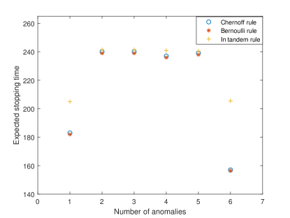
(a) Homogeneous case

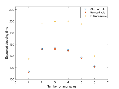
(b) Heterogeneous case

Figure 1: Expected value of the stopping time that corresponds to each of the three sampling rules versus the number of anomalous sources ($\alpha=\beta=10^{-3}$).

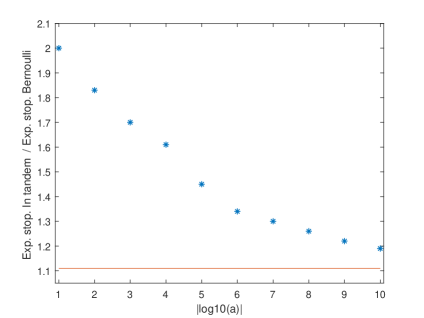
(a) $|A|=1$

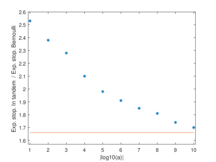
(b) $|A|=6$

Figure 2: In both graphs the $x$-axis represents $|\log_{10}(\alpha)|$ and the $y$-axis the ratio of the expected value of the stopping time implied by sampling in tandem over that implied by the asymptotically optimal Bernoulli rule in the homogeneous setup (70). The horizontal line refers to the value of (65).

In Figures 2 and 3 we plot the ratio of the expected value of the stopping time induced by sampling in tandem over that induced by the Bernoulli sampling rule against $|\log_{10}(\alpha)|$ as $\alpha$ ranges from $10^{-1}$ to $10^{-10}$. (We do not present the corresponding results for the Chernoff rule, as they are almost identical). Specifically, in Figure 2 we consider the homogeneous setup (70) when the number of anomalous sources is $1$ and $6$, whereas in Figure 3 we consider the heterogeneous setup (71) when the number of anomalous sources is $1,\,3,$ and 6. For each value of $\alpha$, the thresholds are selected according to (19) and each expectation is computed using $10^{4}$ simulation runs. The standard error for each estimated expectation is approximately $1$, whereas the standard error for each ratio is approximately $10^{-2}$ in the homogeneous setup and $3\cdot 10^{-2}$ in the heterogeneous setup. Moreover, in each case we plot the limiting value of this ratio, which is the limit defined in (62). In the homogeneous case this is given by (65) and is equal to

$$\begin{cases}10/\max\{10-1,\;5\}=10/9\approx 1.1&\;\text{when}\quad|A|=1,\\ 10/\max\{6,\;5\}=10/6\approx 1.6\;&\;\text{when}\quad|A|=6.\\ \end{cases}$$ (72)

In the heterogeneous case it is given by (66) and is equal to

$$\begin{cases}10/\max\{(1+0.25)\cdot 5-1,\;5\}=10/5.25\approx 1.9\;&\text{when}\quad|A|=1,\\ 10/\max\{(1+0.25)\cdot 5,\;5\}=10/6.25\approx 1.6\;&\text{when}\quad 1<|A|<6,\\ 10/\max\{(1-0.25)\cdot 5+0.25\cdot 6,\;5\}=10/5.25\approx 1.9\;&\text{when}\quad|A|=6.\end{cases}$$ (73)

From Figures 2 and 3 we can see that, in all cases, the efficiency loss due to sampling in tandem is (much) larger than the one suggested by the corresponding asymptotic relative efficiency when $\alpha$ is not (very) small.

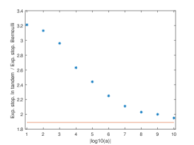
(a) $|A|=1$

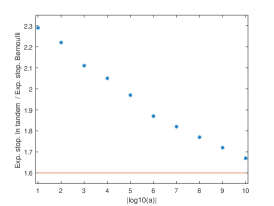
(b) $|A|=3$

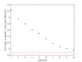
(c) $|A|=6$

Figure 3: In all graphs the $x$-axis represents $|\log_{10}(\alpha)|$ and the $y$-axis the ratio of the expected value of the stopping time implied by sampling in tandem over that implied by the asymptotically optimal Bernoulli rule in the heterogeneous setup (71). The horizontal line refers to the value of (66).

VIII Conclusions and extensions

In this paper we propose a novel formulation of the sequential anomaly detection problem with sampling constraints, in which arbitrary, user-specified bounds are assumed on the number of anomalous sources, the probabilities of at least one false alarm and at least one missed detection are controlled below distinct tolerance levels, and the number of sampled sources per time instance is not necessarily fixed. We obtain a general criterion for achieving the optimal expected time until stopping, to a first-order asymptotic approximation as the error probabilities go to 0, as long as the log-likelihood ratio statistic of each observation has a finite first moment. We show that asymptotic optimality is achieved, simultaneously under every possible subset of anomalous sources, for any version of the proposed problem, using the unmodified sampling rule in [20], to which we refer as Chernoff, but also using a novel sampling rule whose implementation requires minimal computations, to which we refer in this work as Bernoulli. Despite their very different computational requirements, these two rules are found in simulation studies to lead to essentially the same performance. On the other hand, it has been shown in simulation studies under various setups [12, 13, 16], that the Chernoff rule leads to significantly worse performance in practice compared to non-probabilistic sampling rules as the ones discussed in Subsection VI-C. The study of sampling rules of this nature in the general sequential anomaly detection framework we propose in this work is an interesting problem that we plan to consider in the future. Another interesting problem is that of establishing stronger than first-order asymptotic optimality, which has been solved in certain special cases of the sequential multi-hypothesis testing problem with controlled sensing [23, 24].

The results of this paper can be shown, using the techniques in [8], to remain valid for a variety of error metrics beyond the familywise error rates that we consider in this work, such as the false discovery rate and the false non-discovery rate. However, this is not the case for the generalized familywise error rates proposed in [31, 32], for which different policies and a different analysis is required. These error metrics have been considered in [4, 5, 7] in the case of full sampling, whereas certain results in the presence of sampling constraints have been presented in [33].

The results in this work can also be generalized in a natural way when the sampling cost varies per source, as in [15], or when the two hypotheses in each source are not completely specified, as it is done for example in [7] in the case of full sampling. Another potential generalization is the removal of the assumption that the acquired observations are conditionally independent of the past given the current sampling choice, as it is done in [27] in a general controlled sensing setup. Finally, another direction of interest is a setup where the focus is on the dependence structure of the sources rather than their marginal distributions, as for example in [34].

IX Acknowledgments

The authors would like to thank Prof. Venugopal Veeravalli for stimulating discussions.

Appendix A

In this Appendix we state and prove two auxiliary lemmas that are used in the proofs of various results of this paper. Specifically, we fix $A\in\mathcal{P}_{\ell,u}$, and for any $i\in[M]$, $n\in\mathbb{N}$ and any sampling rule $R$ we set

$$\begin{split}\widetilde{\Lambda}^{R}_{i}(n)&:=\widetilde{\Lambda}^{R}_{i}(n-1)+\Bigl{(}g_{i}(X_{i}(n))-\mathsf{E}_{A}[g_{i}(X_{i}(n))]\Bigr{)}\,R_{i}(n),\\ \widetilde{\Lambda}^{R}_{i}(0)&:=0,\end{split}$$ (74)

and comparing with (10) we observe that

$$\widetilde{\Lambda}^{R}_{i}(n) =\begin{cases}\Lambda^{R}_{i}(n)-I_{i}\,N^{R}_{i}(n),\quad i\in A\\ \Lambda^{R}_{i}(n)+J_{i}\,N^{R}_{i}(n),\quad i\notin A.\end{cases}$$ (75)

Lemma A.1

Let $R$ be an arbitrary sampling rule, $i\in A$, $j\notin A$, $\rho\in(0,1]$, and $\epsilon>0$. Then, the sequences

$$\mathsf{P}_{A}\left(\frac{1}{n}\Lambda^{R}_{i}(n)<\rho I_{i}-\epsilon,\;\pi_{i}^{R}(n)\geq\rho\right),$$

$$\mathsf{P}_{A}\left(\frac{1}{n}\Lambda^{R}_{j}(n)>-\rho J_{j}+\epsilon,\;\pi_{j}^{R}(n)\geq\rho\right),$$

$$\mathsf{P}_{A}\left(\frac{1}{n}\Lambda^{R}_{ij}(n)<\rho I_{i}-\epsilon,\;\pi^{R}_{i}(n)\geq\rho\right)$$

$$\mathsf{P}_{A}\left(\frac{1}{n}\Lambda^{R}_{ij}(n)<\rho J_{j}-\epsilon,\;\pi^{R}_{j}(n)\geq\rho\right)$$

are exponentially decaying.

Proof:

We prove the result for the third probability, as the proofs for the other ones are similar. To lighten the notation, we suppress the dependence on $R$ and we write $\widetilde{\Lambda}_{ij}(n),\widetilde{\Lambda}_{i}(n),\pi_{i}(n),\mathcal{F}_{n}$ instead of $\widetilde{\Lambda}^{R}_{ij}(n),\widetilde{\Lambda}^{R}_{i}(n),\pi_{i}^{R}(n),\mathcal{F}^{R}_{n}$. By (75), for every $n\in\mathbb{N}$ we have

$$\Lambda_{ij}(n) =\Lambda_{i}(n)-\Lambda_{j}(n)$$

$$=\widetilde{\Lambda}_{i}(n)-\widetilde{\Lambda}_{j}(n)+n(I_{i}\pi_{i}(n)+J_{j}\pi_{j}(n)),$$

which shows that if $\pi_{i}(n)\geq\rho$, then $\Lambda_{ij}(n)\geq\widetilde{\Lambda}_{i}(n)-\widetilde{\Lambda}_{j}(n)+n\rho I_{i}.$ Thus, for every $n\in\mathbb{N}$ we have

$$\mathsf{P}_{A}\left(\frac{1}{n}\Lambda_{ij}(n)<\rho I_{i}-\epsilon,\;\pi_{i}(n)\geq\rho\right)$$

$$\leq\mathsf{P}_{A}\left(\widetilde{\Lambda}_{i}(n)-\widetilde{\Lambda}_{j}(n)<-n\,\epsilon\right)$$

$$\leq\mathsf{P}_{A}\left(\widetilde{\Lambda}_{i}(n)<-n\,\epsilon/2\right)+\mathsf{P}_{A}\left(-\widetilde{\Lambda}_{j}(n)<-n\,\epsilon/2\right),$$

and it suffices to show that the two terms in the upper bound are exponentially decaying. We show this only for the first one, as the proof for the second is similar. For this, we fix $\delta\in(0,\epsilon/2)$ and we observe that, for any $t>0$ and $n\in\mathbb{N}$, by Markov’s inequality we have

$$\begin{split}&\mathsf{P}_{A}\left(\widetilde{\Lambda}_{i}(n)<-n\,\epsilon/2\right)\\ &\leq\exp\{-n\,t\,\epsilon/2\}\,\mathsf{E}_{A}\left[\exp\left\{-t\,\widetilde{\Lambda}_{i}(n)\right\}\right].\end{split}$$ (76)

By (74) and the law of iterated expectation it follows that the expectation in the upper bound can be written as follows:

$$\mathsf{E}_{A}\left[\exp\left\{-t\,\widetilde{\Lambda}_{i}(n-1)\right\}\cdot\mathsf{E}_{A}\left[\exp\left\{-t\,(g_{i}(X_{i}(n))-I_{i})\,R_{i}(n)\right\}\,|\,\mathcal{F}_{n-1}\right]\right].$$ (77)

Since $R(n)$ is an $\mathcal{F}_{n-1}$-measurable Bernoulli random variable and $X_{i}(n)$ is independent of $\mathcal{F}_{n-1}$ and has the same distribution as $X_{i}(1)$, we also have

$$\mathsf{E}_{A}\left[\exp\left\{-t\,(g_{i}(X_{i}(n))-I_{i})\,R_{i}(n)\right\}\,|\,\mathcal{F}_{n-1}\right]$$

$$=\mathsf{E}_{A}\left[\exp\left\{-t\,(g_{i}(X_{i}(1))-I_{i})\right\}\right]^{R_{i}(n)}$$

$$=\mathsf{E}_{A}\left[\exp\left\{t\,(-g_{i}(X_{i}(1))+I_{i}-\delta+\delta)\right\}\right]^{R_{i}(n)}$$

$$\leq\exp\left\{R_{i}(n)\,(\psi_{i}(t)+t\,\delta)\right\},$$

where $\psi_{i}$ is the cumulant generating function of $-g_{i}(X_{i}(1))+I_{i}-\delta$, i.e.,

$$\psi_{i}(t):=\log\mathsf{E}_{A}\left[\exp\left\{t(-g_{i}(X_{i}(1))+I_{i}-\delta)\right\}\right],\;t>0.$$

Since $\psi_{i}$ is convex on $(0,1)$, $\psi_{i}(1)=I_{i}-\delta<\infty$, and

$$\psi_{i}^{\prime}(0+)=\mathsf{E}_{A}[-g_{i}(X_{i}(1))+I_{i}-\delta]=-\delta<0,$$

there is an $s>0$ such that $\psi_{i}(s)<0$, and as a result

$$\exp\left\{R_{i}(n)\,(\psi_{i}(s)+s\,\delta)\right\} \leq\exp\left\{s\,\delta\right\}.$$

Therefore, setting $t=s$ in (76)-(77) we obtain

$$\mathsf{P}_{A}\left(\widetilde{\Lambda}_{i}(n)<-n\,\epsilon/2\right) \leq\exp\{-n\,(\epsilon/2)s+\delta s\}\;\mathsf{E}_{A}\left[\exp\left\{-s\,\widetilde{\Lambda}_{i}(n-1)\right\}\right].$$

Repeating the same argument $n-1$ times we conclude that there exists an $s>0$ such that

$$\mathsf{P}_{A}\left(\widetilde{\Lambda}_{i}(n)<-n\epsilon/2\right)\leq\exp\left\{-n(\epsilon/2-\delta)s\right\}.$$

Since $\delta\in(0,\epsilon/2)$, this completes the proof.
∎

Lemma A.2

Let $i\in A$, $j\notin A$, $\zeta>0$, $\rho_{i},\rho_{j}\in[0,1]$, and let $R$ be an arbitrary sampling rule.

• If $\rho_{i}>0$ and $\mathsf{P}_{A}(\pi_{i}^{R}(n)<\rho_{i})$ is summable, then so is

  $$\mathsf{P}_{A}\left(\frac{1}{n}\Lambda^{R}_{i}(n)<\rho_{i}I_{i}-\zeta\right).$$

• If $\rho_{j}>0$ and $\mathsf{P}_{A}(\pi_{j}^{R}(n)<\rho_{j})$ is summable, then so is

  $$\mathsf{P}_{A}\left(\frac{1}{n}\Lambda^{R}_{j}(n)>-\rho_{j}J_{j}+\zeta\right).$$

• If $\rho_{i}+\rho_{j}>0$ and both $\mathsf{P}_{A}(\pi_{j}^{R}(n)<\rho_{i})$ and $\mathsf{P}_{A}(\pi_{j}^{R}(n)<\rho_{j})$ are summable, then so is

  $$\mathsf{P}_{A}\left(\frac{1}{n}\Lambda^{R}_{ij}(n)<\rho_{i}I_{i}+\rho_{j}J_{j}-\zeta\right).$$

Proof:

For (i), by the law of total probability we have

$$\mathsf{P}_{A}\left(\frac{1}{n}\Lambda^{R}_{i}(n)<\rho_{i}I_{i}-\zeta\right)$$

$$\leq\mathsf{P}_{A}\left(\pi_{i}^{R}(n)<\rho_{i}\right)+\mathsf{P}_{A}\left(\frac{1}{n}\Lambda^{R}_{i}(n)<\rho_{i}I_{i}-\zeta,\,\pi^{R}_{i}(n)\geq\rho_{i}\right).$$

The first term in the upper bound is summable by assumption, whereas the second one is summable, as exponentially decaying, by Lemma A.1.

The proof of (ii) is similar and is omitted. Since (iii) follows directly by (i) and (ii) when $\rho_{i}$ and $\rho_{j}$ are both positive, it suffices to consider the case where only one them is positive. Without loss of generality, we assume that $\rho_{i}>0=\rho_{j}$. Then, by the law of total probability again we have

$$\mathsf{P}_{A}\left(\frac{1}{n}\Lambda^{R}_{ij}(n)<\rho_{i}I_{i}+\rho_{j}J_{j}-\zeta\right)$$

$$\leq\mathsf{P}_{A}\left(\pi_{i}^{R}(n)<\rho_{i}\right)+\mathsf{P}_{A}\left(\frac{1}{n}\Lambda^{R}_{ij}(n)<\rho_{i}I_{i}-\zeta,\,\pi^{R}_{i}(n)\geq\rho_{i}\right).$$

The first term in the upper bound is summable by assumption, whereas the second one is summable, as exponentially decaying, by Lemma A.1.
∎

Appendix B

In this Appendix we prove Theorems III.1 and IV.1, which provide sufficient conditions for the exponential consistency of a sampling rule. In order to lighten the notation, throughout this Appendix we suppress dependence on $R$ and we write $\pi_{i}(n)$, $\Lambda_{i}(n),\Lambda_{ij}(n),\Delta_{n}$, $c_{i}(A)$, $\sigma_{A}$ instead of $\pi_{i}^{R}(n)$, $\Lambda_{i}^{R}(n)$, $\Lambda_{ij}^{R}(n)$, $\Delta^{R}_{n}$, $c^{R}_{i}(A)$, $\sigma^{R}_{A}$.

Proof:

We prove the result first when $\ell=u$. By the definition of the decision rule in (13) it follows that when $\sigma_{A}>n$, there are $m\geq n$, $i\in A$, $j\notin A$ such that $\Lambda_{ij}(m)\leq 0$, and as a result by the union bound we have

$$\mathsf{P}_{A}(\sigma_{A}>n)\leq\sum\limits_{i\in A,\,j\notin A}\;\sum_{m=n}^{\infty}\mathsf{P}_{A}\left(\Lambda_{ij}(m)\leq 0\right).$$

Therefore, to show that $\mathsf{P}_{A}(\sigma_{A}>n)$ is exponentially decaying, it suffices to show that this is the case for $\mathsf{P}_{A}\left(\Lambda_{ij}(n)\leq 0\right)$ for every $i\in A$ and $j\notin A$. To show this, we fix such $i$ and $j$ and we note that, by assumption, either $\mathsf{P}_{A}(\pi_{i}(n)<\rho)$ or $\mathsf{P}_{A}(\pi_{j}(n)<\rho)$ is exponentially decaying for $\rho>0$ small enough. Without loss of generality, suppose that this is the case for the former. By an application of the law of total probability we then obtain

$$\mathsf{P}_{A}\left(\Lambda_{ij}(n)\leq 0\right) \leq\mathsf{P}_{A}(\Lambda_{ij}(n)\leq 0,\pi_{i}(n)\geq\rho)$$

$$+\mathsf{P}_{A}(\pi_{i}(n)<\rho).$$

As mentioned earlier, the second term in the upper bound is, by assumption, exponentially decaying for $\rho>0$ small enough. By Lemma A.1 it follows that this is also the case for the first one.

Suppose next that $\ell<|A|<u$. By the definition of the decision rule in (17) it follows that when $\sigma_{A}>n$, there is an $m\geq n$ such that either $\Lambda_{i}(m)<0$ for some $i\in A$, or $\Lambda_{j}(m)>0$ for some $j\notin A$. As a result, by the union bound we have

$$\mathsf{P}_{A}({\sigma}_{A}>n) \leq\sum\limits_{i\in A}\;\sum_{m=n}^{\infty}\mathsf{P}_{A}(\Lambda_{i}(m)<0)$$

$$+\sum\limits_{j\notin A}\;\sum_{m=n}^{\infty}\mathsf{P}_{A}(\Lambda_{j}(m)\geq 0).$$

Therefore, to prove that $\mathsf{P}_{A}(\sigma_{A}>n)$ is exponentially decaying, it suffices to show that this is true for $\mathsf{P}_{A}\left(\Lambda_{i}(n)<0\right)$ and $\mathsf{P}_{A}\left(\Lambda_{j}(n)\geq 0\right)$ for every $i\in A$ and $j\notin A$. This can be shown similarly to the case $\ell=u$, in view of the fact that the sequences $\mathsf{P}_{A}(\pi_{i}(n)<\rho)$ and $\mathsf{P}_{A}(\pi_{j}(n)<\rho)$ are, by assumption, both exponentially decaying for $\rho>0$ small enough and for every $i\in A$ and $j\notin A$.

The two remaining cases are $\ell<|A|=u$ and $\ell=|A|<u$. We consider only the former, as the proof for the latter is similar, and assume that $\ell<|A|=u$. By the definition of the decision rule in (13) it follows that when $\sigma_{A}>n$, there is an $m\geq n$ such that either $\Lambda_{ij}(m)\leq 0$ for some $i\in A$ and $j\notin A$, or $\Lambda_{i}(m)<0$ for some $i\in A$. As a result, by the union bound we have

$$\mathsf{P}_{A}(\sigma_{A}>\zeta n) \leq\sum\limits_{i\in A}\sum_{m=n}^{\infty}\mathsf{P}_{A}(\Lambda_{i}(m)<0)$$

$$+\sum\limits_{i\in A,j\notin A}\sum_{m=n}^{\infty}\mathsf{P}_{A}(\Lambda_{ij}(m)\leq 0).$$

Since $|A|>\ell$, the sequence $\mathsf{P}_{A}(\pi_{i}(n)<\rho)$ is, by assumption, exponentially decaying for every $i\in A$ and $\rho>0$ small enough. Therefore, similarly to the previous cases we can show that each term in the upper bound is exponentially decaying.
∎

In the remainder of this Appendix we prove Theorem IV.1, whose proof relies on two preliminary lemmas. To state those, for every $D\in\mathcal{P}_{\ell,u}$ and $n\in\mathbb{N}$ we denote by $\tau^{D}_{n}$ the first time instance $m$ at which $D$ has been estimated as the subset of anomalous sources for at least $2\,\zeta\,m$ times since $\lceil n/2\rceil$, i.e.

$$\tau^{D}_{n}:=\inf\left\{m\geq\lceil n/2\rceil:\sum_{u=\lceil n/2\rceil}^{m}\mathbf{1}\{\Delta_{u-1}=D\}\geq 2\zeta m\right\},$$ (78)

where $\zeta>0$ is an arbitrary constant, which in the proof of Theorem IV.1 will be selected to be small enough.

Lemma B.1

Let $D\in\mathcal{P}_{\ell,u}$ and $i\in[M]$. If $c_{i}(D)>0$, then $\mathsf{P}(\tau^{D}_{n}\leq n,\;\pi_{i}(\tau^{D}_{n})<\rho)$ and $\mathsf{P}(\tau^{D}_{n}\leq n,\;\pi_{i}(n)<\rho)$ are both exponentially decaying for all $\rho>0$ small enough.

Proof:

We prove the two claims together by showing that $\mathsf{P}(\tau^{D}_{n}\leq n,\;\pi_{i}(\sigma_{n})<\rho)$ is exponentially decaying for all $\rho>0$ small enough, where $\sigma_{n}$ stands for either $n$ or $\tau_{n}^{D}$. For any given $n\in\mathbb{N}$ we set

$$\widetilde{\pi}_{i}(n) :=\frac{1}{n}\sum_{m=1}^{n}(R_{i}(m)-c_{i}(\Delta_{m-1}))$$

$$=\pi_{i}(n)-\frac{1}{n}\sum_{m=1}^{n}c_{i}(\Delta_{m-1}),\quad n\in\mathbb{N}.$$

Then, on the event $\{\tau^{D}_{n}\leq n\}$ we have $n/2\leq\tau^{D}_{n}\leq\sigma_{n}\leq n$ and consequently

$$\pi_{i}(\sigma_{n})-\widetilde{\pi}_{i}(\sigma_{n}) =\frac{1}{\sigma_{n}}\sum_{m=1}^{\sigma_{n}}c_{i}(\Delta_{m-1})$$

$$\geq\frac{c_{i}(D)}{n}\sum_{m=\lceil n/2\rceil}^{\tau^{D}_{n}}\,\mathbf{1}\{\Delta_{m-1}=D\}$$

$$\geq\frac{c_{i}(D)}{n}\,2\,\zeta\,\tau_{n}^{D}\geq\;c_{i}(D)\,\zeta,$$

where in the last inequality we have used the definition of $\tau_{n}^{D}$. Consequently, for every $\rho>0$ and $n\in\mathbb{N}$ we obtain

$$\{\tau^{D}_{n}\leq n,\;\pi_{i}(\sigma_{n})\leq\rho\}\subseteq\{\tau^{D}_{n}\leq n,\,\widetilde{\pi}_{i}(\sigma_{n})\leq\rho-c_{i}(D)\,\zeta\}.$$

Since $c_{i}(D)>0$, there is an $\epsilon>0$ such that for all $\rho\in(0,c_{i}(D)\zeta-\epsilon)$ we have

$$\{\tau^{D}_{n}\leq n,\;\pi_{i}(\sigma_{n})\leq\rho\}\subseteq\left\{\max_{\lceil n/2\rceil\leq m\leq n}|\widetilde{\pi}_{i}(m)|\geq\epsilon\right\}.$$

Therefore, it suffices to show that, for all $\epsilon>0$, the sequence

$$\mathsf{P}\left(\max_{\lceil n/2\rceil\leq m\leq n}|\widetilde{\pi}_{i}(m)|\geq\epsilon\right)$$ (79)

is exponentially decaying. This follows by the fact that $(R_{i}(n)-c_{i}(\Delta_{n-1}))$ is a uniformly bounded martingale difference, in view of (22), and an application of the maximal Azuma-Hoeffding submartingale inequality [35, Remark 2.3].
∎

Lemma B.2

Let $A,D\in\mathcal{P}_{\ell,u}$ be such that $|D|\in\{l,u\}$ and $D\neq A$. If $R$ is a sampling rule that satisfies the conditions of Theorem IV.1, then the sequence $\mathsf{P}_{A}(\tau^{D}_{n}\leq n)$ is exponentially decaying.

Proof:

We consider first the case that $\ell<u$, where we only prove the result when $|D|=u$, as the proof when $|D|=\ell$ is similar. Since $A\in\mathcal{P}_{\ell,u}$, $|D|=u$ and $D\neq A$, there exists a $j\in D\setminus A$. Since also $|D|>\ell$, the assumptions of Theorem IV.1 imply that $c_{j}(D)>0$. Thus, by Lemma B.1 it follows that

$$\mathsf{P}_{A}\left(\tau^{D}_{n}\leq n,\;\pi_{j}(\tau^{D}_{n})<\rho\right)$$ (80)

is an exponentially decaying sequence for $\rho>0$ small enough, and it suffices to show that this is also the case for

$$\mathsf{P}_{A}\left(\tau^{D}_{n}\leq n,\;\;\pi_{j}(\tau^{D}_{n})\geq\rho\right).$$ (81)

Indeed, by the definition of $\tau^{D}_{n}$ in (78) it follows that on the event $\{\tau^{D}_{n}<\infty\}$ we have $\Delta(\tau_{n}^{D}-1)=D$. Since $|D|=u$ and $j\in D$, by the definition of the decision rule in (17) it follows that $\Lambda_{j}(\tau^{D}_{n}-1)>0$. Therefore,

$$\begin{split}&\mathsf{P}_{A}\left(\tau^{D}_{n}\leq n,\;\;\pi_{j}(\tau^{D}_{n})\geq\rho\right)\\ &=\mathsf{P}_{A}(\tau^{D}_{n}\leq n,\,\Lambda_{j}(\tau_{n}^{D}-1)>0,\,\pi_{j}(\tau_{n}^{D})\geq\rho)\\ &\leq\sum_{m=\lceil n/2\rceil}^{n}\mathsf{P}_{A}\left(\Lambda_{j}(m-1)>0,\,\pi_{j}(m)\geq\rho\right),\end{split}$$

where the inequality holds because $\tau_{n}^{D}$ takes values in $[n/2,n]$ on the event $\{\tau_{n}^{D}\leq n\}$. Therefore, it remains to show that the sequence

$$\mathsf{P}_{A}\left(\Lambda_{j}(n-1)>0,\,\pi_{j}(n)\geq\rho\right)$$ (82)

is exponentially decaying for $\rho>0$ small enough. Indeed, for large enough $n$, $\pi_{j}(n)\geq\rho$ implies that

$$\pi_{j}(n-1)\geq\frac{n\pi_{j}(n)-1}{n-1}\geq\frac{\rho n-1}{n-1}\geq\rho-\frac{1}{n-1}.$$

For any given $\rho>0$, there exists a $\rho^{\prime}>0$ so that for all $n$ large enough we have

$$\rho-\frac{1}{n-1}>\rho^{\prime},$$ (83)

and so that the probability in (82) is bounded by

$$\mathsf{P}_{A}\left(\Lambda_{j}(n-1)>0,\,\pi_{j}(n-1)\geq\rho^{\prime}\right).$$

For $\rho>0$ small enough, $\rho^{\prime}>0$ is small enough, and by Lemma A.1 it follows that the latter probability, and consequently (82), is exponentially decaying in $n$.

It remains to prove the lemma when $\ell=u$ and $A\neq D$. In this case there are $i\in A\setminus D$ and $j\in D\setminus A$, and by the assumptions of Theorem IV.1 it follows that either $c_{i}(D)>0$ or $c_{j}(D)>0$. Without loss of generality, we assume that the latter holds. Then, by Lemma B.1 it follows that (80) is exponentially decaying for all $\rho>0$ small enough, and it suffices to show that this is also the case for (81). Indeed, by the definition of $\tau^{D}_{n}$ in (78) it follows that on the event $\{\tau^{D}_{n}<\infty\}$ we have $\Delta(\tau_{n}^{D}-1)=D$. Consequently, by the definition of the decision rule in (13) it follows that there is an $i\in A\setminus D$ such that $\Lambda_{ij}(\tau^{D}_{n}-1)<0$. Therefore, by the union bound we have

$$\mathsf{P}_{A}\left(\tau^{D}_{n}\leq n,\;\;\pi_{j}(\tau^{D}_{n})\geq\rho\right)$$

$$=\sum_{i\in A\setminus D}\mathsf{P}_{A}\left(\tau^{D}_{n}\leq n,\,\Lambda_{ij}(\tau^{D}_{n}-1)<0,\,\pi_{j}(\tau_{n}^{D})\geq\rho\right)$$

$$\leq\sum_{i\in A\setminus D}\sum_{m=\lceil n/2\rceil}^{n}\mathsf{P}_{A}\left(\Lambda_{ij}(m-1)<0,\,\pi_{j}(m)\geq\rho\right),$$

where as before the inequality holds because $\tau_{n}^{D}$ takes values in $[n/2,n]$ on the event $\{\tau_{n}^{D}\leq n\}$. Therefore, it remains to show that the sequence

$$\mathsf{P}_{A}\left(\Lambda_{ij}(n-1)<0,\,\pi_{j}(n)\geq\rho\right)$$

is exponentially decaying for $\rho>0$ small enough. As before, this follows by an application of Lemma A.1. ∎

Proof:

Fix $A\in\mathcal{P}_{\ell,u}$. By Theorem III.1 it suffices to show that, for all $\rho>0$ small enough, $\mathsf{P}_{A}(\pi_{i}(n)<\rho)$ is an exponentially decaying sequence

• for every $i\in A$, if $|A|>\ell$, and for every $i\notin A$, if $|A|<u$, when $\ell<u$,

• either for every $i\in A$ or for every $i\notin A$, when $\ell=u$.

In order to do so, we select the positive constant $\zeta$ in (78) to be smaller than $1/|\mathcal{P}_{\ell,u}|$. Then, for every $n\in\mathbb{N}$ there is at least one $D\in\mathcal{P}_{\ell,u}$ for which $\{\tau^{D}_{n}\leq n\}\neq\emptyset$. As a result, for every $i\in[M]$ and $\rho>0$, by the union bound we have

$$\mathsf{P}_{A}(\pi_{i}(n)<\rho)\leq\sum_{D\in\mathcal{P}_{\ell,u}}\mathsf{P}_{A}\left(\pi_{i}(n)<\rho,\;\tau_{n}^{D}\leq n\right).$$

Suppose first that $\ell<u$. Then, it suffices to show that, for every $D\in\mathcal{P}_{\ell,u}$ and all $\rho>0$ small enough,

$$\mathsf{P}_{A}\left(\pi_{i}(n)<\rho,\tau_{n}^{D}\leq n\right)$$ (84)

is exponentially decaying for every $i\in A$ when $|A|>\ell$ and for every $i\notin A$ when $|A|<u$. We only consider the former case, as the proof for the latter is similar. Thus, suppose that $|A|>\ell$ and let $i\in A$.

• If $c_{i}(D)>0$, by Lemma B.1 it follows that (84) is an exponentially decaying sequence.

• If $c_{i}(D)=0$, the assumption of the theorem implies that either $|D|=u$ and $i\notin D$, or $|D|=\ell$ and $i\in D$. In either case, $A\neq D$ and by Lemma B.2 it follows that $\mathsf{P}_{A}(\tau_{n}^{D}\leq n)$, and consequently (84), is an exponentially decaying sequence.

Suppose now that $\ell=u$. Then, it suffices to show that (84) is exponentially decaying for every $D\in\mathcal{P}_{\ell,u}$ and all $\rho>0$ small enough, either for every $i\in A$ or for every $i\notin A$.

• When $D\neq A$, by Lemma B.2 it follows that $\mathsf{P}_{A}(\tau_{n}^{D}\leq n)$, and consequently (84), is exponentially decaying.

• When $D=A$, then by assumption $c_{i}(A)>0$ holds either for every $i\in A$ or for every $i\notin A$. By Lemma B.1 it then follows that (84) is exponentially decaying either for every $i\in A$ or for every $i\notin A$, and this completes the proof.

∎

Appendix C

In this Appendix we fix $A\in\mathcal{P}_{\ell,u}$ and prove the universal asymptotic lower bound of Theorem V.2. The proof relies on two lemmas, for the statement of which we need to introduce the following function:

$$\phi(\alpha,\beta):=\alpha\log\left(\frac{\alpha}{1-\beta}\right)+(1-\alpha)\log\left(\frac{1-\alpha}{\beta}\right),$$

where $\alpha,\beta\in(0,1)$, i.e., the Kullback-Leibler divergence between a Bernoulli distribution with parameter $\alpha$ and one with parameter $1-\beta$. Moreover, we set $\phi(\alpha)\equiv\phi(\alpha,\alpha)$.

The first lemma states a non-asymptotic, information-theoretic inequality that generalizes the one used in Wald’s universal lower bound in the problem of testing two simple hypotheses [36, p. 156].

Lemma C.1

Let $\alpha+\beta<1$ and let $(R,T,\Delta)$ be a policy that satisfies the error constraint (3) and $\mathsf{P}_{A}(T<\infty)=1$. Then, for any $C\in\mathcal{P}_{\ell,u}$ such that $C\neq A$ we have

$$\mathsf{E}_{A}\left[\Lambda^{R}_{A,{C}}(T)\right]\geq\begin{cases}\phi(\alpha,\beta)\;&\text{if }\;{C}{\setminus}A\neq\emptyset,\mbox{ }A{\setminus}{C}=\emptyset,\\ \phi(\beta,\alpha)\;&\text{if }\;{C}{\setminus}A=\emptyset,\mbox{ }A{\setminus}{C}\neq\emptyset,\\ \phi(\alpha\wedge\beta)\quad&\text{if }\;{C}{\setminus}A\neq\emptyset,\mbox{ }A{\setminus}{C}\neq\emptyset.\end{cases}$$ (85)

Proof:

The proof is identical to that in the full sampling case in [6, Theorem 5.1], and can be obtained by an application of the data processing inequality for Kullback-Leibler divergences (see, e.g., [37, Lemma 3.2.1]). Indeed, the left-hand side is the Kullback-Leibler divergence between $\mathsf{P}_{A}$ and $\mathsf{P}_{C}$ given the available information up to time $T$, when the sampling rule $R$ is utilized, whereas the right hand side is obtained by considering the Kullback-Leibler divergence between $\mathsf{P}_{A}$ and $\mathsf{P}_{C}$ based on a single event of $\mathcal{F}^{R}_{T}$. ∎

We next make use of the previous inequality to establish lower bounds on the expected number of samples taken from each source until stopping.

Lemma C.2

Let $\alpha+\beta<1$ and let $(R,T,\Delta)$ be a policy that satisfies the error constraint (3) and $\mathsf{E}_{A}[T]<\infty$.

1. If $|A|<u$, then

   $$\min_{j\notin A}\left(J_{j}\,\mathsf{E}_{A}\left[N_{j}^{R}(T)\right]\right)\geq\phi(\alpha,\beta).$$ (86)

2. If $|A|>\ell$, then

   $$\min_{i\in A}\left(I_{i}\,\mathsf{E}_{A}\left[N_{i}^{R}(T)\right]\right)\geq\phi(\beta,\alpha).$$ (87)

3. If either $|A|=\ell>0$ or $|A|=u<M$, then

   $$\min_{i\in A}\left(I_{i}\,\mathsf{E}_{A}\left[N_{i}^{R}(T)\right]\right)+\min_{j\notin A}\left(J_{j}\,\mathsf{E}_{A}\left[N_{j}^{R}(T)\right]\right)\geq\phi(\alpha\wedge\beta).$$ (88)

Proof:

We recall the sequence $\widetilde{\Lambda}^{R}_{i},$ defined in (74), and note that it is a zero-mean, $\{\mathcal{F}^{R}_{n}\}$-martingale under $\mathsf{P}_{A}$. Moreover, by the finiteness of the Kullback-Leibler divergences in (1) we have:

$$\sup_{n\in\mathbb{N}}\mathsf{E}_{A}\left[|\widetilde{\Lambda}^{R}_{i}(n)-\widetilde{\Lambda}^{R}_{i}(n-1)|\;|\;\mathcal{F}^{R}_{n-1}\right]<\infty.$$

Since also $T$ is an $\{\mathcal{F}^{R}_{n}\}$-stopping time such that $\mathsf{E}_{A}[T]<\infty$, by the Optional Sampling Theorem [38, pg. 251] we obtain:

$$\mathsf{E}_{A}\left[\widetilde{\Lambda}^{R}_{i}(T)\right]=0\quad\text{for every}\quad i\in[M].$$ (89)

(i) If $|A|<u$, there is a $j\notin A$ such that $C=A\cup\{j\}\in\mathcal{P}_{\ell,u}$. By representation (11) and decomposition (75) it follows that the log-likelihood ratio process in (9) takes the form

$$\Lambda_{A,C}^{R}(T)=-\Lambda_{j}^{R}(T)=-\widetilde{\Lambda}_{j}^{R}(T)+J_{j}\,N_{j}^{R}(T).$$

By (85) and (89) we then obtain

$$J_{j}\,\mathsf{E}_{A}\left[N_{j}^{R}(T)\right]\geq\phi(\alpha,\beta).$$

Since this inequality holds for every $j\notin A$, this completes the proof.

(ii) The proof is similar to (i) and is omitted.

(iii) If $|A|=\ell>0$ or $|A|=u<M$, then there are $i\in A$ and $j\notin A$ such that $C=A\cup\{j\}\setminus\{i\}\in\mathcal{P}_{\ell,u}$. By representation (11) and decomposition (75) we have

$$\Lambda^{R}_{A,C}(T) =\Lambda_{i}^{R}(T)-\Lambda_{j}^{R}(T)$$

$$=\widetilde{\Lambda}_{i}^{R}(T)-\widetilde{\Lambda}^{R}_{j}(T)+J_{j}\,N_{j}^{R}(T)+I_{i}\,N_{i}^{R}(T).$$

By (85) and (89) we then obtain

$$I_{i}\,\mathsf{E}_{A}\left[N_{i}^{R}(T)\right]+J_{j}\,\mathsf{E}_{A}\left[N_{j}^{R}(T)\right]\geq\phi(\alpha\wedge\beta).$$

Since this inequality holds for every $i\in A$ and $j\notin A$, this proves (88).
∎

For the proof of Theorem V.1 we introduce the following notation:

$$\begin{split}\mathcal{D}_{K}&:=\left\{(c_{1},\ldots,c_{M})\in[0,1]^{M}:\sum_{i=1}^{M}c_{i}\leq K\right\}\\ \mathcal{D}^{\prime}_{K}&:=\{(p,q)\in[0,1]^{2}:\;p\hat{K}_{A}+q\check{K}_{A}\leq K\}.\end{split}$$ (90)

Moreover, we observe that as $\alpha,\beta\to 0$ we have

$$\phi(\alpha,\beta) \sim|\log\beta|,$$ (91)

$$r(\alpha,\beta)\equiv\frac{\phi(\beta,\alpha)}{\phi(\alpha,\beta)} \sim\frac{|\log\alpha|}{|\log\beta|}.$$ (92)

Proof:

(i) Let $\alpha,\beta\in(0,1)$ such that $\alpha+\beta<1$ and $(R,T,\Delta)\in\mathcal{C}(\alpha,\beta,\ell,u,K)$ such that $\mathsf{E}_{A}[T]<\infty$. By Lemma C.2(iii) it then follows that

$$\mathsf{E}_{A}[T]\;W_{A}(T)\geq\phi(\alpha\wedge\beta),\quad\text{where}$$

$$W_{A}(T) :=\min_{i\in A}\left\{I_{i}\,\frac{\mathsf{E}_{A}[N^{R}_{i}[T]}{\mathsf{E}_{A}[T]}\right\}+\min_{j\notin A}\left\{J_{j}\,\frac{\mathsf{E}_{A}[N^{R}_{j}[T]}{\mathsf{E}_{A}[T]}\right\},$$

and by constraint (4) we conclude that

$$\mathsf{E}_{A}[T]\;V_{A} \geq\phi(\alpha\wedge\beta),$$

$$\text{where}\qquad V_{A} :=\max_{(c_{1},\ldots,c_{M})\in\mathcal{D}_{K}}\left\{\min\limits_{i\in A}(c_{i}I_{i})+\min\limits_{j{\notin}A}(c_{j}J_{j})\right\}.$$

Since the lower bound is independent of the policy $(R,T,D)$, we have

$$\mathcal{J}_{A}(\alpha,\beta,\ell,u,K)\;V_{A} \geq\phi(\alpha\wedge\beta).$$

Comparing with (30) and recalling (91), we can see that it suffices to show that $V_{A}=x_{A}I_{A}^{*}+y_{A}J_{A}^{*}$ with $x_{A}$ and $y_{A}$ as in (31)-(32). Indeed, the maximum in $V_{A}$ is achieved by $c_{i}$’s of the form

$$\begin{split}c_{i}I_{i}&=pI_{A}^{*},\quad i\in A,\\ c_{j}J_{j}&=qJ_{A}^{*},\quad j\notin A,\end{split}$$ (93)

for $p,q\in[0,1]$ such that the constraint in $\mathcal{D}_{K}$ is satisfied, i.e.,

$$K\geq\sum_{i=1}^{M}c_{i}=p\sum_{i\in A}\frac{I^{*}_{A}}{I_{i}}+q\sum_{j\notin A}\frac{J^{*}_{A}}{J_{j}}=p\,\hat{K}_{A}+q\,\check{K}_{A},$$ (94)

and as a result,

$$V_{A}=\max_{(p,q)\in\mathcal{D}^{\prime}_{K}}\{pI_{A}^{*}+qJ_{A}^{*}\}.$$

This maximum is achieved by $p,q\in[0,1]$ such that $p\hat{K}_{A}+q\check{K}_{A}=K\wedge(\hat{K}_{A}+\check{K}_{A})$, in particular by $p$ and $q$ equal to $x_{A}$ and $y_{A}$ as in (31)-(32), which completes the proof.

(ii) Suppose first that $\ell<|A|<u$. As before, let $\alpha,\beta\in(0,1)$ such that $\alpha+\beta<1$ and $(R,T,\Delta)\in\mathcal{C}(\alpha,\beta,\ell,u,K)$ such that $\mathsf{E}_{A}[T]<\infty$. Then, by Lemma C.2(i) and Lemma C.2(ii) we obtain:

$$\mathsf{E}_{A}[T]\;W_{A}(T)\geq\phi(\beta,\alpha),\;\text{where}$$

$$W_{A}(T) :=\min\left\{\min_{i\in A}\left\{I_{i}\,\frac{\mathsf{E}_{A}[N^{R}_{i}[T]}{\mathsf{E}_{A}[T]}\right\},\;r(\alpha,\beta)\;\min_{j\notin A}\left\{J_{j}\,\frac{\mathsf{E}_{A}[N^{R}_{j}[T]}{\mathsf{E}_{A}[T]}\right\}\right\},$$

and by constraint (4) we conclude that

$$\begin{split}&\mathsf{E}_{A}[T]\;V_{A}(\alpha,\beta)\geq\phi(\beta,\alpha)\\ \text{where}\qquad V_{A}(\alpha,\beta)&:=\max_{(c_{1},\ldots,c_{M})\in\mathcal{D}_{K}}\min\left\{\min_{i\in A}\left(c_{i}I_{i}\right),\,r(\alpha,\beta)\;\min_{j\notin A}\left(c_{j}J_{j}\right)\right\}.\end{split}$$ (95)

Since the lower bound does not depend on the policy $(R,T,\Delta)$ we have

$$\mathcal{J}_{A}(\alpha,\beta,\ell,u,K)\;V_{A}(\alpha,\beta) \geq\phi(\beta,\alpha).$$

Comparing with (33) and recalling (91) we can see that it suffices to show that

$$V_{A}(\alpha,\beta)\rightarrow x_{A}\,I_{A}^{*}=r\,y_{A}\,J_{A}^{*}$$

as $\alpha,\beta\to 0$ according to (7), with $x_{A}$ and $y_{A}$ as in (33). The equality follows directly from the values of $x_{A}$ and $y_{A}$ in (35). Moreover, the maximum in $V_{A}(\alpha,\beta)$ is achieved by $c_{1},\ldots,c_{M}$ of the form (93) that satisfy (94). Therefore:

$$V_{A}(\alpha,\beta)=\max_{(p,q)\in\mathcal{D}^{\prime}_{K}}\min\left\{pI_{A}^{*},\,r(\alpha,\beta)\,qJ_{A}^{*}\right\},$$

and this maximum is achieved for $p$ and $q$ such that the two terms in the minimum are equal. As a result, we obtain

$$V_{A}(\alpha,\beta)=pI_{A}^{*}=r(\alpha,\beta)\,qJ_{A}^{*},$$

where $p$ and $q$ are equal to $x_{A}$ and $y_{A}$ in (33), with $r$ replaced by $r(\alpha,\beta)$. As $\alpha$ and $\beta$ go to $0$ according to (7), we have $r(\alpha,\beta)\to r$ (recall (92)), and consequently $V_{A}(\alpha,\beta)\rightarrow x_{A}\,I_{A}^{*}$ with $x_{A}$ as in (35).

Finally, we consider the case $|A|=\ell$ and omit the proof when $|A|=u$, as it is similar. When either $\ell=0$ or $r\leq 1$, we have to show (34). Indeed, working as before, using Lemma C.2(i), we obtain

$$\mathcal{J}_{A}(\alpha,\beta,\ell,u,K)\;V_{A} \geq\phi(\alpha,\beta),$$

$$\text{where}\quad V_{A} :=\max_{(c_{1},\ldots,c_{M})\in\mathcal{D}_{K}}\;\min_{j\notin A}\;\left\{c_{j}J_{j}\right\}.$$

Comparing with (34), and recalling (91), we can see that it suffices to show that $V_{A}=J_{A}^{*}\;y_{A},$ with $y_{A}$ as in (34). Indeed, the maximum in $V_{A}$ is achieved by $c_{1},\ldots,c_{M}$ of the form (93) with $p=0$ and $q\in[0,1]$ such that (94) is satisfied, i.e.,

$$V_{A}=J_{A}^{*}\;\max_{q\in[0,1]:\;q\check{K}_{A}\leq K}q,$$

which shows that $V_{A}=J_{A}^{*}\;y_{A},$ with $y_{A}$ as in (34) and completes the proof in this case.

It remains to establish the asymptotic lower bound when $\ell>0$ and $r>1$, in which case we have to show (35)-(36). The asymptotic equivalence in (35) can be shown by direct evaluation, therefore it suffices to show only the asymptotic lower bound in this case.

Working as before, using Lemma C.2(i) and Lemma C.2(iii), for any $\alpha,\beta\in(0,1)$ such that $\alpha+\beta<1$ we obtain

$$\begin{split}&\mathcal{J}_{A}(\alpha,\beta,\ell,u,K)\;\;V_{A}(\alpha,\beta)\geq\phi(\beta,\alpha),\quad\text{where}\\ V_{A}(\alpha,\beta)&:=\max_{(c_{1},\ldots,c_{M})\in\mathcal{D}_{K}}\min\left\{r(\alpha,\beta)\;\min_{j\notin A}\left(c_{j}J_{j}\right),\,\min_{i{\in}A}\left(c_{i}I_{i}\right)+\min_{j\notin A}\left(c_{j}J_{j}\right)\right\}.\end{split}$$ (96)

The latter maximum is achieved by $c_{1},\ldots,c_{M}$ of the form (93) that satisfy (94), thus,

$$V_{A}(\alpha,\beta) =\max_{(p,q)\in\mathcal{D}^{\prime}_{K}}\;\min\left\{r(\alpha,\beta)\;qJ_{A}^{*},\;pI_{A}^{*}+qJ_{A}^{*}\right\}.$$

• If $\theta_{A}\geq r(\alpha,\beta)-1$ or $K\leq\hat{K}_{A}+(\theta_{A}/(r(\alpha,\beta)-1))\check{K}_{A}$, the maximum in $V_{A}(\alpha,\beta)$ is achieved when the two terms in the minimum are equal. As a result, we have

  $$V_{A}(\alpha,\beta)=p\,I_{A}^{*}+q\,J_{A}^{*}=r(\alpha,\beta)\;qJ_{A}^{*}$$ (97)

  with $p$ and $q$ equal to $x_{A}$ and $y_{A}$ as in (35), but with $r$ replaced by $r(\alpha,\beta)$.

• Otherwise, the second term in the minimum is smaller and the first equality in (97) holds with $p$ and $q$ equal to $x_{A}$ and $y_{A}$ as in (36), but with $r$ replaced by $r(\alpha,\beta)$.

Therefore, letting $\alpha$ and $\beta$ go to 0 in (96) according to (7), and recalling (91)-(92), proves the asymptotic lower bounds in both (35) and (36).

∎

Appendix D

In this Appendix we prove Theorems V.2 and V.3, which provide sufficient conditions for asymptotic optimality. In both proofs we recall that: $c_{i}^{*}(A)>0$ for every $i$ in $A$ (resp. $A^{c}$) when $x_{A}>0$ (resp. $y_{A}>0$), $x_{A}\vee y_{A}>0$, $x_{A}>0$ when $|A|>\ell$, and $y_{A}>0$ when $|A|<u$.

Proof:

We prove the theorem first when $\ell=u$, where $\alpha$ and $\beta$ go to 0 at arbitrary rates. By the asymptotic lower bound (30) in Theorem V.1 it follows that in this case it suffices to show

$$\mathsf{E}_{A}[T^{R}]\lesssim\frac{|\log(\alpha\wedge\beta)|}{x_{A}\,I_{A}^{*}+y_{A}\,J_{A}^{*}}.$$ (98)

Then, for any $\epsilon>0$ small enough and $c>0$ we set

$$L_{\epsilon}(c):=\max_{i\in A,j\notin A}\frac{c}{(c_{i}^{*}(A)-\epsilon)I_{i}+(c_{j}^{*}(A)-\epsilon)J_{j}-\epsilon},$$ (99)

and observe that

$$\mathsf{E}_{A}[T^{R}]\leq L_{\epsilon}(c)+\sum_{n>L_{\epsilon}(c)}\mathsf{P}_{A}(T^{R}>n).$$ (100)

For any $n\in\mathbb{N}$, by the definition of $T^{R}$ in (12) it follows that on the event $\{T^{R}>n\}$ there are $i\in A$ and $j\notin A$ such that $\Lambda^{R}_{ij}(n)<c$, and as a result

$$\mathsf{P}_{A}(T^{R}>n) \leq\sum_{i\in A,j\notin A}\mathsf{P}_{A}(\Lambda^{R}_{ij}(n)<c).$$

Moreover, for any $n>L_{\epsilon}(c)$ and $i\in A,j\notin A$ we have

$$c<n\left((c_{i}^{*}(A)-\epsilon)I_{i}+(c_{j}^{*}(A)-\epsilon)J_{j}-\epsilon\right),$$ (101)

and consequently for every $c>0$ the series in (100) is bounded by

$$\sum_{i\in A,j\notin A}\sum_{n=1}^{\infty}\mathsf{P}_{A}\left(\frac{\Lambda^{R}_{ij}(n)}{n}<(c_{i}^{*}(A)-\epsilon)I_{i}+(c_{j}^{*}(A)-\epsilon)J_{j}-\epsilon\right).$$ (102)

By the assumption of the theorem and an application of Lemma A.2(iii) with $\rho_{i}$ equal to $c_{i}^{*}(A)-\epsilon$ (resp. $0$) when $x_{A}>0$ (resp. $x_{A}=0$) and $\rho_{j}$ equal to $c_{j}^{*}(A)-\epsilon$ (resp. $0$) when $y_{A}>0$ (resp. $y_{A}=0$), it follows that the series in (102) converges. Thus, letting first $c\to\infty$ and then $\epsilon\to 0$ in (100) proves that as $c\to\infty$ we have

$$\mathsf{E}_{A}[T^{R}]\lesssim\max_{i\in A,j\notin A}\frac{c}{c_{i}^{*}(A)I_{i}+c_{j}^{*}(A)\,J_{j}}.$$ (103)

In view of (40) and the selection of threshold $c$ according to (18), this proves (98).

We next consider the case $\ell<u$, where we let $\alpha,\beta\to 0$ so that (7) holds for some $r\in(0,\infty)$. We prove the result when $\ell\leq|A|<u$, as the proof when $\ell<|A|\leq u$ is similar. Thus, in what follows, $\ell\leq|A|<u$, and as a result $y_{A}>0$ and $c_{j}^{*}(A)>0$ for every $j\notin A$. By the universal asymptotic lower bounds (33) and (34) it follows that when either $|A|>\ell$ or $|A|=\ell=0$, it suffices to show that

$$\mathsf{E}_{A}[T^{R}]\lesssim\frac{|\log\beta|}{y_{A}\,J^{*}_{A}}.$$ (104)

On the other hand, by the universal asymptotic lower bounds (35) and (36) it follows that when $|A|=\ell>0$, it suffices to show that

$$\mathsf{E}_{A}[T^{R}]\lesssim\frac{|\log\beta|}{y_{A}J_{A}^{*}}\bigvee\frac{|\log\alpha|}{x_{A}I_{A}^{*}+y_{A}J_{A}^{*}}.$$ (105)

When in particular $r\leq 1$, the maximum is attained strictly by the first term, when $r>1$, $z_{A}<1$ and $K>\hat{K}_{A}+z_{A}\check{K}_{A}$, the maximum is attained strictly by the second term, whereas in all other cases the two terms are equal to a first-order asymptotic approximation.

We start by proving (104) when $\ell<|A|<u$. In this case we also have $x_{A}>0$, and consequently $c_{i}^{*}(A)>0$ for every $i\in A$. Then, for $\epsilon>0$ small enough and $a,\,b>0$ we set

$$N_{\epsilon}(a,b):=\max_{j\notin A,\,i\in A}\left\{\frac{a}{(c_{j}^{*}(A)-\epsilon)J_{j}-\epsilon},\,\frac{b}{(c_{i}^{*}(A)-\epsilon)I_{i}-\epsilon}\right\},$$ (106)

and observe that

$$\mathsf{E}_{A}[T^{R}]\leq N_{\epsilon}(a,b)+\sum_{n>N_{\epsilon}(a,b)}\mathsf{P}_{A}(T^{R}>n).$$ (107)

By the definition of $T^{R}$ in (16) it follows that, for any $n\in\mathbb{N}$, on the event $\{T^{R}>n\}$ there is either a $j\notin A$ such that $\Lambda^{R}_{j}(n)>-a$, or an $i\in A$ such that $\Lambda^{R}_{i}(n)<b$. As a result, by the union bound we obtain

$$\mathsf{P}_{A}(T^{R}>n) \leq\sum_{j\notin A}\mathsf{P}_{A}(-\Lambda^{R}_{j}(n)<a)+\sum_{i\in A}\mathsf{P}_{A}(\Lambda^{R}_{i}(n)<b).$$

Moreover, for any $n>N_{\epsilon}(a,b)$ and any $i\in A$, $j\notin A$ we have $a<n((c_{j}^{*}(A)-\epsilon)J_{j}-\epsilon)$ and $b<n((c_{i}^{*}(A)-\epsilon)I_{i}-\epsilon)$, which implies that the series in (107) is bounded by

$$\begin{split}&\sum_{j\notin A}\sum_{n=1}^{\infty}\mathsf{P}_{A}\left(-\frac{1}{n}\Lambda^{R}_{j}(n)<(c_{j}^{*}(A)-\epsilon)J_{j}-\epsilon\right)\\ &+\sum_{i\in A}\sum_{n=1}^{\infty}\mathsf{P}_{A}\left(\frac{1}{n}\Lambda^{R}_{i}(n)<(c_{i}^{*}(A)-\epsilon)I_{i}-\epsilon\right).\end{split}$$ (108)

By the assumption of the theorem and an application of Lemma A.2(i) with $\rho_{i}=c_{i}^{*}(A)-\epsilon$ and of Lemma A.2(ii) with $\rho_{j}=c_{j}^{*}(A)-\epsilon$ it follows that (108) converges. Thus, letting first $a,\,b\to\infty$ and then $\epsilon\to 0$ in (107) proves that as $a,\,b\to\infty$

$$\mathsf{E}_{A}[T^{R}]\lesssim\max_{j\notin A,\,i\in A}\left\{\frac{a}{c_{j}^{*}(A)J_{j}},\,\frac{b}{c_{i}^{*}(A)I_{i}}\right\}.$$

In view of (40) and the selection of thresholds $a,b$ according to (19), this implies that

$$\mathsf{E}_{A}[T^{R}]\lesssim\frac{|\log\beta|}{y_{A}\,J^{*}_{A}}\sim\frac{|\log\alpha|}{x_{A}\,I^{*}_{A}},$$ (109)

and proves (104).

The proof when $|A|=\ell=0$, in which case $x_{A}=0$, is similar, with the difference that we use

$$N_{\epsilon}(a):=\max_{j\notin A}\left\{\frac{a}{(c_{j}^{*}(A)-\epsilon)J_{j}-\epsilon}\right\}$$ (110)

in the place of $N_{\epsilon}(a,c)$, and apply only Lemma A.2(i).

It remains to show that (105) holds when $|A|=\ell>0$, in which case $x_{A}$ is not always positive. We recall the definitions of $L_{\epsilon}(c)$ and $N_{\epsilon}(a)$ in (99) and (110) and observe that for any $\epsilon>0$ small enough and $a,c>0$ we have

$$\mathsf{E}_{A}[T^{R}]\leq L_{\epsilon}(c)\vee N_{\epsilon}(a)+\sum_{n>L_{\epsilon}(c)\vee N_{\epsilon}(a)}\mathsf{P}_{A}(T^{R}>n).$$ (111)

By the definition of $T^{R}$ in (16) it follows that, for any $n\in\mathbb{N}$, on the event $\{T^{R}>n\}$ there are either $i\in A$ and $j\notin A$ such that $\Lambda^{R}_{ij}(n)<c$ or $j\notin A$ such that $\Lambda^{R}_{j}(n)>-a$, and as a result

$$\mathsf{P}_{A}(T^{R}>n) \leq\sum_{i\in A,j\notin A}\mathsf{P}_{A}(\Lambda^{R}_{ij}(n)<c)+\sum_{j\notin A}\mathsf{P}_{A}(\Lambda^{R}_{j}(n)>-a).$$

Following similar steps as in the previous cases, applying in particular Lemma A.2(ii) with $\rho_{j}=c_{j}^{*}(A)-\epsilon$ and Lemma A.2(iii) with $\rho_{j}=c_{j}^{*}(A)-\epsilon$ and $\rho_{i}$ equal to $c_{i}^{*}(A)-\epsilon$ (resp. $0$) when $x_{A}>0$ (resp. $x_{A}=0$), we conclude that as $a,c\to\infty$

$$\mathsf{E}_{A}[T^{R}]\lesssim\max_{i\in A,j\notin A}\left\{\frac{a}{c_{j}^{*}(A)J_{j}}\bigvee\frac{c}{c_{i}^{*}(A)I_{i}+c_{j}^{*}(A)J_{j}}\right\}.$$

In view of (40) and the selection of thresholds $a,c$ according to (19), this proves (105).
∎

Proof:

Fix $A\in\mathcal{P}_{\ell,u}$ and a probabilistic sampling rule $R$ that satisfies (45). Since $c_{i}^{*}(A)>0$ for every $i$ in $A$ (resp. $A^{c}$) when $x_{A}>0$ (resp. $y_{A}>0$), $x_{A}\vee y_{A}>0$, $x_{A}>0$ when $|A|>\ell$, and $y_{A}>0$ when $|A|<u$, the exponentially consistency of $R$ under $\mathsf{P}_{A}$ follows by an application of Theorem IV.1. To establish its asymptotic optimality, by Theorem V.2 it follows that it suffices to show that $\mathsf{P}_{A}(\pi_{i}^{R}(n)<\rho)$ is an exponentially decaying sequence for every $\rho\in(0,c_{i}^{*}(A))$ and $i\in[M]$ such that $c_{i}^{*}(A)>0$. Fix such $i$ and $\rho$. Then, there is an $\epsilon>0$ such that

$$\rho+\epsilon<c_{i}^{*}(A).$$ (112)

By the definition of a probabilistic rule (recall (21)), $R(n+1)$ is conditionally independent of $\mathcal{F}_{n}^{R}$ given $\Delta_{n}^{R}$ and its conditional distribution, $q^{R}$, does not depend on $n$. Thus, by [39, Prop. 6.13] there is a measurable function $h:\mathcal{P}_{\ell,u}\times[0,1]\to 2^{[M]}$, which does not depend on $n$, such that

$$R(n+1)=h\left(\Delta_{n}^{R},Z_{0}(n)\right),\quad n\in\mathbb{N},$$

where $\{Z_{0}(n),n\in\mathbb{N}\}$ is a sequence of iid random variables, uniformly distributed in $(0,1)$. Consequently, there is a measurable function $h_{i}:\mathcal{P}_{\ell,u}\times[0,1]\to\{0,1\}$ such that

$$R_{i}(n+1)=h_{i}\left(\Delta_{n}^{R},Z_{0}(n)\right),\quad n\in\mathbb{N}.$$ (113)

Then, for every $n\in\mathbb{N}$ we have

$$\{\pi_{i}^{R}(n)<\rho\} =\left\{\sum_{m=1}^{n}h_{i}\left(A,Z_{0}(m-1)\right)+\sum_{m=1}^{n}(R_{i}(m)-h_{i}(A,Z_{0}(m-1))<n(\rho+\epsilon)-n\epsilon\right\},$$

and as a result

$$\begin{split}\mathsf{P}_{A}(\pi_{i}^{R}(n)<\rho)&\leq\mathsf{P}_{A}\left(\sum_{m=1}^{n}h_{i}(A,Z_{0}(m-1))<n(\rho+\epsilon)\right)\\ &+\mathsf{P}_{A}\left(\sum_{m=1}^{n}(R_{i}(m)-h_{i}(A,Z_{0}(m-1)))<-n\epsilon\right).\end{split}$$ (114)

From (22) and (113) it follows that $\{h_{i}(A,Z_{0}(n-1)),n\in\mathbb{N}\}$ is a sequence of iid Bernoulli random variables with parameter $c^{R}_{i}(A)$, whereas by (45) and (112) it follows that $\rho+\epsilon<c^{R}_{i}(A)$. Therefore, by the Chernoff bound we conclude that the first term in the upper bound in (114) is exponentially decaying. The second term is bounded as follows

$$\mathsf{P}_{A}\left(\sum_{m=1}^{n}(R_{i}(m)-h_{i}(A,Z_{0}(m-1)))<-n\epsilon\right)$$

$$\leq\mathsf{P}_{A}\left(\sum_{m=1}^{n}|R_{i}(m)-h_{i}(A,Z_{0}(m-1))|>n\epsilon\right)$$

$$\leq\mathsf{P}_{A}\left(\sigma^{R}_{A}>n\right)+\mathsf{P}_{A}\left(\sigma^{R}_{A}>n\epsilon\right),$$ (115)

where the first inequality follows from the triangle inequality and the second by an application of the total probability rule on the event $\{\sigma^{R}_{A}\leq n\}$, in view of the fact that

$$\sigma^{R}_{A}\leq n\quad\Rightarrow\quad\sum_{m=1}^{n}|R_{i}(m)-h_{i}(A,Z_{0}(m-1))|\leq\sigma^{R}_{A}.$$

By the exponentially consistency of $R$, the upper bound in (D) is exponentially decaying, which means that the second term in the upper bound in (114) is also exponentially decaying, and this completes the proof. ∎

References

• [1] J. Stiles and T. Jernigan, “The basics of brain development,” Neuropsychology review, vol. 20, pp. 327–48, 11 2010.
• [2] R. J. Bolton and D. J. Hand, “Statistical Fraud Detection: A Review,” Statistical Science, vol. 17, no. 3, pp. 235 – 255, 2002. [Online]. Available: https://doi.org/10.1214/ss/1042727940
• [3] S. K. De and M. Baron, “Sequential bonferroni methods for multiple hypothesis testing with strong control of family-wise error rates i and ii,” Sequential Analysis, vol. 31, no. 2, pp. 238–262, 2012.
• [4] ——, “Step-up and step-down methods for testing multiple hypotheses in sequential experiments,” Journal of Statistical Planning and Inference, vol. 142, no. 7, pp. 2059–2070, 2012.
• [5] J. Bartroff and J. Song, “Sequential tests of multiple hypotheses controlling type i and ii familywise error rates,” Journal of statistical planning and inference, vol. 153, pp. 100–114, 2014.
• [6] Y. Song and G. Fellouris, “Asymptotically optimal, sequential, multiple testing procedures with prior information on the number of signals,” Electronic Journal of Statistics, vol. 11, 03 2016.
• [7] ——, “Sequential multiple testing with generalized error control: An asymptotic optimality theory,” The Annals of Statistics, vol. 47, no. 3, pp. 1776 – 1803, 2019. [Online]. Available: https://doi.org/10.1214/18-AOS1737
• [8] J. Bartroff and J. Song, “Sequential tests of multiple hypotheses controlling false discovery and nondiscovery rates,” Sequential Analysis, vol. 39, no. 1, pp. 65–91, 2020. [Online]. Available: https://doi.org/10.1080/07474946.2020.1726686
• [9] K. S. Zigangirov, “On a problem in optimal scanning,” Theory of Probability & Its Applications, vol. 11, no. 2, pp. 294–298, 1966. [Online]. Available: https://doi.org/10.1137/1111025
• [10] E. M. Klimko and J. Yackel, “Optimal search strategies for wienér processes,” Stochastic Processes and their Applications, vol. 3, pp. 19–33, 1975.
• [11] V. Dragalin, “A simple and effective scanning rule for a multi-channel system,” Metrika, vol. 43, pp. 165–182, 02 1996.
• [12] K. Cohen and Q. Zhao, “Asymptotically optimal anomaly detection via sequential testing,” IEEE Transactions on Signal Processing, vol. 63, no. 11, pp. 2929–2941, 2015.
• [13] B. Huang, K. Cohen, and Q. Zhao, “Active anomaly detection in heterogeneous processes,” IEEE Transactions on Information Theory, vol. 65, no. 4, pp. 2284–2301, 2019.
• [14] N. K. Vaidhiyan and R. Sundaresan, “Learning to detect an oddball target,” IEEE Transactions on Information Theory, vol. 64, no. 2, pp. 831–852, 2018.
• [15] A. Gurevich, K. Cohen, and Q. Zhao, “Sequential anomaly detection under a nonlinear system cost,” IEEE Transactions on Signal Processing, vol. 67, no. 14, pp. 3689–3703, 2019.
• [16] A. Tsopelakos, G. Fellouris, and V. V. Veeravalli, “Sequential anomaly detection with observation control,” in 2019 IEEE International Symposium on Information Theory (ISIT), 2019, pp. 2389–2393.
• [17] B. Hemo, T. Gafni, K. Cohen, and Q. Zhao, “Searching for anomalies over composite hypotheses,” IEEE Transactions on Signal Processing, vol. 68, pp. 1181–1196, 2020.
• [18] H. Chernoff, “Sequential design of experiments,” Ann. Math. Statist., vol. 30, no. 3, pp. 755–770, 09 1959. [Online]. Available: http://dx.doi.org/10.1214/aoms/1177706205
• [19] A. E. Albert, “The Sequential Design of Experiments for Infinitely Many States of Nature,” The Annals of Mathematical Statistics, vol. 32, no. 3, pp. 774 – 799, 1961. [Online]. Available: https://doi.org/10.1214/aoms/1177704973
• [20] S. A. Bessler, “Theory and applications of the sequential design of experiments, k-actions and infinitely many experiments, part i theory.” Department of Statistics, Stanford University, Technical Report 55, 1960.
• [21] ——, “Theory and applications of the sequential design of experiments, k-actions and infinitely many experiments, part ii applications.” Department of Statistics, Stanford University, Technical Report 56, 1960.
• [22] J. Kiefer and J. Sacks, “Asymptotically Optimum Sequential Inference and Design,” The Annals of Mathematical Statistics, vol. 34, no. 3, pp. 705 – 750, 1963. [Online]. Available: https://doi.org/10.1214/aoms/1177704000
• [23] R. Keener, “Second Order Efficiency in the Sequential Design of Experiments,” The Annals of Statistics, vol. 12, no. 2, pp. 510 – 532, 1984. [Online]. Available: https://doi.org/10.1214/aos/1176346503
• [24] S. P. Lalley and G. Lorden, “A Control Problem Arising in the Sequential Design of Experiments,” The Annals of Probability, vol. 14, no. 1, pp. 136 – 172, 1986. [Online]. Available: https://doi.org/10.1214/aop/1176992620
• [25] S. Nitinawarat, G. K. Atia, and V. V. Veeravalli, “Controlled sensing for multihypothesis testing,” IEEE Transactions on Automatic Control, vol. 58, no. 10, pp. 2451–2464, 2013.
• [26] M. Naghshvar and T. Javidi, “Active sequential hypothesis testing,” The Annals of Statistics, vol. 41, no. 6, pp. 2703–2738, 2013.
• [27] S. Nitinawarat and V. V. Veeravalli, “Controlled sensing for sequential multihypothesis testing with controlled markovian observations and non-uniform control cost,” Sequential Analysis, vol. 34, no. 1, pp. 1–24, 2015. [Online]. Available: https://doi.org/10.1080/07474946.2014.961864
• [28] A. Deshmukh, V. V. Veeravalli, and S. Bhashyam, “Sequential controlled sensing for composite multihypothesis testing,” Sequential Analysis, vol. 40, no. 2, pp. 259–289, 2021. [Online]. Available: https://doi.org/10.1080/07474946.2021.1912525
• [29] A. Garivier and E. Kaufmann, “Optimal best arm identification with fixed confidence,” in Conference on Learning Theory.   PMLR, 2016, pp. 998–1027.
• [30] S. I. Resnick, Adventures in stochastic processes.   Springer Science & Business Media, 1992.
• [31] G. Hommel and T. Hoffmann, “Controlled uncertainty,” in Multiple Hypothesenprüfung/Multiple Hypotheses Testing.   Springer, 1988, pp. 154–161.
• [32] E. L. Lehmann and J. P. Romano, “Generalizations of the familywise error rate,” Ann. Statist., vol. 33, no. 3, pp. 1138–1154, 06 2005. [Online]. Available: http://dx.doi.org/10.1214/009053605000000084
• [33] A. Tsopelakos and G. Fellouris, “Sequential anomaly detection with observation control under a generalized error metric,” in 2020 IEEE International Symposium on Information Theory (ISIT), 2020, pp. 1165–1170.
• [34] J. Heydari, A. Tajer, and H. V. Poor, “Quickest linear search over correlated sequences,” IEEE Transactions on Information Theory, vol. 62, no. 10, pp. 5786–5808, 2016.
• [35] M. Raginsky and I. Sason, “Concentration of measure inequalities in information theory, communications, and coding,” Foundations and Trends® in Communications and Information Theory, vol. 10, no. 1-2, pp. 1–246, 2013. [Online]. Available: http://dx.doi.org/10.1561/0100000064
• [36] A. Wald, “Sequential tests of statistical hypotheses,” The Annals of Mathematical Statistics, vol. 16, no. 2, pp. 117–186, 1945.
• [37] A. Tartakovsky, I. Nikiforov, and M. Basseville, Sequential analysis: Hypothesis testing and changepoint detection.   CRC press, 2015.
• [38] Y. Chow and H. Teicher, Probability Theory: Independence, Interchangeability, Martingales, ser. Springer Texts in Statistics.   Springer New York, 2012. [Online]. Available: https://books.google.com/books?id=213dBwAAQBAJ
• [39] O. Kallenberg, Foundations of Modern Probability, ser. Probability and Its Applications.   Springer New York, 2002. [Online]. Available: https://books.google.com/books?id=TBgFslMy8V4C