Learning Robust Output Control Barrier Functions from Safe Expert Demonstrations

Abstract

This paper addresses learning safe output feedback control laws from partial observations of expert demonstrations. We assume that a model of the system dynamics and a state estimator are available along with corresponding error bounds, e.g., estimated from data in practice. We first propose robust output control barrier functions (ROCBFs) as a means to guarantee safety, as defined through controlled forward invariance of a safe set. We then formulate an optimization problem to learn ROCBFs from expert demonstrations that exhibit safe system behavior, e.g., data collected from a human operator or an expert controller. When the parametrization of the ROCBF is linear, then we show that, under mild assumptions, the optimization problem is convex. Along with the optimization problem, we provide verifiable conditions in terms of the density of the data, smoothness of the system model and state estimator, and the size of the error bounds that guarantee validity of the obtained ROCBF. Towards obtaining a practical control algorithm, we propose an algorithmic implementation of our theoretical framework that accounts for assumptions made in our framework in practice. We empirically validate our algorithm in the autonomous driving simulator CARLA and demonstrate how to learn safe control laws from RGB camera images.

1 Introduction

Safety-critical systems rely on robust control laws that can account for uncertainties in system dynamics and state estimation. For example, consider an autonomous car equipped with noisy sensors that navigates through urban traffic [1]. The state of the car is not exactly known and estimated from output measurements, e.g., from a dashboard camera, while the dynamics of the car are not perfectly known either, e.g., due to unknown friction coefficients. A model of the system dynamics and a state estimator can usually be obtained, e.g., from first principles or estimated from data, along with uncertainty sets describing error bounds. Such error bounds are standard in robust control theory [2], but designing robust control laws in this setting is challenging. In this paper, we address this problem by using the increasing availability of safe expert demonstrations, e.g., car manufacturers recording safe driving behavior of expert drivers. We propose a data-driven approach to learning safe and robust control laws where safety is defined as the ability of a system to stay within a set of states that are labeled safe, e.g., states that satisfy a minimum safety distance.

1.1 Related Work

Control barrier functions (CBFs) were introduced in [3, 4] to render a safe set controlled forward invariant. A CBF defines a set of safe control inputs that can be used to find a minimally invasive safety-preserving correction to a nominal control law by solving a convex quadratic program. Many variations and extensions of CBFs appeared in the literature, e.g., composition of CBFs [5], CBFs for multi-robot systems [6], CBFs encoding temporal logic constraints [7], and CBFs for systems with higher relative degree [8].

CBFs that account for uncertainties in the system dynamics have been considered in two ways. The authors in [9] and [10] consider input-to-state safety to quantify possible safety violation. Conversely, the work in [11] proposes robust CBFs to guarantee robust safety by accounting for all permissible errors within an uncertainty set. CBFs that account for state estimation uncertainties were proposed in [12] and [13]. Relying on the same notion of measurement robust CBFs as in [12], the authors in [14] present empirical evaluations on a segway. While the notion of ROCBFs that we present in this paper is inspired by measurement-robust CBFs as presented in [12], we also consider uncertainties in the system dynamics and focus on learning valid CBFs from expert demonstrations. Similar to the notion of ROCBF, the authors in [15] consider additive disturbances in the system dynamics and state-estimation errors jointly. We, however, consider more general forms of uncertainties.

Learning with CBFs: Approaches that use CBFs during learning typically assume that a valid CBF is already given, while we focus on constructing CBFs so that our approach can be viewed as complementary. In [16], it is shown how safe and optimal reward functions can be obtained, and how these are related to CBFs. The authors in [17] use CBFs to learn a provably correct neural network safety guard for kinematic bicycle models. The authors in [18] consider that uncertainty enters the system dynamics linearly and propose to use robust adaptive CBFs, as originally presented in [19], in conjunction with online set membership identification methods. In [20], it is shown how additive and multiplicative noise can be estimated online using Gaussian process regression for safe CBFs. The authors in [21] collect data to episodically update the system model and the CBF controller. A similar idea is followed in [22] where instead a projection with respect to the CBF condition is episodically learned. Imitation learning under safety constraints imposed by a Lyapunov function was proposed in [23]. Further work in this direction can be found in [24, 25, 26].

Learning CBFs: An open problem is how valid CBFs can be constructed. Indeed, the lack of systematic methods to constructs valid CBFs is a main bottleneck. For certain types of mechanical systems under input constraints, analytic CBFs can be constructed [27]. The construction of polynomial barrier functions towards certifying safety for polynomial systems by using sum-of-squares (SOS) programming was proposed in [28]. Finding CBFs poses additional challenges in terms of the control input resulting in bilinear SOS programming as presented in [29, 30] and summarized in [31]. The work in [32] considers the construction of higher order CBFs and their composition by, similarly to [29, 30], alternating-descent heuristics to solve the arising bilinear SOS program. Such SOS-based approaches, however, are known to be limited in scalability and do not use potentially available expert demonstrations.

A promising research direction is to learn CBFs from data. The authors in [33] construct CBFs from safe and unsafe data using support vector machines, while authors in [34] learn as set of linear CBFs for clustered datasets. The authors in [35] proposed learning limited duration CBFs and the work in [36] learns signed distance fields that define a CBF. In [37], a neural network controller is trained episodically to imitate an already given CBF. The authors in [38] learn parameters associated with the constraints of a CBF to improve feasibility. These works present empirical validations, but no formal correctness guarantees are provided. The authors in [39, 40, 41, 42] propose counter-example guided approaches to learn Lyapunov and barrier functions for known closed-loop systems, while Lyapunov functions for unknown systems are learned in [43]. In [44] and [45] control barrier functions are learned and post-hoc verified using Lipschitz arguments and satisfiability modulo theory. As opposed to these works, we make use of safe expert demonstrations. Expert trajectories are utilized in [46] to learn a contraction metric along with a tracking controller, while motion primitives are learned from expert demonstrations in [47]. In our previous work [48], we proposed to learn CBFs for known nonlinear systems from expert demonstrations. We provided the first conditions that ensure correctness of the learned CBF using Lipschitz continuity and covering number arguments. In [49] and [50], we extended this framework to partially unknown hybrid systems. In this paper, we focus on state estimation and provide sophisticated simulations of our method in CARLA.

1.2 Contributions

In this paper, we learn safe output feedback control laws for unknown systems. We first present robust output control barrier functions (ROCBFs) to establish safety under system dynamics and state estimation uncertainties. We then formulate a constrained optimization problem for constructing ROCBFs from safe expert demonstrations, and we present verifiable conditions that guarantee the validity of the ROCBF. While the optimization problem is in general nonconvex, we identify conditions under which the problem is convex. For the general case, we propose an approximate unconstrained optimization problem that we can solve efficiently. Finally, we propose an algorithmic implementation of our theoretical framework to learn ROCBFs in practice, and we present an empirical validation in CARLA [51].

In contrast to our previous works [48, 50, 49], in which we assume perfect state knowledge, we focus on dealing with state estimation errors. Our paper additionally differs from [48, 50, 49] in its practical focus. We discuss the algorithmic implementation of our framework to account for assumptions of our work in practice. For instance, our framework crucially relies on obtaining “unsafe” data which is hard to obtain in practice, and we propose a new algorithm to obtain unsafe datapoints as boundary points from the set of safe expert demonstrations based on reverse $k$-nearest neighbors.

2 Background and Problem Formulation

At time $t\in\mathbb{R}_{\geq 0}$, let $x(t)\in\mathbb{R}^{n}$ be the state of the dynamical control system described by the set of equations

$$\dot{x}(t) =f(t)+g(t)u(t),$$ (1a)

$$x(0) :=x_{0}\,\;\;\;\;\;\;\;\;\;\;\;\;\;\;\;\;\;\,\text{(initial condition),}$$ (1b)

$$f(t) :=F(x(t),t)\,\;\;\;\;\;\;\,\text{(internal dynamics),}$$ (1c)

$$g(t) :=G(x(t),t)\,\;\;\;\;\;\;\,\text{(input dynamics),}$$ (1d)

$$y(t) :=Y(x(t))\;\;\;\;\;\;\;\;\;\;\text{(output measurements),}$$ (1e)

$$u(t) :=U(y(t),t)\;\;\;\;\;\;\,\,\text{(output feedback control law),}$$ (1f)

where $x_{0}\in\mathbb{R}^{n}$ is the initial condition. The functions $F:\mathbb{R}^{n}\times\mathbb{R}_{\geq 0}\to\mathbb{R}^{n}$ and $G:\mathbb{R}^{n}\times\mathbb{R}_{\geq 0}\to\mathbb{R}^{n\times m}$ are only partially known, e.g., due to unmodeled dynamics or noise, and locally Lipschitz continuous in the first and piecewise continuous and bounded in the second argument.

Assumption 1.

We assume known nominal models $\hat{F}:\mathbb{R}^{n}\times\mathbb{R}_{\geq 0}\to\mathbb{R}^{n}$ and $\hat{G}:\mathbb{R}^{n}\times\mathbb{R}_{\geq 0}\to\mathbb{R}^{n\times m}$ together with functions $\Delta_{F}:\mathbb{R}^{n}\times\mathbb{R}_{\geq 0}\to\mathbb{R}_{\geq 0}$ and $\Delta_{G}:\mathbb{R}^{n}\times\mathbb{R}_{\geq 0}\to\mathbb{R}_{\geq 0}$ that bound their respective errors as

$$\|\hat{F}(x,t)-F(x,t)\| \leq\Delta_{F}(x,t)\text{ for all }(x,t)\in\mathbb{R}^{n}\times\mathbb{R}_{\geq 0},$$

$${|\kern-1.07639pt|\kern-1.07639pt|\hat{G}(x,t)-G(x,t)|\kern-1.07639pt|\kern-1.07639pt|} \leq\Delta_{G}(x,t)\text{ for all }(x,t)\in\mathbb{R}^{n}\times\mathbb{R}_{\geq 0}.$$

The functions $\hat{F}(x,t)$, $\hat{G}(x,t)$, $\Delta_{F}(x,t)$ and $\Delta_{G}(x,t)$ are assumed to be locally Lipschitz continuous in the first and piecewise continuous and bounded in the second argument.

The models $\hat{F}(x,t)$ and $\hat{G}(x,t)$ may be obtained by identifying model parameters or by system identification [52], while the assumption of error bounds $\Delta_{F}(x,t)$ and $\Delta_{G}(x,t)$ is standard in robust control [2]. We now define the set of admissible system dynamics as

$$\mathcal{F}(x,t) :=\{f\in\mathbb{R}^{n}|\|\hat{F}(x,t)-f\|\leq\Delta_{F}(x,t)\},$$

$$\mathcal{G}(x,t) :=\{g\in\mathbb{R}^{n\times m}|{|\kern-1.07639pt|\kern-1.07639pt|\hat{G}(x,t)-g|\kern-1.07639pt|\kern-1.07639pt|}\leq\Delta_{G}(x,t)\}.$$

The output measurement map $Y:\mathbb{R}^{n}\to\mathbb{R}^{p}$ is only partially known and locally Lipschitz continuous. For instance, $Y$ can describe a dashboard camera that is hard to model. We assume that there exists an inverse yet unknown map $X:\mathbb{R}^{p}\to\mathbb{R}^{n}$ that recovers the state $x$ as $X(Y(x))=x$. This means that a measurement $y$ uniquely defines a corresponding state $x$ and implies that $p\geq n$. This way, we implicitly assume high-dimensional measurements $y$ such as a dashboard camera where the inverse map $X$ recovers the position of the system, or even its velocity when a sequence of camera images is available. Since $Y$ and $X$ are unknown, one can, however, not recover the state $x$ from $y$. We present an example in the simulation study and refer to related literature using similar assumptions, such as [12, 53].

Assumption 2.

We assume to have a known model $\hat{X}:\mathbb{R}^{p}\to\mathbb{R}^{n}$ together with a function $\Delta_{X}:\mathbb{R}^{p}\to\mathbb{R}_{\geq 0}$ that bounds the error

$$\|\hat{X}(y)-X(y)\| \leq\Delta_{X}(y)\text{ for all }y\in Y(\mathbb{R}^{n}).$$

The functions $\hat{X}(y)$ and $\Delta_{X}(y)$ are assumed to be locally Lipschitz continuous.

The state estimator $\hat{X}(y)$ and the error bound $\Delta_{X}(y)$ may be obtained using machine learning methods, see e.g., [12, 53], or $\hat{X}(y)$ can encode the extended Kalman filter together with $\Delta_{X}(y)$, see e.g., [54, 55]. We now define the set of admissible inverse output measurement maps as

$$\mathcal{X}(y) :=\{x\in\mathbb{R}^{n}|\|\hat{X}(y)-x\|\leq\Delta_{X}(y)\}.$$

Finally, the function $U:\mathbb{R}^{p}\times\mathbb{R}_{\geq 0}\to\mathcal{U}$ is the output feedback control law where $\mathcal{U}\subseteq\mathbb{R}^{m}$ encodes input constraints. System (1) is illustrated in Fig. 1. Let a solution to (1) under an output feedback control law $U(y,t)$ be $x:\mathcal{I}\to\mathbb{R}^{n}$ where $\mathcal{I}\subseteq\mathbb{R}_{\geq 0}$ is the maximum definition interval of $x$.

Figure 1: Uncertain system under consideration.

The goal in this paper is to learn an output feedback control law $U(y,t)$ such that prescribed safety properties with respect to a geometric safe set $\mathcal{S}\subseteq\mathbb{R}^{n}$ are met by the system in (1). By geometric safe set, we mean that $\mathcal{S}$ describes the set of safe states as naturally specified on a subset of the state space (e.g., to avoid collision, vehicles must maintain a minimum separating distance).

Definition 1.

A set $\mathcal{C}\subseteq\mathbb{R}^{n}$ is said to be robustly output controlled forward invariant with respect to the system in (1) if there exist an output feedback control law $U(y,t)$ such that, for all initial conditions $x(0)\in\mathcal{C}$, for all admissible system dynamics $F(x,t)\in\mathcal{F}(x,t)$ and $G(x,t)\in\mathcal{G}(x,t)$, and for all admissible inverse output measurement maps $X(y)\in\mathcal{X}(y)$, every solution $x(t)$ to (1) under $U(y,t)$ is such that: 1) $x(t)\in\mathcal{C}$ for all $(t)\in\mathcal{I}$, and 2) the interval $\mathcal{I}$ is unbounded, i.e., $\mathcal{I}=[0,\infty)$. If the set $\mathcal{C}$ is additionally contained within the geometric safe set $\mathcal{S}$, i.e., $\mathcal{C}\subseteq\mathcal{S}$, the system in (1) is said to be safe under the safe control law $U(y,t)$.

Towards this goal, we assume a data set of expert demonstrations consisting of $N_{1}$ input-output data pairs $(y_{i},u_{i})\in\mathbb{R}^{p}\times\mathbb{R}^{m}$ along with a time stamp $t_{i}\in\mathbb{R}_{\geq 0}$ as

$$Z_{\mathrm{dyn}}:=\{(y_{i},t_{i},u_{i})\}_{i=1}^{N_{1}}$$

that were recorded when the system was in a safe state $X(y_{i})\in\text{int}(\mathcal{S})$ where $\text{int}(\cdot)$ denotes the interior of a set. We have expert control inputs $u_{i}$ available for each $y_{i}$ so that these can later be used for learning a safe control law.

Problem 1.

Let the system in (1) and the set of safe expert demonstrations $Z_{\mathrm{dyn}}$ be given. Under Assumptions 1 and 2, learn a function $h:\mathbb{R}^{n}\to\mathbb{R}$ from $Z_{\mathrm{dyn}}$ so that the set

$$\mathcal{C}:=\{x\in\mathbb{R}^{n}\,\big{|}\,h(x)\geq 0\}$$ (2)

is robustly output controlled forward invariant with respect to (1) and such that $\mathcal{C}\subseteq\mathcal{S}$, i.e., so that (1) is safe.

An overview of our proposed solution is shown in Fig. 2. We formulate a constrained optimization problem to learn a function $h(x)$ so that the learned safe set $\mathcal{C}$ is robustly output controlled forward invariant and contained within the geometric safe set $\mathcal{S}$, i.e., $\mathcal{C}\subseteq\mathcal{S}$. The optimization problem takes the system model $\mathcal{M}:=(\hat{F},\hat{G},\hat{X},\Delta_{F},\Delta_{G},\Delta_{X})$ and the expert demonstrations $\{(y_{i},u_{i},t_{i})\}$ as inputs and imposes constraints on $h(x)$ that will be derived in the sequel. We remark that the proofs of technical lemmas, propositions, and theorems can be found in the appendices.

Figure 2: Proposed framework to learn safe control laws.

3 Robust Output Control Barrier Functions

Let $h:\mathbb{R}^{n}\to\mathbb{R}$ be a twice continuously differentiable function, and assume that $h$ is such that the set $\mathcal{C}$ in (2) has non-empty interior. Let $\mathcal{Y}\subseteq\mathbb{R}^{p}$ be a sufficiently large open set such that $\mathcal{Y}\supseteq Y(\mathcal{C})$ where $Y(\mathcal{C})$ denotes the image of $\mathcal{\mathcal{C}}$ under $Y$. This assumption is equivalent to $X(\mathcal{Y})\supseteq C$. The set $X(\mathcal{Y})$ is typically the domain of interest in existing state-based CBF frameworks, see e.g., [4].

We recall that a function $\alpha:\mathbb{R}\to\mathbb{R}$ is an extended class $\mathcal{K}$ function if it is a strictly increasing function with $\alpha(0)=0$. We can guarantee that $\mathcal{C}$ is robustly output controlled forward invariant if there exists a locally Lipschitz continuous extended class $\mathcal{K}$ function $\alpha:\mathbb{R}\to\mathbb{R}$ such that

$$\begin{split}\sup_{u\in\mathcal{U}}\inf_{x\in\mathcal{X}(y)}\inf_{\begin{subarray}{c}f\in\mathcal{F}(x,t)\\ g\in\mathcal{G}(x,t)\end{subarray}}&\underbrace{\langle\nabla h(x),f+gu\rangle}_{\begin{subarray}{c}\text{Change in }h\text{ along}\\ \text{true dynamics}\end{subarray}}+\alpha(h(x))\geq 0\end{split}$$ (3)

for all $(y,t)\in\mathcal{Y}\times\mathbb{R}_{\geq 0}$ where $\langle\cdot,\cdot\rangle$ denotes the inner-product between two vectors. Unfortunately, the condition (3) is difficult to evaluate due the infimum operators. Towards a more tractable condition, we first define the function $B:\mathbb{R}^{n}\times\mathbb{R}_{\geq 0}\times\mathcal{U}\to\mathbb{R}$ as

$$B(x,t,u) :=\underbrace{\langle\nabla h(x),\hat{F}(x,t)+\hat{G}(x,t)u\rangle}_{\text{Change in }h\text{ along model dynamics}}+\alpha(h(x))-\underbrace{\|\nabla h(x)\|_{\star}(\Delta_{F}(x,t)+\Delta_{G}(x,t)\|u\|).}_{\text{Robustness term accounting for system model error}}$$

Satisfaction of constraint (3) can now be guaranteed by

$$\sup_{u\in\mathcal{U}}\inf_{x\in\mathcal{X}(y)}B(x,t,u)\geq 0$$

reducing the complexity to the infimum operator over the state measurement uncertainty $\mathcal{X}(y)$. For an output measurement $y\in\mathcal{Y}$ and fixed $u$ and $t$, denote the local Lipschitz constant of the function $B(x,t,u)$ within the set $\mathcal{X}(y)\subseteq\mathbb{R}^{n}$ by $\text{Lip}_{B}(y,t,u)$. We now define ROCBF that will guarantee that the set $\mathcal{C}$ is robustly output controlled forward invariant.

Definition 2.

The function $h(x)$ is said to be a robust output control barrier function (ROCBF) on an open set $\mathcal{Y}\supseteq Y(\mathcal{C})$ if there exist a locally Lipschitz continuous extended class $\mathcal{K}$ function $\alpha:\mathbb{R}\to\mathbb{R}$ such that

$$\begin{split}\sup_{u\in\mathcal{U}}&\;B(\hat{X}(y),t,u)-\underbrace{\text{Lip}_{B}(y,t,u)\Delta_{X}(y)}_{\begin{subarray}{c}\text{Robustness term accounting}\\ \text{for state estimation error}\end{subarray}}\geq 0\end{split}$$ (4)

for all $(y,t)\in\mathcal{Y}\times\mathbb{R}_{\geq 0}$.

Note that ROCBFs account for both system model and estimation error uncertainties. The standard CBF condition from [4] is recovered if the system is completely known, i.e., the sets $\mathcal{F}(x,t)$, $\mathcal{G}(x,t)$, and $\mathcal{X}(y)$ are singletons. Now define the set of safe control inputs induced by a ROCBF as

$$\mathcal{U}_{\text{s}}(y,t) :=\{u\in\mathcal{U}\,\big{|}\,B(\hat{X}(y),t,u)-\text{Lip}_{B}(y,t,u)\Delta_{X}(y)\geq 0\}.$$

We next show that a control law $U(y,t)\in\mathcal{U}_{\text{s}}(y,t)$ renders the set $\mathcal{C}$ robustly output controlled forward invariant.

Theorem 1.

Assume that $h(x)$ is a ROCBF on the set $\mathcal{Y}$ that is such that $\mathcal{Y}\supseteq Y(\mathcal{C})$, and assume that the function $U:\mathcal{Y}\times\mathbb{R}_{\geq 0}\to\mathcal{U}$ is continuous in the first and piecewise continuous in the second argument and such that $U(y,t)\in\mathcal{U}_{\text{s}}(y,t)$. Then $x(0)\in\mathcal{C}$ implies $x(t)\in\mathcal{C}$ for all $t\in\mathcal{I}$. If the set $\mathcal{C}$ is compact, it follows that $\mathcal{C}$ is robustly output controlled forward invariant under $U(y,t)$, i.e., $\mathcal{I}=[0,\infty)$.

4 Learning ROCBFs from Expert Demonstrations

The previous section provides safety guarantees when $h(x)$ is a ROCBF. However, one is still left with the potentially difficult task of constructing a twice continuously differentiable function $h(x)$ such that (i) the set $\mathcal{C}$ defined in equation (2) is contained within the set $\mathcal{S}$ and has a sufficiently large volume, and (ii) it satisfies the barrier constraint (4) on an open set $\mathcal{Y}$ that is such that $\mathcal{Y}\supseteq Y(\mathcal{C})$. In fact, ensuring that a function $h(x)$ satisfies the constraint (4) can involve verifying complex relationships between the vector fields $\hat{F}(x,t)$ and $\hat{G}(x,t)$, the state estimate $\hat{X}(y)$, the function $h(x)$, and its gradient $\nabla h(x)$, while accounting for the error bounds $\Delta_{X}(y)$ as well as $\Delta_{F}(x,t)$ and $\Delta_{G}(x,t)$.

This challenge motivates the approach taken in this paper, wherein we propose an optimization-based approach to learning a ROCBF from safe expert demonstrations.

4.1 The Datasets

We first define the finite set of safe datapoints

$$Z_{\mathrm{safe}}:=\bigcup_{(y_{i},t_{i},u_{i})\in Z_{\mathrm{dyn}}}\hat{X}(y_{i})$$

as the projection of all datapoints $y_{i}$ in $Z_{\mathrm{dyn}}$ via the state estimator $\hat{X}$ into the state domain. For $\epsilon>0$, define the set of admissible states $\mathcal{D}\subseteq\mathbb{R}^{n}$ as

$$\mathcal{D} :=\mathcal{D}^{\prime}\setminus\text{bd}(\mathcal{D}^{\prime})\;\;\text{ with }\;\;\mathcal{D}^{\prime}:=\bigcup_{x_{i}\in Z_{\mathrm{safe}}}\mathcal{B}_{\epsilon}(x_{i})$$

where $\mathcal{B}_{\epsilon}(x_{i}):=\{x\in\mathbb{R}^{n}\,\big{|}\,\|x-x_{i}\|\leq\epsilon\}$ is the closed norm ball of size $\epsilon$ centered at $x_{i}$ and where $\text{bd}(\cdot)$ denotes the boundary of a set. Conditions on $\epsilon$ will be specified later to ensure validity of the learned control law. The set $\mathcal{D}^{\prime}$ is the union of these $\epsilon$ norm balls, see Fig. 3 (left and centre). The set of admissible states $\mathcal{D}$ is equivalent to the set $\mathcal{D}^{\prime}$ without its boundary so that $\mathcal{D}$ is open. Note that $\mathcal{D}$ is based on expert demonstrations $y_{i}$ via the state estimator $\hat{X}(y_{i})$. The expert demonstrations $y_{i}$ in $Z_{\mathrm{dyn}}$ define an $\epsilon$-net of $\mathcal{D}$. In other words, for each $x\in\mathcal{D}$ there exists a $y_{i}$ in $(y_{i},t_{i},u_{i})\in Z_{\mathrm{dyn}}$ such that $\|\hat{X}(y_{i})-x\|\leq\epsilon$. We additionally assume that $\mathcal{D}$ is such that $\mathcal{D}\subseteq\mathcal{S}$, which can be easily achieved by adjusting $\epsilon$ or by omitting $y_{i}$ from $Z_{\mathrm{dyn}}$ in the definition of $Z_{\mathrm{safe}}$ when datapoints $\hat{X}(y_{i})$ are close to $\text{bd}(\mathcal{S})$. Note here that $\mathcal{S}$ is typically known as part of the safety specification. This additional requirement is necessary to later ensure safety in the sense that the learned safe set is such that $\mathcal{C}\subseteq\mathcal{S}$.

We define the set of admissible output measurements as

$$\mathcal{Y}:=Y(\mathcal{D}),$$

i.e., as the projection of the set $\mathcal{D}$ under the unknown output measurement map $Y$. We remark that the set $\mathcal{Y}$, illustrated in Fig. 3 (left), is consequently also unknown. Note however that the set $\mathcal{Y}$ is open as required in Theorem 1.

For $\sigma>0$, we define the set of unsafe labeled states

$${\mathcal{N}}:=\{\text{bd}(\mathcal{D})\oplus\mathcal{B}_{\sigma}(0)\}\setminus\mathcal{D},$$

where $\oplus$ is the Minkowski sum operator. The set ${\mathcal{N}}$ should be thought of as a layer of width $\sigma$ surrounding the set $\mathcal{D}$, see Fig. 3 (right) for a graphical depiction. As will be made clear in the sequel, by enforcing that the value of the learned function $h(x)$ is negative on ${\mathcal{N}}$, we ensure that the set $\mathcal{C}$ (defined as the zero-superlevel set of $h(x)$) is contained within $\mathcal{D}$, and hence also within $\mathcal{S}$. This is why we refer to $\mathcal{N}$ as set of unsafe labeled states. To ensure that $h(x)<0$ for all $x\in\mathcal{N}$, we assume that points

$$Z_{\mathcal{N}}:=\{x_{i}\}_{i=1}^{N_{2}}$$

are sampled from ${\mathcal{N}}$ such that $Z_{\mathcal{N}}$ forms an $\epsilon_{\mathcal{N}}$-net of ${\mathcal{N}}$, i.e., for each $x\in{\mathcal{N}}$ there exists a $x_{i}\in Z_{\mathcal{N}}$ such that $\|x-x_{i}\|\leq\epsilon_{\mathcal{N}}$. Conditions on $\epsilon_{\mathcal{N}}$ will be specified later. We emphasize that no control inputs $u_{i}$ are needed for the samples in $Z_{\mathcal{N}}$ as these points are not generated by the expert and are instead obtained by computational methods such as gridding or uniform sampling (see Section 5 for details).

While the definition of the set $\mathcal{C}$ in (2) is specified over all of $\mathbb{R}^{n}$, e.g., the definition of $\mathcal{C}$ considers all $x\in\mathbb{R}^{n}$ such that $h(x)\geq 0$, we make a minor modification to this definition in order to restrict the domain of interest to ${\mathcal{N}}\cup\mathcal{D}$ as

$$\mathcal{C}:=\{x\in{\mathcal{N}}\cup\mathcal{D}\,\big{|}\,h(x)\geq 0\}.$$ (5)

This restriction is natural, as we are learning a function $h(x)$ from data sampled only over ${\mathcal{N}}\cup\mathcal{D}$.

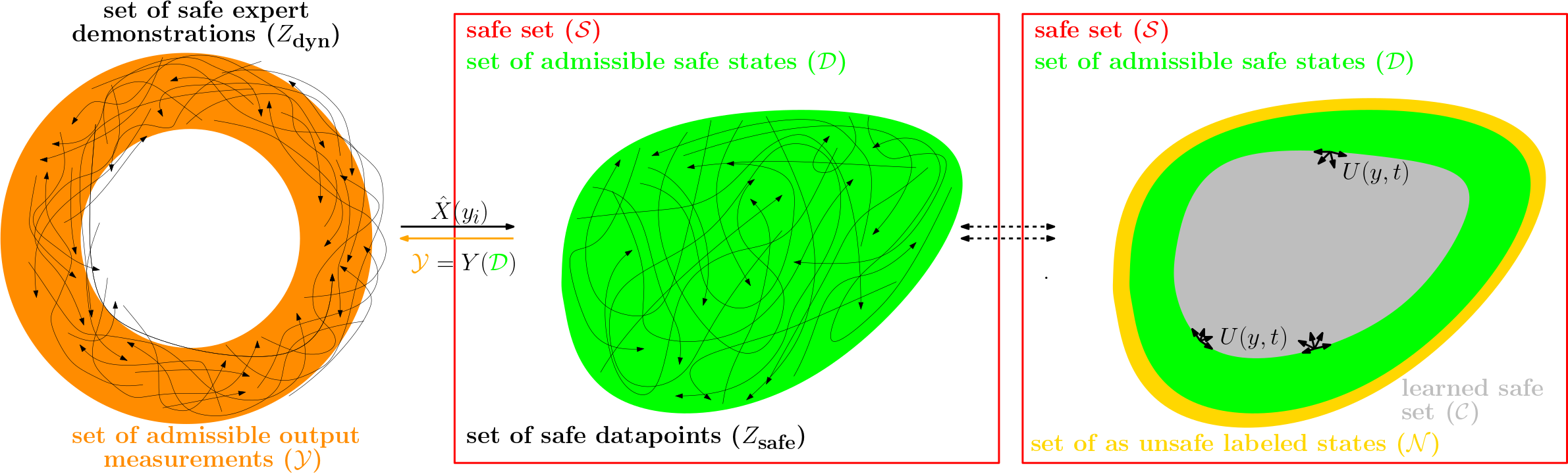
Figure 3: Problem Setup (left): The set of observed safe expert demonstrations $Z_{\mathrm{dyn}}$ (black lines). Also shown, the set of admissible output measurements $\mathcal{Y}$ (orange ring). Transformation into state domain (centre): The geometric safe set $\mathcal{S}$ (red box) and the set of admissible safe states $\mathcal{D}$ (green region) that is defined as the union of $\epsilon$-balls centered at $\hat{X}(y_{i})$. Learned safe set (right): The set of as unsafe labeled states ${\mathcal{N}}$ (golden ring) that defines the $\sigma$-layer surrounding $\mathcal{D}$.

4.2 The Constrained Optimization Problem

We first state the constrained optimization problem for learning valid ROCBFs, and then provide conditions in Section 4.3 under which a feasible solution is a valid ROCBF.

Let $\mathcal{H}$ be a normed function space of twice continuously differentiable functions $h:\mathbb{R}^{n}\to\mathbb{R}$. Define

$$q(y,t,u) :=B(\hat{X}(y),t,u)-\overline{\text{Lip}}_{B}(y,t,u)\Delta_{X}(y)$$ (6)

analogously to (4), but using a known surrogate function $\overline{\text{Lip}}_{B}(y,t,u)$ in place of the Lipschitz constant ${\text{Lip}}_{B}(y,t,u)$. The function $\overline{\text{Lip}}_{B}(y,t,u)$ will be a hyperparameter in our algorithm as discussed in Section 5, and will be adjusted to ensure that $\overline{\text{Lip}}_{B}(y,t,u)\geq{\text{Lip}}_{B}(y,t,u)$.

We formulate the following constrained optimization problem to learn a ROCBF from expert demonstrations:

$$\operatorname*{arg\!\min}_{h\in\mathcal{H}}\>\>\|h\|\>$$ (7a)

$$\mathrm{s.t.}~{}~{}h(x_{i})\geq\gamma_{\mathrm{safe}},\hskip 23.47343pt\forall x_{i}\in\underline{Z}_{\text{safe}}$$ (7b)

$$~{}~{}~{}~{}~{}~{}h(x_{i})\leq-\gamma_{\mathrm{unsafe}},\hskip 6.25963pt\forall x_{i}\in Z_{\mathcal{N}}$$ (7c)

$$~{}~{}~{}~{}~{}~{}q(y_{i},t_{i},u_{i})\geq\gamma_{\mathrm{dyn}},\forall(y_{i},t_{i},u_{i})\in Z_{\mathrm{dyn}}$$ (7d)

where the set $\underline{Z}_{\text{safe}}$ is a subset of $Z_{\text{safe}}$, i.e., $\underline{Z}_{\text{safe}}\subseteq Z_{\text{safe}}$, as detailed in the next section and where $\gamma_{\mathrm{safe}},\gamma_{\mathrm{unsafe}},\gamma_{\mathrm{dyn}}>0$ are hyperparameters. Instead of global hyperparameters $\gamma_{\mathrm{safe}}$, $\gamma_{\mathrm{unsafe}}$, and $\gamma_{\mathrm{dyn}}$, one can use individual hyperparameters for each datapoint. Note that expert demonstrations $(y_{i},t_{i},u_{i})$ indicate feasibility of the control problem at hand, and hence indicate feasibility of (7). With increasing sizes of the uncertainty sets $\mathcal{F}(x,t)$, $\mathcal{G}(x,t)$, and $\mathcal{X}(y)$, the optimization problem (7) may however become infeasible.

4.3 Conditions guaranteeing learned safe ROCBFs

We now derive conditions under which a feasible solution to the constrained optimization problem (7) is a safe ROCBF.

4.3.1 Guaranteeing $\mathcal{C}\subset\mathcal{D}\subseteq\mathcal{S}$

We begin with establishing the requirement that $\mathcal{C}\subset\mathcal{D}\subseteq\mathcal{S}$. First note that constraint (7b) ensures that the set $\mathcal{C}$, as defined in equation (5), has non-empty interior when $\underline{Z}_{\text{safe}}\neq\emptyset$. We next state conditions under which the constraint (7c) ensures that the learned function $h$ from (7) satisfies $h(x)<0$ for all $x\in{\mathcal{N}}$, which in turn ensures that $\mathcal{C}\subset\mathcal{D}\subseteq\mathcal{S}$.

Proposition 1.

Let $h(x)$ be Lipschitz continuous with local Lipschitz constant $\text{Lip}_{h}(x_{i})$ within the set $\mathcal{B}_{\epsilon_{\mathcal{N}}}(x_{i})$ for datapoints $x_{i}\in Z_{\mathcal{N}}$. Let $\gamma_{\mathrm{unsafe}}>0$, $Z_{\mathcal{N}}$ be an $\epsilon_{\mathcal{N}}$-net of ${\mathcal{N}}$, and let

$$\epsilon_{\mathcal{N}}<\frac{\gamma_{\mathrm{unsafe}}}{\text{Lip}_{h}(x_{i})}$$ (8)

for all $x_{i}\in Z_{\mathcal{N}}$. Then, the constraint (7c) ensures that $h(x)<0$ for all $x\in{\mathcal{N}}$.

In summary, Proposition 1 says that a larger Lipschitz constant of the function $h$ requires a larger margin $\gamma_{\text{unsafe}}$ and/or a finer net of unsafe datapoints as indicated by $\epsilon_{\mathcal{N}}$.

We next discuss the choice of $\underline{Z}_{\text{safe}}$. Assume first that $\underline{Z}_{\text{safe}}=Z_{\text{safe}}$ in constraint (7b). In this case, the constraints (7b) and (7c), as well as the condition in (8) of Proposition 1, may be conflicting, leading to infeasibility of the optimization problem (7). This infeasibility arises from the fact that we are simultaneously asking for the value of $h(x)$ to vary from $\gamma_{\mathrm{safe}}$ to $-\gamma_{\mathrm{unsafe}}$ over a short distance of at most $\epsilon+\epsilon_{\mathcal{N}}$ while having a small Lipschitz constant. In particular, as posed, the constraints require that $|h(x_{s})-h(x_{u})|\geq\gamma_{\mathrm{safe}}+\gamma_{\mathrm{unsafe}}$ for $x_{s}\in Z_{\mathrm{safe}}$ and $x_{u}\in Z_{\mathcal{N}}$ safe and unsafe samples, respectively, but the sampling requirements ($Z_{\mathrm{safe}}$ and $Z_{\mathcal{N}}$ being $\epsilon$ and $\epsilon_{\mathcal{N}}$-nets of $\mathcal{D}$ and $\mathcal{N}$, respectively) imply that $\|x_{s}-x_{u}\|\leq\epsilon_{\mathcal{N}}+\epsilon$ for at least some pair $(x_{s},x_{u})$, which in turn implies that

$$\text{Lip}_{h}(x_{u})\gtrsim\frac{|h(x_{s})-h(x_{u})|}{\|x_{s}-x_{u}\|}\geq\frac{\gamma_{\mathrm{safe}}+\gamma_{\mathrm{unsafe}}}{\epsilon_{\mathcal{N}}+\epsilon}.$$

The local Lipschitz constant $\text{Lip}_{h}(x_{u})$ may hence get too large if $\gamma_{\mathrm{safe}}$ and $\gamma_{\mathrm{unsafe}}$ are chosen to be too large, and we may exceed the required upper bound $\gamma_{\mathrm{unsafe}}/\epsilon_{\mathcal{N}}$ in equation (8). We address this issue as follows: for fixed $\gamma_{\mathrm{safe}}$, $\gamma_{\mathrm{unsafe}}$, and desired Lipschitz constant $L_{h}<\gamma_{\mathrm{unsafe}}/\epsilon_{\mathcal{N}}$, we define

$$\underline{Z}_{\text{safe}}:=\big{\{}x_{i}\in Z_{\mathrm{safe}}\big{|}\inf_{x\in Z_{\mathcal{N}}}\|x-x_{i}\|\geq\frac{\gamma_{\mathrm{safe}}+\gamma_{\mathrm{unsafe}}}{L_{h}}\big{\}},$$ (9)

which corresponds to a subset of admissible safe states, i.e., $\underline{Z}_{\text{safe}}\subset Z_{\text{safe}}$. Intuitively, this introduces a buffer region across which $h(x)$ can vary in value from $\gamma_{\mathrm{safe}}$ to $-\gamma_{\mathrm{unsafe}}$ for the desired Lipschitz constant $L_{h}$. Enforcing (7b) over $\underline{Z}_{\text{safe}}$ allows for smoother functions $h(x)$ to be learned at the expense of a smaller invariant safe set $\mathcal{C}$.

Note finally that, if $h(x)$ is such that $\mathcal{C}\subset\mathcal{D}$ (i.e., under the conditions in Proposition 1), then $Y(\mathcal{C})\subseteq Y(\mathcal{D})=\mathcal{Y}$ by definition of $\mathcal{Y}$ so that $\mathcal{Y}\supseteq Y(\mathcal{C})$ as required in Theorem 1.

4.3.2 Increasing the volume of $\mathcal{C}$

We next explain how to avoid learning a safe set $\mathcal{C}$ consisting of many disconnected sets, which would not be practical, and show simultaneously how to increase the volume of $\mathcal{C}$. Let

$$\underline{\mathcal{D}}:=\cup_{x_{i}\in\underline{Z}_{\text{safe}}}\mathcal{B}_{\epsilon}(x_{i})$$

and note that $\underline{Z}_{\text{safe}}$ is an $\epsilon$-net of $\underline{\mathcal{D}}$ by definition. We next show conditions under which $h(x)\geq 0$ for all $x\in\underline{\mathcal{D}}$.

Proposition 2.

Let $h(x)$ be Lipschitz continuous with local Lipschitz constant $\text{Lip}_{h}(x_{i})$ within the set $\mathcal{B}_{{\epsilon}}(x_{i})$ for datapoints $x_{i}\in\underline{Z}_{\text{safe}}$. Let $\gamma_{\text{safe}}>0$ and let

$${\epsilon}\leq\frac{\gamma_{\text{safe}}}{\text{Lip}_{h}(x_{i})}$$ (10)

for all $x_{i}\in\underline{Z}_{\text{safe}}$. Then, the constraint (7b) ensures that $h(x)\geq 0$ for all $x\in\underline{\mathcal{D}}$.

The previous result can be used to guarantee that the set $\mathcal{C}$ defined in equation (5) contains the set $\underline{\mathcal{D}}$, i.e., $\underline{\mathcal{D}}\subseteq\mathcal{C}$. Hence, the set $\underline{\mathcal{D}}$ can be seen as the minimum volume of the set $\mathcal{C}$ that we can guarantee. Note that, under the provided conditions, it holds that $\mathcal{C}$ is such that $\underline{\mathcal{D}}\subseteq\mathcal{C}\subset\mathcal{D}\subseteq\mathcal{S}$.

4.3.3 Guaranteeing that $h(x)$ is a ROCBF

Propositions 1 and 2 guarantee that the level-sets of the learned function $h(x)$ satisfy the desired geometric safety properties. We now derive conditions that ensure that $h(x)$ is a ROCBF, i.e., that the ROCBF constraint (4) is also satisfied.

To satisfy constraint (4) for each $(y,t)\in\mathcal{Y}\times\mathbb{R}_{\geq 0}$, there must exist a control input $u\in\mathcal{U}$ such that $q(y,t,u)\geq 0$. We follow a similar idea as in Propositions 1 and 2 and note in this respect that the $y$ components of $Z_{\mathrm{dyn}}$ form an $\bar{\epsilon}$-net of $\mathcal{Y}$ (see Appendix D for a proof) where $\bar{\epsilon}$ is

$$\bar{\epsilon}:=\text{Lip}_{Y}(\epsilon+\bar{\Delta}_{X})$$

with $\bar{\Delta}_{X}:=\sup_{y\in\mathcal{Y}}\Delta_{X}(y)$ denoting the maximum estimation error and $\text{Lip}_{Y}$ being the Lipschitz constant of the output measurement map $Y$ within the set $\overline{\mathcal{D}}:=\mathcal{D}\oplus\mathcal{B}_{2\bar{\Delta}_{X}}(0)$.

We additionally assume to know a bound on the difference of the function $q$ for different times $t$. More formally, for each $\bar{y}\in\mathcal{B}_{\bar{\epsilon}}(y)$, let $\text{Bnd}_{q}(y,u)$ be such that

$$|q(\bar{y},t^{\prime},u)-q(\bar{y},t^{\prime\prime},u)|\leq\text{Bnd}_{q}(y,u),\forall t^{\prime},t^{\prime\prime}\geq 0.$$ (11)

The bound $\text{Bnd}_{q}(y,u)$ exists and can be obtained as all components of $q(y,t,u)$ are bounded in $t$. This is a natural assumption to obtain formal guarantees on the function $q(y,t,u)$ from a finite dataset $Z_{\text{dyn}}$ since it is not possible to sample the time domain $\mathbb{R}_{\geq 0}$ densely with a finite number of samples. It can be seen that $\text{Bnd}_{q}(y,u)=0$ when the system (1) is independent of $t$.

Proposition 3.

Let $q(y,t,u)$ be Lipschitz continuous in $y$ for fixed $t$ and $u$ with local Lipschitz constant $\text{Lip}_{q}(y_{i},t_{i},u_{i})$ within the set $\mathcal{B}_{\bar{\epsilon}}(y_{i})$ for each $(y_{i},t_{i},u_{i})\in Z_{\text{dyn}}$. Let $\gamma_{\text{dyn}}>0$ and

$$\bar{\epsilon}\leq\frac{\gamma_{\text{dyn}}-\text{Bnd}_{q}(y_{i},u_{i})}{\text{Lip}_{q}(y_{i},t_{i},u_{i})}$$ (12)

for all $(y_{i},t_{i},u_{i})\in Z_{\text{dyn}}$. Then, the constraint (7d) ensures that, for each $(y,t)\in\mathcal{Y}\times\mathbb{R}_{\geq 0}$, there exists a $u\in\mathcal{U}$ such that $q(y,t,u)\geq 0$. If additionally ${\text{Lip}}_{B}(y,t,u)\leq\overline{\text{Lip}}_{B}(y,t,u)$ for each $(y,t,u)\in\mathcal{Y}\times\mathbb{R}_{\geq 0}\times\mathcal{U}$, then $h(x)$ is a ROCBF.

In summary, Proposition 3 says that a larger Lipschitz constant of the function $q$ requires a larger margin $\gamma_{\text{dyn}}$ and/or a smaller $\bar{\epsilon}$, i.e., a finer net of safe datapoints as indicated by $\epsilon$ and/or a reduction in the measurement map error $\Delta_{X}$.

The next theorem summarizes our results, follows from the previous results, and is provided without proof.

Theorem 2.

Let $h(x)$ be a twice continuously differentiable function. Let the sets $\mathcal{S}$, $\mathcal{C}$, $\mathcal{Y}$, $\underline{\mathcal{D}}$, and ${\mathcal{N}}$ as well as the data-sets $\underline{Z}_{\text{safe}}$, $Z_{\mathrm{dyn}}$, and $Z_{\mathcal{N}}$ be defined as above. Suppose that $Z_{\mathcal{N}}$ forms an $\epsilon$-net of ${\mathcal{N}}$ and that the conditions (8), (10), and (12) are satisfied. Assume also that ${\text{Lip}}_{B}(y,t,u)\leq\overline{\text{Lip}}_{B}(y,t,u)$ for each $(y,t,u)\in\mathcal{Y}\times\mathbb{R}_{\geq 0}\times\mathcal{U}$. If $h(x)$ satisfies the constraints (7b), (7c), and (7d), then $h(x)$ is a ROCBF on $\mathcal{Y}$ and it holds that the set $\mathcal{C}$ is non-empty and such that $\underline{\mathcal{D}}\subseteq\mathcal{C}\subseteq\mathcal{S}$.

5 Algorithmic Implementation

In this section, we present the algorithmic implementation of the previously presented results. We will discuss various aspects related to solving the constrained optimization problem (7), the construction of the involved datasets, and estimating Lipschitz constants of the functions $h(x)$ and $q(y,t,u)$.

5.1 The Algorithm

We summarize our algorithm to learn safe ROCBFs $h(x)$ in Algorithm 1. We first construct the set of safe datapoints $Z_{\text{safe}}$ from the expert demonstrations $Z_{\text{dyn}}$ (line 3). We construct the set of as unsafe labeled datapoints $Z_{\mathcal{N}}$ from $Z_{\text{safe}}$ (line 4), i.e., $Z_{\mathcal{N}}\subseteq Z_{\text{safe}}$, by identifying boundary points in $Z_{\text{safe}}$ and labeling them as unsafe (details can be found in Section 5.5.2). We then re-define $Z_{\text{safe}}$ by removing the unsafe labeled datapoints $Z_{\mathcal{N}}$ from $Z_{\text{safe}}$ (line 5). Following our discussion in Section 4.4.3, we obtain $\underline{Z}_{\text{safe}}$ according to equation (9) (line 6). We then solve the constrained optimization problem (7) by an unconstrained relaxation defined in (13) (line 7) as discussed in Section 5.5.3. Finally, we check if the constraints (7b)-(7d) and the constraints (8), (10), (12) are satisfied by the learned function $h(x)$ (line 8). If the constraints are not satisfied, the hyperparameters are adjusted and the process is repeated (line 9). We discuss Lipschitz constant estimation of $h$ and $q$ and the hyperparameter selection in Section 5.5.4.

1:Input: Set of expert demonstrations $Z_{\text{dyn}}$,

2:system model $(\hat{F},\hat{G},\hat{X},\Delta_{F},\Delta_{G},\Delta_{X})$,

3:hyperparameters $(\alpha,\gamma_{\text{safe}},\gamma_{\text{unsafe}},\gamma_{\text{dyn}},L_{h},\overline{\text{Lip}}_{B},k,\eta)$

4:Output: Safe ROCBF $h(x)$

5:$Z_{\text{safe}}\leftarrow\cup_{(y_{i},t_{i},u_{i})\in Z_{\text{dyn}}}\hat{X}(y_{i})$  # Safe datapoints

6:$Z_{\mathcal{N}}\leftarrow\textsc{BPD}(Z_{\text{safe}},k,\eta)$  # Unsafe datapoints obtained by boundary point detection (BPD) in Algorithm 2.

7:$Z_{\text{safe}}\leftarrow Z_{\text{safe}}\setminus Z_{\mathcal{N}}$

8:$\underline{Z}_{\text{safe}}\leftarrow$ according to (9)

9:$h(x)\leftarrow$ solution of (13)  # relaxation of the constrained optimization problem in (7)

10:while constr. (7b)-(7d), (8), (10), (12) are violated do

11:   Modify hyperparameters and start from line 3

12:end while

Algorithm 1 Learning ROCBF from Expert Demonstrations

While our algorithmic implementation is an approximate solution of the proposed framework, we mention that solving an unconstrained relaxation of (7) and bootstrapping hyperparameters is a common technique in machine learning when solving nonconvex constrained optimization problems [56]. Such techniques are necessary for learning based methods to be applied to realistic systems. As we reported in earlier works, see e.g., [49] for hybrid systems, such techniques perform well in practice and can even outperform experts.

5.2 Construction of the Datasets

Due to the conditions in equations (8), (10), and (12), the first requirement is that the datasets $\underline{Z}_{\text{safe}}$ and $Z_{\mathcal{N}}$ are dense, i.e., that $\epsilon$ and $\epsilon_{\mathcal{N}}$ are small. It is also required that $Z_{\mathcal{N}}$ is an $\epsilon_{\mathcal{N}}$-net of the set of unsafe labeled states $\mathcal{N}$. In order to construct the $\epsilon_{\mathcal{N}}$-net $Z_{\mathcal{N}}$ of $\mathcal{N}$, a simple randomized algorithm, which repeatedly uniformly samples from $\mathcal{N}$, works with high probability, see e.g., [57]. Hence, as long as we can efficiently sample from $\mathcal{N}$, e.g., when $\mathcal{N}$ is a basic primitive set or has a set-membership oracle, uniform sampling or gridding methods are viable strategies.

However, as this is in general not possible, we use a boundary point detection algorithm in line 4 of Algorithm 1. The idea is to obtain the set of unsafe labeled datapoints $Z_{\mathcal{N}}$ instead from the set of safe datapoints $Z_{\text{safe}}$. To perform this step efficiently, our approach is to detect geometric boundary points of the set $Z_{\mathrm{safe}}$. This subset of boundary points is labeled as $Z_{\mathcal{N}}$, while we re-define $Z_{\mathrm{safe}}$ to exclude the boundary points $Z_{\mathcal{N}}$ in line 5 of Algorithm 1. Particularly, we detect boundary points in $Z_{\mathrm{safe}}$ based on the concept of reverse $k$-nearest neighbors, see e.g., [58]. The main idea is that boundary points typically have fewer reverse $k$-nearest neighbors than interior points. For $k>0$, we find the $k$-nearest neighbors of each datapoint $x_{i}\in Z_{\mathrm{safe}}$. Then, we find the reverse $k$-nearest neighbors of each datapoint $x_{i}\in Z_{\mathrm{safe}}$, that is, we find the datapoints $x_{i}^{\prime}\in Z_{\mathrm{safe}}$ that have $x_{i}$ as their $k$-nearest neighbor. Finally, we choose a threshold $\eta>0$ and label all datapoints $x_{i}\in Z_{\mathrm{safe}}$ as a boundary point whose cardinality of reverse $k$-nearest neighbors is below $\eta$.

Algorithm 2 summarizes the boundary point detection algorithm. We first compute the pairwise distances between each of the $N_{1}$ safe datapoints in $Z_{\text{safe}}$ (line 1). The result is a symmetric $N_{1}\times N_{1}$ matrix $M$ where the element at position $(i,j)$ represents the pairwise distance between the states $x_{i}$ and $x_{j}$, i.e., $M_{ij}:=\|x_{i}-x_{j}\|$. Next, we calculate the $k$-nearest neighbors of each $x_{i}$, denoted by $kNN_{i}$, as the set of indices corresponding to the $k$ smallest column entries in the $i$th row of $M$ (line 2). We calculate the reverse $k$-nearest neighbors of each $x_{i}$ as $RkNN_{i}:=|\{x_{j}\in Z_{\mathrm{safe}}|x_{i}\in kNN_{j}\}|$ (line 3). We then threshold each $RkNN_{i}$ by $\eta$ (line 4), i.e., $z_{i}:=\mathbbm{1}(RkNN_{i}\leq\eta)$ where $\mathbbm{1}$ is the indicator function. We obtain a tuple $(z_{1},\ldots,z_{N_{1}})\in\mathbb{R}^{N_{1}}$, where the indices $i$ corresponding to states $x_{i}=1$ are boundary points.

1:Input: Set of safe states $Z_{\text{safe}}$, number of nearest neighbors $k$, neighbor threshold $\eta>0$

2:Output: Set of boundary points, i.e., the set of as unsafe labeled states $Z_{\mathcal{N}}$

3:$M\leftarrow compute\_pairwise\_dists(Z_{\text{safe}})$  # compute pairwise distances between elements in $Z_{\text{safe}}$

4:$kNN_{i}\leftarrow compute\_k\_nearest\_neighbors(M)$  # compute $k$-nearest neighbors of $x_{i}\in Z_{\mathrm{safe}}$

5:$RkNN_{i}\leftarrow compute\_reverse\_k\_nearest\_neighbors(kNN)$  # compute reverse $k$-nearest neighbors of $x_{i}\in Z_{\mathrm{safe}}$

6:$z_{i}\leftarrow\mathbbm{1}(RkNN_{i}\leq\eta)$  # threshold $RkNN_{i}$ by $\eta$

Algorithm 2 Boundary Point Detection - BPD($Z_{\text{safe}}$,$k$,$\eta$)

We have not yet specified the paramters $\epsilon$ and $\epsilon_{\mathcal{N}}$ to be able to check the constraints (8), (10), and (12). While the value of $\epsilon$ merely defines the set of admissible states $\mathcal{D}$ and determines the size of the safe set $\mathcal{C}$ as discussed in Section 4.4.3, the value of $\epsilon_{\mathcal{N}}$ is important as the set of unsafe labeled states $\mathcal{N}$ should fully enclose $\mathcal{D}$. This imposes an implicit lower bound on $\epsilon_{\mathcal{N}}$ to guarantee safety. Therefore, one can artificially sample additional datapoints in proximity of $Z_{\mathcal{N}}$ and add these to the set $Z_{\mathcal{N}}$. One way to get an estimate of $\epsilon_{\mathcal{N}}$ is to calculate the distance of each datapoint to the closest datapoint in $Z_{\mathcal{N}}$, respectively. Then, taking the maximum or an average over these values gives a good estimate of $\epsilon_{\mathcal{N}}$.

Finally, we discuss what behavior expert demonstrations in $Z_{\mathrm{dyn}}$ should exhibit. We focus on the ROCBF constraint (4), which must be verified to hold for some $u\in\mathcal{U}$, by using the expert demonstration $(y_{i},t_{i},u_{i})$ in (7d). The more transverse the vector field of the input dynamics $\langle\hat{G}(\hat{X}(y_{i}),t_{i}),u_{i}\rangle$ is to the level sets of the function $h(\hat{X}(y_{i}))$ (i.e., the more parallel it is to the inward pointing normal $\nabla h(\hat{X}(y_{i}))$), the larger the inner-product term in constraint (7d) will be without increasing the Lipschitz constant of $h(x)$. This means that the expert demonstrations should demonstrate how to move away from the unsafe labeled set.

5.3 Solving the Constrained Optimization Problem

Some remarks are in order with respect to the optimization problem (7). If the extended class $\mathcal{K}$ function $\alpha$ is linear and $\mathcal{H}$ is parameterized as $\mathcal{H}:=\{\langle\phi(x),\theta\rangle|\theta\in\Theta\}$ where $\Theta\subseteq\mathbb{R}^{l}$ is a convex set and $\phi:\mathbb{R}^{n}\to\mathbb{R}^{l}$ is a known basis function, then the optimization problem (7) is convex. Note here in particular that $\|\nabla h(x)\|_{\star}$ is convex in $\theta$ since 1) $\nabla h(x)$ is linear in $\theta$, 2) norms are convex functions, and 3) composition of a convex with a linear function preserves convexity. We remark that rich function classes such as infinite dimensional reproducing kernel Hilbert spaces can be approximated to arbitrary accuracy with such an $\mathcal{H}$ [59].

In the more general case when $\mathcal{H}:=\{h(x;\theta)|\theta\in\Theta\}$, such as when $h(x;\theta)$ is a deep neural network or when $\alpha$ is a general nonlinear function, the optimization problem (7) is nonconvex. Due to the computational complexity of general nonlinear constrained programming, we propose an unconstrained relaxation of the optimization problem (7). Our unconstrained relaxation results in the optimization problem:

$$\max_{\lambda_{\mathrm{s}},\lambda_{\mathrm{u}},\lambda_{\mathrm{d}}} \min_{\theta\in\Theta}\|\theta\|^{2}+\lambda_{\mathrm{s}}\sum_{x_{i}\in\underline{Z}_{\text{safe}}}\Big{[}\gamma_{\mathrm{safe}}-h(x_{i};\theta)\Big{]}_{+}$$ (13a)

$$+\lambda_{\mathrm{u}}\sum_{x_{i}\in Z_{\mathcal{N}}}\Big{[}h(x_{i};\theta)+\gamma_{\mathrm{unsafe}}\Big{]}_{+}$$ (13b)

$$+\lambda_{\mathrm{d}}\sum_{(y_{i},t_{i},u_{i})\in Z_{\mathrm{dyn}}}\Big{[}\gamma_{\mathrm{dyn}}-q(y_{i},t_{i},u_{i};\theta)\Big{]}_{+}$$ (13c)

where $[r]_{+}:=\max\{r,0\}$ for $r\in\mathbb{R}$ and where the function $q(u,y,t;\theta)$ is as in (6) but now defined via $h(x;\theta)$. The positive parameters $\lambda_{\mathrm{s}}$, $\lambda_{\mathrm{u}}$, and $\lambda_{\mathrm{d}}$ are dual variables. While the unconstrained optimization problem (13) is in general a nonconvex optimization problem, it can be solved efficiently in practice by iteratively solving the outer and inner optimization problems with respect to $(\lambda_{\mathrm{s}},\lambda_{\mathrm{u}},\lambda_{\mathrm{d}})$ and $\theta$, respectively, with stochastic first-order gradient methods such as Adam or stochastic gradient descent [56].

5.4 Hyperparameter Selection and Lipschitz constant Estimation

We treat $(\alpha,\gamma_{\text{safe}},\gamma_{\text{unsafe}},\gamma_{\text{dyn}},L_{h},\overline{\text{Lip}}_{B},k,\eta)$ as hyperparameters and bootstrap over them. This is a common technique in machine learning and usually done via grid search. Due to the nonconvexity of the optimization problem, one may not be able to satisfy all constraints in (7b)-(7d), (8), (10), (12). We hence terminate the while loop in line 9 of Algorithm 1 when a satisfactory empirical behavior is achieved.

The conditions in equations (8), (10), and (12) depend on Lipschitz constants of the functions $h$ and $q$. Since we assume that $h$ is twice continuously differentiable and we restrict ourselves to a compact domain ${\mathcal{N}}\cup\mathcal{D}$, we have that $h$ and $\nabla h$ are both uniformly Lipschitz over ${\mathcal{N}}\cup\mathcal{D}$. In [48], we showed two examples of $\mathcal{H}$ (we considered DNNs and functions parametrized by random Fourier features) where an upper bound on the Lipschitz constants of functions $h\in\mathcal{H}$ and its gradient $\nabla h(x)$ can be efficiently estimated, and we refer the interested reader to [48].

6 Simulations

(a) Training course.

(b) Test course.

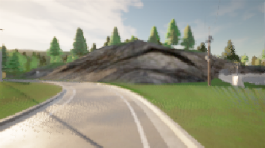
(c) Downsampled camera image.

Figure 4: Simulation environment in CARLA. The cars are tracking desired reference paths on different courses. Left: The training course from which training data, during a left turn, was generated to train and test the ROCBF. Middle: An unknown test course on which the learned ROCBF is tested. Right: Downsampled RGB dashboard camera image.

We construct a safe ROCBF within the autonomous driving simulator CARLA [51] for a car driving on a highway by using camera images, see Fig. 4. In particular, our goal is to learn a ROCBF for the lateral control of the car, i.e., a lane keeping controller, while we use a built-in controller for longitudinal control. Lane keeping in CARLA is achieved by tracking a set of predefined waypoints. The control problem at hand is challenging which makes it difficult to satisfy all constraints in equations (7b)-(7d) and (8), (10), (12). As described in Section 5.5.4, we search over the hyperparameters of Algorithm 1 until satisfactory behavior is achieved. The code for our simulations and videos of the car under the learned safe ROCBFs are available at

https://github.com/unstable-zeros/learning-rocbfs.

As we have no direct access to the system dynamics of the car, we identify a system model. The model for longitudinal control is estimated from data and consists of the velocity $v$ of the car and the integrator state $d$ of the PID. The identified longitudinal model of the car is

$$\dot{v} =-1.0954v-0.007v^{2}-0.1521d+3.7387$$

$$\dot{d} =3.6v-20.$$

For the lateral control of the car, we consider a bicycle model

$$\dot{p}_{x} =v\cos(\theta),$$

$$\dot{p}_{y} =v\sin(\theta),$$

$$\dot{\theta} =v/L\tan(\delta),$$

where $p_{x}$ and $p_{y}$ denote the position in a global coordinate frame, $\theta$ is the heading angle with respect to a global coordinate frame, and $L:=2.51$ is the distance between the front and the rear axles of the car. The control input is the steering angle $\delta$ that we design such that the car tracks waypoints provided by CARLA. Treating $u:=\tan(\delta)$ as the control input yields a control affine system.

To be able to learn a ROCBF in a data efficient manner, we convert the above lateral model (defined in a global coordinate frame) into a local coordinate frame. We do so relatively to the waypoints that the car has to follow. We consider the cross-track error $c_{e}$ of the car. In particular, let $wp_{1}$ be the waypoint that is closest to the car and let $wp_{2}$ be the waypoint proceeding $wp_{1}$. Then the cross-track error is defined as $c_{e}:=\|w\|\sin(\theta_{w})$ where $w\in\mathbb{R}^{2}$ is the vector pointing from $wp_{1}$ to the car and $\theta_{w}$ is the angle between $w$ and the vector pointing from $wp_{1}$ to $wp_{2}$. We further consider the error angle $\theta_{e}:=\theta-\theta_{t}$ where $\theta_{t}$ is the angle between the vector pointing from $wp_{1}$ to $wp_{2}$ and the global coordinate frame. The simplified local model is

$$\dot{c}_{e} =v\sin(\theta_{e}),$$

$$\dot{\theta}_{e} =v/2.51u-\dot{\theta}_{t}.$$

In summary, we have the state $x:=\begin{bmatrix}v&d&c_{e}&\theta_{e}\end{bmatrix}^{T}$ and the control input $u:=\tan(\delta)$ as well as the external input, given during runtime, of $\dot{\theta}_{t}$. Consequently, let

$$\hat{F}:=\begin{bmatrix}-1.095v-0.007v^{2}-0.152d+3.74\\ 3.6v-20\\ v\sin(\theta_{e})\\ -\dot{\theta}_{t}\end{bmatrix}\hat{G}:=\begin{bmatrix}0\\ 0\\ 0\\ v/2.51\end{bmatrix}$$

along with estimated error bounds $\Delta_{F}(x,t):=0.1$ and $\Delta_{G}(x,t)=0.1$ (calculated from simulations).

For collecting safe expert demonstrations $Z_{\text{dyn}}$, we use an “expert” PID controller $u(x)$ that uses full state knowledge of $x$. Throughout this section, we use the parameters $\alpha(r):=r$, $\gamma_{\text{safe}}:=\gamma_{\text{unsafe}}:=0.05$, and $\gamma_{\text{dyn}}:=0.01$ to train safe ROCBFs $h(x)$. For the boundary point detection algorithm in Algorithm 2, we select $k:=200$ and $\eta$ such that $40$ percent of the points in $Z_{\text{safe}}$ are labeled as boundary points.

6.1 State-based ROCBF

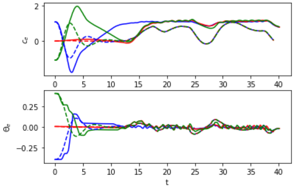
(a) Trajectories $c_{e}(t)$ and $\theta_{e}(t)$ for different initial conditions indicated by color. Solid lines correspond to the learned ROCBF, while dashed lines correspond to the expert (PID).

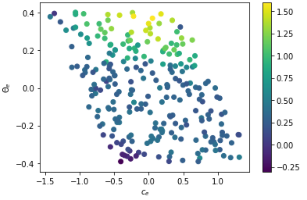
(b) Shown are 250 different initial conditions on the training course. The color legend encodes $\max_{t}|c_{e}^{ROCBF}(t)|-\max_{t}|c_{e}^{Exp}(t)|$.

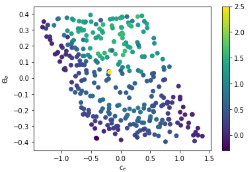
(c) Shown are 300 different initial conditions on the test course. The color legend encodes $\max_{t}|c_{e}^{ROCBF}(t)|-\max_{t}|c_{e}^{Exp}(t)|$.

Figure 5: State-based ROCBF controller.

We first learn a ROCBF controller in the case that the state $x$ is perfectly known, i.e., the model of the output measurement map is such that $\hat{X}(y)=X(y)=x$ and the error is $\Delta_{X}(y):=0$. The trained ROCBF $h(x)$ is a two-layer DNN with 32 and 16 neurons per layer.

The safety controller applied to the car is then obtained as the solution of the convex optimization problem $\min_{u\in\mathcal{U}}\|u\|$ subject to the constraint $q(u,y,t)\geq 0$. In Fig. 5(a), example trajectories of $c_{e}(t)$ and $\theta_{e}(t)$ under this controller are shown. Solid lines indicate the learned ROCBF controller, while dashed lines indicate the expert PID controller for comparison. Colors in both subplots match the corresponding trajectories. The initial conditions of $d(0)$ and $v(0)$ are set to zero in all cases here, similar to all other plots in the remainder. Fig. 5(b) shows different initial conditions $c_{e}(0)$ and $\theta_{e}(0)$ and how the ROCBF controller performs relatively to the expert PID controller on the training course. In particular, each point in the plot indicates an initial condition from which system trajectories under both the ROCBF and expert PID controller are collected. The color map shows

$$\max_{t}|c_{e}^{ROCBF}(t)|-\max_{t}|c_{e}^{Exp}(t)|$$

where $c_{e}^{ROCBF}(t)$ and $c_{e}^{Exp}(t)$ denote the cross-track errors under the ROCBF and expert PID controllers, respectively. Fig. 5(c) shows the same plot, but for the test course from which no data has been collected to train the ROCBF. In this plot, one ROCBF trajectory resulted in a collision as detected by CARLA. We assign by default a value of $2.5$ in case of a collision (see the yellow point in Fig. 5(c)).

6.2 Perception-based ROCBF

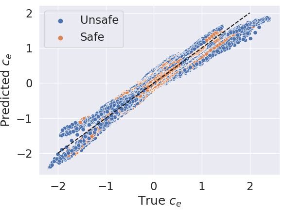
(a) Performance of the perception map $\hat{X}$ on training data. Blue and orange are boundary and non-boundary points from Algorithm 2.

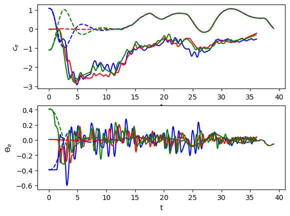
(b) Trajectories $c_{e}(t)$ and $\theta_{e}(t)$ for different initial conditions indicated by color. Solid lines correspond to the learned ROCBF, while dashed lines correspond to the expert (PID).

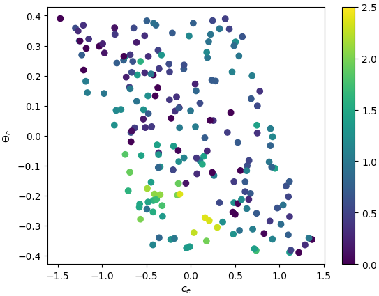
(c) Shown are 200 different initial conditions on the training course. The color legend encodes $\max_{t}|c_{e}^{ROCBF}(t)|-\max_{t}|c_{e}^{Exp}(t)|$.

Figure 6: Perception-based ROCBF controller.

We next learn a ROCBF in the case that $y$ corresponds to images taken from an RGB camera mounted to the dashboard of the car. To train a perception map $\hat{X}$, we have resized the images as shown in Fig. 4(c). We assume knowledge of $\theta_{e}$, $v$, and $d$, while we estimate $c_{e}$ from $y$, i.e., $x:=\begin{bmatrix}v&d&\hat{X}(y)&\theta_{e}\end{bmatrix}^{T}$. The architecture of $\hat{X}$ is a Resnet18, i.e., a convolutional neural network with 18 layers. Its performance on training data within operation range $c_{e}\in[-2,2]$ is shown in Fig. 6(a). Based on this plot, we set $\Delta_{X}(y):=0.5$ to account for estimation errors within this range. We remark that we observed larger estimation errors outside this range. However, larger $\Delta_{X}(y)$ resulted in learning infeasible ROCBFs. We additionally selected the hyperparameter $\overline{\text{Lip}}_{B}(y,t,u):=\overline{\text{Lip}}_{1}+\overline{\text{Lip}}_{2}\|u\|$. We achieved the best results by using $\overline{\text{Lip}}_{1}=\overline{\text{Lip}}_{2}:=0.1$ during testing, while using the norm of the partial derivatives of $\langle\nabla h(x),\hat{F}(x,t)\rangle+\alpha(h(x))-\|\nabla h(x)\|_{2}\Delta_{F}(x,t)$ and $\langle\nabla h(x),\hat{G}(x,t)\rangle-\|\nabla\|_{2}\Delta_{G}(x,t)$, respectively, during training. The trained ROCBF $h(x)$ is again a two-layer DNN with 32 and 16 neurons per layer. Figs. 6(b)-6(c) show the same plots as in the previous section and evaluate the ROCBF relatively to the expert PID controller. Importantly, note here that the expert PID controller uses state knowledge, while the ROCBF uses RGB images from the dashboard camera as inputs so that it is no surprise that the relative gap between these two, as shown in Figs. 6(c) and 6(c), becomes larger.

In Fig. 7, we further illustrate the level sets of the learned function $h(x)$ within the $c_{e}$-$\theta_{e}$ plane for fixed values of $v$ and $d$. Note that a visualization of the level sets in four dimensions is in general difficult.

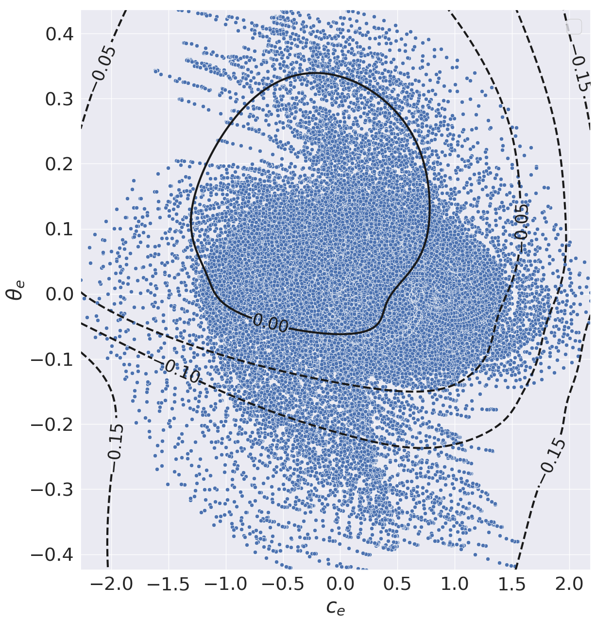
Figure 7: Illustration of the level sets of the learned function $h(x)$ in the $c_{e}$-$\theta_{e}$ plane for fixed values of $v$ and $d$ for the perception-based ROCBF. The plot also shows all training datapoints projected onto the $c_{e}$-$\theta_{e}$ plane.

7 Conclusion and Summary

In this paper, we have shown how safe control laws can be learned from expert demonstrations under system model and measurement map uncertainties. We first presented robust output control barrier functions (ROCBFs) as a means to enforce safety, which is here defined as the ability of a system to remain within a safe set using the notion of forward invariance. We then proposed an optimization problem to learn such ROCBFs from safe expert demonstrations, and presented verifiable conditions for the validity of the ROCBF. These conditions are stated in terms of the density of the data and on Lipschitz and boundedness constants of the learned function as well as the models of the system dynamics and the measurement map. We proposed an algorithmic implementation of our theoretical framework to learn ROCBFs in practice. Finally, our simulation studies show how to learn safe control laws from RGB camera images within the autonomous driving simulator CARLA.

Appendix

Appendix A Proof of Theorem 1

Recall that $f(t):=F(x(t),t)$, $g(t):=G(x(t),t)$, $y(t):=Y(x(t))$ and $u(t):=U(y(t),t)$ according to (1c)-(1f) and we define for convenience

$$\hat{f}(t) :=\hat{F}(x(t),t)$$

$$\hat{g}(t) :=\hat{G}(x(t),t)$$

$$\delta_{F}(t) :=\Delta_{F}(x(t),t)$$

$$\delta_{G}(t) :=\Delta_{G}(x(t),t)$$

$$\hat{x}(t) :=\hat{X}(y(t)).$$

Due to the chain rule and since $U(y,t)\in\mathcal{U}_{\text{s}}(y,t)$, note that each solution $x:\mathcal{I}\to\mathbb{R}^{n}$ to (1) under $U(y,t)$ satisfies

$$\begin{split}B(\hat{x}(t),t,u(t))\geq\text{Lip}_{B}(y(t),t,u(t))\Delta_{X}(y(t)).\end{split}$$ (14)

Note now that the term $\text{Lip}_{B}(y(t),t,u(t))\Delta_{X}(y(t))$ in the right-hand side of (14) can be bounded as

$$\text{Lip}_{B}(y(t),t,u(t))\Delta_{X}(y(t))$$

$$\overset{(a)}{\geq} \text{Lip}_{B}(y(t),t,u(t))\|\hat{x}(t)-x(t)\|$$

$$\overset{(b)}{\geq} |B(\hat{x}(t),t,u(t))-B(x(t),t,u(t))|$$

$$\geq B(\hat{x}(t),t,u(t))-B(x(t),t,u(t))$$

where $(a)$ follows since $x(t)\in\mathcal{X}(y(t))$ due to Assumption 2 and where $(b)$ simply follows since $\text{Lip}_{B}(y(t),t,u(t))$ is the local Lipschitz constant of the function $B(x,t,u)$ within the set $\mathcal{X}(y(t))$. From (14) and the definitions of the functions $B(x,t,u)$ and $\text{Lip}_{B}(y,t,u)$, it hence follows that $B(x(t),t,u(t))\geq 0$. Note next that the following holds

$$B(x(t),t,u(t))\geq 0$$

$$\Leftrightarrow \langle\nabla h(x(t)),\hat{f}(t)+\hat{g}(t)u(t)\rangle+\alpha(h(x(t)))$$

$$\geq\|\nabla h(x(t))\|_{\star}(\delta_{F}(t)+\delta_{G}(t)\|u(t)\|)$$

$$\overset{(c)}{\Rightarrow} \langle\nabla h(x(t)),f(t)+g(t)u(t)\rangle+\alpha(h(x(t)))\geq 0$$

$$\Leftrightarrow \dot{h}(x(t))\geq-\alpha(h(x(t)))$$ (15)

where the implication in $(c)$ follows since

$$\|\nabla h(x(t))\|_{\star}(\delta_{F}(t)+\delta_{G}(t)\|u(t)\|)$$

$$\overset{(d)}{\geq} \|\nabla h(x(t))\|_{\star}(\|\hat{f}(t)-f(t)\|+{|\kern-1.07639pt|\kern-1.07639pt|\hat{g}(t)-g(t)|\kern-1.07639pt|\kern-1.07639pt|}\|u(t)\|)$$

$$\overset{(e)}{\geq} \|\nabla h(x(t))\|_{\star}(\|\hat{f}(t)-f(t)\|+\|(\hat{g}(t)-g(t))u(t))\|)$$

$$\overset{(f)}{\geq} \langle\nabla h(x(t)),\hat{f}(t)+\hat{g}(t)u(t)\rangle-\langle\nabla h(x(t)),{f}(t)+{g}(t)u(t)\rangle$$

where the inequality $(d)$ follows since $f(t)\in\mathcal{F}(x(t),t)$ and $g(t)\in\mathcal{G}(x(t),t)$ due to Assumption 1 and where the inequality $(e)$ follows by properties of the induced matrix norm ${|\kern-1.07639pt|\kern-1.07639pt|\cdot|\kern-1.07639pt|\kern-1.07639pt|}$. The inequality $(f)$ follows by application of Hölder’s inequality. Consequently, by (15) it holds that $\dot{h}(x(t))\geq-\alpha(h(x(t)))$ for all $t\in\mathcal{I}$.

Next note that $\dot{v}(t)=-\alpha(v(t))$ with $v(0)\geq 0$ admits a unique solution $v(t)$ that is such that $v(t)\geq 0$ for all $t\geq 0$ [60, Lemma 4.4]. Using the Comparison Lemma [60, Lemma 3.4] and assuming that $h(x(0))\geq 0$, it follows that $h(x(t))\geq v(t)\geq 0$ for all $t\in\mathcal{I}$, i.e., $x(0)\in\mathcal{C}$ implies $x(t)\in\mathcal{C}$ for all $t\in\mathcal{I}$. Recall next that (1) is defined on $X(\mathcal{Y})$ and that $\mathcal{Y}\supseteq Y(\mathcal{C})$ and hence $X(\mathcal{Y})\supseteq\mathcal{C}$ holds. Since $x\in\mathcal{C}$ for all $t\in\mathcal{I}$ and when $\mathcal{C}$ is compact, it follows by [60, Theorem 3.3] that $\mathcal{I}=[0,\infty)$, i.e., $\mathcal{C}$ is forward invariant under $U(y,t)$.

Appendix B Proof of Proposition 1

Note first that, for any $x\in{\mathcal{N}}$, there exists a point $x_{i}\in Z_{\mathcal{N}}$ satisfying $\|x-x_{i}\|\leq\epsilon_{\mathcal{N}}$ since $Z_{\mathcal{N}}$ is an $\epsilon_{\mathcal{N}}$-net of ${\mathcal{N}}$. For any $x\in{\mathcal{N}}$, we now select such an $x_{i}\in Z_{\mathcal{N}}$ for which it follows that

$$h(x)=h(x)-h(x_{i})+h(x_{i})\overset{(a)}{\leq}|h(x)-h(x_{i})|-\gamma_{\mathrm{unsafe}}$$

$$\overset{(b)}{\leq}\text{Lip}_{h}(x_{i})\|x-x_{i}\|-\gamma_{\mathrm{unsafe}}\overset{(c)}{\leq}\text{Lip}_{h}(x_{i})\epsilon_{\mathcal{N}}-\gamma_{\mathrm{unsafe}}\overset{(d)}{<}0.$$

Note that inequality $(a)$ follows from constraint (7c), while inequality $(b)$ follows by Lipschitz continuity. Inequality $(c)$ follows by the assumption of $Z_{\mathcal{N}}$ being an $\epsilon_{\mathcal{N}}$-net of ${\mathcal{N}}$ and, finally, the strict inequality in $(d)$ follows due to (8).

Appendix C Proof of Proposition 2

The proof follows similarly to the proof of Proposition 1. For any $x\in\underline{\mathcal{D}}$, we select an $x_{i}\in\underline{Z}_{\text{safe}}$ with $\|x-x_{i}\|\leq{\epsilon}$ which is possible since the set $\underline{Z}_{\text{safe}}$ is an ${\epsilon}$-net of $\underline{\mathcal{D}}$. It follows that

$$0=h(x_{i})-h(x_{i}) \overset{(a)}{\leq}h(x_{i})-h(x)+h(x)-\gamma_{\mathrm{safe}}$$

$$\overset{(b)}{\leq}\text{Lip}_{h}(x_{i})\|x-x_{i}\|+h(x)-\gamma_{\mathrm{safe}}$$

$$\overset{(c)}{\leq}\text{Lip}_{h}(x_{i}){\epsilon}+h(x)-\gamma_{\mathrm{safe}}\overset{(d)}{\leq}h(x).$$

Note that inequality $(a)$ follows from constraint (7b), while inequality $(b)$ follows by Lipschitz continuity. Inequality $(c)$ follows by $\underline{Z}_{\text{safe}}$ being an ${\epsilon}$-net of $\underline{\mathcal{D}}$ and, finally, the inequality in $(d)$ follows due to (10).

Appendix D Proof that $y$ components of $Z_{\mathrm{dyn}}$ form an $\bar{\epsilon}$-net of $\mathcal{Y}$

Lemma 1.

Let $\bar{\epsilon}:=\text{Lip}_{Y}(\epsilon+\bar{\Delta}_{X})$ where $\text{Lip}_{Y}$ is the Lipschitz constant of the function $Y$ within the set $\overline{\mathcal{D}}:=\mathcal{D}\oplus\mathcal{B}_{2\bar{\Delta}_{X}}(0)$ where $\bar{\Delta}_{X}:=\sup_{y\in\mathcal{Y}}\Delta_{X}(y)$. Then the $y$ components of $Z_{\mathrm{dyn}}$ form an $\bar{\epsilon}$-net of $\mathcal{Y}$.

Proof: For each $y\in\mathcal{Y}$, there exists $(y_{i},t_{i},u_{i})\in{Z}_{\text{dyn}}$ such that $\|X(y)-\hat{X}(y_{i})\|\leq\epsilon$ by the definition of $\mathcal{Y}$ as $\mathcal{Y}=Y(\mathcal{D})$ and since the $y$ components of ${Z}_{\text{dyn}}$ transformed via $\hat{X}$ form an $\epsilon$-net of $\mathcal{D}$. By Assumption 2, we also know that $\|X(y_{i})-\hat{X}(y_{i})\|\leq\bar{\Delta}_{X}$. By Lipschitz continuity of $Y$, it hence follows that

$$\|y-y_{i}\| =\|Y(X(y))-Y(X(y_{i}))\|\leq\text{Lip}_{Y}\|X(y)-X(y_{i})\|$$

$$\leq\text{Lip}_{Y}(\|X(y)-\hat{X}(y_{i})\|+\|\hat{X}(y_{i})-X(y_{i})\|)$$

$$\leq\text{Lip}_{Y}(\epsilon+\bar{\Delta}_{X})=:\bar{\epsilon}.$$

Consequently, the $y$ components of ${Z}_{\text{dyn}}$ form an $\bar{\epsilon}$-net of $\mathcal{Y}$.

Appendix E Proof of Proposition 3

Note first that, for each $y\in\mathcal{Y}$, there exists a pair $(y_{i},t_{i},u_{i})\in Z_{\text{dyn}}$ satisfying $\|y-y_{i}\|\leq\bar{\epsilon}$ since the $y$ component of $Z_{\text{dyn}}$ form an $\bar{\epsilon}$-net of $\mathcal{Y}$ by Lemma 1. For any pair $(y,t)\in\mathcal{Y}\times\mathbb{R}_{\geq 0}$, we now select such a pair $(y_{i},t_{i},u_{i})\in Z_{\text{dyn}}$ satisfying $\|y-y_{i}\|\leq\bar{\epsilon}$ for which then

$$0 \overset{(a)}{\leq}q(y_{i},t_{i},u_{i})-\gamma_{\text{dyn}}$$

$$\leq|q(y_{i},t_{i},u_{i})-q(y,t_{i},u_{i})|+q(y,t_{i},u_{i})-\gamma_{\text{dyn}}$$

$$\overset{(b)}{\leq}\text{Lip}_{q}(y_{i},t_{i},u_{i})\|y_{i}-y\|+q(y,t_{i},u_{i})-\gamma_{\text{dyn}}$$

$$\overset{(c)}{\leq}\text{Lip}_{q}(y_{i},t_{i},u_{i})\bar{\epsilon}+q(y,t_{i},u_{i})-\gamma_{\text{dyn}}$$

$$\leq\text{Lip}_{q}(y_{i},t_{i},u_{i})\bar{\epsilon}+|q(y,t_{i},u_{i})-q(y,t,u_{i})|$$

$$\hskip 9.10509pt+q(y,t,u_{i})-\gamma_{\text{dyn}}$$

$$\overset{(d)}{\leq}\text{Lip}_{q}(y_{i},t_{i},u_{i})\bar{\epsilon}+\text{Bnd}_{q}(y_{i},u_{i})+q(y,t,u_{i})-\gamma_{\text{dyn}}$$

$$\overset{(e)}{\leq}q(y,t,u_{i}).$$

Inequality $(a)$ follows from constraint (7d). Inequality $(b)$ follows by Lipschitz continuity, while inequality $(c)$ follows since the $y$ component of $Z_{\text{dyn}}$ is an $\bar{\epsilon}$-net of $\mathcal{Y}$. Inequality $(d)$ follows by the bound $\text{Bnd}_{q}(y_{i},u_{i})$ that bounds the function $q$ for all values of $t$. Inequality $(e)$ follows simply by (12). Consequently, $q(y,t,u_{i})\geq 0$ for all $(y,t)\in\mathcal{Y}\times\mathbb{R}_{\geq 0}$.

If now additionally ${\text{Lip}}_{B}(y,t,u)\leq\overline{\text{Lip}}_{B}(y,t,u)$, as stated per assumption, it follows immediately that (4) holds and that $h(x)$ is a ROCBF.

References

- [1] W. Schwarting, J. Alonso-Mora, and D. Rus, “Planning and decision-making for autonomous vehicles,” An. Review Control, Robot., and Auton. Syst., vol. 1, pp. 187–210, 2018.
- [2] R. Freeman and P. V. Kokotovic, Robust nonlinear control design: state-space and Lyapunov techniques. Springer Science & Business Media, 2008.
- [3] P. Wieland and F. Allgöwer, “Constructive safety using control barrier functions,” in Proc. Symp. Nonlin. Control Syst., Pretoria, South Africa, August 2007, pp. 462–467.
- [4] A. D. Ames, X. Xu, J. W. Grizzle, and P. Tabuada, “Control barrier function based quadratic programs for safety critical systems,” IEEE Trans. Autom. Control, vol. 62, no. 8, pp. 3861–3876, 2017.
- [5] P. Glotfelter, J. Cortés, and M. Egerstedt, “Nonsmooth barrier functions with applications to multi-robot systems,” IEEE Control Syst. Lett., vol. 1, no. 2, pp. 310–315, 2017.
- [6] L. Wang, A. D. Ames, and M. Egerstedt, “Safety barrier certificates for collisions-free multirobot systems,” IEEE Trans. Robot., vol. 33, no. 3, pp. 661–674, 2017.
- [7] L. Lindemann and D. V. Dimarogonas, “Control barrier functions for signal temporal logic tasks,” IEEE Control Syst. Lett., vol. 3, no. 1, pp. 96–101, 2019.
- [8] W. Xiao and C. Belta, “Control barrier functions for systems with high relative degree,” in Proc. Conf. Decis. Control, Nice, France, December 2019, pp. 474–479.
- [9] S. Kolathaya and A. D. Ames, “Input-to-state safety with control barrier functions,” IEEE Control Syst. Lett., vol. 3, no. 1, pp. 108–113, 2018.
- [10] X. Xu, P. Tabuada, J. W. Grizzle, and A. D. Ames, “Robustness of control barrier functions for safety critical control,” in Proc. Conf. Analys. Design Hybrid Syst., Atlanta, GA, October 2015, pp. 54–61.
- [11] M. Jankovic, “Robust control barrier functions for constrained stabilization of nonlinear systems,” Automatica, vol. 96, pp. 359–367, 2018.
- [12] S. Dean, A. J. Taylor, R. K. Cosner, B. Recht, and A. D. Ames, “Guaranteeing safety of learned perception modules via measurement-robust control barrier functions,” in Proc. Conf. Robot Learning, Boston, Massachusetts, November 2020, pp. 1–17.
- [13] Y. Zhang, S. Walters, and X. Xu, “Control barrier function meets interval analysis: Safety-critical control with measurement and actuation uncertainties,” arXiv preprint arXiv:2110.00915, 2021.
- [14] R. K. Cosner, A. W. Singletary, A. J. Taylor, T. G. Molnar, K. L. Bouman, and A. D. Ames, “Measurement-robust control barrier functions: Certainty in safety with uncertainty in state,” arXiv preprint arXiv:2104.14030, 2021.
- [15] K. Garg and D. Panagou, “Robust control barrier and control lyapunov functions with fixed-time convergence guarantees,” in Proc. Am. Control Conf., New Orleans, LA, May 2021, pp. 2292–2297.
- [16] P.-F. Massiani, S. Heim, F. Solowjow, and S. Trimpe, “Safe value functions,” arXiv preprint arXiv:2105.12204, 2021.
- [17] J. Ferlez, M. Elnaggar, Y. Shoukry, and C. Fleming, “ShieldNN: A provably safe nn filter for unsafe nn controllers,” arXiv preprint arXiv:2006.09564, 2020.
- [18] B. T. Lopez, J.-J. E. Slotine, and J. P. How, “Robust adaptive control barrier functions: An adaptive and data-driven approach to safety,” IEEE Control Syst. Lett., vol. 5, no. 3, pp. 1031–1036, 2020.
- [19] A. J. Taylor and A. D. Ames, “Adaptive safety with control barrier functions,” in Proc. Am. Control Conf., Denver, CO, July 2020, pp. 1399–1405.
- [20] Y. Emam, P. Glotfelter, S. Wilson, G. Notomista, and M. Egerstedt, “Data-driven robust barrier functions for safe, long-term operation,” arXiv preprint arXiv:2104.07592, 2021.
- [21] A. Taylor, A. Singletary, Y. Yue, and A. Ames, “Learning for safety-critical control with control barrier functions,” in Proc. Conf. Learning Dynamics Control, San Francisco, CA, June 2020, pp. 708–717.
- [22] N. Csomay-Shanklin, R. K. Cosner, M. Dai, A. J. Taylor, and A. D. Ames, “Episodic learning for safe bipedal locomotion with control barrier functions and projection-to-state safety,” in Proc. Conf. Learning Dynamics Control, Zurich, Switzerland, June 2021, pp. 1041–1053.
- [23] H. Yin, P. Seiler, M. Jin, and M. Arcak, “Imitation learning with stability and safety guarantees,” IEEE Control Syst. Lett., 2021.
- [24] R. Cheng, G. Orosz, R. M. Murray, and J. W. Burdick, “End-to-end safe reinforcement learning through barrier functions for safety-critical continuous control tasks,” in Proc. Conf. Artificial Intel., Honolulu, HI, February 2019, pp. 3387–3395.
- [25] L. Wang, E. A. Theodorou, and M. Egerstedt, “Safe learning of quadrotor dynamics using barrier certificates,” in Proc. Conf. Robot. Automat., Brisbane, Australia, May 2018, pp. 2460–2465.
- [26] C. K. Verginis, F. Djeumou, and U. Topcu, “Safety-constrained learning and control using scarce data and reciprocal barriers,” arXiv preprint arXiv:2105.06526, 2022.
- [27] W. S. Cortez and D. V. Dimarogonas, “Correct-by-design control barrier functions for euler-lagrange systems with input constraints,” in Proc. Am. Control Conf., Denver, CO, July 2020, pp. 950–955.
- [28] S. Prajna, A. Jadbabaie, and G. J. Pappas, “A framework for worst-case and stochastic safety verification using barrier certificates,” IEEE Trans. Autom. Control, vol. 52, no. 8, pp. 1415–1428, 2007.
- [29] X. Xu, J. W. Grizzle, P. Tabuada, and A. D. Ames, “Correctness guarantees for the composition of lane keeping and adaptive cruise control,” IEEE Trans. Autom. Sci. Eng., vol. 15, no. 3, pp. 1216–1229, 2017.
- [30] L. Wang, D. Han, and M. Egerstedt, “Permissive barrier certificates for safe stabilization using sum-of-squares,” in Proc. Am. Control Conf., Milwaukee, WI, June 2018, pp. 585–590.
- [31] A. D. Ames, S. Coogan, M. Egerstedt, G. Notomista, K. Sreenath, and P. Tabuada, “Control barrier functions: Theory and applications,” in Proc. European Control Conf., Naples, Italy, June 2019, pp. 3420–3431.
- [32] A. Clark, “Verification and synthesis of control barrier functions,” arXiv preprint arXiv:2104.14001, 2021.
- [33] M. Srinivasan, A. Dabholkar, S. Coogan, and P. A. Vela, “Synthesis of control barrier functions using a supervised machine learning approach,” in Proc. Conf. Intel. Robots Syst., Las Vegas, NV, October 2020, pp. 7139–7145.
- [34] M. Saveriano and D. Lee, “Learning barrier functions for constrained motion planning with dynamical systems,” in Proc. Conf. Intel. Robot Syst., Macau, China, November 2019, pp. 112–119.
- [35] M. Ohnishi, G. Notomista, M. Sugiyama, and M. Egerstedt, “Constraint learning for control tasks with limited duration barrier functions,” Automatica, vol. 127, p. 109504, 2021.
- [36] K. Long, C. Qian, J. Cortés, and N. Atanasov, “Learning barrier functions with memory for robust safe navigation,” IEEE Robot. Autom. Lett., vol. 6, no. 3, pp. 4931–4938, 2021.
- [37] S. Yaghoubi, G. Fainekos, and S. Sankaranarayanan, “Training neural network controllers using control barrier functions in the presence of disturbances,” in Proc. Conf. Intel. Transp. Syst., Rhodes, Greece, September 2020, pp. 1–6.
- [38] W. Xiao, C. A. Belta, and C. G. Cassandras, “Feasibility-guided learning for constrained optimal control problems,” in Proc. Conf. Decis. Control, Jeju Islands, South Korea, December 2020, pp. 1896–1901.
- [39] S. Chen, M. Fazlyab, M. Morari, G. J. Pappas, and V. M. Preciado, “Learning lyapunov functions for hybrid systems,” in Proc. Conf. Hybrid Syst.: Comp. Control, Nashville, TN, May 2021, pp. 1–11.
- [40] A. Abate, D. Ahmed, A. Edwards, M. Giacobbe, and A. Peruffo, “FOSSIL: a software tool for the formal synthesis of lyapunov functions and barrier certificates using neural networks,” in Proc. Conf. Hybrid Syst.: Comp. Control, Nashville, TN, May 2021, pp. 1–11.
- [41] H. Dai, B. Landry, M. Pavone, and R. Tedrake, “Counter-example guided synthesis of neural network lyapunov functions for piecewise linear systems,” in Conf. Decis. Control, Jeju Islands, South Korea, December 2020, pp. 1274–1281.
- [42] J. Kapinski, J. V. Deshmukh, S. Sankaranarayanan, and N. Arechiga, “Simulation-guided lyapunov analysis for hybrid dynamical systems,” in Proceedings of the 17th international conference on Hybrid systems: computation and control, 2014, pp. 133–142.
- [43] N. M. Boffi, S. Tu, N. Matni, J.-J. E. Slotine, and V. Sindhwani, “Learning stability certificates from data,” in Proc. Conf. Robot Learning, Boston, Massachusetts, November 2020.
- [44] W. Jin, Z. Wang, Z. Yang, and S. Mou, “Neural certificates for safe control policies,” arXiv preprint arXiv:2006.08465, 2020.
- [45] H. Zhao, X. Zeng, T. Chen, Z. Liu, and J. Woodcock, “Learning safe neural network controllers with barrier certificates,” in Proc. Symp. Depend. Software Eng.: Theories, Tools, Appl., Guangzhou, China, November 2020, pp. 177–185.
- [46] D. Sun, S. Jha, and C. Fan, “Learning certified control using contraction metric,” arXiv preprint arXiv:2011.12569, 2020.
- [47] S. M. Khansari-Zadeh and A. Billard, “Learning control lyapunov function to ensure stability of dynamical system-based robot reaching motions,” Robot. Autonom. Syst., vol. 62, no. 6, pp. 752–765, 2014.
- [48] A. Robey, H. Hu, L. Lindemann, H. Zhang, D. V. Dimarogonas, S. Tu, and N. Matni, “Learning control barrier functions from expert demonstrations,” in Proc. Conf. Decis. Control, Jeju Islands, South Korea, December 2020, pp. 3717–3724.
- [49] A. Robey, L. Lindemann, S. Tu, and N. Matni, “Learning robust hybrid control barrier functions for uncertain systems,” in Proc. Conf. Anal. Design Hybrid Syst., Brussels, Belgium, July 2021, pp. 1–6.
- [50] L. Lindemann, H. Hu, A. Robey, H. Zhang, D. V. Dimarogonas, S. Tu, and N. Matni, “Learning hybrid control barrier functions from data,” in Proc. Conf. Robot Learning, Boston, Massachusetts, November 2020.
- [51] A. Dosovitskiy, G. Ros, F. Codevilla, A. Lopez, and V. Koltun, “Carla: An open urban driving simulator,” in Proc. Conf. Robot Learning, Mountain View, California, November 2017, pp. 1–16.
- [52] L. Ljung, “System identification,” in Signal analysis and prediction. Springer, 1998, pp. 163–173.
- [53] S. Dean, N. Matni, B. Recht, and V. Ye, “Robust guarantees for perception-based control,” in Learning for Dynamics and Control. PMLR, 2020, pp. 350–360.
- [54] G. Chou, N. Ozay, and D. Berenson, “Safe output feedback motion planning from images via learned perception modules and contraction theory,” arXiv preprint arXiv:2206.06553, 2022.
- [55] J. Köhler, M. A. Müller, and F. Allgöwer, “Robust output feedback model predictive control using online estimation bounds,” arXiv preprint arXiv:2105.03427, 2021.
- [56] L. Chamon and A. Ribeiro, “Probably approximately correct constrained learning,” Advances in Neural Information Processing Systems, vol. 33, pp. 16 722–16 735, 2020.
- [57] R. Vershynin, High-dimensional prob.: An introduction with applications in data science. Cambridge university press, 2018, vol. 47.
- [58] C. Xia, W. Hsu, M.-L. Lee, and B. C. Ooi, “Border: Efficient computation of boundary points,” IEEE Trans. Knowledge Data Eng., vol. 18, no. 3, pp. 289–303, 2006.
- [59] A. Rahimi and B. Recht, “Random features for large-scale kernel machines,” in Proc. Advances Neur. Inform. Proc. Syst., Vancouver, Canada, December 2008, pp. 1177–1184.
- [60] H. K. Khalil, Nonlinear Systems, 2nd ed. Englewood Cliffs, NJ: Prentice-Hall, 1996.